0

Fiscal Redistribution in Brazil: 2003-20151

Marcelo Neri2

Rozane Siqueira3

José Ricardo Nogueira3

Manuel Osorio4

Abstract: This paper assesses causes and consequences of fiscal redistribution in Brazil. The framework proposed allows evaluating in an integrated manner the impacts of government sponsored actions in inequality and mean income changes on social welfare, addressing both static and dynamic implications. To the best of our knowledge, this is the first microsimulation attempt to gauge actual fiscal policy redistribution changes over time in Brazil. Between 2003 and 2015, the Gini index based social welfare grew 4.86% per year when using the disposable income concept. Thus, higher than the respective growth rate associated with initial income (4.36%) and final income (4.47%), but not of gross income (4.91%). The results suggest that official cash transfers accelerated the growth of social welfare while direct and indirect taxes changes operated in the opposite direction. The model outcomes show that among various taxes and transfers programmes, each monetary unit spent on Bolsa Familia generated a 119.7% higher impact on poverty than the second best targeted cash transfer programme.

Key-Words: 1. Fiscal Redistribution; 2. Income Inequality; 3. Taxes and Transfers

Resumo: Este artigo avalia as causas e consequências da redistribuição fiscal no Brasil. O arcabouço proposto permite avaliar de uma maneira integrada os impactos sobre o bem-estar social através das ações governamentais sobre desigualdade e renda média, endereçando tanto implicações estáticas como também dinâmicas. Acreditamos que este é o primeiro exercício de microssimulação que calibra o papel das políticas fiscais nas mudanças observadas a posteriori na distribuição de renda brasileira. Entre 2003 e 2015, a função de bem-estar social associada ao índice de Gini cresceu 4,86% por ano, segundo o conceito de renda disponível. Taxa de crescimento maior do que aquela associada à renda inicial (4,36%) e à renda final (4,47%), porém menor do que para renda final (4.91%). Os resultados sugerem que as transferências oficiais de renda aceleraram o crescimento do bem-estar social, enquanto os impostos diretos e indiretos operaram na direção contrária. Entre os diferentes tipos de impostos e transferências de renda, cada unidade monetária gasta com o programa Bolsa Família gera um impacto 119,7% maior na pobreza do que o segundo programa de transferência de renda melhor focalizado.

Palavras-chave: 1. Redistribuição Fiscal; 2. Desigualdade de Renda; 3. Impostos e Transferências

Código JEL: C63; H23; I32; I38

Área 5 - Economia do Setor Público

1This paper is part of the Brazilian chapter of the “Inequality in the Giants” project supported by UNU-Wider. We thank the comments provided at the conference ‘Income redistribution and the role of tax-benefit systems in Latin America’ held in Quito in July 2018. 2FGV Social and FGV EPGE. 3Federal University of Pernambuco (UFPE), Department of Economics. 4FGV Social. Acknowledges the financial support provided by RPCAP from FGV.

1

Fiscal Redistribution in Brazil: 2003-2015

1. Introduction

After decades of the Gini coefficient sticking around 0.60, income inequality in Brazil declined every year from 2001 to 2014, to a Gini of 0.52. However, most recent data indicate some reversion in this trend (Neri 2016). The objective of this study is to shed some light on the role of fiscal policy in determining inequality trends in Brazil. To this purpose, we estimate the redistributive effects of the fiscal system in the period 1995-2015 using Brazilian household surveys for 1995, 2003, 2009 and 2015, microsimulation techniques, besides public tax and spending accounts.

The main contribution of this paper is to cover changes occurred in two decades of fiscal policy by using household data and fiscal rules. A recent study released by the Brazilian Ministry of Finance, Seae/MF (2017), analyses the redistributive effect of fiscal policy in Brazil using household data for 2015. Previous works that also assess the distributional incidence of the Brazilian tax and benefit system are Nogueira, Siqueira and Souza (2012), Silveira et al (2013), and Higgins and Pereira (2013). These papers focus on the fiscal redistribution in specific points in time. To the best of our knowledge, there is no previous study providing a systematic analysis of the actual impact of Brazilian fiscal policy over time. This allows us to improve the understanding of the nature of inequality changes found in practise.

The analysis will be based mainly on the yearly household survey PNAD combined with a tax-benefit microsimulation model, since PNAD neither provides information on taxes paid by households nor on some relevant transfers. For the four selected years, the analysis includes cash transfers and direct taxation. For the years for which there is complementary data from consumer expenditure surveys available, indirect taxation will also be taken into account.

The paper is organized in other seven sections as follows: Section 2 describes the methodology and data used to estimate the redistributive effects of the fiscal policies considered in this study. Section 3 sets an empirical portrait for 2015 Brazilian household income distribution and available fiscal ingredients in terms of quintiles. Section 4 plots and analyses the concentration curves of different income concepts, taxes and cash transfers. Section 5 develops a framework that links mean income, inequality measured by the Gini index and respective social welfare measured in levels and changes. It also derives static and dynamic targeting efficiency indicators. Section 6 applies the framework developed in the previous section to per capita disposable income for 2003, 2015 and changes observed between these two years. Section 7 applies a poverty analysis including robustness tests, and the assessment of social benefits per fiscal unit spent of the main Brazilian anti-poverty programmes. The main conclusions are in section 8, followed by appendix information.

2. Methodology and Data

To assess the net redistributive effect of the government’s fiscal policy, one needs to consider a number of policy instruments, both in the form of benefits received and taxes paid by households. In this study, the incidence of cash benefits and taxes on households is estimated by combining micro data from nationally representative household surveys and a tax-benefit microsimulation model. The microsimulation model is needed since the available data does not provide information on the payment of taxes by the households and on most social benefits received by them.

2.1 Data Sources

The basic data set used in the model was built using source household micro data from Pesquisa Nacional por Amostra de Domicílios (PNAD) for the years 1995, 2003, 2009, and 2015. PNAD is a rural-and-urban household survey carried out by IBGE, the Brazilian Institute of Geography and Statistics, covering all Brazilian regions, except, for the years 1995 and 2003, the rural area of the Northern region. PNAD provides detailed information on socio-demographic characteristics, labour market status and income variables relevant for calculating household’s benefit entitlements and direct tax liabilities.

2

As PNAD does not contain household expenditure data, and this information is needed to simulate the distributional effect of indirect taxes, the two nationally representative expenditure surveys carried out in the period were used, Pesquisa de Orçamentos Familiares (POF) for 2002/2003 and for 2008/2009, also produced by IBGE. Table A in Appendix II details the main characteristics of the PNAD and POF surveys.

2.2 Constructing the Model Data Set

Before simulating the taxes and cash benefits, the following adjustments are implemented to the original PNAD income data. First, individual incomes reported as ignored in PNAD are imputed a zero value. This procedure is adopted for practical reasons, as it must be repeated for the four PNADs used in this study.5

Second, where public pensions and formal labour incomes are reported in PNAD with a value less than the official minimum wage, the value reported is adjusted to the minimum value guaranteed by law (the official minimum wage).

Third, the ‘thirteenth wage’ and ‘holidays bonus’, which are payments from the employer to which all formal workers are entitled by law, are simulated and imputed to PNAD micro data, since these incomes are not captured by PNAD. The ‘thirteenth wage’ is an extra monthly wage warrant to formal employees, in an annually basis. The ‘holidays bonus’ is an extra payment received by formal employees when on official holidays, with value equal to 30% of their monthly wage.

2.2 Simulation Strategy

A tax-benefit microsimulation model is a computational programme that applies the legal rules of each tax and cash benefit to nationally representative micro data sets in order to calculate the amounts of taxes paid and transfers received by each individual and household. In this study, the aim is to simulate the Brazilian tax-benefit system as close as possible to the legal rules, given the available data. However, in the event of significant discrepancies between the simulated results and the official statistics (usually due to leakages or evasion), the simulations are adjusted to better adhere to the official data.6 This section briefly describes the simulation strategies. A more detailed description on the programmes and their simulation procedure is provided in Appendix II.

Cash Transfers

The cash benefits considered in this study are: public pensions; three benefits paid only to formal workers, namely, unemployment benefit, family wage, and wage bonus; and two non-contributory means-tested benefits, the poor elderly /disability benefit, and the conditional cash transfer programme Bolsa Família (Family Grant). The Family Grant is simulated only for the years 2009 and 2015. In 2003, the conditional cash transfer programme in force was the Bolsa Escola (School Grant), which is then simulated for that year. In 1995 there was no conditional cash transfer to poor households.

Among these social benefits, PNAD’s original data set provides direct information only for public pensions.7 The other five transfers programmes have to be simulated. As mentioned above, this is done by applying the legal rules of the programmes to each individual or household in PNAD. But, in a few instances, a substitute for the legal rule is used to ensure a better adherence of the simulated results to administrative data. For example, in simulating the poor elderly/disability benefit, the income used by the model to test eligibility is the income of the elderly individual only, instead of total household income (as in the legal rule). This procedure is a quite good proxy to what happens in practice.

5 In 2015, for example, the total number of ignored income cases for the weighted sample was 1,945,847, which amounts to 0.8% of total cases for which the income variable is applicable. Among those with ignored income, 50.7% refer to individuals reported as head of the household. 6 The microsimulation model used in this study is BRAHMS (Brazilian Household Microsimulation System), which was developed by the Public Economics Research Group, Department of Economics, Universidade Federal de Pernambuco. For more details on its construction, see Immervoll et. al. (2009) and the appendices of the present paper. 7 Concerning public pensions, only the ‘annual bonus’, which is an extra monthly pension received annually by pensioners, is simulated and imputed to the micro data base used by the model.

3

Direct taxes

The direct taxes simulated by the model are employees’ social security contributions and the personal income tax. Social security contribution is simulated only for the individual who declared in PNAD to contribute to social security (both the general regime for private sector employees and the specific regimes for public sector employees, at the federal, state or municipal level).

The personal income tax is simulated taking into consideration that individuals may choose to file either a simplified form or a complete form. In the first case, a standard deduction is applied. In the complete form, individuals have to report all deductible payments. The model assumes that individuals choose the option that maximizes their disposable income. It is also assumed that spouses and dependent persons earning up to the income exemption limit are pulled together with the head of the family, their incomes being taxed jointly.

The tax allowances built into model are: dependent person expenses tax allowance, medical expenses tax allowance, educational expenses tax allowance, and social security contributions tax allowance. Since PNAD does not include information on household expenditure, the health spending-related allowance built into the personal income tax is imputed using the average monetary values, for 17 income groups, calculated by the Brazilian tax authority for 2015 (Secretaria da Receita Federal, 2017). On the other hand, the education expense-related allowance is simulated on the assumption that each taxpayer benefits from the maximum allowable amount.

Indirect taxes

The amount of indirect taxes paid by each household is calculated using POF’s expenditure data. In the estimation, we make use of effective tax rates obtained using the input-output method proposed by Scutella (2002), which takes account taxation of inputs, tax evasion and subsidies.

The average tax burden for each of the twenty income groups is then estimated from the POF based data and imputed to the PNAD based micro data set. For PNAD 2003, the estimates are those derived from POF 2002/2003. For PNAD 2009 and PNAD 2015, the estimates imputed are from POF 2008/2009. Thus, it is assumed that the level and distribution of the tax burden among households did not change between 2009 and 2015.

The tax burden is calculated with respect to household income. However, in the cases where income is lower than expenditure, the burden is estimated as a proportion of expenditure. This is to avoid overestimating the tax burden faced by households in the lower end of the income distribution, since the incomes of these households are substantially underreported in POF.8

2.3 Stages of Redistribution

This study decomposes the process through which the fiscal policy affects the distribution of income among households in four stages. The initial income derives from private sources, which is observed before transfers from the government and the deduction of taxes. Cash transfers are added to initial income to obtain gross income. Personal income tax and employees’ social security contributions are deducted from gross income to give disposable income. Indirect taxes are then deducted from disposable income to compute final income. Figure 1 below schematically presents this process.

8 Indeed, for some households in the poorest fifth of the population, the tax burden would be above a 100% if estimated with

respected to the income reported in POF. It should be highlighted that, in average, 52% of the expenditure of households in the poorest quintile is allocated to food and rent, which are the expenditure categories with the lowest effective tax rates (respectively, 17% and 6%).

4

Figure 1: Stages in the Redistribution of Income

3. Results for 2015 Portrait – per capita Household Income Concept

Table 1 shows the average monthly values of per capita household incomes, cash transfers and taxes by income group (quintile) of the population. The distribution of income across households in Brazil is uneven both before and after cash transfers and taxes. Although the net effect of taxes and transfers is equalizing, it is quite modest in the face of the amounts involved. In 2015, the richest fifth (those in the top income quintile group) had an average per capita initial (before cash transfers and taxes) household income per month of R$2535.4, compared with R$164.4 for the poorest fifth – a ratio of 15 to 1. After cash transfers and direct and indirect taxes, the per capita final income of the richest fifth of the population was still 13 times that of the poorest fifth (R$2367.5 and R$182.9 per month respectively).

Table 1 - Incomes, Cash Transfers and Taxes - Average Monthly Values by Quintile of Per Capita Disposable Income, 2015 (R$)

Source: PNAD

INITIAL INCOME

(income from

GROSS INCOME

DISPOSABLE INCOME

FINAL INCOME

CASH

TRANSFERS (public pensions

DIRECT TAXES

(personal income tax and

INDIRECT

TAXES

5

In 2015, cash transfers accounted, in average, for 25.5% of disposable per capita income, the bulk of this (21.7% of gross income) corresponding to public pension benefits (Table 2). In relative terms, the income group most benefited by cash transfers was the middle quintile, where transfers represented, in average, almost 1/3 of disposable income. This is because 42% of all pensioners are located in that quintile (most of them receiving the basic pension benefit). For the bottom quintile, the average share of cash transfers in disposable income was 29.5%, with the family grant (CCT) accounting for about half of this (13.6% of gross income). For households in the top quintile, cash transfers are equivalent, in average, to 23.8% of their disposable income, with public pensions accounting virtually for the whole of this.

Direct taxes, in average, represented 9.8% of disposable household income, in 2015. For households in the top quintile, direct taxes corresponded, in average, to 14.3% of their disposable income. The majority of this (9.5% of disposable income) was paid in personal income tax. The average tax burden for households in the bottom quintile, by contrast, was 2.3% of their disposable income, comprising only social security contributions. In fact, personal income tax represents a significant proportion of income only for households in the top quintile. By their turn, indirect taxes represented, in average, 16.5% of disposable household income in 2015. Households in the bottom quintile paid the equivalent of 19.1% of their disposable income in indirect taxes, while the top quintile paid, in average, 15.5% of their disposable income.

The effect of taxes and transfers on income inequality can be assessed by calculating the Gini coefficient for each measure of income.9 In 2015, Brazil’s Gini of initial income was estimated at 0.591. The difference between this index and the Gini of gross income was 8.9 percentage points, which represents the equalizing effect of cash transfers. In the same year, direct taxes led to a further reduction in the Gini coefficient of 2.35 percentage points. By contrast, when indirect taxes were deducted from disposable income, they acted to increase inequality by 0.7 percentage point. Thus, in 2015, the overall net effect of cash transfers and direct and indirect taxes was to reduce the Gini coefficient by 10.5 percentage points (or 17.8%).

Table 2 - Cash Transfers and Taxes as Proportion of Disposable Household Income by Quintile of Per capita Disposable Household income, 2015 (%)

Source: PNAD

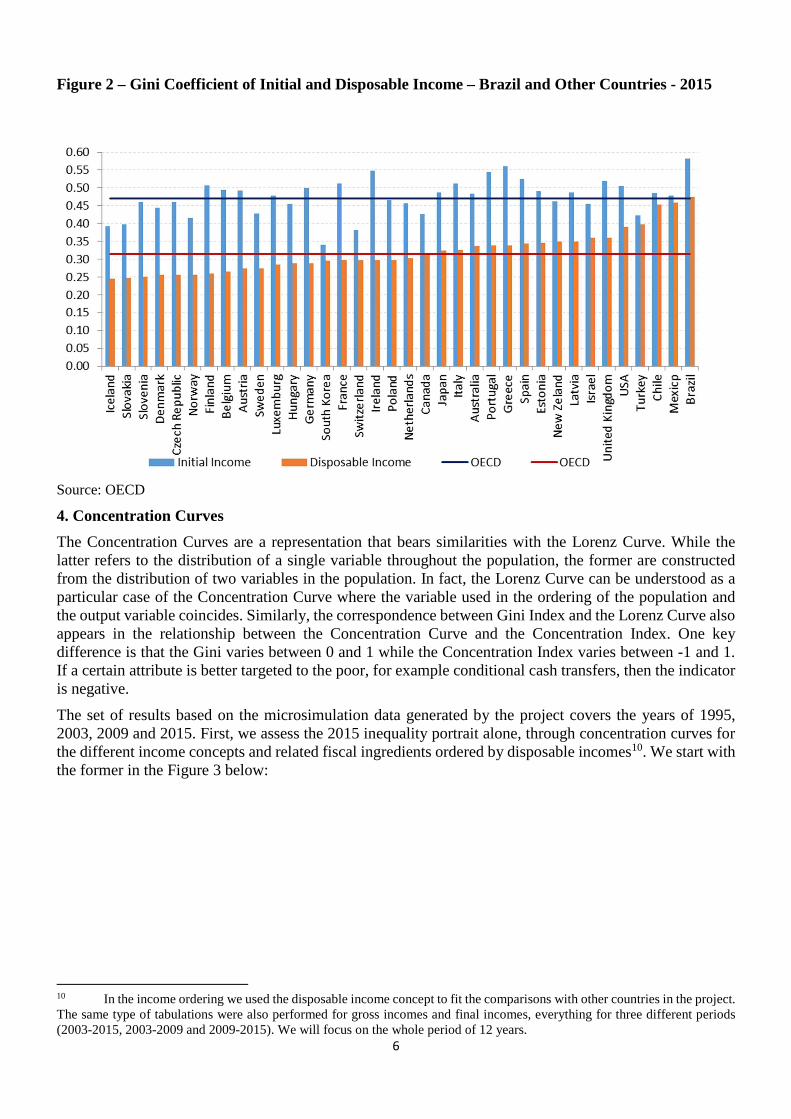
A useful exercise in the investigation of the impact of a tax-benefit system on inequality is to perform a comparative analysis of the country in question relatively to the international experience. The Figure 2 below illustrates such an analysis by comparing Brazil’s Gini coefficient for initial and disposable income with the respective Gini coefficient for a sample of other countries and with the OECD average.

9 The Gini coefficient is a standard measure of inequality, which varies from 0 to 1. The closer to 1 the coefficient the higher the level of inequality.

6

Figure 2 – Gini Coefficient of Initial and Disposable Income – Brazil and Other Countries - 2015

Source: OECD

4. Concentration Curves

The Concentration Curves are a representation that bears similarities with the Lorenz Curve. While the latter refers to the distribution of a single variable throughout the population, the former are constructed from the distribution of two variables in the population. In fact, the Lorenz Curve can be understood as a particular case of the Concentration Curve where the variable used in the ordering of the population and the output variable coincides. Similarly, the correspondence between Gini Index and the Lorenz Curve also appears in the relationship between the Concentration Curve and the Concentration Index. One key difference is that the Gini varies between 0 and 1 while the Concentration Index varies between -1 and 1. If a certain attribute is better targeted to the poor, for example conditional cash transfers, then the indicator is negative.

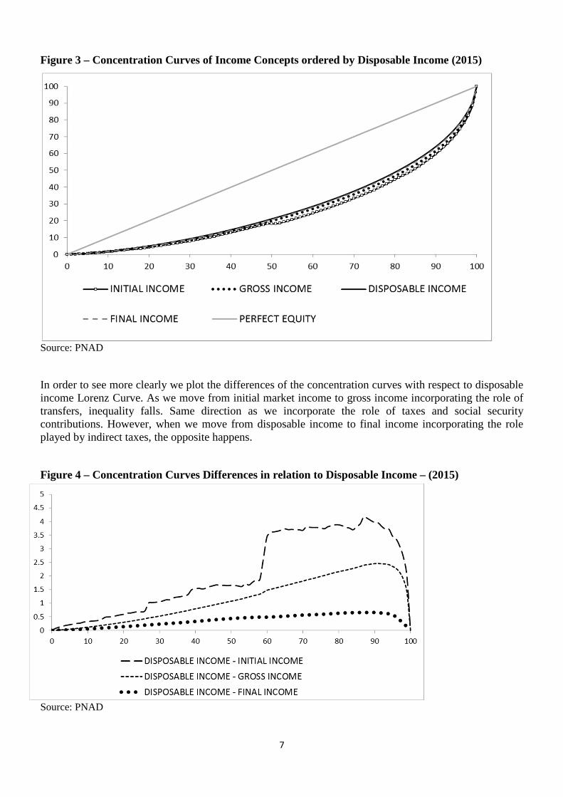
The set of results based on the microsimulation data generated by the project covers the years of 1995, 2003, 2009 and 2015. First, we assess the 2015 inequality portrait alone, through concentration curves for the different income concepts and related fiscal ingredients ordered by disposable incomes10. We start with the former in the Figure 3 below:

10 In the income ordering we used the disposable income concept to fit the comparisons with other countries in the project. The same type of tabulations were also performed for gross incomes and final incomes, everything for three different periods (2003-2015, 2003-2009 and 2009-2015). We will focus on the whole period of 12 years.

7

Figure 3 – Concentration Curves of Income Concepts ordered by Disposable Income (2015)

Source: PNAD

In order to see more clearly we plot the differences of the concentration curves with respect to disposable income Lorenz Curve. As we move from initial market income to gross income incorporating the role of transfers, inequality falls. Same direction as we incorporate the role of taxes and social security contributions. However, when we move from disposable income to final income incorporating the role played by indirect taxes, the opposite happens.

Figure 4 – Concentration Curves Differences in relation to Disposable Income – (2015)

Source: PNAD

8

We present in the next Figure 5 the concentration curves for different official cash transfers. Graphically, the most well targeted indicators for 2015 are Family Grant (PBF) and Poor Elderly/Disability benefits, followed by subsidies to formal employment and unemployment benefits. Public pensions’ curves show higher inequality and given its size are close to total cash transfers11. Both curves are closer to disposable income curve than targeted cash transfers are.

Figure 5 – Concentration Curves of Cash Transfers ordered by Disposable Income (2015)

Source: PNAD

Finally, we analyse the curves for different taxes and contributions. Since it has a negative sign in the budget constraint, the closer to the perfect equality line the more regressive is the expense. The most unequal are indirect taxes followed by social security contributions and personal income taxes.

11 Although, these curves are expressed in per capita terms some of them present mass concentration in similar points

as expressed in individual incomes curves.

9

Figure 6 – Concentration Curves of Income Concepts ordered by Disposable Income (2015)

Source: PNAD

Figure 7 below presents the evolution of the concentration curve of the Family Grant programme (PBF) in 2003, 2009 and 2015. As the programme expanded it became somewhat less targeted12 but as we have seen previously it still more inclusive than other social programmes in the final 2015 year.

Figure 7 – Concentration Curves for the Family Grant Programme ordered by Disposable Income

Source: PNAD

12There is not inequality dominance between years since the concentration curves cross.

10

The concentration curve allows to evaluate how progressive are different fiscal ingredients in isolation. However, we will build an integrated framework of the static and dynamic impacts of these components. The following section presents a framework to measure the social impacts of taxes and transfers that will be applied to Brazilian data. One advantage of this approach is to address these dimensions both in levels and in growth rates.

5. How Progressive are Incomes, Transfers and Taxes? A Framework

5.1 Portrait

We depart from Tony Atkinson seminal contribution of decomposing social welfare into mean and inequality components applied by Amartya Sen to the case of the Gini the most popular inequality index.

=−= )1( GW µ �� (1)

Where G is the Gini index, which is a relative measure of inequality. E=(1-G) is a measure of equity in income.

Taking logarithm of both sides of (1) gives

����� = ����� + ����� (2)

Which on taking the first difference gives

�∗ = � + (3)

where �∗ = ∆����� is the growth rate of social welfare W, � = ∆����� is the growth rate of average income of the society and = ∆����� is the social welfare growth rate, which will be positive (negative) if growth is pro-poor (anti-poor).

Taxes and Transfers

Suppose households draw their income from k sources with total per capita income x such that

� = ∑ ������ (4)

This equation can be used to estimate the contributions of each income source (component) to average income of the population. 100 × ��/� is the percent contribution of the ith income source or taxes to the total average income.

Similarly, we can calculate the mean social welfare of the ith income source from (4) as:

� = ∑ ������ (5)

This equation provides the contribution of each income component to total social welfare. 100 ��/� is the percent contribution of the ith income source to total social welfare.

The mean social welfare of the ith income component in (5) can also be written as

�� = ���1 − ��� = ���� (6)

where Ci is the concentration index of the ith income component.

11

The concentration index Ci informs how the ith income component is distributed across income ranges. The concentration index lies between -1 and +1. Suppose the ith income component is the income received by beneficiaries of the Bolsa Família Programme (BFP), then for instance if the concentration index is 0, then all individuals in the society are equal beneficiaries, if Ci =-1, then the poorest person receives all the benefits of the programme and if Ci =+1, then the richest person receives all benefits. The concentration index is a measure of inequity of an income component. Therefore, a measure of equity of the ith income component is defined as �� = �1 − ���, so the larger the value of Ei the more equitable will be the ith income component. Ei equals 1 if all individuals enjoy the same ith component income. This could be the benchmark: as such, the ith component is equitably (inequitably) distributed if Ei is greater (less) than 1.

Substituting (4) and (6) into (5) gives

� = ∑ �����

���� (7)

which shows that equity in total income is a weighted average of equity in each income component where weights are proportional to the shares of income components in the mean income.

Taking logarithms and first differences of both sides of (6) gives

∆������ = ∆������ + ∆������ (8)

Denoting

��∗ = ∆������

�� = ∆������

� = ∆������

which gives

��∗ = �� + � (9)

which shows that growth rate of social welfare for the ith component is a sum of the two growth rates: (1) growth rate of mean of the ith income component and (2) growth of equity index of the income component. We define the growth of the ith income component as pro-poor (anti-poor) if the equity index of the ith income component increases (decreases). Thus, the i th component is pro-poor (anti-poor) if there is a gain (loss) in growth rate of welfare of the ith income component.

5.2 Fiscal Determinants of Social Welfare Growth

This section presents a methodology to calculate the contribution of various income sources to the total pro-poor growth rate. For instance, it will inform how much different social welfare programmes contribute to the total pro-poor growth of income13.

Suppose �� is the mean of per capita income in year t and ��� is the mean of the ith income component in year t. Then based on (4) we have

�� = ∑ ������� (10)

It can be shown that

∆������~�

�∑ �����

���� !���� !�

+ ������∆������� (11)

13 Kakwani et al. (2010) develop a dynamic analysis framework using another social welfare function.

12

which shows that the growth rate of per capita mean income is the weighted average of the growth rates of individual income components - the weights being proportional to the average of income shares in each period. This equation informs the magnitude of the contribution of each income component to the growth rate of per capita mean (average standard of living).

Suppose Wt is the social welfare in year t and Wit is the social welfare of the ith income component, then based on (10) we have

�� = ∑ ������� (12)

Then it can be shown that

∆������~�

�∑ �����

"��� !�

"�� !�+ "��

"��∆������� (13)

which shows which shows that the growth rate of social welfare is the weighted average of the growth rates of social welfare of individual income components – the weights being proportional to the average of social welfare shares in each period. This equation informs the magnitude of contribution of each income component to the growth rate of social welfare.

The pro-poor growth rate from (3) is given by

� = ∆������ − ∆������ (14)

Which in view of (16) and (18) gives the contribution of each income component to the pro-poor growth rate of per capita total income.

5.3 Targeting Indicator

The small contribution of Bolsa Família to inequality reduction does not imply that the programme is not well targeted to the lower income families. Policy making will benefit from determining the targeting efficiency of various income sources, which income sources contribute more to social welfare and by how much. An income source can be said well targeted to low income families if it contributes more to social welfare relative to its contribution to income. This motivates us to propose a new index:

#� ="��

"��= $�

$ (15)

Where Ei = (1-Ci ) is a measure of equity of the ith income component and E = (1-G) is a measure of equity of total income.

If #� is greater than 1, this implies that controlling for the income share, the ith income source contributes more to social welfare. This index is like a targeting index informing how well a particular income source is targeted to the lower income families. The targeting indicator for total income is 1, which is the benchmark. An index value greater than 1 implies that the particular income source benefits the lower income families more than the average. The larger is the value of index, the greater the targeting efficiency.

This same measure of equation (15) can also be analysed in a dynamic fashion comparing changes in social welfare and changes in the fiscal cost associated with it.

13

6. Measuring the Social Welfare Impacts of Taxes and Transfers over time (2003 to 2015)

6.1 Social Welfare Static Decompositions

As the methodology developed in section 5, the Table 3 below presents mean income, inequality14 and social welfare levels associated with different income concepts and respective fiscal ingredients between them ordered by disposable income. This methodology allows us to map the contribution of different taxes and transfers into disposable income based mean, inequality and social welfare.

Table 3 – Mean Income, Inequality and Social Welfare Levels – Disposable Income (2003 to 2015)

Source: PNAD

The following Table 4 organizes selected pieces of information on Table 3 in terms of the Social Welfare Benefit/Fiscal Cost ratio, which corresponds, by construction, to the complement of the Concentration Ratio, a term that provides how much each real of public transfers affected on average the level of social welfare. Implicitly, the analysis evaluate the overall impact of all the resources spent in each monetary transfer programme, leaving aside impacts on the margin and other desired long run impacts of each of these income policies on education, employment or income stability, for example. The results show that Family Grant is the best public policy in terms of social welfare generated by each fiscal cost.

14 A product between the concentration index of the income concept times its share in the mean disposable income.

14

Table 4 – Static Targeting Indicator of Cash Transfers: Social Welfare /Fiscal Cost Levels in 2015 (ordered by Disposable Income)

Source: PNAD

6.2 Social Welfare Dynamic Decompositions

Looking at the statistics revealed in previous Tables 3 and 4, in 2015 the social welfare for disposable income was below the mean due to the discount factor of 47.64% captured directly by the impact of the Gini coefficient. In 2003, this difference was even higher: 55.59% due to higher inequality. One can grasp the same impact using the Table 5 below that looks at growth rates. The annual rate of growth of social welfare (4.86%) was higher than of mean income (3.48%) due to the equalization effect (1.37%).

Table 5 – Income, Equality and Social Welfare –Annual Growth Rates – Disposable Income

Source: PNAD

The Table 5 above shows an impressive rise in the mean income of anti-poverty policies, as the family grant conditional cash transfer programme (18.27%). What is the net effect of an increasing role of this better targeted– but increasingly less so, as we have seen in its concentration curves evolution in time - social programme in overall social welfare?

15

Although, the previous Table is useful, if one is interested into capturing the role of each ingredient, one should also take into account the weights of these ingredients. The main advantage of the decomposition methodology explored here is to allow moving directly from the levels of each component to its contribution to social welfare rates of change. Incorporating not only its growth but also its weight in each income concept, we deconstruct the whole effect into smaller components associated with private incomes, public transfers and taxes. Each of these components of the social welfare impact can be further decomposed into its respective mean and inequality drivers.

Table 6 – Income, Equality and Social Welfare Growth - Contribution by Component – Disposable Income (2003 to 2015)

Source: PNAD

The period between 2003 and 2015 verified a decrease in inequality and an increase in the mean income and the social welfare of the population for all the different income concepts and their components. The data ordered by disposable income disclosed that inequality explained 28.4% while mean income explained the remainder 71.6% of a yearly social welfare growth of 4.86% in that period.

Finally, we focused on the following Table 7 that presents the list of cash transfers policies to measure each relative contribution to social welfare growth in comparison with their relative contribution to income increase during the same period. The results show that Family Grant, the main income policy designed for poverty alleviation in Brazil, is indeed the one better targeted to the poor, since its contribution to the rise of social welfare is 2.7 times the contribution to the rise of mean income.

16

Table 7 - Dynamic Targeting Indicator of Cash Transfers: Social Welfare/Fiscal Cost Growth – Relative Contribution Based on Disposable Income from 2003 to 2015

Source: PNAD

7. Poverty Impacts

Brazil adopted an official extreme poverty line around U$S 1.25 using older Purchasing Power Parity (PPP) which is perhaps too low for Brazilian level of income. We perform different exercises using different international poverty lines, recently raised from the use of the new Purchasing Power Parity (PPP) estimates.

Table 8 – Proportion of Poor (P0) and Poverty Gap (P1) for Disposable Income Concept and Different Poverty Lines - 2003 and 2015 –

Source: PNAD

The first poverty related contribution of this work is to analyse the impacts of inequality on poverty changes using our microsimulation framework of fiscal instances. The fall of poverty in percentage points increases with the level of the poverty line used, which is not surprising because poverty levels are also necessarily higher. However, the proportional variation is monotonically higher for higher poverty aversion coefficients (i.e. P1 over P0) and for lower poverty lines ranging from -95.91% to -65.92% in the case of the poverty gap (P1). Using as a benchmark the intermediary U$S 3.2 dollars a day line the fall in the 2003 to 2015 period amounted to -18.8 percentage points or a reduction of 69 %. This means that poverty fell nearly twice more than expected in the UN first MDG in less than half of the period.

We apply standard Ravallion-Datt decomposition into growth and inequality components to assess their relative roles using initially the concept of disposable income. The most important dimension analysed here is the relative share of poverty fall explained by inequality that falls monotonically in the case of P1as the

17

poverty line rises ranging from 65.44% to 40% of total poverty fall. In the case of our intermediary U$S 3.2 dollars a day line 43 % of total P1 fall was explained by the inequality component. Almost a middle path driven by both distributive and growth dimensions.

Table 9 – Poverty Variation between 2003 and 2015 for Disposable Income Concept

Source: PNAD

Anti-Poverty Programmes Efficiency

We also developed an index to assess pro-poor policies as the ratio between the social gains obtained with a specific programme impact on poverty over its fiscal cost ordered by a particular income concept in a specific moment in time. We define the social gains as the negative variation of poverty in percentage points due to the programme impacts, while its fiscal cost as the programme’s participation in the mean income. Thus, the equation (16) would be written as follows:

%&� = −∆'(��)��

= −*'(�+',(�-

�)�� (16)

Where ∆.�� is the difference between the actual poverty level (.) in comparison with a hypothetic scenario of poverty (./) where a specific programme p were not implemented and �&�� is the mean income of this programme. Either �&,., ./ are defined in relation to a specific income component, for example, disposable income. Consequently, the mean income of the programme p can also be interpreted as the difference in the mean income of the specific income concept due to the existence of this programme. Therefore, %� can be interpreted as the ratio between the relative participation of the programme p in poverty and its relative participation in the mean income. The negative symbol in equation (16) also implies that the larger is the value of the index, the greater the targeting efficiency.

The next exercise is to simulate statically for 2015 the benefit in terms of poverty fall associated with each government cost of different anti-poverty. We compare Family Grant (BFP) and Poor Elderly/Disability benefits (BPC) impacts by comparing the scenarios of poverty with and without these programmes.

18

Table 10 – Poverty Scenarios If Main Poverty Alleviation Policies did not exist – 2015

Source: PNAD

The key statistic is the net benefit in terms of poverty fall per monetary unit spend as in Table 11 below. Except for the highest poverty line, the social benefit is higher for Family Grant for all poverty lines and poverty measures considered. In our benchmark (P1 with the intermediary line), this ratio is 119.73% higher for the Family Grant Programme (Campelo and Neri 2013; Peci and Neri 2017).

Table 11 – Poverty Comparison: Reality versus Scenarios If Main Poverty Alleviation Policies did not exist – 2015

Source: PNAD

8. Conclusion

This paper assesses fiscal redistribution in Brazil between 2003 and 2015. The framework proposed evaluate in an integrated manner causes and consequences of inequality in terms of social welfare and poverty both in levels and changes over time.

The paper develops, describes and applies an empirical methodology, including the source of micro data used, Brazilian institutional features, data adjustments made, simulation procedures adopted and the results thereupon generated. This paper had the initial objective of providing a report on the procedures adopted in the ongoing work concerning the fiscal redistributive impact of the Brazilian tax-benefit system. This work necessarily involves methodological decisions made in order to be able to model the system as close

19

as possible to its actual operation. It is thus important to have it clear in mind what are the steps followed to generate the information used in the analysis.

The general approach here delineated is applied to each of the four years to be covered in this study (1995, 2003, 2009, and 2015) to allow a compatible comparative analysis for the period considered. We compare different income concepts but focus here on derived per capita disposable income changes between 2003 and 2015. Other contribution of this paper is to simulate a concept that is not readily available in Brazilian household surveys. Around 28.2% of per capita disposable Gini index based social welfare measure changes is due to pure inequality fall while the remainder is due to mean growth. Our results also suggest that official cash transfers accelerated the growth of social welfare while direct and indirect taxes changes played the opposite role. The analysis of the role played by specific fiscal instruments among various taxes and cash transfers programmes shows that Family Grant programme was the better targeted action in the 2003 to 2015 period using both social welfare and poverty criteria.

References

Alvaredo, F. 2011. A note on the relationship between top income shares and the Gini coefficient. Economic Letters, Vol. 110, 274-277.

Atkinson, A.B. 2007. Top Incomes Over the Twentieth Century: A Contrast Between European and English Speaking Countries. Oxford: Oxford University Press.

Barreix, A., J. C. Benítez and M.Pecho. 2017. Revisiting personal income tax in Latin America: Evolution and impact. OECD Development Centre, WorkingPaper No. 338.

Campello, T. Neri, M. C.; (Org.) . Programa Bolsa Família: uma década de inclusão e cidadania. 1. ed. Brasília: IPEA, 2013. v. 1. 494p .

Higgins, S. and C. Pereira. 2013. The effects of Brazil’s high taxation and social spending on the distribution of household spending. CEQ Working Paper No. 7, Tulane University.

Immervoll, H., H. Levy, J. R. B. Nogueira, C. O’Donoghue, and R. B. Siqueira. 2009. The impact of Brazil’s tax-benefit system on inequality and poverty, in S. Klasen and Nowak-Lehmann (eds.), Poverty, Inequality, and Policy in Latin America. Cambridge: MIT Press.

Kakwani, N. ; Neri, M. C.; Son, H. . Linkages Between Pro-Poor Growth, Social Programs and Labor Market: The Recent Brazilian Experience. World Development, v. 38, p. 881-894, 2010.

Medeiros, M., P. H. Souza and F. A. Castro. 2015. O topo da distribuição de renda no Brasil: primeiras estimativas com dados tributários e comparação com pesquisas domiciliares, 2006-2012. Revista de Ciências Sociais, Vol. 58, No. 1.

Peci, A; Neri, M. C.. Revista Brasileira de Administração Pública - Special Issue on Public Policies on Fighting Poverty. 00. ed. Rio de Janeiro/RJ: , 2017. v. 01. 00p .

Seae/MF. Efeito Redistributivo da Política Fiscal no Brasil. 2017. Brasília, Secretaria de Acompanhamento Econômico, Ministério da Fazenda.

Secretaria da Receita Federal. 2017. Grandes Número IRPF – Ano Calendário 2015, Exercício 2016. Brasília.

Silveira, F. G., F. Rezende, J. R. Afonso and J. Ferreira. 2013. Fiscal equity: distributional impacts of taxation and social spending in Brazil. Working Paper 115, International Policy Centre for Inclusive Growth, Brasília.