Chapter 8 Fiscal Uncertainty:The Enemy of Efficient Budgeting This chapter analyzes, or in some cases updates and reanalyzes, the impact of Ascal institutions on state Ascal policy. The conclusions about certain Ascal institutions generally conform to those in prior studies. However, conducting the empirical analysis with a uniform set of control variables and within a common time period facilitates a comparison of the relative impact of various institutions. 1 The chapter breaks new ground in several respects. Like prior studies, the models examine the impact of institutions on the size of government, looking at spending, revenues, and taxes. Beyond that, the analysis examines both theoretically and empirically the relation- ship between Ascal volatility and state spending. Fiscal volatility cre- ates uncertainty with respect to future operations of government agencies, and this impedes the selection of efAcient production processes. This extension of the mean-variance perspective to state Ascal performance adds another dimension to the study of Ascal in- stitutions. The models proceed to examine the impact of institutions on the volatility of state budgets and through this channel their indi- rect effects on the size of government. Fiscal Volatility and the Size of Government The analysis seeks to explore a new dimension in Ascal policy: the re- lationship between the predictability of government budgets and their size. 2 Elementary economic theory teaches us that, to minimize production costs, factors such as land, labor, and capital will be em- ployed in accord with their marginal productivities relative to their marginal costs. The particular input mix that yields the greatest ef- Aciency depends in part on the available technology, on the speed with which factors employed in production may be adjusted, and on how much output Bexibility is required. Technology-related con- straints are typically handled by the analytical distinction between short-run and long-run adjustment paths. Given a sufAcient time to 96
Transcript
Chapter 8
Fiscal Uncertainty:The Enemy of Efficient Budgeting
This chapter analyzes, or in some cases updates and reanalyzes, theimpact of Ascal institutions on state Ascal policy. The conclusionsabout certain Ascal institutions generally conform to those in priorstudies. However, conducting the empirical analysis with a uniformset of control variables and within a common time period facilitatesa comparison of the relative impact of various institutions.1
The chapter breaks new ground in several respects. Like priorstudies, the models examine the impact of institutions on the size ofgovernment, looking at spending, revenues, and taxes. Beyond that,the analysis examines both theoretically and empirically the relation-ship between Ascal volatility and state spending. Fiscal volatility cre-ates uncertainty with respect to future operations of governmentagencies, and this impedes the selection of efAcient productionprocesses. This extension of the mean-variance perspective to stateAscal performance adds another dimension to the study of Ascal in-stitutions. The models proceed to examine the impact of institutionson the volatility of state budgets and through this channel their indi-rect effects on the size of government.
Fiscal Volatility and the Size of Government
The analysis seeks to explore a new dimension in Ascal policy: the re-lationship between the predictability of government budgets andtheir size.2 Elementary economic theory teaches us that, to minimizeproduction costs, factors such as land, labor, and capital will be em-ployed in accord with their marginal productivities relative to theirmarginal costs. The particular input mix that yields the greatest ef-Aciency depends in part on the available technology, on the speedwith which factors employed in production may be adjusted, and onhow much output Bexibility is required. Technology-related con-straints are typically handled by the analytical distinction betweenshort-run and long-run adjustment paths. Given a sufAcient time to
96
adjust all factors, capital investments will be made to adopt the cost-minimizing technology to produce any level of output. The degree ofBexibility required typically depends on how widely demand Buctu-ates over time. These two temporal elements may clash, and this addsa crucial element into the choice of an optimal production process.
The trade-off between output volatility and efAciency is describedwith reference to Agure 8.1. Consider a government agency planningits future operations for the next two Ascal years, FY1 and FY2. By as-sumption this agency seeks to minimize operating costs, including allcapital costs. The agency must select one of two alternative produc-tion processes, the �-process or the �-process. Figure 8.1 shows thetotal cost functions associated with these two processes, labeled TC�
and TC�, assumed for simplicity to be linear. These total cost rela-tionships characterize the agency’s operations in each Ascal year. The�-process requires a larger locked-in investment than the �-process,and by assumption this investment is irreversible over the two-yearplanning horizon. These different capital requirements mean that themarginal costs under the �-process exceed marginal costs under the�-process, which is reBected by the relative slopes of the two totalcost functions. For example, the �-process can accommodate outputreversals more efAciently than the �-process because it embracesshort-term leases rather than constructing new facilities or it per-forms functions in-house rather than committing to long-term out-sourcing contracts.
Under the budget process posited here, the agency knows its ex-pected output in the initial Ascal period, labeled Q1 in Agure 8.1. Byconstruction, the cost of producing Q1 is the same, $600 million, usingeither the �-process or the �-process. The agency’s decision to adoptthe �-process or the �-process thus depends on its expected output inFY2. Let QL and QH stand for two possible outcomes in FY2, the ArstreBecting a lower output and the second reBecting a higher outputrelative to Q1. If high output level QH were known with certainty, the�-process would be more efAcient than the �-process and thereforeselected. If the low output level QL were known with certainty, the �-process would be selected.
In contrast to these two certain outcomes, suppose the agency asan integral part of its planning exercise must predict the probabilityof QL or QH. To make the analysis as simple as possible, suppose QLand QH are equally probable, or Prob (QL) � 0.5 and Prob (QH) �0.5. This means of course that the agency can do no better than tochoose a process randomly and that the wrong process (that is, the
Fiscal Uncertainty 97
process that would not yield the lowest cost) will be selected half ofthe time. Under this uncertain Ascal environment, the agency’s ex-pected costs would be $100 million higher than they would be undera certain Ascal environment. That is, with probability 0.5 the agency’srandom choice proves correct, either selecting the �-process and QLmaterializes or selecting the �-process and QH materializes. Withprobability 0.5 the agency’s choice proves incorrect, and given an in-correct choice, costs exceed the minimum cost level by $200 million.3
As this simple model illustrates, uncertainty about future outputrates conveys risks associated with long-run operations relative to amore predictable Ascal environment.The empirical models presentedlater in the chapter explore whether and to what extent the postu-lated trade-off between volatility and efAciency systematically affectsgovernment spending levels.
98 Volatile States
$ (Millions)
TCα
900
700 TCβ
600
500
300
QL Q1 QH
Agency Output per Fiscal Year
Fig. 8.1. Uncertainty of future funding levels and agency costs
Mechanisms for Fiscal Discipline:Which Fiscal Rules Work?
Shaped by a century of presidential appeals for an item veto of ap-propriations measures and of pleas for a balanced budget amendmentto the Constitution, much of the debate about budget process reformat the U.S. federal level has concentrated on these two institutions.4
Naturally, the differences among states with respect to these two in-stitutions invite empirical scrutiny. These and three other institutionsthat have been identiAed in prior research as potentially importantare brieBy described, and the next section examines the impact ofthese institutions on state Ascal outcomes. As previewed in the intro-duction to this chapter, the empirical section investigates the direct ef-fects on spending levels (the standard approach in the literature) andthe indirect effects on Ascal volatility.
Balanced Budget Rules
Every state except Vermont has a balanced budget requirement.However, the details of these 49 state requirements differ in an im-portant respect, namely, the stage in the budget process at which bal-ance is required. A survey of past research points to four categoriesof requirements. The weakest standard requires the governor to sub-mit a balanced budget. A stricter standard requires the legislature topass a balanced budget. Under these two categories actual expendi-tures may exceed revenues if end-of-year realizations happen to di-verge from the enacted budget. The third standard requires the stateto acknowledge its deAcit but allows the deAcit to be carried over intothe next budget with no consequences. Bohn and Inman (1996) aptlylabel these three categories “prospective budget constraints.” Thefourth and strictest form of balanced budget rule combines the prac-tice of enacting a balanced budget with a prohibition on a deAcit carry-forward. Bohn and Inman label this strictest form a “retrospectivebudget constraint.”While numerous studies have examined state bal-anced budget rules, three studies convincingly advance the idea thatthe retrospective standard has a signiAcant impact on Ascal policy,whereas the other three do not.
Bohn and Inman And that balanced budget rules that prohibit thecarryover of end-of-year budget deAcits have a statistically signiAcanteffect, reducing state general fund deAcits by $100 per person. In con-trast, soft or prospective budget constraints on proposed budgets donot affect deAcits. Moreover, the deAcit reduction in retrospective
Fiscal Uncertainty 99
budget constraint states comes through lower levels of spending andnot through higher tax revenues.
Poterba (1994) examines the Ascal responses in states to unex-pected deAcits or surpluses. He compares the adjustments to Ascalshocks under “weak” versus “strict” antideAcit rules, categories thatclosely resemble the Bohn-Inman division. Poterba’s results suggestthat states with weak antideAcit rules adjust less to shocks than stateswith strict rules. A $100 deAcit per person overrun leads to only a $17per person expenditure cut in a state with a weak rule and to a $44cut in states with strict rules. Poterba also Ands no evidence that anti-deAcit rules affect the magnitude of tax changes in the aftermath ofan unexpected deAcit.
Alt and Lowry (1994) focus on the role of political partisanship inAscal policy. They examine reactions to disparities between revenuesand expenditures that can exist even in states with balanced budgetrequirements. In states that prohibit deAcit carryovers, the party incontrol matters. In Republican-controlled states, they And that a onedollar state deAcit triggers a 77¢ response through tax increases orspending reductions. In Democrat-controlled states a one dollardeAcit triggers a 34¢ reaction. In states that do not prohibit carry-overs, the adjustments are 31¢ (Republicans) and 40¢ (Democrats).This evidence suggests that state politics plays an important role andthat antideAcit rules affect Ascal actions.
Following these important studies, the empirical analysis focuseson the effects of strict balanced budget requirements, those that pro-hibit deAcit carryovers from one Ascal year to the next.
The Item Reduction Veto
Governors in all but Ave states have the ability to veto a particularitem in an appropriations bill, in addition to their normal authority toveto an entire bill. Several studies on the Ascal impact of the itemveto provide mixed and inconclusive results. Bohn and Inman (1996)And that the item veto generally has no statistically signiAcant rela-tionship to state general fund surpluses or deAcits. Carter and Schap(1990) And no systematic effect of the item veto on state spending.Holtz-Eakin (1988) Ands that when government power is divided be-tween the two parties, one controlling the executive branch and theother controlling the legislative branch, the item veto helps the gov-ernor reduce spending and raise taxes. Holtz-Eakin Ands that, underpolitical conditions of nondivided government, the item veto yieldslittle, if any, effect.
100 Volatile States
The Holtz-Eakin study stressed that the item veto powers differamong states, and Crain and Miller (1990) examine these differentpowers in further detail. They And that, in contrast to a generic clas-siAcation of the item veto, a particular form of the item veto—the so-called item reduction veto—signiAcantly reduces spending growth.Of the 45 states that have an item veto, 10 give their governors theauthority to either write in a lower spending level or veto the entireitem.The Crain and Miller article argues that the item reduction vetodiffers from the standard item veto because it provides the governorwith superior agenda-setting authority. For example, a governorfaced with excessive funding for a remedial reading program is un-likely to veto the measure but likely would consider a marginal re-duction in the amount of funding for that type of program. Based onthis Anding, the analysis examines in new detail the Ascal impact ofthe item reduction veto.
Tax and Expenditure Limitations
The earliest studies of tax and expenditure limitations (TELs) con-cluded that they have virtually no effect on state Ascal policy (e.g.,Abrams and Dougan 1986). Elder (1992) was among the Arst studiesto examine TELs using an empirical model that controlled for otherfactors (such as income and population) that inBuence spending.With this improved speciAcation Elder Ands evidence that TELs re-duce the growth of state government.
Eichengreen (1992) estimates regression models for both thelevel and the growth rate in state spending as a function of the pres-ence of tax and expenditure limits and the interaction between theselimits and the state’s personal income growth rate. He Ands that theinteraction term is particularly important because limits are typicallyspeciAed as a fraction of personal income. In states with slow incomegrowth rates, limitation laws have had a more restrictive effect ongovernment growth than in states with fast income growth rates.Shadbegian (1996) speciAes an almost identical empirical model,again taking into consideration the interaction between state incomeand TELs.
Reuben (1995) develops an empirical speciAcation that controlsfor the potential endogeneity problem that the passage of tax limitsmay be related to a state’s Ascal conditions. Reuben Ands that whenthese institutions are treated as endogenous the explanatory powerof the institutional variables rises markedly; the estimated effects in-dicate that TELs signiAcantly reduce state spending.
Fiscal Uncertainty 101
Supermajority Voting Requirement for Tax Increases
Knight (2000) points out that, in addition to the 12 states that haveenacted supermajority requirements, 16 states have introduced pro-posals to enact such requirements. Adding a supermajority voting re-quirement to the U.S. federal budget process is also a popular reformmeasure. Two empirical studies have analyzed the effect of superma-jority requirements on state Ascal outcomes. Crain and Miller (1990)And that such rules reduce the growth in state spending by about 2percent based on a relatively short sample period, 1980–86.The studyby Knight (2000) expands the sample period; employs pooled time-series, cross-sectional data; and uses state and year Axed-effects vari-ables. He Ands that supermajority requirements decrease the level oftaxes by about 8 percent relative to the mean level of state taxes.
Budget Cycles
Since 1977 a number of proposals have been introduced in the U.S.House and Senate to lengthen the federal budget cycle from an an-nual to a biennial process. The perception behind these proposals isthat a federal biennial budget would help curtail the growth of fed-eral expenditures. Motivated by these federal proposals, the U.S.General Accounting OfAce (1987) conducted a study of the state ex-periences. That study reports a positive correlation between statespending and annual budget cycles.5
Kearns (1994) lays out the theoretical issues and provides the mostcomprehensive empirical study of state budget cycles to date. Kearnspresents two competing hypotheses. On the one hand, a biennial bud-get transfers power over Ascal decisions from the legislative branchto the governor. This power transfer reduces spending activities asso-ciated with logrolling and pork barrel politics because legislatorsfavor programs that beneAt their narrow, geographically based con-stituencies. The main costs of such geographically targeted programsmay be exported to nonconstituents. By comparison, the governormakes Ascal decisions based on more inclusive beneAt-cost calcula-tions because he or she represents a broader, statewide constituency.In other words, at-large representation mitigates the Ascal commonsproblem. Offering an alternative hypothesis, Kearns posits that a bi-ennial budget cycle imparts durability to spending decisions andthereby encourages political pressure groups to seek governmentprograms.6 Kearns concludes in favor of the latter thesis based on her
102 Volatile States
Anding that states with biennial budgets have higher spending percapita than states with annual budgets.
A third and original hypothesis derives from the conceptualframework developed in the prior section. Namely, lengthening thebudget cycle adds predictability to agency funding levels, facilitatingthe development and execution of efAcient operating plans.
Model Specification Issues and Empirical Results
The empirical model to investigate the impact of Ascal volatility andAscal institutions is developed in three steps beginning with equa-tion (8.1).
Expenditureit � ��it � �i � �t � εit. (8.1)
The estimates use two forms of the dependent variable, Expenditureit:one divides state spending by state personal income, and the other di-vides state spending by state population. The expenditure per capitavariable and all dollar-denominated variables used in the models areadjusted for inBation using 2000 prices as the base year. The datasample pools time-series and cross-sectional data, the variable sub-script i denotes an observation on an individual state, and the subscriptt denotes an observation in a particular year. �i represents a set of statedummy variables, one for each state in the sample, and �t represents aset of time dummy variables, one for each year in the sample.
In equation (8.1) �it represents a vector of variables that control foreconomic and demographic factors that inBuence state governmentspending. These variables include income per capita, the unemploy-ment rate, population, the percentage of the population residing inurban areas, and the percentage of the population between the ages of18 and 64. This set of control variables fairly represents the variablesin prior studies on state spending, and the underlying rationale re-quires only brief explanation.7 Income per capita proxies both the de-mand for public sector services as well as the size of the potential taxbase. The unemployment rate proxies potential claims for unemploy-ment insurance and related welfare programs. Population controls foreconomies of scale in publicly provided services, and per capita costspredictably fall as population increases. Similarly, per capita costsshould fall in states with largely urban, relatively concentrated popu-lations.The variable for the percentage of the population between theages of 18 and 64 is included because young residents (less than 18years old) and elderly residents (more than 64 years old) generate the
Fiscal Uncertainty 103
greatest demands for public education, health care, and other socialservices. Thus this variable should vary inversely with governmentspending.
Of course, other factors such as climatic conditions or foreign im-migration may cause spending to differ among the states.The �i (Axed-effects) dummy variables will control for such state-speciAc factors tothe extent that they remain roughly constant over the sample period.Finally, the �t (year-effects) dummy variables control for inBuences onstate spending such as a national recession, changes in federal grantprograms, or changes in the federal tax code.
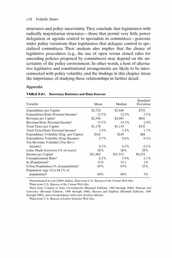
The sample for estimating equation (8.1) includes 47 states(Alaska, Hawaii, and Wyoming are excluded) for the years 1970through 1998. Table 8.A1 in the appendix at the end of this chapterprovides summary statistics for the variables and data sources.
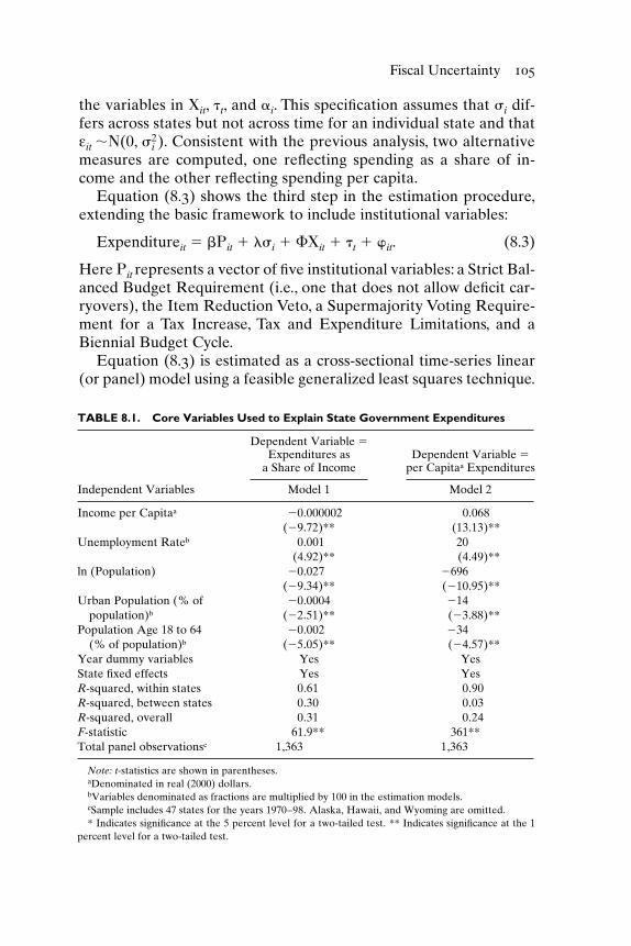
Table 8.1 shows the results of estimating equation (8.1) using thetwo measures of state expenditures: expenditures as a share of in-come (Model 1) and expenditures per capita (Model 2). All the pa-rameter estimates show the expected signs, and the models are esti-mated with a high degree of precision, as indicated by the highadjusted R-squared values and signiAcant F-statistics.The Income perCapita variable has a positive correlation with Expenditures perCapita but a negative correlation with Expenditures as a Share of In-come. This reBects the fact that state spending generally rises or fallswith state income, but less than proportionately. State spendingvaries positively with the unemployment rate. Large states and stateswith largely urban populations experience lower spending (per capitaand as a share of income) than other states, consistent with the econ-omies of scale thesis. Spending declines with the share of a state’spopulation between the ages of 18 and 64, or, to restate this relation-ship more intuitively, spending rises as the share of the populationthat is young or old grows. Finally, all of the �t coefAcients for the yeardummy variables (not reported in the table) are signiAcant.
The analysis next augments this basic model to include the mainvariables of interest, beginning with expenditure volatility. This ex-tension is shown in equation (8.2):
Expenditureit � �i � ��it � �t � it. (8.2)
The additional variable denoted i measures the volatility in statespending. i is the standard deviation of εit, the residuals from themodels estimated using equation (8.1). That is, these residuals repre-sent the deviations in spending from the values predicted based on
104 Volatile States
the variables in �it, �t, and �i. This speciAcation assumes that i dif-fers across states but not across time for an individual state and thatεit ��(0, 2
i ). Consistent with the previous analysis, two alternativemeasures are computed, one reBecting spending as a share of in-come and the other reBecting spending per capita.
Equation (8.3) shows the third step in the estimation procedure,extending the basic framework to include institutional variables:
Expenditureit � � it � �i � ��it � �t � it. (8.3)
Here it represents a vector of Ave institutional variables: a Strict Bal-anced Budget Requirement (i.e., one that does not allow deAcit car-ryovers), the Item Reduction Veto, a Supermajority Voting Require-ment for a Tax Increase, Tax and Expenditure Limitations, and aBiennial Budget Cycle.
Equation (8.3) is estimated as a cross-sectional time-series linear(or panel) model using a feasible generalized least squares technique.
Fiscal Uncertainty 105
TABLE 8.1. Core Variables Used to Explain State Government Expenditures
Dependent Variable �Expenditures as Dependent Variable �
a Share of Income per Capitaa Expenditures
Independent Variables Model 1 Model 2
Income per Capitaa �0.000002 0.068(�9.72)** (13.13)**
Unemployment Rateb 0.001 20(4.92)** (4.49)**
ln (Population) �0.027 �696(�9.34)** (�10.95)**
Urban Population (% of �0.0004 �14population)b (�2.51)** (�3.88)**
Population Age 18 to 64 �0.002 �34(% of population)b (�5.05)** (�4.57)**
Year dummy variables Yes YesState fixed effects Yes YesR-squared, within states 0.61 0.90R-squared, between states 0.30 0.03R-squared, overall 0.31 0.24F-statistic 61.9** 361**Total panel observationsc 1,363 1,363
Note: t-statistics are shown in parentheses.aDenominated in real (2000) dollars.bVariables denominated as fractions are multiplied by 100 in the estimation models.cSample includes 47 states for the years 1970–98. Alaska, Hawaii, and Wyoming are omitted.* Indicates significance at the 5 percent level for a two-tailed test. ** Indicates significance at the 1
percent level for a two-tailed test.
The speciAc procedure used iterates the GLS estimation technique toconvergence. The FGLS technique allows estimation in the presenceof autocorrelation within states and cross-sectional heteroskedastic-ity across states. The FGLS estimation procedure estimates and thenadjusts for systematic patterns in the residuals across states.
Results for Fiscal Volatility
The results of estimating equation (8.3) are divided into two tables.Table 8.2 reports the models that use Expenditures per Capita as thedependent variable. In these models the Expenditure Volatility vari-able is computed based on the deviations in expenditures per capita.Table 8.3 reports the models that use Expenditures as a Share of In-come as the dependent variable. In these models the ExpenditureVolatility variable is computed based on the deviations in expendi-
106 Volatile States
TABLE 8.2. Effects of Fiscal Institutions on State Government Expendituresper Capita
Year dummy variables Yes Yes YesOther variables included, see table 8.1 Model 2 Model 2 Model 2Wald chi-squared 5364** 7407** 7658**Total panel observationsb 1,363 1,363 1,363
Note: Parameters are estimated using cross-sectional time-series FGLS regressions. z-statistics areshown in parentheses.
aExpenditure Volatility is measured as the standard deviation in the regression residuals from thecore model referenced in table 8.1.
bSample includes 47 states for the years 1970–98. Alaska, Hawaii, and Wyoming are omitted.* Indicates significance at the 5 percent level for a two-tailed test. ** Indicates significance at the 1
percent level for a two-tailed test.
tures as a share of income. The model speciAcations reported in thesetwo tables are otherwise identical.To avoid repetition, the results in ta-bles 8.2 and 8.3 do not report the estimated coefAcients for the vectorof control variables (income, unemployment, population, urbaniza-tion, and population age); the parameter estimates on these variablesappear robust with respect to the various model speciAcations.
A Anal element of the estimation strategy requires clariAcation be-fore proceeding to the results. Because the institutional variables of in-terest may affect Expenditure Volatility as well as the level of Expen-ditures, the parameter estimates based on a single equation model(FGLS) may be biased.To take this potential endogeneity bias into ac-count, the coefAcients in equation (8.3) are also estimated using a two-stage method that endogenizes the Expenditure Volatility measures.
Fiscal Uncertainty 107
TABLE 8.3. Effects of Fiscal Institutions on State Government Expenditures as aShare of Income
Dependent Variable � Expenditures as aShare of State Income
Year dummy variables Yes Yes YesOther variables included, see table 8.1 Model 1 Model 1 Model 1Wald chi-squared 2624** 3317** 3698**Total panel observationsb 1,363 1,363 1,363
Note: Parameters are estimated using cross-sectional time-series FGLS regressions. z-statistics areshown in parentheses.
aExpenditure Volatility is measured as the standard deviation in the regression residuals from thecore model referenced in table 8.1.
bSample includes 47 states for the years 1972–98. Alaska, Hawaii, and Wyoming are omitted.* Indicates significance at the 5 percent level for a two-tailed test. ** Indicates significance at the 1
percent level for a two-tailed test.
The Arst stage obtains the predicted value of Expenditure Volatilitybased on the other right-hand side variables, and the second stage usesthis predicted valued in the estimation.8 Tables 8.2 and 8.3 provideboth the single equation FGLS and the two-stage estimation results forcomparison.
The Arst columns in tables 8.2 and 8.3 present the results for equa-tion (8.2), that is, when only the Expenditure Volatility variable isadded to the core model, speciAed in equation (8.1). The estimatedcoefAcient on Expenditure Volatility is positive and signiAcant at the1 percent level in these two models. Expenditure Volatility is also sig-niAcant at the 1 percent level in the other models shown in tables 8.2and 8.3 that include the additional institutional variables. These re-sults strongly support the conceptual framework laid out earlier inthe chapter. Namely, Ascal uncertainty impairs efAciency and raisesthe cost of government programs.
The size of the impact of Expenditure Volatility on spending canbe illustrated using the per capita results in the third column of re-sults in table 8.2. In that (two-stage) model the estimated coefAcientfor Expenditure Volatility is 5.87.9 Consider a 10 percent increase inExpenditure Volatility from its mean value of $162 (a 10 percent in-crease in volatility equals about $16 per capita). The projected im-pact would be a $95 increase in per capita spending (� 5.87 � $16).Using the mean value of per capita spending (� $2,724 for the 1970–98 period), this represents a 3.5 percent increase in per capita spend-ing (� $95/$2,724). This point estimate evaluated at the mean im-plies an elasticity of per capita spending with respect to spendingvolatility of 0.35. As a second illustration of the magnitude of theuncertainty-efAciency trade-off, suppose Expenditure Volatilityrises by one standard deviation (� $68). The projected impactwould be to increase per capita spending by $400 (� 5.87 � $68), a15 percent increase relative to the spending mean (� $400/$2,724).Figure 8.2 illustrates graphically this estimated trade-off betweenbudget volatility and per capita spending. Figure 8.3 illustrates thetrade-off using the estimated results for spending as a share of in-come (from table 8.3).
Of course, this link between volatility and spending can beframed in a constructive manner: a state may reap substantial bud-getary savings by reducing Ascal volatility. The subsequent analysisexplores further the determinants of spending volatility, includingthe potential role of Ascal institutions and the volatility of state taxrevenues.
108 Volatile States
Results for Fiscal Institutions
The results in tables 8.2 and 8.3 indicate that Ascal institutions alsoexert signiAcant inBuences on state spending. With one exception(the Biennial Budget Cycle variable) the estimated coefAcients onthe institutional variables are signiAcant at the 1 percent level.Again,
Fiscal Uncertainty 109
$2,000
$2,200
$2,400
$2,600
$2,800
$3,000
$3,200
$3,400
$3,600
$3,800
$0 $50 $100 $150 $200 $250 $300 $350
Volatility in Spending per Capita
Spen
ding
pe
r C
apita
(2
000
$)
Fig. 8.2. Trade-off between budget volatility and spending per capita
the impact of these institutions can be illustrated using the per capitaresults in table 8.2 (the two-stage model). First, states that have aStrict Balanced Budget Requirement (that is, a deAcit cannot be car-ried over to the next Ascal year) spend on average $88 per capita lessthan other states, or about 3.2 percent less in relation to the mean of
110 Volatile States
10.0%
10.5%
11.0%
11.5%
12.0%
12.5%
13.0%
13.5%
14.0%
0.5% 0.6% 0.7% 0.8% 0.9% 1.0%
Volatility in Spending as a Share of Income
Spen
ding
as
a S
hare
of
Inco
me
Fig. 8.3. Trade-off between budget volatility and spending as a share of income
per capita spending (� $88/$2,724). Note that when this model is es-timated using the one-stage FGLS (the second column of results intable 8.2) the estimated impact is a $237 reduction in per capitaspending, or an 8 percent reduction in relation to the mean.This largedifference between the one- and two-stage estimates exposes the po-tential importance of untangling the direct and the indirect effects ofAscal institutions. A Strict Balanced Budget Requirement has animpact on budget stability and through that channel has an indirecteffect on government spending.
The Andings for the Item Reduction Veto indicate that this author-ity has major consequences. Granting the governor an Item Reduc-tion Veto predictably lowers per capita spending by $377, or about 13percent relative to the mean (� $377/$2,724). Interestingly and unlikethe results for the balanced budget rule, here the single equation esti-mates predict a smaller impact on spending ($281 per capita) than theendogenous estimates ($377 per capita), a 34 percent difference be-tween the two estimates of this parameter. As this large differencesuggests, the Item Reduction Veto contributes to budget volatility, andthis indirect effect offsets at least in part its direct contribution tospending restraint. The Supermajority Voting Requirement for a TaxIncrease lowers per capita spending by $121, or about 4 percent eval-uated at the sample mean. Here again the endogenous estimate isabout half the magnitude of the single equation estimate, whichstrongly indicates that Ascal institutions play a two-dimensional role,inBuencing budget volatility as well as the level of spending.
The effect of Tax and Expenditure Limitation rules needs to beassessed using both the coefAcients of the dummy variable and its in-teraction term with state income, both of which are statistically signi-Acant. As in prior studies that employ this methodology (e.g., Eichen-green 1992; Shadbegian 1996) the coefAcient on the interaction term ispositive. This means that changes in state spending are more respon-sive to changes in income in TEL states compared to non-TEL states.This increase in responsiveness is not surprising because most TELsexplicitly tie spending or revenue growth to state economic conditions.If we evaluate the effect at the mean of per capita income, the projec-tion indicates that spending per capita is $168 higher (6 percent) witha TEL than without one. If a state’s income were one standard devia-tion below the mean, a TEL would reduce per capita spending by $91,about 3 percent in relation to mean spending. Alternatively, if a state’sincome were one standard deviation above the mean, a TEL wouldincrease spending by $427, about 16 percent. As Shadbegian (1996)
Fiscal Uncertainty 111
points out, one interpretation of these results is that TELs may pro-vide political cover for state policymakers. Legislators can claim thatthe government spending is not excessive because a TEL law designedspeciAcally to set boundaries is in force. In effect, under some condi-tions (high state income) the TEL guidelines may become a Boor forspending increases rather than a ceiling. Finally, the estimated coef-Acient for the Budget Cycle variable is only signiAcant in the two-stagemodel in table 8.2. That estimate indicates that spending per capita is$95 more in biennial budgeting states relative to annual budgetingstates, a 3 percent difference at the mean. This Anding coincides withthat in Kearns 1994. In the other models, the Budget Cycle variable isnot signiAcant at standard levels of conAdence. Moreover, as will bediscussed in additional detail, the length of the budget cycle appears tohave a signiAcant impact on spending volatility and thus an indirect ef-fect on spending levels.
Effects of Fiscal Institutions on Revenues and Taxes
An often-voiced concern over a balanced budget requirement is itspotential to force tax increases in response to a Ascal imbalance.DeAcits will be eliminated by generating new revenues rather thanby cutting spending. To examine this possibility, equation (8.3) is es-timated Arst using total state revenues as the dependent variable andthen using total tax revenues as the dependent variable.10 These vari-ables are again denominated both as a share of state income and percapita. Table 8.4 presents the results for Total Revenues, and table8.5 presents the results for Total Taxes. These tables again report the results from using both the single-stage FGLS estimations andthe two-stage techniques. Again, because of the endogeneity prob-lem the two-stage estimates should be considered more reliable thanthe single-stage estimates.
Based on the endogenous models, a strict balanced budget re-quirement has no signiAcant effect on per capita revenues or rev-enues as a share of income (table 8.4). In the tax revenue models(table 8.5), per capita taxes and taxes as a share of income appear tobe signiAcantly lower in states with a strict balanced budget require-ment versus the other states. Recall that the comparable results intables 8.2 and 8.3 indicate that a strict balanced budget requirementtends to constrain spending.Taken together, these results suggest thatstrict budget balance rules inBuence Ascal policy largely through ex-penditure adjustments and not through increases in taxes or otherrevenue sources. Concerning the results for the other institutional
112 Volatile States
variables in tables 8.4 and 8.5, the most important feature is the sim-ilarity of their impact on revenues, taxes, and spending. The main ex-ception is that the Budget Cycle variable shows a consistently nega-tive, although somewhat small, correlation with state tax revenues.
Effects of Institutions on Fiscal Volatility
The Andings in tables 8.2 and 8.3 regarding Ascal volatility introducea novel dimension to the study of Ascal institutions. If institutions af-fect Ascal volatility, this establishes an indirect link to the size of gov-ernment in addition to the direct link that has motivated previousstudies of Ascal institutions. In essence, institutions such as the strictbalanced budget requirement constrain spending to hold deAcits incheck (the direct link), but they may also add predictability to thelevel of spending from year to year. In turn, the predictability of state
Fiscal Uncertainty 113
TABLE 8.4. Effects of Fiscal Institutions on State Government Revenues
Dependent Variables �Dependent Variables � Revenues as aRevenues per Capitaa Share of Income
Year dummy variables Yes Yes Yes YesOther variables included, see
table 8.1 Model 2 Model 2 Model 1 Model 1Wald chi-squared 9310** 8701** 4223** 4251**Total panel observationsb 1,363 1,363 1,363 1,363
Note Parameters are estimated using cross-sectional time-series FGLS regressions. z-statistics are shown inparentheses.
aDenominated in real (2000) dollars.bSample includes 47 states for the years 1970–98. Alaska, Hawaii, and Wyoming are omitted.* Indicates significance at the 5 percent level for a two-tailed test. ** Indicates significance at the 1 percent
level for a two-tailed test.
budgets reduces outlays because of this efAciency effect (the indirectlink).
Equation (8.4) shows the form of the model used to investigatethis indirect link:
Following the previous methodology the two measures of Expendi-ture Volatility described earlier are examined as dependent vari-ables, one based on the volatility in expenditures per capita, and theother based on the volatility in expenditures as a share of income.The vector of institutional variables in P includes the same Ave vari-ables described for equation (8.3). Equation (8.4) introduces two
114 Volatile States
TABLE 8.5. Effects of Fiscal Institutions on State Tax Revenues
Dependent Variable �Dependent Variable � Taxes as a
Year dummy variables Yes Yes Yes YesOther variables included, see
table 8.1 Model 2 Model 3 Model 1 Model 1Wald chi-squared 4944** 4921** 1105** 1184**Total panel observationsb 1,363 1,363 1,363 1,363
Note: Parameters are estimated using cross-sectional time-series FGLS regressions. z-statistics are shown inparentheses.
aDenominated in real (2000) dollars.bSample includes 47 states for the years 1970–98. Alaska, Hawaii, and Wyoming are omitted.* Indicates significance at the 5 percent level for a two-tailed test. ** Indicates significance at the 1 percent
level for a two-tailed test.
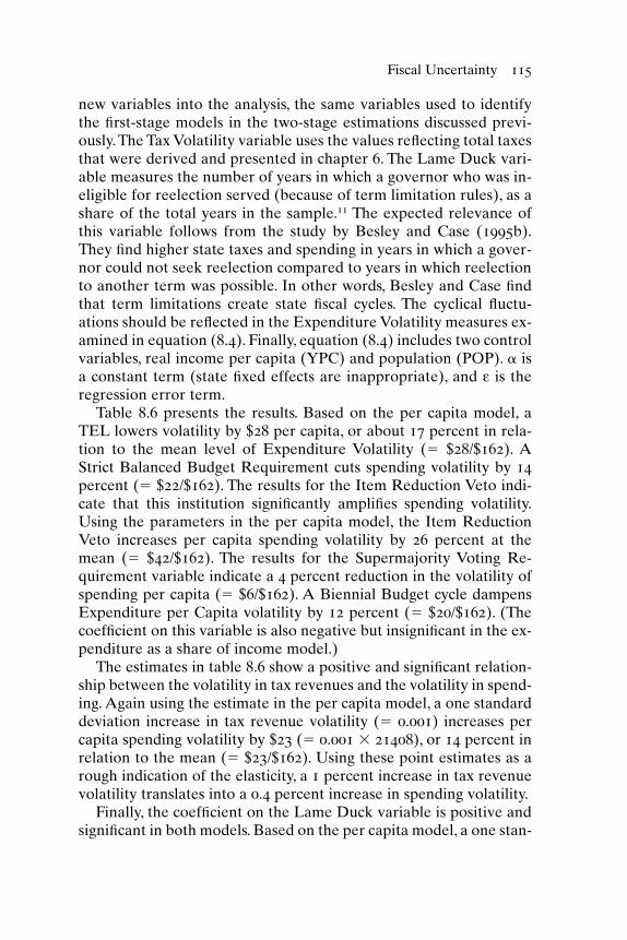
new variables into the analysis, the same variables used to identifythe Arst-stage models in the two-stage estimations discussed previ-ously.The Tax Volatility variable uses the values reBecting total taxesthat were derived and presented in chapter 6. The Lame Duck vari-able measures the number of years in which a governor who was in-eligible for reelection served (because of term limitation rules), as ashare of the total years in the sample.11 The expected relevance ofthis variable follows from the study by Besley and Case (1995b).They And higher state taxes and spending in years in which a gover-nor could not seek reelection compared to years in which reelectionto another term was possible. In other words, Besley and Case Andthat term limitations create state Ascal cycles. The cyclical Buctu-ations should be reBected in the Expenditure Volatility measures ex-amined in equation (8.4). Finally, equation (8.4) includes two controlvariables, real income per capita (YPC) and population (POP). isa constant term (state Axed effects are inappropriate), and ε is theregression error term.
Table 8.6 presents the results. Based on the per capita model, aTEL lowers volatility by $28 per capita, or about 17 percent in rela-tion to the mean level of Expenditure Volatility (� $28/$162). AStrict Balanced Budget Requirement cuts spending volatility by 14percent (� $22/$162). The results for the Item Reduction Veto indi-cate that this institution signiAcantly ampliAes spending volatility.Using the parameters in the per capita model, the Item ReductionVeto increases per capita spending volatility by 26 percent at themean (� $42/$162). The results for the Supermajority Voting Re-quirement variable indicate a 4 percent reduction in the volatility ofspending per capita (� $6/$162). A Biennial Budget cycle dampensExpenditure per Capita volatility by 12 percent (� $20/$162). (ThecoefAcient on this variable is also negative but insigniAcant in the ex-penditure as a share of income model.)
The estimates in table 8.6 show a positive and signiAcant relation-ship between the volatility in tax revenues and the volatility in spend-ing. Again using the estimate in the per capita model, a one standarddeviation increase in tax revenue volatility (� 0.001) increases percapita spending volatility by $23 (� 0.001 � 21408), or 14 percent inrelation to the mean (� $23/$162). Using these point estimates as arough indication of the elasticity, a 1 percent increase in tax revenuevolatility translates into a 0.4 percent increase in spending volatility.
Finally, the coefAcient on the Lame Duck variable is positive andsigniAcant in both models. Based on the per capita model, a one stan-
Fiscal Uncertainty 115
dard deviation increase in the share of Lame Duck years (� 0.29)increases per capita spending volatility by about $5 (� 28 � 0.17), a 3percent increase in relation to the mean (� $5/$162).
Commentary
This chapter exposits a straightforward theme: uncertainty is theenemy of efAciency in public as well as private enterprise. Budgetvolatility precludes efAcient planning and adds signiAcantly to thecost of government-provided services. Put differently, a reduction inspending volatility would be equivalent to a funding increase. Theempirical evidence indicates that a 10 percent reduction in budget
116 Volatile States
TABLE 8.6. Effects of Institutions and Tax Revenue Volatility on State SpendingVolatility
Dependent Variable � Dependent Variable �Volatility in Expenditures Volatility in Expenditures
Independent Variables per Capitaa as a Share of Incomea
Note: Parameters are estimated using robust standard errors. t-statistics are shown in parentheses.aExpenditure Volatility is measured as the standard deviation in the regression residuals from the core
model in equation (8.1).bSee the derivation of the Tax Revenue Volatility variable in chapter 6.cAlaska, Hawaii, and Wyoming are omitted.* Indicates significance at the 5 percent level for a two-tailed test. ** Indicates significance at the 1 percent
level for a two-tailed test.
volatility generates efAciency gains comparable to a 3.5 percent in-crease in the level of funding.
The trade-off between volatility and efAciency means that the roleof Ascal institutions is more complex than previous analysis has gen-erally assumed. Some institutions carry a dual role, exerting not onlya direct inBuence on spending but also an indirect inBuence on thesize of state budgets via their impact on Ascal stability. Consider forexample a Strict Balanced Budget Requirement. The results in table8.2 indicate that this institution cuts per capita spending directly by 3percent. In addition, a Strict Balanced Budget Requirement dampensspending volatility by 14 percent (based on the estimates shown intable 8.6).This 14 percent reduction in spending volatility in turn leadsto an additional 5 percent reduction in per capita spending. In essence,a Strict Balanced Budget Requirement lowers state spending by acombined 8 percent through these two channels.
Consideration of the indirect effects on Ascal institutions is particu-larly important in the analysis of TELs. The results in this chapter andthose in prior studies (e.g., Shadbegian 1996) suggest that the directeffect of TELs diminishes in high income or rapidly growing states.But TELs contribute noticeably to budget stability, reducing spend-ing volatility by 17 percent on average. Through that indirect channelTELs predictably reduce per capita spending by roughly 6 percent.
The analysis suggests that the reliability of tax revenues inBuencesthe size of government. Greater instability in tax revenues con-tributes to spending instability that impedes the efAciency of long-run state government operations. With less efAcient planning, thelevel of government spending increases, which of course requires ad-ditional revenues.
In his 1997 comprehensive survey of the studies of state budget in-stitutions James Poterba concludes that, while the evidence is not con-clusive, the preponderance of studies suggests that institutions are notsimply veils pierced by voters but important constraints on the natureof political bargaining. In essence, the demand for public spending ismediated through a set of Ascal and budget rules. The results in thischapter add fuel to Poterba’s assessment that “Ascal institutions mat-ter.” With a new emphasis on Ascal volatility, institutions appear tomatter more than past research has appreciated.
This goes beyond the Ascal rules assessed explicitly in this chaptersuch as the length of the budget cycle and tax and expenditure limita-tions. For example, Gilligan and Krehbeil (1989) develop a theoreticalframework to assess the relationship between alternative legislative
Fiscal Uncertainty 117
structures and policy uncertainty. They conclude that legislatures withradically majoritarian structures—those that permit very little powerdelegation or agenda control to specialists in committees—generatewider policy variations than legislatures that delegate control to spe-cialized committees. Their analysis also implies that the choice oflegislative procedures (e.g., the use of open versus closed rules foramending policies proposed by committees) may depend on the un-certainty of the policy environment. In other words, a host of alterna-tive legislative and constitutional arrangements are likely to be inter-connected with policy volatility, and the Andings in this chapter stressthe importance of studying these relationships in further detail.
Appendix
118 Volatile States
TABLE 8.A1. Summary Statistics and Data Sources
StandardVariable Mean Median Deviation
Expenditure per Capitaa $2,724 $2,648 $722Expenditure/State Personal Incomeb 12.5% 12.3% 2.5%Revenue per Capitaa $2,958 $2,865 $841Revenue/State Personal Incomeb 13.5% 13.3% 2.9%Total Taxes per Capitaa $1,178 $1,134 $332Total Taxes/State Personal Incomeb 5.4% 5.4% 1.1%Expenditure Volatility (Exp. per Capita) $162 $149 $68Expenditure Volatility (Exp./Income) 0.7% 0.6% 0.3%Tax Revenue Volatility (Tax Rev./
Income) 0.3% 0.3% 0.1%Lame Duck Governor (% of years)c 26% 20% 28%Income per Capitaa $21,983 $21,512 $4,252Unemployment Rated 6.2% 5.9% 2.1%ln (Population)b 15.0 15.1 1.0Urban Population (% of population)b 65% 67% 22%Population Age 18 to 64 (% of
population)b 60% 60% 3%
aDenominated in real (2000) dollars. Data from U.S. Bureau of the Census Web Site.bData from U.S. Bureau of the Census Web Site.cData from Council of State Governments (Biennial Editions, 1968 through 2000), Duncan and
Lawrence (Biennial Editions, 1968 through 2000), Barone and Sujifusa (Biennial Editions, 1968through 2000), and correspondence with state election officials.
dData from U.S. Bureau of Labor Statistics Web Site.