Fish abundance and climate trends in New Zealand -...

New Zealand Aquatic Environment and Biodiversity

Report No. 31 2009

ISSN 1176-9440 Fish abundance and climate trends in New Zealand Matthew Dunn Rosie Hurst Jim Renwick Chris Francis Jennifer Devine Andy McKenzie

Fish abundance and climate trends in New Zealand

Matthew Dunn Rosie Hurst Jim Renwick Chris Francis

Jennifer Devine Andy McKenzie

NIWA PO Box 14−901

Wellington

New Zealand Aquatic Environment and Biodiversity Report No. 31 2009

Published by Ministry of Fisheries Wellington

2009

ISSN 1176-9440

© Ministry of Fisheries

2009

Citation: Dunn, M.R.; Hurst, R.J.; Renwick, J.; Francis, R.I.C.C.; Devine, J.; McKenzie, A. (2009).

Fish abundance and climate trends in New Zealand. New Zealand Aquatic Environment and Biodiversity Report No. 31. 75 p.

This series continues the Marine Biodiversity Biosecurity Report series

which ceased with No. 7 in February 2005.

3

EXECUTIVE SUMMARY Dunn, M.R.; Hurst, R.J.; Renwick J.; Francis, R.I.C.C.; Devine, J.; McKenzie, A. (2009). Fish abundance and climate trends in New Zealand. New Zealand Aquatic Environment and Biodiversity Report No.31. 75 p. Potential correlations between environmental or climate indices and fish stock abundance or year class strength (YCS) have previously been identified for New Zealand stocks of hoki, snapper, red cod, gemfish, rock lobster, and southern blue whiting. In this study we examined a wide selection of fish stock and environmental or climate indices to see if any other similar potential correlations could be found. A total of 212 YCS and annual biomass indices were collated for 56 predominantly commercial finfish species, and 20 climate indices were estimated. The YCS estimates were derived from trawl survey time series, stock assessment models, and standardised catch per unit effort (CPUE) analyses. The biomass indices were derived from research trawl survey time series and standardised CPUE analyses. The fisheries indices had a length of between 5 and 31 years, and the climate indices between 8 and 33 years. Correlations and association tests between the fish YCS or biomass indices and the climate indices were made after predictor screening, restricting data to appropriate times of year, and adding appropriate time lags for YCS indices. Significant (at the 5% level) rank correlations were detected for 21 of the 48 YCS series (44%) and 86 of the 172 biomass series (50%). Significant (at the 5% level) association tests were detected for 34 YCS (71%) and 108 biomass series (63%). Many of the correlations between climate and YCS or biomass indices were as strong as, or stronger than, those routinely reported in the published scientific literature. Potentially interesting correlations were found for several species and stocks. These included school shark, elephantfish, red gurnard, stargazer, hake, and tarakihi. For the Chatham Rise and subantarctic, there were groups of species with markedly similar biomass trends, which in some cases were significantly correlated with climate. These included oblique banded rattail, Bollons’s rattail, and ling on the Chatham Rise, and banded rattail, Oliver’s rattail, dark ghost shark, and pale ghost shark in the subantarctic. There was no clear evidence for any consistent changes in the YCS or relative abundance of species that were classified as ‘warm’ or ‘cold’ water species, and no consistent relationship between these and climate. The correlations identified could nevertheless be spurious, and therefore further investigation is required to establish their validity. Priority should be given to extending existing time series of data, and estimating further appropriate environmental or climate indices on finer and more appropriate spatial or temporal scales. Future analyses might focus on the species identified above, and consider the uncertainty in YCS or biomass indices, other factors that may have affected abundance (e.g., fishing), smaller-scale temporal and spatial variability, and should include a robust statistical analysis of potential climate-fisheries relationships.

4

1. INTRODUCTION The significance of climatic and environmental variability on fisheries productivity has been recognised for many years (e.g., Johnson & Smith 1965), but has grown in prominence more recently, especially with the recognition that human activities may be causing climate change on a global scale (IPCC 2007, Willis et al. 2007a). In New Zealand, there is a rapidly growing body of scientific literature examining the relationship between fisheries and climate. McDowall (1992) considered the potential effect of climate change on freshwater fishes in New Zealand. The potential effect on New Zealand marine fisheries was the subject of a Climate Change Programme Impacts Working Group in 1989 (unpublished report 1989). The working group concluded that predictions of future regional climate were very uncertain, and they therefore made only general predictions for changes to the fisheries under a number of potential climate scenarios. The predicted impacts on fish populations were of two main types: (1) shifts in spatial distribution, and (2) changes to reproductive success and growth (i.e., productivity). The working group concluded that shifts in distribution would be more pronounced than changes in productivity, at least initially. This conclusion was consistent with more recent reports with a similar scope (e.g., Hobday et al. 2006). The potential effects that climatic variability may have on fish are undoubtedly complex (Brander 2007). Being ectotherms (“cold blooded”), the physiological processes of fishes, such as their respiration and activity rate, growth and maturation, and sex determination, are directly influenced by temperature (Myers 2001, Devlin & Nagahama 2002, Pörtner et al. 2008). Changes in temperature have also been shown to change fish behaviour, such as migration routes (Stensholt 2001). There may also be indirect effects of climate change on fishes through changes in the availability of their food or habitat (Cushing 1990, Beaugrand et al. 2003, Otterson et al. 1994, Heath 2005). This can take place through, for example, changes in the location of productive frontal zones where the currents mix and their prey congregate (Zainuddin et al. 2008), the degree to which water columns mix because of wind direction and strength (Zeldis et al. 2005), or the composition of the plankton (Reid et al. 2001, Beaugrand 2004). All fishes can tolerate a range of environmental conditions, although the limits of what they can tolerate depends on species, and potentially even on the population in question (Pörtner et al. 2008). Some species seem to be able to withstand and potentially adapt to a wide range of environmental and climatic conditions, at least for some of the time (Neat & Righton 2007). For the sustainability of fisheries on these species, overfishing may be a more immediate and greater problem, although more extreme environmental conditions certainly don’t seem to help (O’Brien et al. 2000, Rothschild 2000, Brander 2005). When abrupt climatic changes take place they can often have a much more dramatic effect. These are sometimes referred to as “regime shifts”. Such a regime shift took place in the North Sea in the late 1980s and early 1990s, at which time water currents and sea temperatures changed, and caused changes in the distribution and abundance of plankton, benthic invertebrates, and many species of fish (Reid et al. 2001, Beaugrand 2004, Dulvy et al. 2008). Some of these fish species were commercially exploited, so as a result the local fisheries also had to change (ICES 2004a, 2004b). Despite the pervasive influence of the climate on fish life history, many studies only establish statistical correlations between large-scale environmental indices and fish abundance or distribution. As a result the mechanism behind the correlation is usually untested. In doing so, there is always a risk that the correlation was incorrect, or aliasing for something else, and the correlation might be misleading (Francis 2006). The environmental indices used in this way have been varied, for example temperature, light levels, salinity, oxygen levels, turbulence, and advection (e.g., Otterson et al. 2006, Stige et al. 2006, Roselund & Halldórsson 2007).

5

Nevertheless, identifying large-scale correlations is a first step towards identifying which species may be most at risk from environmental variability and climate change, knowing how many species in an area might be potentially vulnerable, the rate at which changes might occur, and perhaps which species might be at risk of local extinction (Perry et al. 2005, Rose 2005, Hannessonn 2007). This has obvious value for fisheries management, by allowing changes in fish stocks to be better understood, and allowing the various threats to fish stocks to be better evaluated (Schiermeier 2004). 1.1 Existing case studies in New Zealand Hoki (Macruronus novaezelandiae) is one of the most valuable fisheries in New Zealand. In the early 2000s the hoki catch biomass declined, and the catch quota was substantially reduced. Although factors such as over-exploitation or intensive fishing on spawning aggregations may have contributed to the decline, poor recruitment for a period of 7 years (1995–2001) was a contributing factor. It is possible that climatic conditions in the mid 1990s to early 2000s may have been detrimental to recruitment. A relationship between climate and recruitment was found by Bull & Livingston (2001), but as the time series available for analysis increased the relationship became less clear (Francis et al. 2006). In the most recent study, Francis et al. (2006) used revised estimates of year class strength (YCS), and found that a generalised linear model (GLM) with YCS as the predictand and between 1 and 5 climate predictors, gave little or no predictive ability for YCS. The main reason for the change in result would appear to be the revision of the YCS estimates, as those used by Francis et al. (2006) were substantially different from those used by Bull & Livingston (2001). Francis et al. (2006) suggested three reasons for their failure to detect a relationship between climate and hoki YCS: that the “right” environmental predictors were not included, that the environment-recruitment relationship may be more complex than described by the GLM, or that the environment-recruitment hypotheses were simply wrong. Additional reasons could be that the assumptions about stock structure could be wrong, or that the relationship between YCS and climate changed as the hoki stocks were depleted (Brander 2005). There are a number of hypotheses for how climate may affect hoki recruitment. Bull & Livingston (2001) suggested stronger winds might cause increased upwelling in coastal areas, which might increase primary and secondary productivity and therefore food supply for hoki post-larvae, as well as facilitating the inshore transport of post-larvae towards the high food density areas; together these might improve growth and survival and lead to a higher YCS. They also suggested that the abundance of strong year classes might force weaker year classes to occupy more marginal habitat, which might exacerbate YCS variability. Francis et al. (2006) discussed the first hypothesis further, suggesting climate may also affect the timing of the water column mixing and subsequent productivity (a “match-mismatch hypothesis”, Cushing (1990)). Beentjes & Renwick (2001) found that the recruitment of red cod (Pseudophycis bachus) was relatively high during colder years, which were associated with the El Niño events. The red cod fishery was dominated by new recruits, and therefore predicting recruitment was essentially the same as predicting potential fishery yield. A linear model relating catch to sea surface temperature has therefore been used to explain patterns in historical catches, and to forecast potential catches 1 year ahead, with some confidence (Beentjes & Renwick, pers.comm.). Relatively high recruitment and faster growth rates of snapper (Pagrus auratus) in the Hauraki Gulf (snapper stock SNA 1) have been correlated with warmer conditions (Francis 1994a). The strength of the correlation between sea surface temperature (SST) and snapper year class strength depended on the months used for estimating SST, with the correlation increasing in December, peaking in February, and remaining high until June (Francis 1993).

6

This plateau corresponded with the end of larval settlement, settlement, and early post-settlement. SST was also found to affect larval duration, with higher temperatures reducing the time in the plankton, leading to earlier settlement and metamorphosis (Francis 1994b). Gilbert & Taylor (2001) found similar correlations between YCS and sea temperature for snapper stocks on the east coast of the North Island (SNA 2) and west coast South Island (SNA 7). Zeldis et al. (2005) found upwelling favourable winds caused increased incursions of shelf water into the Hauraki Gulf, which correlated with greater surface mixing, primary productivity, abundance of zooplankton, and higher survival of larval snapper. Zeldis et al. hypothesised that the higher survival rates of larval snapper might have been a response to improved feeding and growth conditions, and noted that this effect might be in addition to the direct temperature effects identified by Francis (1994b). Fluctuations in the recruitment of gemfish (Rexea solandri) on the west coast of the South Island (WCSI), when classified as either “high” or “low” YCS, appeared to be negatively correlated with the winter frequency of occurrence of the south westerly wind flow, and positively correlated to the SST (Renwick et al. 1998). Increased southwesterly flow was consistent with lower SST, as the increased mixing would enhance heat flux out of the ocean. Renwick et al. (1998) hypothesised that the reduced recruitment in colder years was because of temperature sensitivity, as gemfish reached the southern limit of their range on the WCSI. They also noted that the pattern of YCS for gemfish was roughly opposite that for hoki YCS over the same time period. Booth et al. (2000) developed a linear regression model that estimated rock lobster (Jasus edwardsii) puerulus settlement from two predictors, the Kidson “Trough” regime and a “High over the southeast” weather class. This implied that southerly stormy weather leads to increased settlement rates, but the mechanism involved remained unresolved, and no hypotheses were given. The authors concluded that the Wairarapa Counter Current might also have an effect on settlement. Hanchet & Renwick (1999) found correlations between southern blue whiting (Micromesistius australis) YCS in the subantarctic and winter air pressure over the Campbell Plateau, the Kidson “Trough” index in summer, and the Hokitika – Chathams air pressure difference. A linear regression with these predictors had weak predictive ability, but an alternative analysis on the same data using YCS categories (“weak”, “medium”, and “strong”) proved to have a greater predictive ability, correctly classifying 76% of YCS in a cross-validation procedure. This model predicted YCS using the Auckland – Christchurch air pressure difference, SST near Campbell Island, and an index of the “Ridge across South Island” weather type. In general, the correlations suggested southern blue whiting YCS was greater in years with less stable, cooler ocean conditions. Willis et al. (2007b) found negative correlations between southern blue whiting YCS in the subantarctic and the presence of a large high pressure system over the Campbell Plateau in winter, or a high pressure system over the northwest which would result in strong winds over the subantarctic in spring. They also found no significant correlation between YCS and SST, and hypothesised that higher YCS might result from rough winters with a high degree of water column mixing, following by relatively calm spring conditions. This supports the conclusions of Hanchet & Renwick (1999). Although the Willis et al. analyses showed a good correlation between some climatic variables and YCS, the linear regression models tended to underestimate very strong YCS and overestimate very weak YCS. Willis et al. suggested this was probably because the predictors described patterns over larger spatial scales than that at which the biological processes determining YCS operated. Alternatively, the relationship between climatic variables and YCS may become highly non-linear when climatic conditions outside the ‘norm’ are encountered. There are a number of other studies which have less directly considered the climate effects on fisheries. Ayers et al. (2006) reviewed information for school sharks (Galeorhinus australis)

7

around New Zealand, focusing on catch per unit effort (CPUE) indices of biomass. They hypothesised that there was a single population, which undertook north-south migrations depending on SST, with warmer years favouring a southerly movement. Taylor (2001) included a wind speed predictor in subantarctic orange roughy (Hoplostethus atlanticus) standardised CPUE models, after it was hypothesised that high wind speed led to low CPUE (and vice versa), in other words to a reduction in catchability; this was considered a particular problem for subantarctic fisheries. Although the wind speed predictor was statistically significant in the final CPUE model, it did not have any appreciable effect on the final CPUE index, and the model estimated relationship between CPUE and wind speed was not described. Neumann (2001) correlated SST with the distribution of dolphins (Delphinus delphis), which moved closer inshore during warmer years. Taylor (2002) described the invasion of the Chilean jack mackerel (Trachurus murphyi) into New Zealand waters in the mid 1980s, a species which subsequently dominated the jack mackerel fishery in some areas. The timing of this event coincided with increased frequency and magnitude of El Niño (Elizarov et al. 1993). Determining potential correlations between fisheries and climate indices, rather than causal mechanisms, has been the focus of studies in New Zealand (and for most studies elsewhere). The investigations on snapper have come closest to understanding the causal mechanisms. The climate indices most frequently identified in the relationships were SST, pressure differences, wind strength and direction, and broad measures of climate (e.g., the Kidson regime indices; note that “regime” here has a climate-specific meaning, and is different from the ecological “regime shifts” described for the North Sea earlier). In addition, most of the New Zealand studies have focused on determining climate effects on YCS, rather than on distribution and catchability, even though climate effects on distribution might be more pronounced and therefore easier to detect. Francis et al. (2003) found significant evidence of inter-annual variation in catchability in trawl surveys and commercial fishery CPUE, and noted that this could be caused by changes in the distribution of the fish stocks, but considered the data series too short to allow examination of any causative factors. 1.2 Scope of the present study The work described in this report was carried out under Ministry of Fisheries project SAM2005/02, with the specific objective “To examine the possible effects of climate on fishery yields and abundance indices for commercial fisheries around New Zealand”. The approach taken was to search for possible correlations between a wide range of environmental and fisheries indices, as well as focus on some specific species and areas where data sets were most extensive and reliable, and where a priori we might most expect to see climate effects. We focused on coastal and middle depth finfish species. The wide range of stock indices (N=212) and climate indices (N=20) precluded the detailed examination of individual potential relationships; this is left to future studies. The strength of this approach was that it examined a wide range of stocks. Some of these were of short-lived species; variability in stock biomass caused by climate sensitivity is more likely to be seen in highly productive and short-lived species, because such variability will be effectively hidden in the extended age-structure of longer-lived species. We also examined both YCS and catchability (distributional) correlations. Rapid changes in stock abundance are likely to be associated with major oceanographic changes, or fisheries exploitation (which may include catch levels and catchability effects). We also considered species with a more southern (cold water) or northern (warm water) distribution; we might expect the most obvious changes in biomass and productivity to be in stocks which are located near the limits of their geographic range, where the physiological limits are being approached.

8

There are clearly some limitations on the conclusions that we can draw from this approach. The scale over which the climate indices are measured is usually far removed from the scale over which most biological processes are taking place, and therefore possible causative factors behind correlations remain speculative. Also, the absence of a correlation does not necessarily mean that climate does not have a large effect on a stock. For example, we might not have the “right” climate indices, or the strength and nature of correlations might not be constant where large changes in species’ abundance or life history have taken place (e.g., age structure, Longhurst (2002), Brander (2005)). Finally, many time series used in this study are relatively short, and must be interpreted with caution. Over a short time period, random variability might easily look like a trend, and might appear to be significantly correlated with climate (Francis 2006). 2. METHODS 2.1 Environmental data The environmental and climate indices used here included most of those used in previous New Zealand climate and fisheries studies. We also included relatively new indices for sea surface height, and sea surface colour. Plots of all of the environmental and climate indices are given in Appendix A. The environmental indices used in this study cover a range of time scales. The “Kidson weather types” and “Trenberth” indices both describe New Zealand-local climate variations. A significant fraction of the variability is associated with weather events and is hence unpredictable, or random, on monthly and longer time scales. The Kidson weather types are defined on a 12-hourly basis, describing the daily sequence of weather over New Zealand in terms of a set of 12 types of weather maps, or surface wind flows. For this research, the monthly and longer frequency of occurrence of each of the types was used, to describe the character of a given month or season in terms of the representative types. Further to this, the 12 weather type frequencies may be grouped into the frequencies of occurrence of three weather “regimes”, associated with westerly air flows, settled anticyclonic (reduced westerly) conditions, and with disturbed weather patterns. The Trenberth indices describe monthly mean differences in mean sea-level pressure between various climate stations in the New Zealand region. Pressure differences are directly related to wind speed (perpendicular to the orientation of the pressure difference), hence the Trenberth indices encapsulate monthly mean wind flow direction and speed over New Zealand. As such, they are well correlated with some of the monthly Kidson weather type and regime frequencies, which also capture wind flows and pressure patterns around New Zealand (Table 1). Wind and pressure patterns affect surface ocean conditions through heat flux, degree of surface mixing, and upwelling on exposed coasts. However, large-scale climate signals do modulate surface climate over New Zealand. The El Niño-Southern Oscillation (ENSO) cycle in the tropical Pacific has a strong influence on New Zealand. ENSO is described here by the Southern Oscillation Index (SOI), a measure of the difference in mean sea-level pressure between Tahiti (east Pacific) and Darwin (west Pacific). When the SOI is strongly positive, a La Niña event is taking place. New Zealand tends to experience reduced westerly winds and milder, more settled, anticyclonic weather. When the SOI is strongly negative, an El Niño event is taking place. New Zealand tends to experience increased westerly winds and cooler, less settled weather. Causal relationships of correlations of SOI with fisheries processes will be obscure, but probably related to one or more of the underlying ocean climate processes such as winds or temperatures. The ENSO cycle is irregular, with El Niño events occurring every 3 to 7 years. There are no indications of long-term trends in the ENSO cycle (associated with anthropogenic climate

9

change, or other causes), and future climate change projections give no strong indications of ENSO trends in future. The ENSO cycle is, however, naturally modulated by the Interdecadal Pacific Oscillation (IPO), a Pacific-wide reorganisation of the heat content of the upper ocean. The IPO changes from its positive to its negative polarity every 20 to 30 years. In the positive polarity, El Niño events tend to be more frequent and stronger, while in the negative polarity, El Niño events are weaker, and La Niña events are more prominent. Hence, New Zealand tends to experience 20–30 year periods of enhanced and reduced westerlies, with associated temperature and precipitation effects. There do not appear to be long-term trends in the behaviour of the IPO (or of ENSO) at present. However, paleoclimate evidence shows that over the past several thousand years, there have been centuries-long periods of little or no ENSO activity, and periods of strong and regular ENSO activity. The causes of such behaviour, and its implications for the future, are current research questions. Sea surface temperature (SST) measures temperature at the very surface (less than 1 mm when measured from satellites). It may therefore not represent the temperature of the ocean as a whole. Sea surface height (SSH) is measured from satellites, and a better measure of temperature throughout the water column, with higher mean sea surface height indicating an increase in temperature. However, SST and SSH are quite closely correlated (Table 1). Sea temperatures are obviously influenced by weather conditions, and are reasonably well correlated with weather indices such as the SOI, and the Kidson “Blocking” regime (Table 1). Water temperatures directly affect fish, and have been found to be correlated with a variety of fisheries processes. The level of primary productivity can be inferred from measurements of sea surface colour made from satellites. In coastal areas higher surface colour indicates higher chlorophyll concentrations (i.e., biomass of green algae), as well as the levels of suspended particles and dissolved organic matter. In oceanic areas the main source of colour is chlorophyll. Higher chlorophyll concentrations indicate higher ecosystem productivity. Higher primary productivity potentially has a more direct link to fisheries process than climate indices. The weather type frequencies and pressure indices are both related to surface ocean conditions, largely through implied surface ocean heat fluxes. More settled, low-wind periods tend to be associated with increased sea temperatures, while the windier more disturbed flows tend to be associated with cooler seas. Coastal upwelling is modulated by along-shore wind flows, hence there are relationships between the various weather types and wind flows and upwelling on exposed coasts. Further and more detailed climate and environmental indices of relevance to fisheries are being described for Ministry of Fisheries project ENV2007/04. 2.1.1 Kidson regime indices The Kidson regimes (Kidson 2000) relate to the occurrence of different types of weather pattern over New Zealand. Kidson (2000) developed 12 weather patterns that describe the day to day variability in the atmospheric circulation and weather over the country. These were further grouped into three regimes, labelled Trough, Zonal, and Blocking. The “Trough” Kidson regime is characterised by pressure troughs over and east of the country. It is linked with high rainfall, and below-normal temperatures in the south. The Trough regime typically brings wet, cool, and cloudy conditions to most of the country. The “Zonal” Kidson regime is characterised by intense anticyclones north of 40° S, and strong westerlies to the south of the country. This produces an intensified westerly gradient south of the country, with highs to the north. The Zonal regime is linked with below-normal rainfall in the north and east, and above-normal temperatures in the south.

10

Tab

le 1

: Pea

rson

cor

rela

tion

coef

ficie

nts f

or p

aire

d co

rrel

atio

ns o

f ann

ual m

ean

estim

ates

of t

he e

nvir

onm

enta

l ind

ices

. K

idso

nch

loro

phyl

lss

t by

FMA

ssh

by F

MA

Z1Z2

Z3Z4

M1

M2

M3

ZNZS

MZ1

MZ2

MZ3

MZ4

SOI

TrZo

BlW

CSI

Sub

AC

hat

12

34

56

78

91

23

45

67

89

Z11

Z20.

528

1Z3

0.95

60.

633

1Z4

0.73

70.

221

0.65

91

M1

-0.1

80.

006

-0.1

3-0

.17

1M

20.

487

0.31

90.

422

0.77

4-0

.04

1M

3-0

.21

-0.0

1-0

.15

-0.2

10.

998

-0.1

1ZN

0.95

60.

446

0.91

30.

852

-0.1

70.

573

-0.2

1ZS

0.78

20.

710.

907

0.34

-0.0

60.

19-0

.07

0.65

61

MZ1

0.24

2-0

.09

0.29

8-0

.10.

01-0

.58

0.04

30.

196

0.34

81

MZ2

0.79

50.

653

0.91

0.32

7-0

.05

0.09

9-0

.06

0.68

60.

974

0.49

31

MZ3

0.73

0.34

80.

667

0.91

-0.0

70.

913

-0.1

30.

812

0.39

6-0

.22

0.35

1M

Z40.

792

0.17

60.

696

0.83

9-0

.24

0.55

3-0

.27

0.88

40.

375

0.08

40.

397

0.72

81

SO

I-0

.42

-0.1

6-0

.3-0

.49

0.02

3-0

.48

0.05

-0.4

3-0

.11

0.25

7-0

.06

-0.5

1-0

.41

1K

idso

nTr

0.30

6-0

.36

0.2

0.68

2-0

.18

0.39

5-0

.20.

439

-0.0

8-0

-0.0

90.

509

0.62

1-0

.24

1Zo

0.49

40.

787

0.53

50.

134

0.01

30.

229

1E-0

40.

369

0.60

7-0

.02

0.58

10.

270.

088

-0.3

1-0

.51

1B

l-0

.8-0

.38

-0.7

3-0

.85

0.17

8-0

.64

0.21

4-0

.82

-0.5

0.02

2-0

.47

-0.8

-0.7

40.

554

-0.5

6-0

.42

1C

hlor

ophy

llW

CSI

0.62

30.

415

0.58

50.

647

-0.1

60.

545

-0.1

70.

626

0.37

7-0

.19

0.30

90.

622

0.4

-0.8

60.

341

0.30

3-0

.71.

00S

ubA

-0.2

-0.6

8-0

.40.

228

-0.4

0.44

8-0

.41

-0.1

-0.7

1-0

.77

-0.8

10.

324

0.2

-0.3

30.

629

-0.7

-0.3

1-0

.02

1.00

Cha

t-0

.32

0.20

1-0

.2-0

.63

0.11

1-0

.66

0.13

1-0

.31

0.00

50.

684

0.22

8-0

.6-0

.45

0.73

-0.6

0.48

50.

44-0

.38

-0.3

81.

00ss

t by

FMA

1-0

.13

0.26

60.

053

-0.4

30.

043

-0.4

0.06

5-0

.21

0.31

40.

257

0.33

6-0

.39

-0.3

90.

561

-0.4

80.

098

0.41

6-0

.34

-0.7

90.

451

2-0

.21

0.23

2-0

.05

-0.3

70.

01-0

.40.

033

-0.2

50.

161

0.10

70.

162

-0.4

3-0

.33

0.44

9-0

.30.

034

0.28

1-0

.78

-0.3

80.

340.

837

13

-0.4

8-0

.16

-0.3

2-0

.49

0.10

9-0

.30.

125

-0.4

9-0

.09

-0.0

5-0

.1-0

.45

-0.5

0.51

3-0

.33

-0.2

0.53

9-0

.84

-0.0

70.

420.

560.

515

14

-0.4

5-0

.15

-0.3

-0.5

70.

057

-0.5

0.08

5-0

.49

-0.0

40.

103

-0.0

3-0

.59

-0.5

0.61

3-0

.34

-0.2

20.

573

-0.8

8-0

.10

0.46

0.70

10.

730.

881

5-0

.47

-0.1

6-0

.33

-0.5

20.

032

-0.3

0.04

9-0

.51

-0.0

9-0

.07

-0.1

2-0

.43

-0.5

70.

402

-0.3

1-0

.15

0.48

-0.9

10.

130.

370.

577

0.58

90.

880.

81

6-0

.2-0

.25

-0.1

7-0

.34

0.03

-0.1

40.

038

-0.2

9-0

.01

-0.0

2-0

.06

-0.2

-0.3

0.05

4-0

.14

-0.1

40.

283

-0.5

70.

64-0

.07

0.27

20.

230.

610.

580.

721

7-0

.52

-0.1

1-0

.35

-0.6

50.

169

-0.4

50.

194

-0.5

7-0

.07

0.06

6-0

.06

-0.5

8-0

.60.

645

-0.4

4-0

.19

0.64

7-0

.79

-0.2

70.

450.

756

0.68

40.

890.

90.

870.

531

8-0

.41

0.02

9-0

.23

-0.6

30.

195

-0.5

10.

223

-0.4

80.

057

0.14

80.

07-0

.6-0

.53

0.61

4-0

.47

-0.0

80.

572

-0.7

0-0

.48

0.42

0.87

80.

846

0.77

0.89

0.75

0.44

0.93

19

-0.3

20.

106

-0.1

3-0

.56

0.10

7-0

.46

0.13

2-0

.39

0.15

90.

176

0.17

9-0

.52

-0.5

20.

631

-0.5

2-0

.01

0.55

7-0

.47

-0.7

10.

500.

951

0.79

50.

740.

830.

70.

350.

890.

951

ssh

by F

MA

1-0

.24

0.19

70.

062

-0.4

4-0

.05

-0.1

9-0

.04

-0.2

70.

390.

033

0.34

5-0

.31

-0.4

30.

687

-0.4

3-0

.03

0.64

8-0

.90

-0.3

50.

450.

797

0.75

70.

90.

850.

90.

630.

880.

780.

811.

002

-0.3

40.

236

-0.0

6-0

.54

-0.0

7-0

.34

-0.0

6-0

.39

0.29

20.

022

0.26

2-0

.5-0

.49

0.70

5-0

.52

0.02

80.

718

-0.9

1-0

.25

0.31

0.82

30.

878

0.9

0.92

0.87

0.59

0.88

0.86

0.85

0.94

1.00

3-0

.36

0.27

8-0

.13

-0.5

3-0

.04

-0.1

5-0

.04

-0.4

40.

226

-0.2

20.

142

-0.4

-0.5

20.

592

-0.4

90.

119

0.58

4-0

.90

-0.0

60.

450.

636

0.70

90.

840.

810.

890.

690.

790.

710.

690.

900.

921.

004

-0.3

80.

293

-0.1

2-0

.55

-0.0

5-0

.23

-0.0

4-0

.44

0.22

5-0

.13

0.17

9-0

.45

-0.5

40.

648

-0.5

40.

092

0.67

4-0

.94

-0.1

30.

520.

719

0.79

70.

880.

880.

890.

640.

840.

780.

760.

930.

960.

981.

005

-0.4

0.26

1-0

.14

-0.6

1-0

.03

-0.2

7-0

.02

-0.4

70.

226

-0.1

10.

165

-0.4

9-0

.55

0.68

1-0

.52

0.06

40.

685

-0.9

2-0

.11

0.48

0.67

70.

750.

880.

860.

910.

670.

840.

760.

730.

930.

940.

980.

981.

006

-0.4

60.

229

-0.2

6-0

.63

-0.0

3-0

.27

-0.0

2-0

.55

0.10

2-0

.21

0.02

4-0

.52

-0.5

90.

634

-0.4

90.

033

0.66

9-0

.81

-0.1

00.

410.

570.

676

0.82

0.8

0.86

0.64

0.75

0.66

0.62

0.86

0.88

0.95

0.93

0.97

1.00

7-0

.42

0.23

5-0

.13

-0.6

10.

013

-0.2

90.

024

-0.4

50.

241

-0.0

30.

215

-0.4

9-0

.56

0.73

9-0

.54

0.04

10.

734

-0.9

4-0

.18

0.57

0.76

30.

819

0.94

0.91

0.92

0.63

0.92

0.84

0.81

0.96

0.96

0.94

0.97

0.97

0.91

1.00

8-0

.35

0.22

2-0

.04

-0.5

5-0

.02

-0.2

6-0

.01

-0.3

80.

312

0.01

80.

286

-0.4

3-0

.51

0.73

7-0

.51

0.01

80.

705

-0.9

3-0

.26

0.60

0.78

80.

799

0.93

0.89

0.91

0.61

0.92

0.82

0.82

0.98

0.95

0.93

0.96

0.96

0.89

0.99

1.00

9-0

.30.

267

0.02

6-0

.53

-0.0

2-0

.26

-0.0

1-0

.33

0.38

10.

047

0.35

2-0

.4-0

.49

0.71

4-0

.51

0.04

80.

686

-0.8

9-0

.35

0.63

0.81

0.78

30.

920.

870.

890.

60.

910.

820.

840.

980.

950.

920.

950.

950.

870.

981.

001.

00

11

The “Blocking” Kidson regime is characterised by pressure highs lying to the south and east, and is linked with a southwest-northeast contrast in rainfall (below normal in SW, above normal in NE) and above-normal temperatures, except on the east coast of both islands. These regimes have shown a seasonal pattern, with reduced frequency of the Zonal regime and greater frequency of the Blocking regime over summer. The mean persistence of any regime tends to be about 1–1.8 days, but individual regimes may dominate the weather for 2–4 weeks. It should be noted that the Kidson regimes are not that clearly defined, and within each the variation in climatic elements is large. As a result, in climate studies they are considered only a qualitative measure. The frequencies of these are not strongly linked to larger scale indices, such as the SOI, though the ENSO cycle does modulate weather sequences over New Zealand to a degree. The Kidson indices were supplied as the percentage of days in each month in each of the three Kidson regime types (Trough, Zonal, Blocking). 2.1.2 Mean sea-level pressure indices These indices measure mean sea level pressure differences, which by the geostrophic relationship are proportional to the mean wind speed in wind direction perpendicular to that of the line between the two measurement points. The indices used in this study are the Trenberth indices (Trenberth 1976), and the SOI (e.g. Mullan 1995) (Table 2). The Trenberth indices refer to specific areas of New Zealand, and are just differences in mean sea level pressure between the sites listed. For example, Z1 is the monthly mean sea level pressure difference of Auckland minus Christchurch. They are normalised to be unit standard deviation departures from a mean of zero. By geostrophic balance, the pressure difference between two points is a direct proxy for the average strength of the wind perpendicular to that pressure difference, in the region between the points. So, Z1 measures (approximately) the strength of the westerly wind over the region between Auckland and Christchurch, since the pressure difference is roughly north-south, so the geostrophic wind is roughly east-west. The "Z" indices are for Zonal (i.e., westerly) wind, as they are mostly north-south differences, and are well correlated. The "M" indices are for Meridional (i.e., southerly) wind as they are mostly east-west differences. The "MZ" indices measure winds in the northwest-southeast and southwest-northeast directions. The correlation between the various Trenberth indices is shown in Table 1. The Trenberth indices were available for 1973–2006. The SOI is the normalised mean sea surface pressure difference between Tahiti and Darwin and is related to the strength of the trade winds in the southern hemisphere tropical Pacific. Values of the SOI above 10 indicate La Niña conditions, associated on average with more northeasterlies and warmer temperatures over New Zealand, whereas those below -10 indicate El Niño, associated on average with enhanced southwesterlies and cooler temperatures over New Zealand. The Trenberth index MZ3 is therefore correlated with the SOI but is defined locally over New Zealand rather than in the Tropics. There was one missing value for M1, which was replaced with the mean for the month over all other years. 2.1.3 Sea surface temperature, sea surface height, and primary productivity Sea surface temperature, sea surface height, and sea surface chlorophyll indices were derived from satellite observations (Uddstrom & Oien 1999). Monthly sea surface temperature (SST) was available on a 1° by 1° grid from 160.5° E to 172.5° W and 30.5° S to 58.5° S, for 1973–2006. Monthly sea surface height (SSH) was available on a 1° by 1° grid from 160.5° E to 172.5° W and 30.5° S to 58.5° S, for 1992–2006, and was correlated with SST (Table 1).

12

Monthly mean and anomaly values of chlorophyll were available for three regions, the west coast South Island (WCSI), SubAntarctic (SubA), and Chatham Rise (Chat), for 1997–2004. Table 2: The Trenberth and SOI indices, and the mean wind direction and area to which they apply, with the Fisheries Management Area (FMA) and area to which they were applied in this study (Chat, Chatham Rise; TB, Tasman Bay; WCSI, west coast South Island; SubA, SubAntarctic). Index Mean wind direction and area FMA Area Z1 : Auckland -Christchurch

Westerly, North Island & northern South Island

1,2,3,4,7,8,9 Chat, TB, WCSI

Z2 : Christchurch-Campbell

Westerly, southern South Island & sub-Antarctic

3,4,5,6,7 Chat, WCSI, SubA

Z3 : Auckland-Invercargill

Westerly, whole of New Zealand 1-9 Chat, TB, WCSI, SubA

Z4 : Raoul-Chatham

Westerly, 30-45S 1,2,3,4,7,8,9 Chat, TB, WCSI

M1 : Hobart-Chatham Southerly, Tasman/New Zealand/Chatham Rise

1,2,3,4,7,8,9 Chat, TB, WCSI

M2 : Hokitika-Chatham

Southerly, New Zealand/Chatham Rise

2,3,4 Chat

M3 : Hobart-Hokitika

Southerly, Tasman Sea 7,8,9 TB

MZ1 : Gisborne-Hokitika

Northwesterly, central New Zealand

3,4,7 Chat, WCSI, TB

MZ2 : Gisborne-Invercargill

Northwesterly, southern North Island and South Island

3,5,6,7 WCSI,SubA

MZ3 : New Plymouth-Chatham

Southwesterly, central New Zealand

2,3,4,7,8 Chat,WCSI, TB

MZ4 : Auckland-New Plymouth

Westerly, northern North Island 1,2,8,9 none

ZN : Auckland-Kelburn

Westerly, North Island 1,2,8,9 TB

ZS : –Kelburn-Invercargill

Westerly, South Island 3,4,5,6,7 Chat, WCSI, TB, SubA

SOI : Tahiti-Darwin Northeast/southwest All all 2.2 Fisheries data The fisheries data fell into two groups: 1. Indices of year class strength (YCS) estimated from:

a. Stock assessment model outputs b. Research trawl survey estimates of individual cohort abundance c. Commercial catch per unit effort (CPUE) analyses, where it could be assumed that

the fishery was exploiting only a single cohort (e.g., arrow squid) 2. Indices of relative biomass estimated from:

a. Research trawl surveys b. Commercial CPUE analyses

Tests for correlations between climate and YCS indices effectively assumed that climate can influence spawning success or juvenile mortality rates. Tests for correlations between climate and biomass indices effectively assumed that climate can influence catchability. No assumption was made about the relationship between YCS and biomass. In some instances the same set of observational data could be used several times, for example the Chatham Rise middle-depths

13

trawl survey provided three estimates for hake; 3+ YCS, 4+ YCS, and total biomass (all age classes). The estimates of year class strength (YCS) were taken either from the MFish Stock Assessment Plenary Reports (e.g., Ministry of Fisheries Science Group 2007), or from published Fisheries Assessment Reports (FARs). Most of the YCS estimates were from stock assessment models (HOKe and HOKw), others were cohort specific estimates from trawl survey (e.g., HOK.Chat) or surveys or fisheries which were dominated by a single year class (e.g., WCSI.ASQ) (Table 3). In the last two cases, it was usually necessary to offset the year of the index so that it corresponded to the birth year. YCS estimates from stock assessment models are output as the birth year, and so no year offset was necessary. No allowance was made for potential ageing errors in estimating YCS. For hake, ling, and barracouta, YCS estimates were available for the same year class in subsequent years, e.g., the relative YCS of a cohort was measured at age 3+ in year 1, and then again at age 4+ in year 2. In these cases, the estimates were combined to obtain a single set of YCSs. This combination was done in three steps: (1) the abundance estimates for the older age group were scaled so that they had the same mean value as those for the younger age group (where the means were calculated just for the birth years in which the estimates from the two groups overlapped); (2) a mean YCS was calculated for every birth year with at least one estimate; and (3) these mean YCSs were scaled to average 1. Note that the scaling between age groups will be poor for the two barracouta instances (where there was only one year of overlap), but should be much better for hake and ling, with 7 years of overlap in each case. The indices derived in this way were BAR7TB, BAR7WCm HAK5+6 and LIN5+6 (Table 3). The abundance indices were all expressed in terms of biomass. Biomass indices from trawl surveys and commercial CPUE in the same area may not necessarily show the same patterns, as they could be monitoring different parts of the population. Commercial vessels usually spatially and temporally target their fishing effort, whereas trawl surveys are designed to sample fish populations at random (in a statistical sense). The biomass data were obtained from three main sources: the MFish Fisheries Plenary Report (Ministry of Fisheries Science Group 2007); standardised CPUE indices calculated for species in the Adaptive Management Programme (Paul Starr, pers.comm., May 2007); and estimates from MFish trawl surveys published in FARs, up to October 2006. Where multiple AMP CPUE indices were available, only those considered most reliable and plausible were used in the analyses (Paul Starr, pers.comm., May 2007). The trawl survey indices included unpublished estimates for some of the less abundant or non-commercial species thought to be usefully sampled by a bottom trawl. The precision of the biomass estimates (although collated) were not used in the analyses. Eight trawl surveys were included (Table 4). Indices derived from these trawl surveys were prefixed with the survey label, and had the type “trawl” (Tables 3 & 4). A spawning season (autumn, winter, summer, spring) was defined for each species, where data were available (Table 3). Sources included the Ministry of Fisheries Plenary Report and website on status of the stocks (http://www.fish.govt.nz/en-nz/SOF/default.htm in June 2008), as well as published information summarising trawl surveys and Ministry of Fisheries observer records (Hurst et al. 2000, O’Driscoll et al. 2003). These seasons were used to determine the appropriate season over which the climatic indices needed to be averaged in order to relate them to the YCS indices. Plots of all of the YCS and biomass indices are given in Appendix B.

14

Table 3: New Zealand species considered for this study. Data Series, the name of the index; Type, YCS, trawl survey, or commercial CPUE; Polygon, the grid area used for SST and SSH estimates; Year offset, the adjustment done to the biomass index year when compared to the climate index; Main spawn season (sum, Jan-Mar; aut, Apr-Jun; win, Jul-Sep; spr, Oct-Nov), Range is a broad measure of the species’ range, and can be used to identify more northern and southern species (NI, North Island; SI, South Island; Both, NI & SI; SA, SubAntarctic; All, NI & SI & SA); Age refers to longevity (S, <6 years; M, 6 to <15 years; L, 15 to <30 years; VL, 30 or more years; U, unknown). Each data series is labelled with the species (e.g., ASQ), and area (e.g., TBGB, Tasman Bay & Golden Bay), and where appropriate also with the year class (e.g., 1+ in BAR1.WCSI); “SubA.HAKa” includes Puysegur, “SubA.HAK” does not). The hake and ling 3+ and 4+ indices, and the red cod trawl and CPUE indices, were used as both as YCS and biomass indices (e.g., “Chat.HAK3”)., in the case of red cod this was because the fishery was believed to be dominated by new recruits. For snapper the “SNA1” index refers to YCS, the “SNA1cpue” index refers to commercial CPUE.

Code Common name Data Series Type Polygon Year

offset Main spawn

season Range Age ASQ Arrow squid TBGB.ASQ TRAWL TB -1 win/spr Both S WCSI.ASQ TRAWL WCSI -1 win/spr BAR Barracouta BAR7TB YCS (0+) TB -1 win/spr Both M BAR7WC YCS (1+) WCSI -2 win/spr BAR1.WCSI YCS (1+) WCSI -2 win/spr BAR2.WCSI YCS (2+) WCSI -3 win/spr BAR0.TB YCS (0+) TB -1 win/spr BAR1.TB YCS (1+) TB -2 win/spr FMA8.BAR TRAWL FMA8 0 win/spr FMA9.BAR TRAWL FMA9 0 win/spr TBGB.BAR TRAWL TB 0 win/spr WCSI.BAR TRAWL WCSI 0 win/spr BAR1 CPUE FMA3 0 win/spr BAR5 CPUE FMA56 0 win/spr BBE Banded bellowsfish Chat.BBE TRAWL CR 0 all All U BCO Blue cod TBGB.BCO TRAWL TB 0 win/spr Both L BCO5 CPUE FMA56 0 win/spr CAR Carpet shark TBGB.CAR TRAWL TB 0 all Both U WCSI.CAR TRAWL WCSI 0 all CAS Chat.CAS TRAWL CR 0 all SI U

Oblique banded rattail SubA.CAS TRAWL SubA 0 all

CBI Two saddle rattail Chat.CBI TRAWL CR 0 all Both U CBO Bollons’s rattail Chat.CBO TRAWL CR 0 all Both U CFA Banded rattail Chat.CFA TRAWL CR 0 all Both U SubA.CFA TRAWL SubA 0 all COL Oliver’s rattail Chat.COL TRAWL CR 0 all Both U SubA.COL TRAWL SubA 0 all CUC Cucumber fish WCSI.CUC TRAWL WCSI 0 all Both U ELE Elephantfish WCSI.ELE TRAWL WCSI 0 all SI M ELE3 CPUE FMA3 0 all ELE5 CPUE FMA56 0 all ERA Electric ray TBGB.ERA TRAWL TB 0 all Both U WCSI.ERA TRAWL WCSI 0 all ESO N.Z. sole TBGB.ESO TRAWL TB 0 win/spr Both U WCSI.ESO TRAWL WCSI 0 win/spr FHD Deepsea flathead Chat.FHD TRAWL CR 0 all All U FRO Frostfish WCSI.FRO TRAWL WCSI 0 sum/aut/win Both M GMU Grey mullet GMU1 CPUE FMA19 0 spr/sum Both M GSH Dark ghost shark Chat.GSH TRAWL CR 0 all Both U SubA.GSH TRAWL SubA 0 all WCSI.GSH TRAWL WCSI 0 all GSP Pale ghost shark Chat.GSP TRAWL CR 0 all All U SubA.GSP TRAWL SubA 0 all GUR Red gurnard GUR1 YCS (1+) FMA1 -1 spr/sum Both L GUR7TB YCS (1+) TB -1 spr/sum GUR7WC YCS (1+) FMA7WCSI -1 spr/sum GUR9 YCS (1+) FMA9 -1 spr/sum Both L BoP.GUR TRAWL FMA1 0 spr/sum FMA8.GUR TRAWL FMA8 0 spr/sum FMA9.GUR TRAWL FMA9 0 spr/sum

15

Table 3 (cont.)


offset Main spawn

season Range Age HG.GUR TRAWL FMA1 0 spr/sum TBGB.GUR TRAWL TB 0 spr/sum WCSI.GUR TRAWL WCSI 0 spr/sum GUR1 CPUE FMA19 0 spr/sum GUR2 CPUE FMA2 0 spr/sum GUR3 CPUE FMA3456 0 spr/sum HAK Hake HAK1235689 YCS (0) FMA56 0 win/spr/sum All L HAK4 YCS (0) FMA34 0 win/spr/sum HAK5+6 YCS (3+) FMA56 -3 win/spr/sum HAK7WC YCS (1+) FMA7WCSI -2 win/spr/sum HAK3.SubA YCS (3+) FMA56 -3 win/spr/sum HAK4.SubA YCS (4+) FMA56 -4 win/spr/sum Chat.HAK3 YCS (3+) CR -3 win/spr/sum Chat.HAK4 YCS (4+) CR -4 win/spr/sum Chat.HAK TRAWL CR 0 win/spr/sum Chat.HAK3 TRAWL CR 0 win/spr/sum Chat.HAK4 TRAWL CR 0 win/spr/sum SubA.HAK TRAWL SubA 0 win/spr/sum SubA.HAKa TRAWL SubA 0 win/spr/sum WCSI.HAK TRAWL WCSI 0 win/spr/sum HAK1 CPUE FMA1235689 0 win/spr/sum HAK4cpue CPUE FMA4 0 win/spr/sum HAP Hapuku WCSI.HAP TRAWL WCSI 0 win Both VL HOK Hoki HOKe YCS (0) CR 0 win/spr All L HOKw YCS (0) WCSI 0 win/spr HOK.chat YCS (1+) CR -2 win/spr Chat.HOK TRAWL CR 0 win/spr SubA.HOK TRAWL SubA 0 win/spr WCSI.HOK TRAWL WCSI 0 win/spr JAV Javelinfish Chat.JAV TRAWL CR 0 all All U SubA.JAV TRAWL SubA 0 all JDO John dory JDO9 YCS (1+) FMA9 -1 sum/aut Both M BoP.JDO TRAWL FMA1 0 sum/aut BoP.JDO1 TRAWL FMA1 0 sum/aut FMA8.JDO TRAWL FMA8 0 sum/aut FMA9.JDO TRAWL FMA9 0 sum/aut HG.JDO TRAWL FMA1 0 sum/aut TBGB.JDO TRAWL TB 0 sum/aut WCSI.JDO TRAWL WCSI 0 sum/aut

JMD Jack mackerel (declivis) TBGB.JMD TRAWL TB 0 spr/sum Both L

WCSI.JMD TRAWL WCSI 0 spr/sum

JMM Jack mackerel (murphyi) WCSI.JMM TRAWL WCSI 0 sum/aut Both VL

JMN TBGB.JMN TRAWL TB 0 spr/sum Both L

Jack mackerel (novaezelandiae) WCSI.JMN TRAWL WCSI 0 spr/sum

LDO Lookdown dory Chat.LDO TRAWL CR 0 aut/win All VL SubA.LDO TRAWL SubA 0 aut/win LEA Leatherjacket BoP.LEA TRAWL FMA1 0 all Both M HG.LEA TRAWL FMA1 0 all TBGB.LEA TRAWL TB 0 all WCSI.LEA TRAWL WCSI 0 all LIN Ling LIN5+6 YCS (3+) FMA56 -3 spr All VL LIN34 YCS (0) FMA34 0 spr LIN56 YCS (0) FMA56 0 spr LIN7WC YCS (0) FMA7WCSI 0 win/spr LIN3.SubA YCS (3+) FMA56 -3 spr LIN4.SubA YCS (4+) FMA56 -4 spr Chat.LIN3 YCS (3+) CR -3 spr Chat.LIN4 YCS (4+) CR -4 spr Chat.LIN TRAWL CR 0 spr Chat.LIN3 TRAWL CR 0 spr Chat.LIN4 TRAWL CR 0 spr SubA.LIN TRAWL SubA 0 spr WCSI.LIN TRAWL WCSI 0 win/spr

16

Table 3 (cont.)


offset Main spawn

season Range Age LIN1 CPUE FMA19 0 spr LIN2 CPUE FMA2 0 spr LIN3&4 CPUE FMA34 0 spr LIN5&6 CPUE FMA56 0 spr LIN6 CPUE FMA6 0 spr LIN7 CPUE FMA7WCSI 0 win/spr LSO Lemon sole TBGB.LSO TRAWL TB 0 win/spr All U WCSI.LSO TRAWL WCSI 0 win/spr

NSD Northern spiny dogfish WCSI.NSD TRAWL WCSI 0 aut/win NI L

RBY Rubyfish RBY2 CPUE FMA2 0 all Both VL RCO Red cod RCO3-6 YCS (1+) FMA3456 -1 win/spr Both M RCO7 YCS (1+) FMA7WCSI -1 win/spr RCO7TB YCS (1+) TB -2 win/spr RCO7WC YCS (1+) WCSI -2 win/spr TBGB.RCO TRAWL TB 0, -1 win/spr WCSI.RCO TRAWL WCSI 0, -1 win/spr RCO3 CPUE FMA3456 0, -1 win/spr RCO7cpue CPUE FMA7WCSI 0, -1 win/spr RIB Ribaldo Chat.RIB TRAWL CR 0 aut/win All U SubA.RIB TRAWL SubA 0 aut/win RSK Rough skate TBGB.RSK TRAWL TB 0 spr/sum All M WCSI.RSK TRAWL WCSI 0 spr/sum RSN Red snapper None - - - - - - SBW SubA.SBW TRAWL SubA 0 win/spr SI & SA L

Southern blue whiting SBW6B CPUE SubA 0 win/spr

SBW6I CPUE SubA 0 win/spr SCG Scaly gurnard TBGB.SCG TRAWL TB 0 all U WCSI.SCG TRAWL WCSI 0 all SCH School shark FMA8.SCH TRAWL FMA8 0 spr/sum Both VL FMA9.SCH TRAWL FMA9 0 spr/sum TBGB.SCH TRAWL TB 0 spr/sum WCSI.SCH TRAWL WCSI 0 spr/sum SCH1 CPUE FMA19 0 spr/sum SCH3 CPUE FMA3 0 spr/sum SCH5 CPUE FMA56 0 spr/sum SCH7 CPUE FMA7WCSI 0 spr/sum SCH8 CPUE FMA8 0 spr/sum SDO Silver dory Chat.SDO TRAWL CR 0 all All U WCSI.SDO TRAWL WCSI 0 all SFL Sand flounder HG.SFL TRAWL FMA1 0 win/spr Both U TBGB.SFL TRAWL TB 0 win/spr SKI Gemfish SKI1+9 YCS (0) FMA19 0 win Both L SKI7+8 YCS (0) FMA78 0 win WCSI.SKI TRAWL WCSI 0 win SKI1 CPUE FMA19 0 win SKI2 CPUE FMA2 0 win SNA Snapper SNA1 YCS (0) FMA1 0 spr/sum Both VL SNA8+9 YCS (0) FMA89 0 spr/sum SNA9 YCS (0) FMA9 0 spr/sum BoP.SNA TRAWL FMA1 0 spr/sum BoP.SNA2 TRAWL FMA2 0 spr/sum FMA8.SNA TRAWL FMA8 0 spr/sum FMA9.SNA TRAWL FMA9 0 spr/sum HG.SNA TRAWL FMA1 0 spr/sum SNA1cpue CPUE FMA1 0 spr/sum SND Shovelnose dogfish Chat.SND TRAWL CR 0 all All U SPD Spiny dogfish FMA8.SPD TRAWL FMA8 0 win Both L FMA9.SPD TRAWL FMA9 0 win SubA.SPD TRAWL SubA 0 win TBGB.SPD TRAWL TB 0 win WCSI.SPD TRAWL WCSI 0 win Chat.SPD TRAWL CR 0 win SPD3 CPUE FMA3 0 win

17

Table 3 (cont.)


offset Main spawn

season Range Age SPD5 CPUE FMA5 0 win SPD6 CPUE FMA6 0 win SPD7 CPUE FMA7WCSI 0 win SPE Sea perch Chat.SPE TRAWL CR 0 all Both VL TBGB.SPE TRAWL TB 0 all WCSI.SPE TRAWL WCSI 0 all SPE3 CPUE FMA3 0 all SPO Rig FMA8.SPO TRAWL FMA8 0 spr Both L FMA9.SPO TRAWL FMA9 0 spr TBGB.SPO TRAWL TB 0 spr WCSI.SPO TRAWL WCSI 0 spr SPO3 CPUE FMA3456 0 spr SPO7 CPUE FMA7WCSI 0 spr SPO8 CPUE FMA8 0 spr SSK Smooth skate WCSI.SSK TRAWL WCSI 0 all All L STA Stargazer TBGB.STA TRAWL TB 0 all All L WCSI.STA TRAWL WCSI 0 all STA3 CPUE FMA3 0 all STA4 CPUE FMA4 0 all STA5 CPUE FMA56 0 all STA7 CPUE FMA7WCSI 0 all SWA Silver warehou SWA7TB YCS (1+) TB -2 win/spr All L SWA7WC YCS (1+) WCSI -2 win/spr TBGB.SWA TRAWL TB 0 win/spr WCSI.SWA TRAWL WCSI 0 win/spr TAR Tarakihi TAR7TB YCS (2+) TB -2 sum/aut Both VL TBGB.TAR TRAWL TB 0 sum/aut WCSI.TAR TRAWL WCSI 0 sum/aut TAR1 CPUE FMA19 0 sum/aut TAR2 CPUE FMA2 0 sum/aut TAR3 CPUE FMA3 0 sum/aut TRE Trevally FMA8.TRE TRAWL FMA8 0 sum Both VL FMA9.TRE TRAWL FMA9 0 sum TRE7 CPUE FMA789 0 sum WAR Common warehou TBGB.WAR TRAWL TB 0 spr Both L WCSI.WAR TRAWL WCSI 0 spr WIT Witch TBGB.WIT TRAWL TB 0 all Both U WCSI.WIT TRAWL WCSI 0 all WWA White warehou SubA.WWA TRAWL SubA 0 spr SI & SA L

2.3 Analyses The analyses essentially consisted of searching the data sets for significant correlations between fisheries and climate indices using two different statistical tests. The first test was a rank correlation over the whole time series. The second test was designed to determine only if the highest (or lowest) YCS or biomass index values occurred in the same years as the highest (or lowest) environmental or climate index values. The latter is therefore a test of whether the “extreme” values were aligned. The results of the tests have been summarised, and also evaluated within a framework of several specific hypotheses: • Climate effects should be most pronounced for short-lived species. • Climate effect should be most pronounced in species which approach the limits of their

range in New Zealand waters. • Any substantial climate event should result in a response across multiple species.

18

Table 4: Summary of trawl surveys. Survey label

Location Timing (nominal month)

Depth range

No. of surveys (year range)

Main target species

Example reference

HG Hauraki Gulf Spring (Nov)

10–150 m 12 (1984–2000)

Snapper Morrison et al. (2002)

BoP Bay of Plenty Spring (Nov)

10–300 m 6 (1983–1999)

Snapper Morrison et al. (2001)

Chat Chatham Rise Summer (Jan)

200–800 m

15 (1992–2006)

Hoki Stevens & O’Driscoll (2007)

TBGB Tasman and Golden Bays

Late summer (Apr)

20–200 m 7 (1992–2005)

Giant stargazer, red cod, and others

Stevenson (2007)

WCSI West coast South Island

Late summer (Apr)

20–400 m 7 (1992–2005)

Giant stargazer, red cod, and others

Stevenson (2007)

FMA8 West coast North Island

Spring (Nov)

10–200 m 4 (1989–1996)

Snapper Morrison (1998)

FMA9 West coast North Island

Spring (Nov)

10–200 m 6 (1986–1996)

Snapper Morrison (1998)

SubA Subantarctic Summer (Dec)

300–1000 m

9 (1991–2005)

Hoki, hake, and ling

O’Driscoll & Bagley (2008)

The only species identified as short-lived was arrow squid (Table 3). There were 15 species which were classified as southern, or with the centre of their biomass to the south. These were oblique banded rattail (CAS), banded rattail (CFA), dark ghost shark (GSH), pale ghost shark (GSP), hoki (HOK), southern blue whiting (SBW), white warehou (WWA), hake (HAK), blue cod (BCO), elephant fish (ELE), stargazer (STA), barracouta (BAR), red cod (RCO), spiny dogfish (SPD), and silver warehou (SWA). There were 11 species which were classified as northern. These were snapper (SNA), frostfish (FRO), rubyfish (RBY), leatherjacket (LEA), sand flounder (SFL), John dory (JDO), cucumberfish (CUC), northern spiny dogfish (NSD), trevally (TRE), grey mullet (GMU), and jack mackerel (JMN). The evaluation focused on the larger and more reliable data sets, such as the research trawl surveys, and less on the short or intermittent time series or those with unidirectional trends (as discussed in Section 1.2). In this study we did not determine the best specific predictors for each YCS or biomass series using the approach described by Francis et al. (2006) for two reasons. First, the model fitting with a cross-validation approach is useful for evaluating predictors and testing the performance of a model, but it is only sensible to apply this for a longer time series of data, and it is dependent on the appropriateness of the model (in Francis et al. (2006) this was a generalised linear model). Second, the development of a credible predictive model requires greater scrutiny of the data set than was possible for this study. 2.3.1 Data treatment and screening The spatial and temporal resolution of data sources were highly variable. Some indices were available monthly, others were annual and used calendar years, and others (the majority) were annual but used fishing years (1 October to 30 September). For this analysis, all data were standardised to fishing years. Where data were labelled using a single year, this refers to the year ending, i.e., 2004 refers to the 2003–04 fishing year.

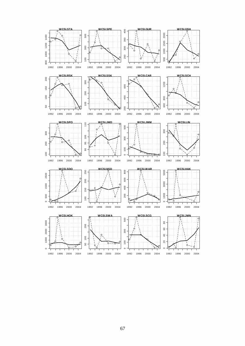
19

For YCS analyses, the monthly range of the environmental predictor within each year was restricted to a period reflecting the Main Spawn Season, as listed in Table 3. The year class strength (YCS) indices were also adjusted (offset) so that the year corresponded to the birth year, after assuming the spawning seasons given in Table 3. This required that the trawl surveys were allocated to a nominal month (Table 4). For some trawl surveys, YCS was available for two adjacent age groups of the same species. These were not combined to obtain a single YCS. It should be noted, however, that the biomass estimates for the same cohort in subsequent years were not always highly correlated. This perhaps emphasises the uncertainty in some of the data (Figure 1).

0 10 20 30 40 50 600

50

100

150

200

88

89

97

98

99

0001

HAK

0 50 100 150 200 2500

200

400

600

800

88

89

97

9899

0001

LIN

Number of fish (’000) at age 3

Num

ber

of fi

sh (

’000

) at

age

4

Figure 1: Comparison of pairs estimates of year-class biomass for HAK and LIN in trawl survey series SubA (the plotting symbol is the last two digits of the birth year of the year class). There were also cases where the YCS for a species was highly correlated between two adjacent areas, notably for GUR and SWA between the WCSI and Tasman Bay (TB) (Table 5). These were treated as separate indices, and not combined into a single index. Table 5: Correlations between YCS indices for the same species in different area. First series Second series Correlation Years in common HAK1235689 HAK4 0.41 29 SKI1+9 SKI7+8 -0.02 16 GUR9 GUR1 -0.10 11 HAK1235689 HAK5+6 0.29 11 HAK4 HAK5+6 -0.32 11 BAR7WC BAR7TB 0.28 10 RCO3-6 RCO7 -0.40 8 SNA1 SNA8+9 -0.39 8 GUR7WC GUR7TB 0.83 7 SWA7WC SWA7TB 0.92 7 RCO7WC RCO7TB 0.19 7 HAK1235689 HAK7WC -0.43 6 HAK4 HAK7WC -0.16 6 GUR9 GUR9tr 0.54 5 GUR1 GUR9tr -0.57 5 The first step in the analyses was predictor screening (Francis 2006), where environmental predictors were removed from the analysis set if they were unlikely to be related to the predictand, because of the area they were associated with. Predictor screening was subjective,

20

and not based on the data or results. For example, the ZN index, of the strength of westerlies over the North Island, would not be expected to be related to YCS or biomass of species found in the subantarctic. The Trenberth and SOI predictors included for each area are shown in Table 6. The chlorophyll indices were available only for YCS and biomass indices in the three areas, Chatham Rise, WCSI, and subantarctic. The SST and SSH were available as gridded files, therefore to select appropriate data for each series only the grid points which feed into defined polygons were used. These polygon areas were matched to the surveys or FMAs (Figure 2). The polygon used for each series is given in Table 4, and the areas shown in Figure 3. Table 6: The area-specific environmental indices (predictors) and the Fisheries Management Area (FMA) and trawl survey area to which they were applied. Environmental index FMA Survey Area Z1 : Auckland -Christchurch 1,2,3,4,7,8,9 Chat, TB, WCSI Z2 : Christchurch-Campbell 3,4,5,6,7 Chat, WCSI, SubA Z3 : Auckland-Invercargill 1-9 Chat, TB, WCSI, SubA Z4 : Raoul-Chatham 1,2,3,4,7,8,9 Chat, TB, WCSI M1 : Hobart-Chatham 1,2,3,4,7,8,9 Chat, TB, WCSI M2 : Hokitika-Chatham 2,3,4 Chat M3 : Hobart-Hokitika 7,8,9 TB MZ1 : Gisborne-Hokitika 3,4,7 Chat, WCSI, TB MZ2 : Gisborne-Invercargill 3,5,6,7 WCSI,SubA MZ3 : New Plymouth-Chatham 2,3,4,7,8 Chat,WCSI, TB MZ4 : Auckland-New Plymouth 1,2,8,9 none ZN : Auckland-Kelburn 1,2,8,9 TB ZS : Kelburn-Invercargill 3,4,5,6,7 Chat, WCSI, TB, SubA

Figure 2: New Zealand Fisheries Management Areas (FMA) boundaries and labels. Reproduced from the MFish website (www.fish.govt.nz)

21

165°E 170° 175° 180° 175°

50°S

45°

40°

35°

x x x x x x x x x x x x x x x x x x x x x x xx x x x x x x x x x x x x x x x x x x x x x xx x x x x x x x x x x x x x x x x x x x x x xx x x x x x x x x x x x x x x x x x x x x x xx x x x x x x x x x x x x x x x x x x x x x xx x x x x x x x x x x x x x x x x x x x x x xx x x x x x x x x x x x x x x x x x x x x x xx x x x x x x x x x x x x x x x x x x x x x xx x x x x x x x x x x x x x x x x xx x x x x x x x x x x x x x x x xx x x x x x x x x x x x x x x xx x x x x x x x x x x x x x x xx x x x x x x x x x x x x x x x xx x x x x x x x x x x x x x x x x xx x x x x x x x x x x x x x x x x xx x x x x x x x x x x x x x x x x xx x x x x x x x x x x x x x x x x xx x x x x x x x x x x x x x x x x xx x x x x x x x x x x x x x x x x x x x x x xx x x x x x x x x x x x x x x x x x x x x x xx x x x x x x x x x x x x x x x x x x x x x xx x x x x x x x x x x x x x x x x x x x x x xx x x x x x x x x x x x x x x x x x x x x x x

165°E 170° 175° 180° 175°

50°S

45°

40°

35°

x x x x x x x x x x x x x x x x x x x x x x xx x x x x x x x x x x x x x x x x x x x x x xx x x x x x x x x x x x x x x x x x x x x x xx x x x x x x x x x x x x x x x x x x x x x xx x x x x x x x x x x x x x x x x x x x x x xx x x x x x x x x x x x x x x x x x x x x x xx x x x x x x x x x x x x x x x x x x x x x xx x x x x x x x x x x x x x x x x x x x x x xx x x x x x x x x x x x x x x x x xx x x x x x x x x x x x x x x x xx x x x x x x x x x x x x x x xx x x x x x x x x x x x x x x xx x x x x x x x x x x x x x x x xx x x x x x x x x x x x x x x x x xx x x x x x x x x x x x x x x x x xx x x x x x x x x x x x x x x x x xx x x x x x x x x x x x x x x x x xx x x x x x x x x x x x x x x x x xx x x x x x x x x x x x x x x x x x x x x x xx x x x x x x x x x x x x x x x x x x x x x xx x x x x x x x x x x x x x x x x x x x x x xx x x x x x x x x x x x x x x x x x x x x x xx x x x x x x x x x x x x x x x x x x x x x x

Figure 3: The SST (. and x) and SSH (x only) grid positions and data selection polygons. In the left panel, the polygons shown are, clockwise from bottom, SubA, WCSI, TB and CR. In the right panel, the polygons shown are, clockwise from bottom, FMA56, FMA5, FMA7WCSI, FMA7TB, FMA8, FMA9, FMA1, FMA2, FMA4, FMA3. 2.3.2 Statistical tests In all statistical tests, the data (e.g., predictor and predictand) were restricted to the years that they had in common, and the test was not performed if this overlap was less than 5 years. Two tests for association between the predictors and predictand were performed. First, the environmental predictors were tested for a significant correlation with the predictand. This used Spearman’s rank correlation, as a 2-sided test (so the correlation could be either positive or negative). The test was assumed to be significant at the 5% level. Second, a test of the association of the extremes of the predictor and predictand occurring together was performed. Each predictor and predictand was allocated into a bin: a low bin (L) for the values in the lower quantile, a high bin (H) for values in the upper quantile, and a medium bin (M) for the remainder. The probability that the H values occurred all in H-H pairs, or alternatively all in H-L pairs, was then tested. The null hypothesis was that the pairing of predictor and predictand occurred at random, and the probability calculated was the p-value for a test of this null hypothesis. Based on combinatorial arguments (Appendix C), the probability is:

p =

N i j m n i jN m n m i

N N mm n

− − + − −⎛ ⎞⎛ ⎞⎜ ⎟⎜ ⎟− − −⎝ ⎠⎝ ⎠

−⎛ ⎞⎛ ⎞⎜ ⎟⎜ ⎟⎝ ⎠⎝ ⎠

where !( )! !

N nk n k k

⎛ ⎞=⎜ ⎟ −⎝ ⎠

22

For example, in a series with 20 pairs of observations, 3 would be expected to be in the H bin and 3 in the L bin, leaving 14 in the M bin. If only 1 H-H pairing was in the H bin, and none in the low bin, the p-value would be 0.15 and not significant. If there were 2 H-H pairings in the H bin, and 1 L-L pairing in the L bin, the p-value would be 0.002, and significant. The test was assumed to be significant at the 5% level, and in this example, would mean at least 2 pairs (out of the possible 6) would have to be in the correct bins. For a shorter data series, for example with 7 pairs, the test would expect 1 H-H pair and 1 L-L pair, and both would have to be correctly associated for the p-value to be significant. The test was assumed to be significant at the 5% level. A significant result would therefore indicate that the extremes were paired together more often than would occur by chance. If the pairing was H-H, then the relationship was considered positive, if the pairing was H-L, the relationship was negative. A final test used in the analyses was for time series (YCS or biomass) moving together. The null hypothesis for this test is that the series were unrelated, against the alternative that they were correlated with one another. The test calculated ranks for the observations in each series (riy: i = 1,...,nseries; y = 1,...,nyear), and then mean ranks across all series (ry = meani(riy)) (Table 7). Table 7: An example of the allocation of YCS to ranks, and mean rank, for YCS indices from Tasman Bay. Year of birth Series 1990 1992 1993 1995 1998 2001 2003 YCSs SWA7TB 3.559 0.511 0.334 1.514 0.826 0.197 0.059 GUR7TB 1.253 0.504 0.978 1.987 1.666 0.076 0.535 RCO7TB 0.703 0.138 0.733 4.567 0.036 0.078 0.745 TAR7TB 2.417 0.593 1.710 1.026 0.593 0.616 0.046 BAR7TB 0.171 7.277 0.37 0.882 0.104 0.389 0.028 Ranks, riy SWA7TB 7 4 3 6 5 2 1 GUR7TB 5 2 4 7 6 1 3 RCO7TB 4 3 5 7 1 2 6 TAR7TB 7 2.5 6 5 2.5 4 1 BAR7TB 3 7 4 6 2 5 1 Mean ranks, ry 5.2 3.7 4.4 6.2 3.3 2.8 2.4 The closeness statistic, s0, indicates how closely the series are correlated with one another, and is estimated as:

( )0

0.52

,mean i y iy ys r r= ⎡ ⎤−⎢ ⎥⎣ ⎦

Low values of s0 suggest that the series fluctuate synchronously. In order to see whether s0 is small enough to reject the null hypothesis, the data were then replaced by random numbers (drawn from a uniform distribution), and the above calculation repeated to generate a new closeness statistic, s1. This was done 1000 times, with 1000 different sets of random numbers, generating 1000 closeness statistics. The proportion of these randomly generated closeness statistics that were less than or equal to s0 was taken as a p-value in our hypothesis test. The test was assumed to be significant at the 5% level. As an example, the test applied to the data in the example above returned an (only just) significant result of common years = 7; p-value = 0.048. It is worth noting that when applied to a single pair of indices, this approach gives similar p-values to the Spearman rank correlation test. The Spearman rank correlation test was therefore used in pairwise analyses for simplicity.

23

3. RESULTS 3.1 Fisheries and climate correlations The data set included 44 YCS and 168 biomass indices, and 253 significant rank correlations were found (Table 8). It is interesting to note that 79 additional significant rank correlations were excluded because the combination of predictor and predictand was screened (these are not shown in Table 8). The occurrence of 79 significant results for combinations highly unlikely to be true highlights the substantial potential for spurious correlations, and the importance of predictor screening. Significant rank correlations were detected for 21 of the 48 YCS series (44%) and 86 of the 172 biomass series (50%). The significant rank correlations were most frequently with SST (N=43), SSH (N=28), Trough (N=26), Blocking (N=23) and SOI (N=22), followed by Z4 (N=16: Westerly winds over 30–45° S), M3 (N=13, Southerly winds over the Tasman Sea), and Zonal (N=13). 3.2 Short-lived species The only species identified as having a short life span was arrow squid (see Table 3). On the WCSI, the assumed YCS had a significant negative correlation with SST, and a significant association with MZ4. However, this result is likely to be spurious, because the YCS index for the WCSI actually indexes an unknown mix of two different species, the southern species Nototodarus sloanii and northern species N. gouldi. Uozomi (1998) found N. gouldi was the dominant species at the southern edge of the North Island, on the west coast of the South Island the species mix was about 50:50, and in the subantarctic the only species was N. sloanii. Because the separate species were not identified in trawl surveys, the species mix in the YCS and biomass indices (both derived from research trawl survey catch rates) was unclear, and could not be interpreted. But as low YCS was associated with high temperature we might hypothesise that the species being measured may have been predominantly the southern species, N. sloanii. Table 8: Summary of the results of the rank correlation and association tests for each data series. The ‘series’ and ‘type’ describe the species, area, where relevant the age class, and the type of index (YCS, year class strength; TRAWl or CPUE, biomass; see Table 3). The ‘rank correlation’ and association test columns list the environmental or climate indices which were significant at the 5% level in the rank correlation or association tests. “–“ indicates no significant results.

Common name Series Type Rank correlation Association test

Arrow squid TBGB.ASQ TRAWL YCS - - WCSI.ASQ TRAWL YCS SST - TBGB.ASQ TRAWL - - WCSI.ASQ TRAWL Trough -

Barracouta BAR7TB YCS (0+) - M1, M3, ZS, SOI, Trough, Zonal, Blocking, SST

BAR7WC YCS (1+) - M2, ZS, MZ1, Trough, Zonal BAR1.WCSI YCS - - BAR2.WCSI YCS MZ1, Trough, Zonal MZ1, Trough, Zonal BAR0.TB YCS Zonal - BAR1.TB YCS - - FMA8.BAR TRAWL - - FMA9.BAR TRAWL - - TBGB.BAR TRAWL - - WCSI.BAR TRAWL - - BAR1 CPUE - Z2, M3, ZS, MZ2, Trough,

Zonal

24

Table 7 (cont.) Common name Series Type Rank correlation Association test

BAR5 CPUE Trough -

Banded bellowsfish

Chat.BBE TRAWL SSH Z1, Z2, Z3, Z4, M1, M2, ZS, MZ1, SOI, Zonal, SSH

Blue cod TBGB.BCO TRAWL - - BCO5 CPUE SOI, Trough, Blocking,

SSH SOI, Trough, Blocking, SST, SSH

Carpet shark TBGB.CAR TRAWL Z1, Z4, ZN, MZ3, Trough, Blocking, SST

-

WCSI.CAR TRAWL Z4, Blocking, SST -

Oblique banded rattail

Chat.CAS TRAWL Z1, Trough, SSH Z1, Z2, Z4, M1, M2, MZ1, SOI, Trough, Zonal, Blocking, SST, SSH

SubA.CAS TRAWL - ZS, MZ2, SOI

Two saddle rattail Chat.CBI TRAWL M2, MZ3 Z1, Z2, Z4, M1, M2, ZS, MZ1, MZ3, SOI, Trough, Zonal, Blocking

Bollon’s rattail Chat.CBO TRAWL Z3 Z2, Z3, Trough, Zonal, SST, SSH

Banded rattail Chat.CFA TRAWL - Z1, Z3, Z4, M1, M2, MZ3, SOI, Trough, Zonal, SSH

SubA.CFA TRAWL Trough, Zonal, Blocking Trough, Blocking, SST

Oliver’s rattail Chat.COL TRAWL ZS Z1, Z2, Z4, M2, MZ1, SOI, Zonal, Blocking, SST, SSH

SubA.COL TRAWL Z2, mean, anom Trough, mean, anom

Cucumber fish WCSI.CUC TRAWL - -

Elephantfish WCSI.ELE TRAWL MZ1 - ELE3 CPUE SOI, Blocking, SST,

SSH Z1, Z2, Z4, M1, M2, ZS, MZ1, MZ2, MZ3, SOI, Trough, Zonal, Blocking, SST, SSH

ELE5 CPUE - Z3, ZS, MZ2, SOI, Blocking

Electric ray TBGB.ERA TRAWL - - WCSI.ERA TRAWL - Z4, M1, ZS, MZ3, SOI, Trough,

SST N.Z. sole TBGB.ESO TRAWL - ZN WCSI.ESO TRAWL Z4, M1, M3, ZN, MZ3,

SOI, Trough, Blocking, SST

Z4, M1, ZS, MZ3, SOI, Trough, SST

Deepsea flathead Chat.FHD TRAWL - Z2, ZS, MZ1, MZ3, SOI, Trough, Zonal, Blocking, SST, SSH

Frostfish WCSI.FRO TRAWL Z4, M3, MZ3, Trough, Blocking, SST

M3, ZS, Blocking

Grey mullet GMU1 CPUE Z3 Z3, MZ4, Trough

Ghost shark Chat.GSH TRAWL SST, SSH Z1, M2, MZ1, MZ2, SOI, Zonal, SST, SSH

SubA.GSH TRAWL - Z4, SOI WCSI.GSH TRAWL Zonal Z4, M1, ZS, MZ3, SOI, Trough,

SST Pale ghost shark Chat.GSP TRAWL - Z2, Z4, M1, M2, ZS, MZ1,

MZ4, Zonal, mean, anom, SST, SSH

SubA.GSP TRAWL Trough Trough

Red gurnard GUR1 YCS - Z1, Z3, M1, ZN, MZ3, MZ4, SOI, Trough, Blocking

GUR7TB YCS M1 - GUR7WC YCS M1, M3, SOI M1, MZ2, SOI, SST, SSH GUR9 YCS - Z3, MZ4, Trough, Zonal BoP.GUR TRAWL - - FMA8.GUR TRAWL - -

25


FMA9.GUR TRAWL Z1, Z3, Z4, M1, ZN, SOI, Blocking, SST

Z1, Z4, M1, ZN, Blocking, SST

HG.GUR TRAWL - - TBGB.GUR TRAWL - - WCSI.GUR TRAWL - - GUR1 CPUE - M1 GUR2 CPUE Z4, MZ4, SOI, Trough,

Zonal, SSH Z1, Z4, M1, MZ3, SOI, Trough, Blocking, SST, SSH

GUR3 CPUE - Z3, ZS, MZ2, Trough, Zonal

Hake HAK1235689 YCS - Z2, Z3, MZ2, Zonal, Blocking, SST

HAK4 YCS SOI, Trough, Blocking, SSH

Z1, Z2, Z3, Z4, M1, M2, MZ1, MZ2, MZ3, SOI, Trough, Zonal, Blocking, SST

HAK5+6 YCS - Z2, Zonal, mean, anom, SST HAK7WC YCS MZ3 - HAK3.SubA YCS (3+) Z2, Z3, MZ2, SST Z2, Z3, Zonal, mean, anom HAK4.SubA YCS (4+) - mean anom Chat.HAK3 YCS (3+) Z2, Trough Z1, Z2, Z3, Z4, M1, M2,

Trough, Zonal, Blocking, mean, anom

Chat.HAK4 YCS (4+) Trough Z1, Z2, Z3, Z4, M1, M2, ZS, MZ1, MZ3, SOI, Trough, Zonal, Blocking, SST

Chat.HAK TRAWL SST, SSH Z2, ZS, MZ1, MZ3, SOI, Trough, Zonal, Blocking, SST, SSH

Chat.HAK3 TRAWL SSH Z1, Z3, SOI, Blocking, SST, SSH

Chat.HAK4 TRAWL - Z1, Z3, M1, M2, ZS SubA.HAK TRAWL - - SubA.HAKa TRAWL - - WCSI.HAK TRAWL - - HAK1 CPUE M3, MZ4, Trough,

Blocking, SST, SSH Z1, Z4, M1, M3, ZN, ZS, MZ1, MZ3, MZ4, SOI, Trough, Blocking, SST, SSH

HAK4cpue CPUE Trough, SSH Z1, Z2, Z3, Z4, M1, ZS, MZ1, MZ3, SOI, Trough, Zonal, Blocking, SST, SSH

Hapuku WCSI.HAP TRAWL Z4, M1, M3, Trough, Zonal, SST

Zonal

Hoki HOKe YCS (0) - Z1, Z2, Z3, Z4, M1, M2, ZS, MZ1, MZ3, SOI, Zonal, Blocking, SST, SSH

HOKw YCS (0) SST Z1, Z2, Z3, Z4, M1, M3, ZS, MZ1, MZ2, MZ3, SOI, Trough, Zonal, Blocking, SST

HOK.chat YCS (1+) Z4, M1, SOI, Blocking, SST

Z1, Z2, Z3, Z4, M1, M2, ZS, MZ3, SOI, Trough, Zonal, Blocking, SST, SSH

Chat.HOK TRAWL ZS, SST, SSH Z2, Z3, M2, ZS, SOI, Blocking, SST, SSH

SubA.HOK TRAWL - Z3, ZS, MZ2, SOI WCSI.HOK TRAWL - -

Javelinfish Chat.JAV TRAWL SST, SSH Z1, Z2, Z3, MZ1, SOI, Blocking, SST, SSH

SubA.JAV TRAWL - Trough

John dory JDO9 YCS - - BoP.JDO TRAWL - Z4, M1, M2 BoP.JDO1 TRAWL - Z3

26


FMA8.JDO TRAWL - - FMA9.JDO TRAWL Zonal - HG.JDO TRAWL - Z3 TBGB.JDO TRAWL - - WCSI.JDO TRAWL MZ1 -

Jack mackerel (declivis)

TBGB.JMD TRAWL Zonal Z4, M1, ZS, MZ3, SOI, Trough

WCSI.JMD TRAWL Zonal -

Jack mackerel (murphyi)

WCSI.JMM TRAWL Z4, Blocking, SST -

Jack mackerel (novaezelandiae)

TBGB.JMN TRAWL Z3 Zonal

WCSI.JMN TRAWL - -

Lookdown dory Chat.LDO TRAWL SOI, SST Z1, Z2, Z4, ZS, MZ1, SOI, Blocking, SST, SSH

SubA.LDO TRAWL ZS, SST Blocking, SST

Leatherjacket BoP.LEA TRAWL Trough Z4, M1 HG.LEA TRAWL - Z1, Trough TBGB.LEA TRAWL Zonal - WCSI.LEA TRAWL - -

Ling LIN5+6 YCS (3+) Zonal Z2, Z3, ZS, MZ2, Trough, SST LIN34 YCS (0) - Z1, Z2, Z3, Z4, M1, M2, ZS,

MZ1, MZ2, MZ3, SOI, Trough, Zonal, Blocking, SST, SSH

LIN56 YCS (0) - Z2, Z3, ZS, MZ2, SOI, Trough, Zonal, Blocking, SST, SSH

LIN7WC YCS (0) M1, M3, SOI, SST, SSH Z1, Z2, Z3, Z4, M1, M3, ZS, MZ1, MZ2, MZ3, SOI, Zonal, Blocking, SST, SSH

LIN3.SubA YCS (3+) - Z2, Zonal LIN4.SubA YCS (4+) - - Chat.LIN3 YCS (3+) - Z1, Z3, M2, ZS, MZ1, MZ3,

Trough, Zonal, mean, anom, SST

Chat.LIN4 YCS (4+) - Z1, Z3, Z4, M1, M2, ZN, ZS, MZ1, MZ3, SOI, Zonal, SSH

Chat.LIN TRAWL - Z1, Z2, Z4, MZ3, Trough, Zonal, locking, SST, SSH

Chat.LIN3 TRAWL SST, SSH Z1, Z2, Z4, M1, M2, MZ1, MZ3, SOI, Blocking, SST, SSH

Chat.LIN4 TRAWL SOI, SST, SSH Z1, Z2, Z4, M1, M2, ZS, MZ1, MZ3, SOI, Trough, Zonal, Blocking, SST, SSH

SubA.LIN TRAWL - Trough WCSI.LIN TRAWL Z1 - LIN1 CPUE M1, SOI, SST Z3, M3, ZN, MZ4, SOI, Trough,

Zonal, Blocking, SST LIN2 CPUE SOI, Blocking, SSH Z1, Z3, Z4, M1, M2, ZN, MZ3,

MZ4, SOI, Trough, Zonal, Blocking

LIN3&4 CPUE SST, SSH Z3, Z4, M1, ZS, MZ3, SOI, Trough, Blocking, SST, SSH

LIN5&6 CPUE - Z3, ZS, MZ2, SOI, Trough, Blocking, SST, SSH

LIN6 CPUE - Z2, Z3, ZS, Blocking, SST, SSH LIN7 CPUE ZS, SST, SSH Z2, Z3, ZS, MZ1, MZ2, SOI,

SST, SSH Lemon sole TBGB.LSO TRAWL MZ1 - WCSI.LSO TRAWL Z4, Trough, Blocking,

SST -

27


Northern spiny dogfish

WCSI.NSD TRAWL - -

Rubyfish RBY2 CPUE MZ4, Trough -

Red cod RCO3-6 YCS - Z1, Z2, Z3, MZ2, Trough, Zonal RCO7 YCS - Zonal RCO7TB YCS - - RCO7WC YCS Blocking SOI TBGB.RCO TRAWL YCS SST SST WCSI.RCO TRAWL YCS SST Trough RCO3 CPUE YCS - Z1, Z3, MZ2, SST, SSH RCO7cpue CPUE YCS Z1, Z3, ZS, MZ2 Z1, Z3, MZ2, MZ3, SST TBGB.RCO TRAWL - - WCSI.RCO TRAWL Z1, Z4, Trough,

Blocking, SST Z1

RCO3 CPUE M2 M2, MZ1, MZ3, SSH RCO7 CPUE - Z2

Ribaldo Chat.RIB TRAWL Z3, mean, anom Z1, Z2, Z3, Z4, M1, ZS, MZ1, mean, anom, SST

SubA.RIB TRAWL - -

Rough skate TBGB.RSK TRAWL Z4, M3, ZN, Trough, Blocking

M3, ZS, SST

WCSI.RSK TRAWL MZ1 -

Southern blue whiting

SubA.SBW TRAWL - SOI

SBW6B CPUE Trough ZS, Trough SBW6I CPUE SOI, SST Z2, SOI, Trough, Zonal,

Blocking Scaly gurnard TBGB.SCG TRAWL - - WCSI.SCG TRAWL MZ1 -

School shark FMA8.SCH TRAWL - - FMA9.SCH TRAWL - - TBGB.SCH TRAWL M1, MZ2, MZ3, SOI,

SST -

WCSI.SCH TRAWL M3 - SCH1 CPUE SOI, SST, SSH Z1, Z3, Z4, M1, M3, SOI, SSH SCH3 CPUE - Z1, ZN, MZ1, MZ2, SOI,

Trough, Zonal, SST, SSH SCH5 CPUE - Z2, Z3, ZS, MZ2, mean, anom,

SST, SSH SCH7 CPUE - Z2, Z4, M1, M3, ZS, MZ2,

MZ3, SOI, Trough, Zonal, SSH SCH8 CPUE M3, Trough, Zonal Z1, Z4, M1, M3, ZN, MZ3,

MZ4, SOI, Trough, Zonal, Blocking, SST, SSH

Silver dory Chat.SDO TRAWL - Z2, Z3, M1, M2, ZS, MZ2, MZ3, Zonal, Blocking, SST

WCSI.SDO TRAWL - -

Sand flounder HG.SFL TRAWL - ZN, Zonal, Blocking TBGB.SFL TRAWL ZN ZN

Gemfish SKI1+9 YCS - Z1, Z3, M1, M3, ZN, MZ4, Trough, Zonal, Blocking, SST

SKI7+8 YCS Z4, SST Z1, Z4, M1, M3, ZN, ZS, MZ1, MZ3, MZ4, Trough, Zonal, Blocking, SST

WCSI.SKI TRAWL Z3, MZ2 - SKI1 CPUE SSH Z1, Z3, Z4, ZN, MZ4, SOI,

Trough, Zonal, SST SKI2 CPUE - Z1, Z3, Z4, M1, M2, ZN, MZ2,

MZ3, Trough, Zonal, Blocking

28


Snapper SNA1 YCS SOI, SST Z3, Z4, M1, M2, ZN, MZ4, SOI, Trough, Blocking

SNA8+9 YCS - Z4, MZ3, Zonal SNA9 YCS - Z1, ZN BoP.SNA TRAWL - Z1,SOI, Blocking BoP.SNA2 TRAWL - - FMA8.SNA TRAWL - - FMA9.SNA TRAWL - - HG.SNA TRAWL Zonal, Blocking, SST ZN SNA1cpue CPUE Z4, M1, SOI, Blocking,

SST Z1, Z3, Z4, M1, M2, ZN, MZ4, SOI, Blocking, SST

Shovelnose dogfish

Chat.SND TRAWL - Z1, Z2, Z3, Z4, M1, M2, ZS, MZ1, SOI, Trough, Zonal, mean, anom, SST, SSH

Spiny dogfish FMA8.SPD TRAWL - - FMA9.SPD TRAWL - - SubA.SPD TRAWL - Z3, ZS, MZ1, MZ2, SOI TBGB.SPD TRAWL - - WCSI.SPD TRAWL MZ1 Z2, MZ1, MZ2 Chat.SPD TRAWL SOI, SST, SSH Z2, Z3, Z4, M2, ZS, MZ1, SOI,

Blocking, SST, SSH SPD3 CPUE MZ3 Z1, M1, ZN, SSH SPD5 CPUE - Z3 SPD6 CPUE - Z2, Zonal, SSH SPD7 CPUE SSH SOI, Zonal, SST, SSH

Sea perch Chat.SPE TRAWL SST, SSH Z2, Z3, M2, MZ1, Blocking, SSH

TBGB.SPE TRAWL - - WCSI.SPE TRAWL MZ1 - SPE3 CPUE M2, SST M2, MZ3

Rig FMA8.SPO TRAWL - - FMA9.SPO TRAWL - SOI TBGB.SPO TRAWL - - WCSI.SPO TRAWL - - SPO3 CPUE - Z1, Z2, Z3, ZN, MZ3, Blocking SPO7 CPUE - Z1, Z2, ZN, MZ1, SST SPO8 CPUE - Z1, Z3, ZN, MZ4, SOI, SST,

SSH Smooth skate WCSI.SSK TRAWL Z4, Trough, Blocking,

SST -

Stargazer TBGB.STA TRAWL Z1 Z1 WCSI.STA TRAWL - - STA3 CPUE Z1, Z3 Z1, Z2, Z3, Z4, M2, ZN, MZ1,

MZ2, MZ3, SOI, Trough, Zonal, Blocking

STA4 CPUE - - STA5 CPUE - Z3, ZS, MZ2, SOI, Zonal, mean,

anom STA7 CPUE M1, M3, SOI, Blocking,

SST, SSH Z1, Z4, M1, M3, ZS, MZ1, MZ2, MZ3, SOI, Trough, Blocking, SST, SSH

Silver warehou SWA7TB YCS - - SWA7WC YCS M2 - TBGB.SWA TRAWL - Zonal WCSI.SWA TRAWL Z3, MZ1, MZ2 Z2, MZ1, MZ2

Tarakihi TAR7TB YCS - - TBGB.TAR TRAWL M3 - WCSI.TAR TRAWL - -

29


TAR1 CPUE - MZ4, SSH TAR2 CPUE SOI, SST, SSH Z1, Z4, ZN, SOI, Blocking, SST TAR3 CPUE - Z1, Z4, M1, M2, ZN, ZS, MZ3,

SOI, Trough, Blocking, SST, SSH

Trevally FMA8.TRE TRAWL - - FMA9.TRE TRAWL - - TRE7 CPUE MZ4, Trough Z1, Z2, Z3, Z4, M1, M3, ZN,

ZS, MZ2, MZ3, MZ4, SOI, Trough, Zonal, Blocking, SST, SSH

Common warehou TBGB.WAR TRAWL - - WCSI.WAR TRAWL Z1, Z3 Z3

Witch TBGB.WIT TRAWL Z4, M3, ZN, Trough, Blocking

M3, ZS, Blocking, SST

WCSI.WIT TRAWL - -

White warehou SubA.WWA TRAWL Z3, MZ2 -

3.3 Cold water species 3.3.1 Common trends in YCS and biomass of cold water species There was no significant common trend in YCS indices when adjusted to the birth year, for the following species datasets: WCSI (HOKw & species with -1 year offset, N=3, common years=5, p=0.61; HOKw & species with -2 year offset, N=5, common years=7, p=0.15), or the Chatham Rise (HAK4 & HOKw, N=2, common years=26, p=0.53; Chat.HAK3 & HOK.Chat, N=2, common years=13, p=0.09). The only YCS indices available for the subantarctic were for hake. The biomass indices from the Chatham Rise trawl survey did not show any common trend (N=7, common years=15, p=0.61). Combined with the YCS result, this suggests no common catchability or YCS influence amongst these species on the Chatham Rise. The biomass indices from the WCSI trawl survey showed a significant common trend (N=9, common years=6, p=0.003), with all of the indices except dark ghost shark and silver warehou showing an overall decline between the first half on the index and the second half. When examined in finer detail, however, common patterns were not obvious, except for a similar pattern in red cod and spiny dogfish. For red cod, spiny dogfish, and stargazer biomass indices were also available from WCSI fisheries, but these did not show a common trend (N=3, common years=9, p=0.26). This suggests there may be a common catchability effect amongst cold water species in the WCSI trawl survey. The biomass indices from the subantarctic showed a significant common pattern for the trawl survey (N=10, common years=9, p<0.001), but not for the commercial CPUE indices (N=4, common years= 8, p=0.91). Detailed examination suggested similar biomass patterns in the subantarctic trawl survey between banded rattail, hake, dark ghost shark and pale ghost shark (N=4, common years=9, p<0.001), hoki and oblique banded rattail (N=2, common years=9, p=0.02), and white warehou and spiny dogfish (N=2, common years=9, p=0.04).

30

3.3.2 Relationships with climate for cold water species Six of the 12 cold water species showed correlations with climate indices that could be consistent with increasing recruitment and catchability towards the northern limit of their range when temperatures were lower and southerly winds stronger (Figure 4). Banded rattail biomass on the Chatham Rise had a negative correlation with SSH. Hake YCS on the Chatham Rise, estimated from the stock assessment model, had a negative correlation with SOI and Blocking, and hake biomass a negative correlation with SST and SSH, although the trend was unidirectional. However, the index of 3+ hake from the Chatham Rise trawl survey suggests a recovery in YCS in 2005–06, which correlated with SSH and Trough. Hake YCS in the subantarctic had a weak negative correlation with SSH, but was unclear as the subantarctic time series was short. Barracouta biomass on the WCSI had no correlation with SST or SSH, but a significant positive correlation with the Trough regime suggested catchability was higher in cooler conditions. Hoki YCS from the Chatham Rise trawl survey had a weak negative correlation with SST, Blocking, and SOI, and a weak positive correlation with stronger southerlies and westerlies (M1 and Z4), but the model output YCS had no significant correlation. The negative correlation between hoki biomass and SSH appeared stronger but reflected predominantly one-way trends, with a major fish-down of hoki having taken place during the late 1980s and 1990s. Red cod biomass on the WCSI had a significant positive correlation with the Trough regime, and negative with SST, suggesting catchability was higher in cooler conditions. Silver warehou biomass on the WCSI had a negative correlation with MZ1 and MZ2, implying lower catchability with strong northwesterlies. Six of the 12 southern species showed correlations with climate indices that could be considered inconsistent with increasing recruitment and catchability towards the northern limit of their range when temperatures were lower and southerly winds stronger (Figure 4). Blue cod biomass off Southland had a positive correlation with SSH, SOI, and the Blocking regime, and a negative correlation with Trough, although the biomass trend was unidirectional (it increased). Oblique-banded rattail biomass on the Chatham Rise was positively correlated with SSH, and weakly negatively correlated with Trough, but the biomass index was increasing roughly 1 year ahead of the SSH, which suggests no causal link. Elephantfish biomass on the east coast of the South Island had a strong positive correlation with SST and SSH. Elephant fish biomass off Southland (ELE5) had a similar trend, but there were no significant correlations with climate. Dark ghost shark biomass on the Chatham Rise had a weak positive correlation with SST and SSH, but these were predominantly unidirectional. Stargazer biomass on the WCSI from CPUE (STA7) had a positive correlation with SST and SOI, whereas stargazer biomass (CPUE) off Southland had no clear association with SOI. There was also no significant correlation for stargazer in the WCSI trawl survey (WCSI.STA), which was also inconsistent with the fishery index. Spiny dogfish biomass on the Chatham Rise had a significant positive correlation with SST, SSH and SOI. Southern blue whiting is a predominantly southern subantarctic species, and the eastern stock (SBW6B) appeared positively correlated with Trough, with an notable outlier in 1994. White warehou correlations were unclear.

31

600 1000 1400

-3-1

12

3

Chat.CAS

SS

H

Chat.CAS vs. SSH

1992 1996 2000 2004

0.0

0.4

0.8

Year

Inde

x

Chat.CAS vs. SSH

0.5 1.0 1.5 2.0

-3-2

-10

1

HAK4

SO

I

HAK4 vs. SOI

1975 1985 1995

0.0

0.4

0.8

Year

Inde

x

HAK4 vs. SOI

0.5 1.0 1.5 2.0

2030

4050

HAK4

Blo

ckin

g

HAK4 vs. Blocking

1975 1985 1995

0.0

0.4

0.8

Year

Inde

x

HAK4 vs. Blocking

1000 2000 3000 4000

12.0

12.4

12.8

13.2

Chat.HAK

SS

T

Chat.HAK vs. SST

1992 1996 2000 2004

0.0

0.4

0.8

Year

Inde

x

Chat.HAK vs. SST

1000 2000 3000 4000

-3-1

12

3

Chat.HAK

SS

H

Chat.HAK vs. SSH

1992 1996 2000 2004

0.0

0.4

0.8

Year

Inde

x

Chat.HAK vs. SSH

0 50000 150000

-3-1

12

3

Chat.HAK3

SS

H

Chat.HAK3 vs. SSH

1992 1996 2000 2004

0.0

0.4

0.8

Year

Inde

x

Chat.HAK3 vs. SSH

0 50000 150000

2530

3540

4550

Chat.HAK3

Trou

gh

Chat.HAK3 vs. Trough

1995 2000 2005

0.0

0.4

0.8

Year

Inde

x

Chat.HAK3 vs. Trough

0.5 1.0 1.5 2.0 2.5

-4-2

02

4

HAK5+6

SS

H

HAK5+6 vs. SSH

1999 2001 2003 2005

0.0

0.4

0.8

Year

Inde

xHAK5+6 vs. SSH

1500 2500 3500

3540

4550

WCSI.BAR

Trou

gh

W CSI.BAR vs. Trough

1992 1996 2000 2004

0.0

0.4

0.8

Year

Inde

x

W CSI.BAR vs. Trough

0 50000 150000

10.5

11.0

11.5

12.0

HOK.chat

SS

T

HOK.chat vs. SST

1995 2000 2005

0.0

0.4

0.8

Year

Inde

x

HOK.chat vs. SST

0 50000 150000

2530

35

HOK.chat

Blo

ckin

g

HOK.chat vs. Blocking

1995 2000 2005

0.0

0.4

0.8

Year

Inde

x

HOK.chat vs. Blocking

0 50000 150000

-1.5

-0.5

0.5

HOK.chat

SO

I

HOK.chat vs. SOI

1995 2000 2005

0.0

0.4

0.8

Year

Inde

x

HOK.chat vs. SOI

Figure 4: Relationships between fisheries and climate indices for cold water species. Each correlation has two panels; the left panel is an x-y plot of the indices, the right panel is a time-series plot of the fisheries index (solid line) and climate index (broken line) on a common scale (between zero and 1).

32

0 50000 150000

-20

020

40

HOK.chat

M1

HOK.chat vs. M1

1995 2000 2005

0.0

0.4

0.8

Year

Inde

x

HOK.chat vs. M1

0 50000 150000

-10

010

2030

HOK.chat

Z4

HOK.chat vs. Z4

1995 2000 2005

0.0

0.4

0.8

Year

Inde

x

HOK.chat vs. Z4

0.5 1.0 1.5 2.0

10.5

11.0

11.5

12.0

HOKe

SS

T

HOKe vs. SST

1975 1985 1995 2005

0.0

0.4

0.8

Year

Inde

x

HOKe vs. SST

0.5 1.0 1.5 2.0

-30

-10

1030

HOKe

M1

HOKe vs. M1

1975 1985 1995 2005

0.0

0.4

0.8

Year

Inde

x

HOKe vs. M1

60000 120000 180000

-3-1

12

3

Chat.HOK

SS

H

Chat.HOK vs. SSH

1992 1996 2000 2004

0.0

0.4

0.8

Year

Inde

x

Chat.HOK vs. SSH

500 1500 2500

3540

4550

WCSI.RCO

Trou

gh

W CSI.RCO vs. Trough

1992 1996 2000 2004

0.0

0.4

0.8

Year

Inde

x

W CSI.RCO vs. Trough

500 1500 2500

14.0

14.5

15.0

15.5

WCSI.RCO

SS

T

W CSI.RCO vs. SST

1992 1996 2000 2004

0.0

0.4

0.8

Year

Inde

x

W CSI.RCO vs. SST

50 100 200

-10

-50

5

WCSI.SWA

MZ1

W CSI.SW A vs. MZ1

1992 1996 2000 2004

0.0

0.4

0.8

Year

Inde

x

W CSI.SW A vs. MZ1

50 100 200

-10

-50

5

WCSI.SWA

MZ2

W CSI.SW A vs. MZ2

1992 1996 2000 2004

0.0

0.4

0.8

Year

Inde

x

W CSI.SW A vs. MZ2

1.1 1.3 1.5

-4-2

02

4

BCO5

SS

H

BCO5 vs. SSH

1992 1996 2000

0.0

0.4

0.8

Year

Inde

x

BCO5 vs. SSH

1.0 1.2 1.4 1.6

-1.0

-0.5

0.0

0.5

BCO5

SO

I

BCO5 vs. SOI

1990 1994 1998

0.0

0.4

0.8

Year

Inde

x

BCO5 vs. SOI

1.0 1.2 1.4 1.6

3035

4045

BCO5

Blo

ckin

g

BCO5 vs. Blocking

1990 1994 1998

0.0

0.4

0.8

Year

Inde

x

BCO5 vs. Blocking

Figure 4 (cont.): Relationships between fisheries and climate indices for cold water species. Each correlation has two panels; the left panel is an x-y plot of the indices, the right panel is a time-series plot of the fisheries index (solid line) and climate index (broken line) on a common scale (between zero and 1).

33

1.0 1.2 1.4 1.6

2530

3540

4550

BCO5

Trou

gh

BCO5 vs. Trough

1990 1994 1998

0.0

0.4

0.8

Year

Inde

x

BCO5 vs. Trough

600 1000 1400

-3-1

12

3

Chat.CAS

SS

H

Chat.CAS vs. SSH

1992 1996 2000 2004

0.0

0.4

0.8

Year

Inde

x

Chat.CAS vs. SSH

600 1000 1400

2530

3540

4550

Chat.CAS

Trou

gh

Chat.CAS vs. Trough

1992 1996 2000 2004

0.0

0.4

0.8

Year

Inde

x

Chat.CAS vs. Trough

0.6 1.0 1.4 1.8

11.5

12.0

12.5

ELE3

SS

T

ELE3 vs. SST

1990 1995 2000 2005

0.0

0.4

0.8

Year

Inde

x

ELE3 vs. SST

0.8 1.2 1.6

-3-1

12

34

ELE3

SS

H

ELE3 vs. SSH

1992 1996 2000 2004

0.0

0.4

0.8

Year

Inde

x

ELE3 vs. SSH

0.6 1.0 1.4 1.8

-4-2

02

4

ELE5

SS

H

ELE5 vs. SSH

1992 1996 2000 2004

0.0

0.4

0.8

Year

Inde

x

ELE5 vs. SSH

4000 8000 12000

12.0

12.4

12.8

13.2

Chat.GSH

SS

T

Chat.GSH vs. SST

1992 1996 2000 2004

0.0

0.4

0.8

Year

Inde

x

Chat.GSH vs. SST

4000 8000 12000

-3-1

12

3

Chat.GSH

SS

H

Chat.GSH vs. SSH

1992 1996 2000 2004

0.0

0.4

0.8

Year

Inde

xChat.GSH vs. SSH

0.8 1.0 1.2 1.4

14.5

15.5

16.5

STA7

SS

T

STA7 vs. SST

1990 1995 2000 2005

0.0

0.4

0.8

Year

Inde

x

STA7 vs. SST

0.8 1.0 1.2 1.4

-1.0

-0.5

0.0

0.5

STA7

SO

I

STA7 vs. SOI

1990 1995 2000 2005

0.0

0.4

0.8

Year

Inde

x

STA7 vs. SOI

0.9 1.0 1.1 1.2 1.3

-1.0

-0.5

0.0

0.5

STA5

SO

I

STA5 vs. SOI

1990 1994 1998 2002

0.0

0.4

0.8

Year

Inde

x

STA5 vs. SOI

2000 6000 10000

12.0

12.4

12.8

13.2

Chat.SPD

SS

T

Chat.SPD vs. SST

1992 1996 2000 2004

0.0

0.4

0.8

Year

Inde

x

Chat.SPD vs. SST

Figure 4 (cont.): Relationships between fisheries and climate indices for cold water species. Each correlation has two panels; the left panel is an x-y plot of the indices, the right panel is a time-series plot of the fisheries index (solid line) and climate index (broken line) on a common scale (between zero and 1).

34

2000 6000 10000

-3-1

12

3

Chat.SPD

SS

H

Chat.SPD vs. SSH

1992 1996 2000 2004

0.0

0.4

0.8

Year

Inde

x

Chat.SPD vs. SSH

2000 6000 10000

-1.0

-0.5

0.0

0.5

Chat.SPD

SO

I

Chat.SPD vs. SOI

1992 1996 2000 2004

0.0

0.4

0.8

Year

Inde

x

Chat.SPD vs. SOI

0.4 0.6 0.8 1.0 1.2

2530

3540

4550

SBW6B

Trou

gh

SBW 6B vs. Trough

1990 1994 1998 2002

0.0

0.4

0.8

Year

Inde

x

SBW 6B vs. Trough

Figure 4 (cont.): Relationships between fisheries and climate indices for cold water species. Each correlation has two panels; the left panel is an x-y plot of the indices, the right panel is a time-series plot of the fisheries index (solid line) and climate index (broken line) on a common scale (between zero and 1). 3.4 Warm water species 3.4.1 Common trends in YCS and biomass for warm water species YCS indices were available only for snapper, and so no comparisons with other species could be made. Overall, there was no significant common trend in biomass indices for the WCSI (N=8, common years=6, p=0.74), and only limited comparisons could be made around the North Island because of the lack of common years, but where they could be compared these also had no common trends (N=4, common years=5, p=0.75). This suggests no common catchability influence amongst the warm water species. 3.4.2 Relationships with climate for warm water species Two of the 11 northern species (snapper and frostfish) showed correlations with climate indices that could be consistent with increasing recruitment and catchability towards the southern limit of their range when temperatures were higher and northerly winds stronger (Figure 5). For snapper in the East Northland, Hauraki Gulf, and Bay of Plenty stock (SNA1), the positive correlation between YCS and SST has been previously reported, and was found here (it is the same data set) along with a positive correlation with SOI. No similar correlations were found for any other snapper stock. The plot of YCS for SNA 1 and SOI suggests a possibly non-linear (asymptotic) relationship. Snapper biomass for SNA 1 also had a positive correlation with SST, although this was weak. Frostfish biomass on the WCSI was negatively correlated with increased southerlies (M3), and positively correlated with Blocking; this is consistent with higher catchability with decreased southerlies and increased temperature. Indices were not available for frostfish from any other areas.

35

2 4 6 8 10

18.5

19.0

19.5

20.0

SNA1

SS

T

SNA1 vs. SST

1985 1990 1995

0.0

0.4

0.8

Year

Inde

x

SNA1 vs. SST

0.5 1.5 2.5

17.0

17.5

18.0

18.5

SNA8+9

SS

T

SNA8+9 vs. SST

1984 1988 1992 1996

0.0

0.4

0.8

Year

Inde

x

SNA8+9 vs. SST

2 4 6 8 10

-3-2

-10

1

SNA1

SO

I

SNA1 vs. SOI

1985 1990 1995

0.0

0.4

0.8

Year

Inde

x

SNA1 vs. SOI

0.80 0.90 1.00 1.10

17.5

18.0

18.5

19.0

SNA1cpue

SS

T

SNA1cpue vs. SST

1990 1994 1998

0.0

0.4

0.8

Year

Inde

x

SNA1cpue vs. SST

100 300 500

05

1020

WCSI.FRO

M3

W CSI.FRO vs. M3

1992 1996 2000 2004

0.0

0.4

0.8

Year

Inde

x

W CSI.FRO vs. M3

100 300 500

3035

40

WCSI.FRO

Blo

ckin

g

W CSI.FRO vs. Blocking

1992 1996 2000 2004

0.0

0.4

0.8

Year

Inde

x

W CSI.FRO vs. Blocking

2 4 6 8

-2-1

01

23

RBY2

MZ4

RBY2 vs. MZ4

1990 1994 1998

0.0

0.4

0.8

Year

Inde

x

RBY2 vs. MZ4

2 4 6 8

3035

4045

50

RBY2

Trou

gh

RBY2 vs. Trough

1990 1994 1998

0.0

0.4

0.8

Year

Inde

xRBY2 vs. Trough

50 100 150 200 250

2530

3540

4550

BoP.LEA

Trou

gh

BoP.LEA vs. Trough

1985 1990 1995

0.0

0.4

0.8

Year

Inde

x

BoP.LEA vs. Trough

140 180 220

2426

2830

32

TBGB.LEA

Zona

l

TBGB.LEA vs. Zonal

1992 1996 2000 2004

0.0

0.4

0.8

Year

Inde

x

TBGB.LEA vs. Zonal

50 100 150 200

-4-2

02

46

8

TBGB.SFL

ZN

TBGB.SFL vs. ZN

1992 1996 2000 2004

0.0

0.4

0.8

Year

Inde

x

TBGB.SFL vs. ZN

0 50 150 250

05

10

TBGB.JMN

Z3

TBGB.JMN vs. Z3

1992 1996 2000 2004

0.0

0.4

0.8

Year

Inde

x

TBGB.JMN vs. Z3

Figure 5: Relationships between fisheries and climate indices for warm water species. Each correlation has two panels; the left panel is an x-y plot of the indices, the right panel is a time-series plot of the fisheries index (solid line) and climate index (broken line) on a common scale (between zero and 1).

36

0.8 0.9 1.0 1.1 1.2

-10

010

20

GMU1

Z3

GMU1 vs. Z3

1990 1994 1998 2002

0.0

0.4

0.8

Year

Inde

x

GMU1 vs. Z3

100 200 300 400

2025

30

FMA9.JDO

Zona

l

FMA9.JDO vs. Zonal

1986 1990 1994

0.0

0.4

0.8

Year

Inde

x

FMA9.JDO vs. Zonal

20 60 100

-10

-50

5

WCSI.JDO

MZ1

W CSI.JDO vs. MZ1

1992 1996 2000 2004

0.0

0.4

0.8

Year

Inde

x

W CSI.JDO vs. MZ1

80 100 120 140

2530

3540

4550

TRE7

Trou

gh

TRE7 vs. Trough

1990 1994 1998 2002

0.0

0.4

0.8

Year

Inde

x

TRE7 vs. Trough

80 100 120 140

-3-1

01

23

TRE7

MZ4

TRE7 vs. MZ4

1990 1994 1998 2002

0.0

0.4

0.8

Year

Inde

x

TRE7 vs. MZ4

Figure 5 (cont.): Relationships between fisheries and climate indices for warm water species. Each correlation has two panels; the left panel is an x-y plot of the indices, the right panel is a time-series plot of the fisheries index (solid line) and climate index (broken line) on a common scale (between zero and 1). Two of the 11 northern species (rubyfish and leatherjacket) showed correlations with climate indices that could be considered inconsistent with increasing recruitment and catchability towards the southern limit of their range when temperatures were higher and northerly winds stronger. Rubyfish biomass on the east coast North Island was positively correlated with MZ4 and Trough, and both relationships looked rather non-linear; higher values of MZ4 and Trough indicate stronger westerlies and cooler conditions. Leatherjacket biomass in the Bay of Plenty was weakly positively correlated with Trough, and negatively correlated with Zonal in Tasman and Golden Bays, both consistent with higher catchability in colder years. The results were unclear for the remaining seven species. Sand flounder biomass in Tasman and Golden Bays had a positive correlation with ZN, indicating higher biomass with stronger westerlies. Jack mackerel (JMN) biomass in TBGB was also negatively correlated with strong westerlies (Z3). Grey mullet biomass around the North Island was weakly negatively correlated with westerlies (Z3). John dory biomass on the west coast of the North Island (FMA9) had a weak negative correlation with Zonal, and in WCSI a weak negative correlation with MZ; the lack of any clear correlations for John dory is surprising given that an increase in SST had been implicated in increased catch rates in recent years. Trevally biomass on the WCSI (TRE7) had a positive correlation with Trough and MZ4, with no clear interpretation. Northern spiny dogfish biomass had no significant correlations with climate. Cucumber fish biomass had no significant correlations with climate.

37

3.5 The Chatham Rise There are several species which seemed to have similar trends in biomass on the Chatham Rise (Figure 6). The first group of species showed a general increase in biomass over the mid to late 1990s, with biomass then remaining relatively high, and included banded bellowsfish, dark ghost shark, javelinfish, Oliver’s rattail, sea perch, lookdown dory, spiny dogfish, and flathead (N=8, common years=15, p<0.001). Ling, oblique banded rattail and Bollons’s rattail showed a second and more cyclical pattern, with a decrease in biomass in the early 1990s, followed by an increase in the late 1990s (similar to the first group), and then a decrease, (N=3, common years=15, p=0.01). All of the above trends relate to biomass and have significant correlations (to various extents) with temperature (SST, SSH), as this increased between the early 1990s and around 2000. This suggests a common catchability effect across these species, with higher catchability correlated with higher SST. Three of these species were classified as cold-water species (oblique-banded rattail, dark ghost shark, and spiny dogfish), and had significant relationships with climate that were the reverse of what was expected (i.e., higher biomass correlated with warmer years, see Section 3.3). Because these cold-water species have trends similar to the “other” species in this section, this suggests that either the common biomass patterns may be spurious, the correlations with SST/SSH may be spurious, or the hypotheses behind the earlier analysis of cold and warm-water species were incorrect (i.e., the species chosen were indeed ‘cold-water’ species, the other species weren’t cold-water species, and species on the edge of their range should show similar responses to changes in environment or climate). Other species from the Chatham, including hoki, hake, two-saddle rattail, banded rattail, pale ghost shark, ribaldo, silver dory, shovelnose dogfish and stargazer Rise, showed no consistent pattern in biomass trend. There was no consistent trend amongst the YCS indices. Three of these species were classified as cold-water (hoki, hake, and banded rattail), and had significant correlations with climate which were as expected (i.e., higher biomass correlated with cooler years, see Section 3.3). It is again possible that these relationships were spurious, but it could be that these three species were influenced by environmental or climatic conditions in a different way (i.e., through a different mechanism) to oblique-banded rattail, dark ghost shark, and spiny dogfish. 3.6 West Coast South Island There were more biomass indices available for the WCSI (including TBGB) than for any other region, and several species showed similar trends in biomass which were significantly correlated with climate indices. The TBGB indices haven’t been analysed in any great detail, as there were few trawl stations, and the coefficients of variation for the biomass estimates were high. The WCSI trawl survey series was short, and thereby susceptible to spurious correlations. As a result, even though some common trends were evident, any correlation with climate indices remains especially speculative. Species which showed a decline in biomass in the WCSI research trawl survey were rough skate, smooth skate, carpet shark, NZ sole and elephantfish (N=5, common years=7, p=0.001; Figure 7). Because all of these indices showed a decline, any environmental series that showed a decline or inversely an increase over the same period produced a significant correlation (e.g., SST, Blocking, MZ1, Trough). The biomass of ling from CPUE showed a similar declining trend. The biomass of frostfish and hapuku increased over the same period (N=2, common years=7, p=0.02), and similarly had correlations with the same set of environmental indices.

38

1992 1996 2000 2004

600

800

1000

1200

Chat.BBE

1992 1996 2000 2004

4000

8000

1200

0 Chat.GSH

1992 1996 2000 2004

5000

1000

020

000

Chat.JAV

1992 1996 2000 2004

500

1500

2500

Chat.COL

1992 1996 2000 2004

2000

4000

6000

Chat.SPE

1992 1996 2000 2004

5000

7000

Chat.LDO

1992 1996 2000 2004

2000

6000

1000

0

Chat.SPD

1992 1996 2000 2004

2060

100

140

Chat.FHD

1992 1996 2000 2004

7500

8500

9500

Chat.LIN

1992 1996 2000 2004

1e+0

53e

+05

Chat.LIN3

1992 1996 2000 2004

2e+0

55e

+05

8e+0

5 Chat.LIN4

1992 1996 2000 2004

600

1000

1400

Chat.CAS

1992 1996 2000 2004

6000

1000

014

000

Chat.CBO

1992 1996 2000 2004

6000

012

0000

1800

00 Chat.HOK

1992 1996 2000 2004

1000

2000

3000

4000

Chat.HAK

1992 1996 2000 2004

050

000

1500

00

Chat.HAK3

1992 1996 2000 2004

2000

060

000

1000

00

Chat.HAK4

1992 1996 2000 2004

2000

4000

6000

8000 Chat.GSP

1992 1996 2000 2004

100

200

300

400

500

Chat.CFA

1992 1996 2000 2004

300

400

500

600

700

Chat.RIB

1992 1996 2000 2004

2000

3000

4000

5000

Chat.SND

1992 1996 2000 2004

010

0030

00

Chat.SDO

1992 1996 2000 2004

5015

025

035

0 Chat.CBI

1992 1996 2000 2004

1012

1416

SST

Figure 6: Biomass indices from the Chatham Rise trawl survey (points and broken lines), with a loess smoother line added (solid line) to emphasise the overall trend (all panels except bottom right). The bottom right panel shows an index of sea surface temperature (SST) for the Chatham Rise over the same period by month (points and broken line) and with a loess smoother (solid line).

39

1992 1996 2000 2004

5010

015

020

0 WCSI.RSK

1992 1996 2000 2004

100

200

300

WCSI.SSK

1992 1996 2000 2004

200

400

600

WCSI.CAR

1992 1996 2000 2004

1020

3040

5060

WCSI.ESO

1992 1996 2000 2004

5010

015

0

WCSI.ELE

1992 1996 2000 2004

100

200

300

400

500 WCSI.FRO

1992 1996 2000 2004

2060

100

140

WCSI.HAP

1992 1996 2000 2004

100

200

300

WCSI.LIN

1992 1996 2000 2004

0.8

1.0

1.2

1.4

1.6

1.8 LIN7

1992 1996 2000 2004

500

1500

2500

WCSI.RCO

1992 1996 2000 2004

1.0

1.5

2.0

2.5

3.0 RCO7cpue

1992 1996 2000 2004

4000

6000

WCSI.SPD

1992 1996 2000 2004

0.5

1.0

1.5

SPD7

1992 1996 2000 2004

1214

1618

20

SST

1992 1996 2000 2004

020

4060

8010

0 Blocking

1992 1996 2000 2004

020

4060

80

Trough

Figure 7: Biomass indices from the West Coast South Island (points and broken lines), with a loess smoother line added (solid line) to emphasise the overall trend (all panels except bottom right). Those from the research trawl survey are prefixed ‘WCSI’. The last 3 panels in the bottom show indices of sea surface temperature (SST), and the Blocking and Trough Kidson regimes, for the same area over the same period by month (points and broken line) and with a loess smoother (solid line). Red cod and spiny dogfish indices decreased and then increased over the same period (N=2, common years=7, p=0.009), and were positively correlated with increased westerlies (M1) or northwesterlies (MZ1) (Figure 7). However, these indices had different trends from the commercial (CPUE) indices for the same stock (Figure 7). The rest of the YCS and biomass indices showed no obvious common trend. 3.7 Rank correlation and association tests The association test was developed because we hypothesised that the extreme events in climate indices might have a correlated effect on YCS or biomass, but the smaller year-to-year smaller fluctuations might not. Unlike the rank correlation test, the association test used only the upper and lower quantiles of the data, thereby ignoring the fluctuations around the median. Cases where only extreme anomalies have a clear impact might be expected in stocks

40

found towards the middle of a species’ range, where environmental conditions are less challenging, and therefore climate impacts might only be visible when an environmental-biological threshold is occasionally reached or exceeded. In general, when a climate-YCS or biomass relationship was significant for the rank correlation test, it was also significant for the association test. There were cases, however, where the association test was significant but the rank correlation test was not, and a few instances when the reverse was true. For example, the hoki YCS index for the east coast (HOKe) was significant for the association test but not the rank correlation test. There was a weak negative correlation with SST (non-significant, Figure 8). The association test was significant because relatively low YCS were associated with relatively high SST, but at lower SST the YCS were not associated. For gemfish (SKI1+9), there was a period of relatively high YCS with relatively low frequency of the Trough regime, then a peak and relatively high frequency of the Trough regime associated with relatively low YCS (Figure 8). There were a few cases where a significant result was returned from the rank correlation but not the association test. These seem to be where the data series was relatively short, i.e., less than 10 years (e.g., HAK4.SubA, SKI1). In these cases, if only one or two of the extreme pairs were not correctly associated then a non-significant result was returned.

0.5 1.0 1.5 2.0

10.5

11.0

11.5

12.0

HOKe vs. SST

1975 1980 1985 1990 1995 2000 2005

0.0

0.2

0.4

0.6

0.8

1.0 HOKe vs. SST

0 1 2 3

2030

4050

6070

SKI1+9 vs. Trough

1980 1985 1990 1995

0.0

0.2

0.4

0.6

0.8

1.0 SKI1+9 vs. Trough

Figure 8: Indices for hoki recruitment on the Chatham Rise (HOKe) and sea surface temperature (SST), and gemfish around the northern North Island (SKI1+9) and the Kidson Trough regime. The left panel is an x-y plot of the indices, the right panel is a time-series plot of the fisheries index (solid line) and climate index (broken line) on a common scale (between zero and 1) 3.8 Notable results There were several cases where the results indicated a likely climate effect. These were more often with biomass (i.e., catchability) than YCS. These cases would be worthy of further detailed study, to assess their validity and nature. For example, the correlation between school shark biomass on the west coast North Island (SCH8) and the Trough regime could be caused by spatial movement of the fish (as suggested by opposing biomass trends in adjacent areas, Ayers et al. (2006)), or it could be because

41

stronger westerly winds make the fishing gear less efficient, or restrict the fishers in the areas they can work, thereby modifying catchability. Determining which of these is more likely would require more detailed study of the fisheries and the available biological data. The biomass trend for SCH1 has some features in common with SCH8 (although the common trend is not significant; p=0.09), SCH7 and SCH5 have a common mode around 1998–1999, and SCH7 ad SCH8 appear to be inversely correlated (Figure 9).

1990 1995 2000 2005

1.0

1.5

2.0

2.5

3.0

3.5

SCH1

1990 1995 2000 2005

0.6

0.8

1.0

1.2

SCH8

1990 1995 2000 2005

0.8

1.0

1.2

1.4

SCH7

1990 1995 2000 2005

0.7

0.8

0.9

1.0

1.1

1.2

1.3

1.4

SCH5

Figure 9: School shark biomass indices (points and broken lines) by FMA, with a loess smoother line added (solid line) to emphasize the overall trend Commercial species abundance series where there are relatively clear, and significant, correlations between fisheries and climate indices, and so could be worthy of further investigation include: • Elephantfish (e.g., ELE3 vs SST, SSH; Figure 4) • School shark (e.g., SCH8 vs Trough, Zonal; SCH1 vs SOI, SST; Figure 10) • Red gurnard (e.g., GUR2 vs Trough, GUR7WC vs M1, SOI, FMA9GUR vs SOI, SST;

Figure 10) • Stargazer (e.g., STA7 vs SST, SOI, Blocking; Figure 4) • Hake (e.g., HAK4 vs Trough, Chat.HAK3 vs SSH; Figure 4) • Tarakihi (e.g., TAR2 vs SST; Figure 10) The time series of trawl surveys with similar cycles across species may also warrant further investigation: • Chatham Rise: Oblique banded rattail, Bollons’s rattail, and ling (Figure 6) • Subantarctic: Banded rattail, Oliver’s rattail, pale ghost shark, dark ghost shark, and

southern blue whiting (Figure 11). The relationship between snapper YCS and SST previously described was found for SNA 1 (Francis 1994a), but with a possible catchability and SST relationship. The results for hoki YCS from the model were unclear and therefore agreed with Francis et al. (2006). The hoki 1+ YCS estimates from the Chatham Rise survey (i.e., not the assessment model) showed some correlation with a variety of local climate variables, the strongest being M1, and therefore agreed with earlier observations by Bull & Livingston (2001) (see Table 5). The significant correlation between hoki 1+ YCS and SST is negative; there was a similar significant negative correlation between total hoki biomass (Chat.HOK) and SST. It is therefore conceivable that climate may play a part either in the first appearance of cohorts into the Chatham Rise bottom trawl fishery, or in the overall biomass of hoki available to the trawl

42

0.6 0.8 1.0 1.2

2530

3540

4550

SCH8 vs. Trough

1990 1995 2000 2005

0.0

0.2

0.4

0.6

0.8

1.0 SCH8 vs. Trough

0.6 0.8 1.0 1.2

2025

3035

40

SCH8 vs. Zonal

1990 1995 2000 2005

0.0

0.2

0.4

0.6

0.8

1.0 SCH8 vs. Zonal

1.0 1.5 2.0 2.5 3.0 3.5

-1.0

-0.5

0.0

0.5

SCH1 vs. SOI

1990 1994 1998 2002

0.0

0.2

0.4

0.6

0.8

1.0 SCH1 vs. SOI

1.0 1.5 2.0 2.5 3.0 3.5

17.0

17.5

18.0

18.5

SCH1 vs. SST

1990 1994 1998 2002

0.0

0.2

0.4

0.6

0.8

1.0 SCH1 vs. SST

0.85 0.95 1.05 1.15

2530

3540

4550

GUR2 vs. Trough

1990 1994 1998

0.0

0.2

0.4

0.6

0.8

1.0 GUR2 vs. Trough

0.0 0.5 1.0 1.5 2.0 2.5

-20

-10

010

GUR7WC vs. M1

1992 1996 2000 2004

0.0

0.2

0.4

0.6

0.8

1.0 GUR7WC vs. M1

0.0 0.5 1.0 1.5 2.0 2.5

-1.0

-0.5

0.0

0.5

1.0

GUR7WC vs. SOI

1992 1996 2000 2004

0.0

0.2

0.4

0.6

0.8

1.0 GUR7WC vs. SOI

1000 1500 2000 2500

-1.5

-0.5

0.5

1.0 FMA9.GUR vs. SOI

1986 1990 1994

0.0

0.2

0.4

0.6

0.8

1.0 FMA9.GUR vs. SOI

1000 1500 2000 2500

16.8

17.2

17.6

FMA9.GUR vs. SST

1986 1990 1994

0.0

0.2

0.4

0.6

0.8

1.0 FMA9.GUR vs. SST

1.0 1.1 1.2 1.3 1.4

15.5

16.0

16.5

17.0 TAR2 vs. SST

1990 1994 1998 2002

0.0

0.2

0.4

0.6

0.8

1.0 TAR2 vs. SST

survey. The hoki on the Chatham Rise are believed to originate from spawnings in Cook Canyon (southeast corner of the North Island), or the west coast of the South Island, but the relative proportions recruiting from each area are unknown (Ministry of Fisheries Science Group 2007). Using SST from other areas (e.g., west coast South Island) would produce the same result as using SST from the Chatham Rise, as SST for the west coast South Island, east coast South Island, and Chatham Rise are highly correlated (coefficient values 0.88–0.9, Table 1). Figure 10: Relationships between fisheries and climate indices for selected species. Each correlation has two panels; the left panel is an x-y plot of the indices, the right panel is a time-series plot of the fisheries index (solid line) and climate index (broken line) on a common scale (between zero and 1).

43

1992 1996 2000 2004

6000

1000

014

000

Chat.CBO

1992 1996 2000 2004

7500

8500

9500

Chat.LIN

1992 1996 2000 2004

600

1000

1400

Chat.CAS

1992 1996 2000 2004

200

400

600

800

1000

SubA.CFA

1992 1996 2000 2004

500

1000

1500

2000

SubA.COL

1992 1996 2000 2004

6000

1000

014

000

SubA.GSP

1992 1996 2000 200420

060

010

0014

00

SubA.GSH

1992 1996 2000 2004

5000

1000

015

000

SubA.SBW

Figure 11: Selected biomass indices from the subantarctic (points and broken lines), with a loess smoother line added (solid line) to emphasize the overall trend. An inverse relationship between red cod YCS and SST off the east and south coasts of the South Island (Beentjes & Renwick 2001) was also found off the west coast South Island, in addition to correlations with other climate variables, although this needs a longer time series to establish its validity. The reported relationship for gemfish (Renwick et al. 1998) was unclear in this study. The hypothesised relationship between the invasion of the Peruvian jack mackerel (JMM) in the mid 1980s and the SOI could not be investigated because the only biomass index available was for the WCSI, and extended from 1992 to 2005. 4. CONCLUSIONS Many of the rank correlations found in this study were as strong, or stronger than, those routinely reported in the scientific literature. Potentially interesting correlations were found for several species and stocks. Such correlations could be spurious, and a result of other changes (e.g., fishing mortality), and so further investigation is required to establish their validity. As a result, presenting hypotheses in this report for the mechanisms by which climate or environmental factors may influence these fish stocks would have been premature. Francis (2006) found that the lengths of data series used in a sample of recent environment-recruitment studies varied between 6 and 60 years, with a median of 20 years. The length of the data series used here varied between 5 and 32 years, with a median of 9 years. Despite some predictor screening, the shortness of some data series makes it possible that some of the significant correlations found will be spurious, and some true relationships will not have been detected. On the Chatham Rise, the time series was relatively long, and there were groups of species with remarkably similar biomass trends, some of which were significantly correlated with climate. Further work would be required to establish links (if any) between these species. Such links could be trophic, or related to smaller scale environmental features or variability. Only after this would it be appropriate to consider the potential hypotheses for climate effects on these species.

44

The attempts to use groups of cold and warm water species didn’t produce interesting results, and didn’t support the a priori hypotheses. Where potential effects (correlations) were identified, the direction of these was often inconsistent. It is therefore possible that either the species classification was wrong, or that species responses to climate are complex and not easily predictable. As they stand, the conclusions support no clear effect of climate on species approaching the limits of their range around New Zealand, and no common and widespread (in terms of species) abundance changes correlated with climate. This study has provided initial correlations between climate and some species, but understanding of the mechanism and intermediate links is lacking. Information which would help future studies are a continued (longer) time series of data, and further and more appropriate environmental or climate indices (e.g., scale of upwelling, distribution and abundance of prey items, etc) on finer and more appropriate spatial or temporal scales. Further analyses could then also include a more detailed assessment of the reliability of the abundance or YCS indices (including ageing errors in the latter, for example), consideration of other factors that may have affected abundance (e.g., catch history), smaller-scale temporal and spatial variability in abundance, further statistical analysis of relationships (e.g., GLMs and cross-validation where times series are sufficiently long), leading to development of hypotheses for the climate relationships. 5. ACKNOWLEDGMENTS This work was funded by the Ministry of Fisheries (Project SAM2005/02) and reviewed by Dr Mary Livingston (Ministry of Fisheries). 6. REFERENCES Ayers, D.; Paul, L.J.; Sanders, B.M. (2006). Examination of catch per unit effort analyses for

school shark (Galeorhinus galeus) from bycatch and target fisheries in New Zealand 1989–90 to 2001–02. New Zealand Fisheries Assessment Report 2006/26. 121 p.

Beaugrand, G. (2004). The North Sea regime shift: Evidence, causes, mechanisms and consequences. Progress in Oceanography 60: 245–262.

Beaugrand, G.; Brander, K.M.; Lindley, J.A.; Souissi, S.; Reid, P.C. (2003). Plankton effect on cod recruitment in North Sea. Nature 426: 661–664.

Beentjes, M.P.; Renwick, J.A. (2001). The relationship between red cod, Pseudophycis bachus, recruitment and environmental variables in New Zealand. Environmental Biology of Fishes 61: 315–328.

Booth, J.D.; Bradford, E.; Renwick, J. (2000). Jasus edwardsii puerulus settlement levels in relation to the ocean environment and to subsequent juvenile and recruit abundance. New Zealand Fisheries Assessment Report 2000/34. 48 p.

Brander, K.M. (2005). Cod recruitment is strongly affected by climate when stock biomass is low. ICES Journal of Marine Science 62: 339–343.

Brander, K.M. (2007). Global fish production and climate change. PNAS 104(50): 19709–19714.

Bull, B.; Livingston, M.E. (2001). Links between climate variation and year class strength of New Zealand hoki (Macruronus novaezelandiae): an update. New Zealand Journal of Marine and Freshwater Research 35: 871-880.

Cushing, D.H. (1990). Plankton production and year-class strength in fish populations: an update of the match/mismatch hypothesis. Advances in Marine Biology 26: 250–293.

Devlin, R.H.; Nagahama, Y. (2002). Sex determination and sex differentiation in fish: an overview of genetic, physiological, and environmental influences. Aquaculture 208: 191–364.

Dulvy et al. (2008). Climate change and deepening of the North Sea fish assemblage: a biotic indicator of warming seas.

45

http://www3.interscience.wiley.com/journal/119880472/abstract?CRETRY=1&SRETRY=0 Elizarov, A.A.; Grechina, A.S. ; Kotenev, B.N.; Kuzetsov., A.N. (1993). Peruvian jack

mackerel, Trachurus symmetricus murphyi, in the open waters of the South Pacific. Journal of Ichtyology 33: 86–104.

Francis, M.P. (1993). Does water temperature determine year class strength in New Zealand snapper (Pagrus auratus, Sparidae)? Fisheries Oceanography 2: 65–72.

Francis, M.P. (1994a). Growth of juvenile snapper, Pagrus auratus (Sparidae). New Zealand Journal of Marine and Freshwater Research 28: 201–218.

Francis, M.P. (1994b). Duration of larval and spawning periods in Pagrus auratus (Sparidae) determined from otolith daily increments. Environmental biology of Fishes 39: 137–152.

Francis, R.I.C.C. (2006). Measuring the strength of environment-recruitment relationships: the importance of including predictor screening within cross-validations. ICES Journal of Marine Science 63: 594–599.

Francis, R.I.C.C.; Hurst, R.J.; Renwick, J.A. (2003). Quantifying annual variation in catchability for commercial and research fishing. Fisheries Bulletin 101: 293–304.

Francis, R.I.C.C.; Hadfield, M.G.; Bradford-Grieve, J.M.; Renwick, J.A.; Sutton, P.J.H. (2006). Link between climate and recruitment of New Zealand hoki (Macruronus novaezelandiae) now unclear. New Zealand Journal of Marine and Freshwater Research 40: 547–560.

Gilbert D.J.; Taylor, P.R. (2001). The relationship between snapper (Pagrus auratus) year class strength and temperature for SNA 2 and SNA 7. New Zealand Fisheries Assessment Report 2001/64. 33 p.

Hanchet, S.M.; Renwick, J.A. (1999). Prediction of year class strength in southern blue whiting (Micromesistius australis) in New Zealand waters. New Zealand Fisheries Assessment Research Document 99/51. 24 p. (Draft report held in NIWA library, Wellington).

Hannesson, R. (2007). Geographical distribution of fish catches and temperature variations in the northeast Atlantic since 1945. Marine Policy 31: 32–39.

Heath, M.R. (2005). Changes in the structure and function of the North Sea fish foodweb, 1973–2000, and the impacts of fishing and climate. ICES Journal of Marine Science 62: 847–868.

Hobday, A.J.; Okey, T.A.; Poloczanska, E.S.; Kunz, T.J.; Richardson, A.J. (eds.) (2006). Impacts of climate change on Australian marine life. CSIRO Marine and Atmospheric Research Report to the Australian Greenhouse Office, Department of the Environment and Heritage. September 2006.

Hurst, R.J.; Stevenson, M.L.; Bagley, N.W.; Griggs, L.H.; Morrison, M.A.; Francis, M.P. (2000). Areas of importance for spawning, pupping or egg-laying, and juveniles of New Zealand coastal fish. Final Research Report, Ministry of Fisheries Project ENV1999/03. 250 p. (Unpublished report held by Ministray of Fisheries, Wellington)

ICES (2004a). Will Atlantic cod stocks recover? http://www.ices.dk/marineworld/ recoveryplans.asp.

ICES (2004b). Report of the ICES Advisory Committee on Fishery Management and Advisory Committee on Ecosystems, 2004. ICES, Copenhagen.

IPCC (2007). Climate Change 2007: Impacts, Adaptation and Vulnerability. Contribution of Working Group II to the Fourth Assessment Report of the Inetrgovernmental Pamel on Climate Change. Parry, M.L.; Canziani, O.F.; Palutikof, J.P.; van der Linden, P.J.; Hanson, C.E. (eds.). Cambridge University Press, Cambridge, UK. 976pp.

Johnson, C.G.; Smith L.P. (1965). The biological significance of climatic changes in Britain. Proceedings of a Symposium held at the Royal Geographical Society, London, 29–30 October 1964. Academic Press, London. 222 p.

Kidson, J.W. (2000). An analysis of New Zealand synoptic types and their use in defining weather regimes. International Journal of Climatology 20: 299–316.

Longhurst, A. (2002). Murphy's law revisited: longevity as a factor in recruitment to fish populations. Fisheries Research 56: 125–131.

McDowall, R.M. (1992) Global climate change and fish and fisheries: What might happen in a temperate oceanic archipelago like New Zealand. GeoJournal 28: 29–37.

46

Morrison, M.A. (1998). Trawl survey of snapper and associated species off the west coast of the North Island, November 1996 (KAH9615). NIWA Technical Report 33. 48 p.

Morrison, M.A; Francis, M.P.; Parkinson, D.M. (2002). Trawl survey of the Hauraki Gulf, 2000 (KAH0012). New Zealand Fisheries Assessment Report 2002/46. 48 p.

Morrison, M.A.; Stevenson, M.L.; Hanchet, S.M. (2001). Review of Bay of Plenty trawl survey time series, 1983–1999. NIWA Technical Report 107. 55 p.

Mullan, A. B., 1995: On the linearity and stability of Southern Oscillation-climate relationships for New Zealand. International Journal of Climatolology 15: 1365-1386.

Myers, R.A. (2001). Stock and recruitment generalizations about maximum reproductive rate, density dependence and variability. ICES Journal of Marine Science 58: 937–951.

Neat, F.; Righton, D. (2007). Warm water occupancy by North Sea cod. Proceedings of the Royal Society B 274: 789–798.

Neumann, D.R. (2001). Seasonal movements of short-beaked common dolphins (Delphinus delphis) in the north-western Bay of Plenty, New Zealand: influence of sea surface temperature and El Niño/La Niña. New Zealand Journal of Marine and Freshwater Research 35: 371–274.

O’Brien, C.M.; Fox, C.J.; Planque, B.; Casey, J. (2000). Climate variability and North Sea cod. Nature 404 (6774): 142.

O’Driscoll, R.L.; Bagley, N.W. (2008). Trawl survey of hoki, hake, and ling in the Southland and Sub-Antarctic areas, November-December 2006 (TAN0617). New Zealand Fisheries Assessment Report 2008/30. 61 p.

O’Driscoll, R.L.; Booth, J.D.; Bagley, N.W.; Anderson, O.F.; Stevenson, M.L.; Francis, M.P. (2003). Areas of importance for spawning, pupping or egg-laying, and juveniles of New Zealand deepwater fish, pelagic fish, and invertebrates. NIWA Technical Report 119. 377p.

Otterson, G.; Loeng, H.; Raknes, A. (1994). Influence of temperature variability on recruitment of cod in the Barents Sea. ICES Marine Science Symposia 198: 471–481.

Ottersen, G.; Hjermann, D.Ø; Stenseth, N.C. (2006). Changes in spawning stock structure strengthen the link between climate and recruitment in a heavily fished cod (Gadus morhua) stock. Fisheries Oceanography 15: 230–243.

Perry, A.L.; Low, P.J.; Ellis, J.R.; Reynolds, J.D. (2005). Climate change and distributional shifts in marine fishes. Science 308: 1912–1915.

Pörtner, H.-O.; Bock, C.; Knust, R.; Lannig, G.; Lucassen, M.; Mark, F. C.; Sartoris, F. J. (2008). Cod and climate in a latitudinal cline: physiological analyses of climate effects in marine fishes. Climate Research 37: 253-270.

Reid, P.C.; De Borges, M.F.; Svendsen, E. (2001). A regime shift in the North Sea circa 1988 linked to changes in the North Sea horse mackerel fishery. Fisheries Research 50: 163–171.

Renwick, J.A.; Hurst, R.J.; Kidson, J.W. (1998). Climatic influences on the recruitment of southern gemfish (Rexea solandri, Gempylidae) in New Zealand waters. International Journal of Climatology 18: 1655–1667.

Rose, G.A. (2005). On distributional responses of North Atlantic fish to climate change. ICES Journal of Marine Science 62: 1360–1374.

Roselund, G.; Halldórsson, O. (2007). Cod juvenile production: Research and commercial developments. Aquaculture 268: 188-194.

Rothschild, B.J. (2000). "Fish stocks and recruitment": the past thirty years. ICES Journal of Marine Science 57: 191–201.

Schiemeier, Q. (2004). Climate findings let fishermen off the hook. Nature 428: 4. Stensholt, B.K. (2001). Cod migration patterns in relation to temperature: analysis of storage

tag data. ICES Journal of Marine Science 58: 770–793. Stevens, D.W.; O’Driscoll, R.L. 2007. Trawl survey of hoki and middle depth species on the

Chatham Rise, January 2006 (TAN0601). New Zealand Fisheries Assessment Report, 2007/5. 73 p.

Stevenson, M.L (2007). Inshore trawl survey of the west coast of the South Island and Tasman and Golden Bays. March-April 2007 (KAH0704). New Zealand Fisheries Assessment Report 2007/41. 64 p.

47

Stige, L.C.; Ottersen, G.; Brander, K.; Chan, K.S.; Stenseth, N.C. (2006). Cod and climate: effect of North Atlantic Oscillation on recruitment in the North Atlantic. Marine Ecology Progress Series 325: 227–241.

Taylor, P.R. (2001). Assessment of orange roughy fisheries in southern New Zealand for 2000. New Zealand Fisheries Assessment Report 2001/24. 30 p.

Taylor, P.R. (2002). Stock structure and population biology of the Peruvian jack mackerel, Trachurus symmetricus murphyi. New Zealand Fisheries Assessment Report 2002/21. 79 p.

Trenberth, K.R. (1976). Fluctuations and trends in indices of the Southern Hemisphere circulation. Quarterly Journal of the Royal Meteorological Society 102: 65–107.

Uddstrom, M.J.; Oien, N.A. (1999). On the use of high resolution satellite data to describe the spatial and temporal variability of sea surface temperatures in the New Zealand Region. Journal of Geophysical Research (Oceans) 104(C9): 20729–20751.

Uozumi, Y. (1998). Fishery biology of arrow squids, Nototodarus gouldi and N. sloanii in New Zealand waters. Bulletin of the National Research Institute of Far Seas Fisheries 35: 1–111.

Willis, T. J.; Handley, S. J.; Chang, F. H.; Law, C. S.; Morrisey, D. J.; Mullan, A. B.; Pinkerton, M.; Rodgers, K. L.; Sutton, P. J. H.; Tait, A. (2007a). Climate change and the New Zealand marine environment. NIWA Client Report NEL2007-025, 81 p. (Available from New Zealand Department of Conservation).

Willis, T.J.; Fu, D.; Hanchet, S.M. (2007b). Correlates of southern blue whiting (Micromesistius australis) year class strength on the Campbell Island Rise, 1977–2002. New Zealand Fisheries Assessment Report 2007/40. 26 p.

Zainuddin, M., Saitoh, K. & Saitoh, S.-I. (2008). Albacore (Thunnus alalunga) fishing ground in relation to oceanographic conditions in the western North Pacific Ocean using remotely sensed satellite data. Fisheries Oceanography 17: 61–73.

Zeldis, J. R., Oldman, J., Ballara, S. L. & Richards, L. A. (2005). Physical fluxes, pelagic ecosystem structure, and larval fish survival in Hauraki Gulf, New Zealand. Canadian Journal of Fisheries and Aquatic Sciences 62: 593–610.

48

1998 1999 2000 2001 2002 2003 2004

-0.6

-0.2

0.2

0.6

Anom

aly

Chlorophyll: WCSI

1998 1999 2000 2001 2002 2003 2004

-0.1

0.0

0.1

0.2

Anom

aly

Chlorophyll: SubA

1998 1999 2000 2001 2002 2003 2004

-0.5

0.0

0.5

1.0

Anom

aly

Chlorophyll: Chat

APPENDIX A: Climate Data Figure A1: Monthly anomaly values for mean chlorophyll for: West Coast South Island (WCSI), SubAntarctic (SubA), and Chatham Rise (Chat). The data are shown by points, the thicker line is a loess smoother added to indicate trend.

49

1998 1999 2000 2001 2002 2003 2004

0.4

0.8

1.2

1.6

Inde

x

Chlorophyll: WCSI

1998 1999 2000 2001 2002 2003 2004

0.1

0.3

0.5

Inde

x

Chlorophyll: SubA

1998 1999 2000 2001 2002 2003 2004

0.5

1.0

1.5

Inde

x

Chlorophyll: Chat

Figure A2: Monthly mean chlorophyll values for three regions: West Coast South Island (WCSI), SubAntarctic (SubA), and Chatham Rise (Chat). The data are shown by points, the thicker line is a loess smoother added to indicate trend.

50

1975 1980 1985 1990 1995 2000 2005

020

4060

80

Inde

x

Kidson: Trough

1975 1980 1985 1990 1995 2000 2005

020

4060

80

Inde

x

Kidson: Zonal

1975 1980 1985 1990 1995 2000 2005

020

4060

8010

0

Inde

x

Kidson: Blocking

Figure A3: The monthly mean Kidson regime weather indices, “Trough”, “Zonal” and “Blocking”. The data are shown by points, the thicker line is a loess smoother added to indicate trend.

51

1994 1996 1998 2000 2002 2004 2006

Inde

x

WCSI

1994 1996 1998 2000 2002 2004 2006

Inde

x

TB

1994 1996 1998 2000 2002 2004 2006

-50

5

Inde

x

CR

1994 1996 1998 2000 2002 2004 2006

-10

-50

5

Inde

x

SubA

1994 1996 1998 2000 2002 2004 2006

-10

05

15

Inde

x

FMA1

Figure A4: Monthly mean SSH for each fishery area. The data are shown by points, the thicker line is a loess smoother added to indicate trend.

52

1994 1996 1998 2000 2002 2004 2006

-10

05

10

Inde

x

FMA2

1994 1996 1998 2000 2002 2004 2006

-50

5

Inde

x

FMA3

1994 1996 1998 2000 2002 2004 2006

-50

5

Inde

x

FMA4

1994 1996 1998 2000 2002 2004 2006

-10

-50

5

Inde

x

FMA5

1994 1996 1998 2000 2002 2004 2006

-10

-50

5

Inde

x

FMA56

Figure A4 (cont.): Monthly mean SSH for each fishery area. The data are shown by points, the thicker line is a loess smoother added to indicate trend.

53

1994 1996 1998 2000 2002 2004 2006

-10

05

Inde

x

FMA7WCSI

1994 1996 1998 2000 2002 2004 2006

Inde

x

FMA7TB

1994 1996 1998 2000 2002 2004 2006

-10

05

10

Inde

x

FMA8

1994 1996 1998 2000 2002 2004 2006

-10

05

10

Inde

x

FMA9

1994 1996 1998 2000 2002 2004 2006

-10

05

10

Inde

x

FMA89

Figure A4 (cont.): Monthly mean SSH for each fishery area. The data are shown by points, the thicker line is a loess smoother added to indicate trend.

54

1975 1980 1985 1990 1995 2000 2005

1214

1618

20

Deg

. C

WCSI

1975 1980 1985 1990 1995 2000 2005

1214

1618

20

Deg

. C

TB

1975 1980 1985 1990 1995 2000 2005

1012

1416

Deg

. C

CR

1975 1980 1985 1990 1995 2000 2005

78

911

Deg

. C

SubA

1975 1980 1985 1990 1995 2000 2005

1620

Deg

. C

FMA1

Figure A5: Monthly mean SST for each fishery area. The data are shown by points, the thicker line is a loess smoother added to indicate trend.

55

1975 1980 1985 1990 1995 2000 2005

1416

1820

Deg

. C

FMA2

1975 1980 1985 1990 1995 2000 2005

1012

1416

Deg

. C

FMA3

1975 1980 1985 1990 1995 2000 2005

1012

1416

18

Deg

. C

FMA4

1975 1980 1985 1990 1995 2000 2005

911

13

Deg

. C

FMA5

1975 1980 1985 1990 1995 2000 2005

78

911

Deg

. C

FMA56

Figure A5 (cont.): Monthly mean SST for each fishery area. The data are shown by points, the thicker line is a loess smoother added to indicate trend.

56

1975 1980 1985 1990 1995 2000 2005

1214

1618

20

Deg

. C

FMA7WCSI

1975 1980 1985 1990 1995 2000 2005

1214

1618

20

Deg

. C

FMA7TB

1975 1980 1985 1990 1995 2000 2005

1418

Deg

. C

FMA8

1975 1980 1985 1990 1995 2000 2005

1418

22

Deg

. C

FMA9

1975 1980 1985 1990 1995 2000 2005

1418

Deg

. C

FMA89

Figure A5 (cont.): Monthly mean SST for each fishery area. The data are shown by points, the thicker line is a loess smoother added to indicate trend.

57

1975 1980 1985 1990 1995 2000 2005

-150

-50

5015

0

Inde

x

M1: Southerly, Tasman/New Zealand/Chatham Rise

1975 1980 1985 1990 1995 2000 2005

-60

-20

2060

Inde

x

M2: Southerly, New Zealand/Chatham Rise

1975 1980 1985 1990 1995 2000 2005

-100

-50

050

100

Inde

x

M3: Southerly, Tasman Sea

1975 1980 1985 1990 1995 2000 2005

-3-1

01

23

Inde

x

SOI

Figure A6: Monthly mean pressure indices (Trenberth indices, and SOI), and for Trenberth indices the wind direction and area to which the apply. The data are shown by points, the thicker line is a loess smoother added to indicate trend.

58

1975 1980 1985 1990 1995 2000 2005

-30

-10

1030

Inde

x

MZ1: Northwesterly, central New Zealand

1975 1980 1985 1990 1995 2000 2005

-60

-20

2060

Inde

x

MZ2: Northwesterly, southern North Island and South Island

1975 1980 1985 1990 1995 2000 2005

-60

-20

2060

Inde

x

MZ3: Southwesterly, central New Zealand

1975 1980 1985 1990 1995 2000 2005

-20

-10

010

Inde

x

MZ4: Westerly, northern North Island

Figure A6 (cont.): Monthly mean pressure indices (Trenberth indices, and SOI), and for Trenberth indices the wind direction and area to which the apply. The data are shown by points, the thicker line is a loess smoother added to indicate trend.

59

1975 1980 1985 1990 1995 2000 2005

-50

050

Inde

x

Z1: Westerly, North Island & northern South Island

1975 1980 1985 1990 1995 2000 2005

-100

-50

050

100

Inde

x

Z2: Westerly, southern South Island & sub-Antarctic

1975 1980 1985 1990 1995 2000 2005

-50

050

100

Inde

x

Z3: Westerly, whole of New Zealand

1975 1980 1985 1990 1995 2000 2005

-100

050

100

Inde

x

Z4: Westerly, 30-45S


60

1975 1980 1985 1990 1995 2000 2005

-60

-20

020

40

Inde

x

ZN: Westerly, North Island

1975 1980 1985 1990 1995 2000 2005

-40

-20

020

40

Inde

x

ZS: Westerly, South Island


61

APPENDIX B: Fisheries Data B1: Year Class Strength Indices

1986 1990 1994

0.0

1.0

2.0

3.0

GUR9

1984 1988 1992 1996

0.0

0.5

1.0

1.5

2.0

2.5 GUR1

1975 1985 1995

12

34

HAK1235689

1980 1990

01

23

SKI1+9

1985 1990 1995

24

68

10

SNA1

1986 1990 1994 1998

0.0

1.0

2.0

3.0

RCO3-6

1975 1985 1995

0.5

1.0

1.5

2.0

HAK4

1988 1990 1992 1994

0.0

1.0

2.0

3.0

RCO7

1980 1985 1990

01

23

4

SKI7+8

1984 1988 1992 1996

0.5

1.0

1.5

2.0

2.5

SNA8+9

1992 1996 2000 2004

01

23

BAR7WC

1992 1996 2000 2004

01

23

4

HAK7WC

1992 1996 2000 2004

0.4

0.8

1.2

1.6

RCO7WC

1992 1996 2000 2004

0.0

0.5

1.0

1.5

2.0

2.5

GUR7WC

1992 1996 2000 2004

12

34

SWA7WC

1992 1996 2000 2004

02

46

BAR7TB

1992 1996 2000 2004

01

23

4

RCO7TB

1992 1996 2000 2004

0.0

0.5

1.0

1.5

2.0 GUR7TB

1992 1996 2000 2004

0.0

1.0

2.0

3.0

SWA7TB

1990 1994 1998 2002

0.0

0.5

1.0

1.5

2.0

2.5 TAR7TB

Inde

x

62

1986 1990 1994

0.4

0.8

1.2

JDO9

1986 1990 1994

0.5

1.0

1.5

2.0 SNA9

1990 1995 2000 2005

0.5

1.0

1.5

2.0

2.5 HAK5+6

1990 1995 2000 2005

0.5

1.0

1.5

LIN5+6

1975 1985 1995

0.6

1.0

1.4

LIN34

1975 1985 1995

0.8

1.0

1.2

1.4

LIN56

1975 1985 1995

0.6

0.8

1.0

1.2

1.4

1.6 LIN7WC

1975 1985 1995 2005

0.5

1.0

1.5

2.0

HOKe

1975 1985 1995 2005

0.0

0.5

1.0

1.5

2.0

2.5 HOKw

1995 2000 2005

050

000

1500

00

HOK.chat

1992 1996 2000 2004

5010

015

0BAR1.WCSI

1992 1996 2000 20040

100

300

500 BAR2.WCSI

1992 1996 2000 2004

2060

100

140 BAR0.TB

1992 1996 2000 2004

020

040

060

0

BAR1.TB

1992 1996 2000 2004

1000

030

000

5000

0 HAK3.SubA

1992 1996 2000 2004

2000

060

000

1000

00

HAK4.SubA

1992 1996 2000 2004

5000

015

0000

LIN3.SubA

1992 1996 2000 20042 e

+05

5 e

+05

8 e

+05 LIN4.SubA

Inde

x

63

B2: Biomass Indices The data are shown by points, the thicker line is a loess smoother added to indicate trend. The loess smoother was also used when the index was taken as an index of year class strength.

1990 1994 1998

1.0

1.2

1.4

BAR1

1990 1994 1998 2002

0.8

0.9

1.0

1.1

1.2

GMU1

1990 1992 1994 1996

1.0

1.2

1.4

GUR1

1990 1994 1998 2002

0.4

0.6

0.8

1.0

1.2

HAK1

1992 1996 2000 2004

0.5

1.0

1.5

2.0 LIN1

1990 1994 1998 2002

1.0

1.5

2.0

2.5

3.0

3.5 SCH1

1985 1990 1995 2000

0.5

1.0

1.5

2.0

SKI1

1990 1994 1998

0.80

0.90

1.00

1.10

SNA1

1996 2000 2004

0.8

0.9

1.0

1.1

1.2 TAR1

1990 1994 1998

0.85

0.95

1.05

1.15

GUR2

1990 1994 1998 2002

1.0

1.5

2.0

LIN2

1990 1994 1998

24

68

RBY2

1985 1990 1995 2000

0.5

1.5

2.5

SKI2

1990 1994 1998 2002

1.0

1.1

1.2

1.3

1.4

TAR2

1990 1995 2000 2005

0.6

1.0

1.4

1.8 ELE3

1990 1995 2000 2005

0.6

1.0

1.4

1.8

GUR3

1990 1994 1998

0.7

0.9

1.1

RCO3

1990 1995 2000 2005

0.8

1.0

1.2

1.4

SCH3

1990 1994 1998

0.7

0.9

1.1

SPD3

1999 2001 2003 2005

0.8

1.0

1.2

SPE3

64

1990 1995 2000 2005

0.8

0.9

1.0

1.1

1.2

SPO3

1990 1994 1998 2002

0.9

1.0

1.1

1.2 STA3

1990 1995 2000 2005

0.7

0.9

1.1

TAR3

1992 1996 2000

12

34

5 HAK4

1990 1992 1994 1996

0.4

0.6

0.8

STA4

1990 1994 1998

0.3

0.5

0.7

0.9

BAR5

1990 1994 1998

1.0

1.2

1.4

1.6

BCO5

1990 1994 1998

0.5

1.0

1.5

2.0

SPD5

1990 1994 1998 2002

0.9

1.0

1.1

1.2

1.3

STA5

1990 1995 2000 2005

0.80

0.90

1.00

1.10

LIN6

1992 1996 2000

0.5

1.0

1.5

2.0

2.5

SPD6

1992 1996 2000 20040.

81.

21.

6

LIN7

1990 1994 1998

1.0

1.5

2.0

2.5

3.0 RCO7

1990 1994 1998

0.5

1.0

1.5

SPD7

1990 1995 2000 2005

0.6

0.8

1.0

1.2

1.4

1.6

SPO7

1990 1994 1998 2002

8010

012

014

0

TRE7

1990 1994 1998 2002

0.8

1.0

1.2

1.4 SPO8

1990 1995 2000 2005

0.6

1.0

1.4

1.8

LIN3&4

1992 1996 2000 2004

0.8

1.0

1.2

LIN5&6

1990 1994 1998 2002

1.0

1.5

2.0

2.5

3.0

3.5 SCH7&8

65

1990 1994 1998 2002

0.6

1.0

1.4

SCH2&7

1990 1994 1998 2002

0.4

0.6

0.8

1.0

1.2

SBW6B

1990 1995 2000

0.5

1.0

1.5

2.0

2.5

SBW6I

1985 1990 1995 2000

2000

4000

6000

8000 HG.SNA

1985 1990 1995 2000

020

040

060

0

HG.GUR

1985 1990 1995 2000

100

300

500

HG.LEA

1985 1990 1995 2000

200

300

400

HG.JDO

1984 1988 1992 1996

050

100

150

HG.SFL

1985 1990 1995

500

1000

1500

BoP.SNA

1985 1990 1995

100

200

300

400

BoP.GUR

1985 1990 1995

5010

015

020

025

0 BoP.LEA

1985 1990 199512

016

020

024

0 BoP.JDO

1985 1990 1995

1520

2530

3540

BoP.JDO1

1985 1990 1995

5010

015

020

0 BoP.SNA2

1992 1996 2000 2004

6000

012

0000

1800

00 Chat.HOK

1992 1996 2000 2004

5000

7000

Chat.LDO

1992 1996 2000 2004

7500

8500

9500

Chat.LIN

1992 1996 2000 2004

5000

1500

0

Chat.JAV

1992 1996 2000 2004

2000

4000

6000

Chat.SPE

1992 1996 2000 2004

6000

1000

014

000

Chat.CBO

66

1992 1996 2000 2004

2000

4000

6000

8000 Chat.GSP

1992 1996 2000 2004

1000

2000

3000

4000

Chat.HAK

1992 1996 2000 2004

600

800

1000

1200

Chat.BBE

1992 1996 2000 2004

500

1500

2500

Chat.COL

1992 1996 2000 2004

600

1000

1400

Chat.CAS

1992 1996 2000 2004

4000

8000

1200

0 Chat.GSH

1992 1996 2000 2004

100

200

300

400

500

Chat.CFA

1992 1996 2000 2004

300

400

500

600

700

Chat.RIB

1992 1996 2000 2004

2060

100

140

Chat.FHD

1992 1996 2000 2004

2000

3000

4000

5000

Chat.SND

1992 1996 2000 2004

010

0030

00Chat.SDO

1992 1996 2000 200450

150

250

350 Chat.CBI

1992 1996 2000 2004

1 e

+05

3 e

+05

Chat.LIN3

1992 1996 2000 2004

2 e

+05

5 e

+05

8 e

+05 Chat.LIN4

1992 1996 2000 2004

050

000

1500

00

Chat.HAK3

1992 1996 2000 2004

2000

060

000

1200

00

Chat.HAK4

1992 1996 2000 2004

1500

2500

3500

WCSI.BAR

1992 1996 2000 2004

4000

6000

WCSI.SPD

1992 1996 2000 2004

500

1500

2500

WCSI.RCO

1992 1996 2000 2004

1000

1400

1800

WCSI.TAR

67

1992 1996 2000 2004

800

1000

1200

1400

WCSI.STA

1992 1996 2000 2004

100

300

500

WCSI.SPE

1992 1996 2000 2004

250

300

350

400 WCSI.GUR

1992 1996 2000 2004

500

1000

1500

2000

WCSI.GSH

1992 1996 2000 2004

5010

015

020

0

WCSI.RSK

1992 1996 2000 2004

100

200

300

WCSI.SSK

1992 1996 2000 2004

200

400

600

WCSI.CAR

1992 1996 2000 2004

600

800

1200

WCSI.SCH

1992 1996 2000 2004

100

200

300

WCSI.SPO

1992 1996 2000 2004

9095

100

110 WCSI.JMD

1992 1996 2000 2004

010

030

050

0WCSI.JMM

1992 1996 2000 200410

020

030

0

WCSI.LIN

1992 1996 2000 2004

050

015

0025

00

WCSI.SDO

1992 1996 2000 2004

100

150

200

250 WCSI.NSD

1992 1996 2000 2004

200

400

600

800 WCSI.WAR

1992 1996 2000 2004

010

0030

0050

00

WCSI.HAK

1992 1996 2000 2004

010

0020

0030

00

WCSI.HOK

1992 1996 2000 2004

5010

020

0

WCSI.SWA

1992 1996 2000 2004

010

030

050

0

WCSI.SCG

1992 1996 2000 2004

020

4060

80

WCSI.JMN

68

1992 1996 2000 2004

5010

015

0

WCSI.ELE

1992 1996 2000 2004

020

040

060

0

WCSI.SKI

1992 1996 2000 2004

020

4060

80

WCSI.LSO

1992 1996 2000 2004

1020

3040

5060

WCSI.ESO

1992 1996 2000 2004

2060

100

140

WCSI.HAP

1992 1996 2000 2004

100

200

300

400

500 WCSI.FRO

1992 1996 2000 2004

050

100

200

WCSI.LEA

1992 1996 2000 2004

2040

6080

120 WCSI.JDO

1992 1996 2000 2004

5010

015

0

WCSI.CUC

1992 1996 2000 2004

010

030

050

0 WCSI.WIT

1992 1996 2000 2004

500

1500

2500

WCSI.ASQ

1992 1996 2000 200440

6080

100

WCSI.ERA

1998 2002

5010

015

020

0 TBGB.ASQ

1992 1996 2000 2004

500

1500

2500

TBGB.BAR

1992 1996 2000 2004

510

1520

25

TBGB.WAR

1992 1996 2000 2004

1015

2025

TBGB.STA

1992 1996 2000 2004

020

4060

TBGB.JMD

1992 1996 2000 2004

020

060

010

00

TBGB.RCO

1992 1996 2000 2004

5010

020

030

0 TBGB.GUR

1992 1996 2000 2004

5070

90

TBGB.SPO

69

1992 1996 2000 2004

010

3050

TBGB.RSK

1992 1996 2000 2004

5010

015

020

025

0

TBGB.SCH

1992 1996 2000 2004

050

100

150

TBGB.SWA

1992 1996 2000 2004

200

400

600

800

TBGB.SPD

1992 1996 2000 2004

050

100

150

200

TBGB.TAR

1992 1996 2000 2004

140

180

220

TBGB.LEA

1992 1996 2000 2004

050

100

150

200

TBGB.BCO

1992 1996 2000 2004

01

23

45

6

TBGB.ESO

1992 1996 2000 2004

010

2030

40

TBGB.LSO

1992 1996 2000 2004

5010

015

020

0 TBGB.SFL

1992 1996 2000 2004

020

4060

80TBGB.WIT

1992 1996 2000 200450

150

250

TBGB.CAR

1992 1996 2000 2004

2040

6080

TBGB.SPE

1992 1996 2000 2004

020

4060

80

TBGB.SCG

1992 1996 2000 2004

050

150

250

TBGB.JMN

1992 1996 2000 2004

2030

4050

TBGB.ERA

1992 1996 2000 2004

5010

015

0

TBGB.JDO

1989 1991 1993 1995

100

200

300

400

500

FMA8.SNA

1989 1991 1993 1995

550

650

750

FMA8.GUR

1989 1991 1993 1995

100

150

200

250

FMA8.BAR

70

1989 1991 1993 1995

010

030

050

0

FMA8.SPD

1989 1991 1993 1995

4060

8012

0

FMA8.JDO

1989 1991 1993 1995

010

030

050

0

FMA8.SCH

1989 1991 1993 1995

2040

6080

100

FMA8.SPO

1989 1991 1993 1995

010

020

030

040

0

FMA8.TRE

1986 1990 1994

200

400

600

FMA9.SNA

1986 1990 1994

1000

1500

2000

2500 FMA9.GUR

1986 1990 1994

500

1000

2000

FMA9.BAR

1986 1990 1994

010

030

050

0

FMA9.SPD

1986 1990 1994

100

200

300

400

FMA9.JDO

1986 1990 1994

100

200

300

FMA9.SCH

1986 1990 199450

100

150

FMA9.SPO

1986 1990 1994

100

200

300

400 FMA9.TRE

1992 1996 2000 2004

2 e

+04

6 e

+04

1 e

+05

SubA.HOK

1992 1996 2000 2004

500

700

900

1100 SubA.LDO

1992 1996 2000 2004

2000

026

000

3200

0 SubA.LIN

1992 1996 2000 2004

6000

1000

016

000

SubA.JAV

1992 1996 2000 2004

6000

1000

014

000

SubA.GSP

1992 1996 2000 2004

1000

3000

5000

SubA.HAK

1992 1996 2000 2004

2000

4000

SubA.HAKa

71

1992 1996 2000 2004

5000

1000

015

000

SubA.SBW

1992 1996 2000 2004

2000

4000

6000

8000

SubA.SPD

1992 1996 2000 2004

200

600

1000

SubA.CFA

1992 1996 2000 2004

1000

2000

3000 SubA.CAS

1992 1996 2000 2004

500

1500

SubA.COL

1992 1996 2000 2004

500

1500

2500 SubA.WWA

1990 1995 2000 2005

0.6

1.0

1.4

1.8 ELE5

1990 1995 2000 2005

0.7

0.9

1.1

1.3

SCH5

1990 1995 2000 2005

0.8

1.0

1.2

1.4

SCH7

1990 1995 2000 2005

0.6

0.8

1.0

1.2

SCH8

1990 1995 2000 2005

0.8

1.0

1.2

1.4 STA7

1992 1996 20001

23

45 HAK4cpue

1990 1994 1998

1.0

1.5

2.0

2.5

3.0 RCO7cpue

1990 1994 1998

0.80

0.90

1.00

1.10

SNA1cpue

1992 1996 2000 2004

2000

6000

1000

0

Chat.SPD

72

APPENDIX C : Derivation of the association test Let there be N paired T, YCS values. Divide the T values into bins:

(i) L (low) with m members (ii) H (high) with n members (iii) M (medium) with N – m – n members.

Divide the YCS value into bins in the same manner as is done for the T values. Count the number of YCS values that are in the same bin as their paired T value. Let i of them be in the L bin (order is unimportant), and j of them in the H bin (order is unimportant). If the pairing of the T, YCS is random then the probability of obtaining this configuration is

N i j m n i jN m n m i

N N mm n

− − + − −⎛ ⎞⎛ ⎞⎜ ⎟⎜ ⎟− − −⎝ ⎠⎝ ⎠

−⎛ ⎞⎛ ⎞⎜ ⎟⎜ ⎟⎝ ⎠⎝ ⎠

where !

( )! !N nk n k k

⎛ ⎞=⎜ ⎟ −⎝ ⎠

Proof

number of ways of obtaining configurationP(obtaining configuration) =number of ways of putting N YCS into 3 bins

AB

=

Firstly, consider the number of ways of obtaining putting the N YCS values into 3 bins (where the order in each bin is unimportant). Starting with the L bin, with m members, the number of possible ways of putting N objects into it is

Nm

⎛ ⎞⎜ ⎟⎝ ⎠

This leaves N – m YCS values to put into the M bin, which can take N – m – n members, and the number of ways this can be done is

N mN m n

−⎛ ⎞⎜ ⎟− −⎝ ⎠

The remaining n YCS values can be put only one way (where order is not important) into the H bin with n members. So the number of ways of putting N YCS values into 3 bins is

N N m N N mB

m N m n m N n− −⎛ ⎞⎛ ⎞ ⎛ ⎞⎛ ⎞

= =⎜ ⎟⎜ ⎟ ⎜ ⎟⎜ ⎟− − −⎝ ⎠⎝ ⎠ ⎝ ⎠⎝ ⎠

Now consider the number of ways of obtaining the configuration where for the YCS values, i of them are in the L bin (order is unimportant), and j of them in the H bin (order is unimportant). If there are i objects in the L bin and j in the H bin then there are N – i – j other YCS values to be placed in the bins. For the M bin, with N – m – n members the number of ways this can be done is

73

N i jN m n

− −⎛ ⎞⎜ ⎟− −⎝ ⎠

This leaves m + n – i – j YCS values to be placed in the L and H bins, with m – i in the L bin and n – j in the H bin. The number of ways that these can be placed in the left bin is

m i n jm i− + −⎛ ⎞

⎜ ⎟−⎝ ⎠

The remaining n – j values can be placed in only one way into the H bin (with n – j remaining places to fill), so the number of ways of obtaining the configuration is

N i j m i n jA

N m n m i− − − + −⎛ ⎞⎛ ⎞

= ⎜ ⎟⎜ ⎟− − −⎝ ⎠⎝ ⎠

Taking the ratio A/B gives the required result.

Date post:	16-May-2018
Category:	Documents
Upload:	tranminh
View:	219 times
Download:	3 times

Fish abundance and climate trends in New Zealand -...

Documents