Fit without fear: remarkable mathematical phenomena of ...

Fit without fear: remarkable mathematical phenomena of deep learning through the prism of
interpolation
Mikhail Belkin Halicioglu Data Science Institute, University of California San Diego
La Jolla, USA
In memory of Partha Niyogi, a thinker, a teacher, and a dear friend.
Abstract
In the past decade the mathematical theory of machine learning has lagged far behind the triumphs of deep neural networks on practical chal- lenges. However, the gap between theory and practice is gradually starting to close. In this paper I will attempt to assemble some pieces of the remarkable and still incomplete mathematical mosaic emerging from the efforts to understand the foundations of deep learning. The two key themes will be interpolation, and its sibling, over-parameterization. Interpolation corresponds to fitting data, even noisy data, exactly. Over-parameterization enables interpolation and provides flexibility to select a right interpolating model.
As we will see, just as a physical prism separates colors mixed within a ray of light, the figurative prism of interpolation helps to disentangle generalization and optimization properties within the complex picture of modern Machine Learning. This article is written with belief and hope that clearer understanding of these issues brings us a step closer toward a general theory of deep learning and machine learning.
Contents
1
3 The problem of generalization 5 3.1 The setting of statistical searning . . . . . . . . . . . . . . . . . . . 5 3.2 The framework of empirical and structural risk Minimization . . . . 6 3.3 Margins theory and data-dependent explanations. . . . . . . . . . . 8 3.4 What you see is not what you get . . . . . . . . . . . . . . . . . . . 10 3.5 Giving up on WYSIWYG, keeping theoretical guarantees . . . . . . 12
3.5.1 The peculiar case of 1-NN . . . . . . . . . . . . . . . . . . . 13 3.5.2 Geometry of simplicial interpolation and the blessing of di-
mensionality . . . . . . . . . . . . . . . . . . . . . . . . . . 13 3.5.3 Optimality of k-NN with singular weighting schemes . . . . 16
3.6 Inductive biases and the Occam’s razor . . . . . . . . . . . . . . . . 16 3.7 The Double Descent phenomenon . . . . . . . . . . . . . . . . . . . 18 3.8 When do minimum norm predictors generalize? . . . . . . . . . . . 22 3.9 Alignment of generalization and optimization in linear and kernel
models . . . . . . . . . . . . . . . . . . . . . . . . . . . . . . . . . . 23 3.10 Is deep learning kernel learning? Transition to linearity in wide
neural networks. . . . . . . . . . . . . . . . . . . . . . . . . . . . . . 24
4 The wonders of optimization 28 4.1 From convexity to the PL* condition . . . . . . . . . . . . . . . . . 28 4.2 Condition numbers of nonlinear systems . . . . . . . . . . . . . . . 31 4.3 Controlling PL* condition of neural networks . . . . . . . . . . . . . 32
4.3.1 Hessian control . . . . . . . . . . . . . . . . . . . . . . . . . 32 4.3.2 Transformation control . . . . . . . . . . . . . . . . . . . . . 33
4.4 Efficient optimization by SGD . . . . . . . . . . . . . . . . . . . . . 33
5 Odds and ends 35 5.1 Square loss for training in classification? . . . . . . . . . . . . . . . 35 5.2 Interpolation and adversarial examples . . . . . . . . . . . . . . . . 36
6 Summary and thoughts 38 6.1 The two regimes of machine learning . . . . . . . . . . . . . . . . . 38 6.2 Through a glass darkly . . . . . . . . . . . . . . . . . . . . . . . . . 39
1 Preface
In recent years we have witnessed triumphs of Machine Learning in practical chal- lenges from machine translation to playing chess to protein folding. These successes rely on advances in designing and training complex neural network architectures and on availability of extensive datasets. Yet, while it is easy to be optimistic
2
about the potential of deep learning for our technology and science, we may still underestimate the power of fundamental mathematical and scientific principles that can be learned from its empirical successes.
In what follows, I will attempt to assemble some pieces of the remarkable mathematical mosaic that is starting to emerge from the practice of deep learning. This is an effort to capture parts of an evolving and still elusive picture with many of the key pieces still missing. The discussion will be largely informal, aiming to build mathematical concepts and intuitions around empirically observed phenomena. Given the fluid state of the subject and our incomplete understanding, it is necessarily a subjective, somewhat impressionistic and, to a degree, conjectural view, reflecting my understanding and perspective. It should not be taken as a definitive description of the subject as it stands now. Instead, it is written with the aspiration of informing and intriguing a mathematically minded reader and encouraging deeper and more detailed research.
2 Introduction
In the last decade theoretical machine learning faced a crisis. Deep learning, based on training complex neural architectures, has become state-of-the-art for many practical problems, from computer vision to playing the game of Go to Natural Language Processing and even for basic scientific problems, such as, recently, pre- dicting protein folding [83]. Yet, the mathematical theory of statistical learning extensively developed in the 1990’s and 2000’s struggled to provide a convincing explanation for its successes, let alone help in designing new algorithms or providing guidance in improving neural architectures. This disconnect resulted in significant tensions between theory and practice. The practice of machine learning was compared to “alchemy”, a pre-scientific pursuit, proceeding by pure practical intuition and lacking firm foundations [77]. On the other hand, a counter-charge of practical irrelevance, “looking for lost keys under a lamp post, because that’s where the light is” [45] was leveled against the mathematical theory of learning.
In what follows, I will start by outlining some of the reasons why classical theory failed to account for the practice of “modern” machine learning. I will proceed to discuss an emerging mathematical understanding of the observed phenomena, an understanding which points toward a reconciliation between theory and practice.
The key themes of this discussion are based on the notions of interpolation and over-parameterization, and the idea of a separation between the two regimes:
“Classical” under-parameterized regimes. The classical setting can be char- acterized by limited model complexity, which does not allow arbitrary data to be fit exactly. The goal is to understand the properties of the (typically unique) classifier
3
with the smallest loss. The standard tools include Uniform Laws of Large Num- bers resulting in “what you see is what you get” (WYSIWYG) bounds, where the fit of classifiers on the training data is predictive of their generalization to unseen data. Non-convex optimization problems encountered in this setting typically have multiple isolated local minima, and the optimization landscape is locally convex around each minimum.
“Modern” over-parameterized regimes. Over-parameterized setting deals with rich model classes, where there are generically manifolds of potential interpolating predictors that fit the data exactly. As we will discuss, some but not all of those predictors exhibit strong generalization to unseen data. Thus, the statistical question is understanding the nature of the inductive bias – the properties that make some solutions preferable to others despite all of them fitting the training data equally well. In interpolating regimes, non-linear optimization problems generically have manifolds of global minima. Optimization is always non-convex, even locally, yet it can often be shown to satisfy the so-called Polyak - Lojasiewicz (PL) condition guaranteeing convergence of gradient-based optimization methods.
As we will see, interpolation, the idea of fitting the training data exactly, and its sibling over-parameterization, having sufficiently many parameters to satisfy the constraints corresponding to fitting the data, taken together provide a perspective on some of the more surprising aspects of neural networks and other inferential problems. It is interesting to point out that interpolating noisy data is a deeply uncomfortable and counter-intuitive concept to statistics, both theoretical and applied, as it is traditionally concerned with over-fitting the data. For example, in a book on non-parametric statistics [32](page 21) the authors dismiss a certain procedure on the grounds that it “may lead to a function which interpolates the data and hence is not a reasonable estimate”. Similarly, a popular reference [35](page 194) suggests that “a model with zero training error is overfit to the training data and will typically generalize poorly”.
Likewise, over-parameterization is alien to optimization theory, which is traditionally more interested in convex problems with unique solutions or non-convex problems with locally unique solutions. In contrast, as we discuss in Section 4, over-parameterized optimization problems are in essence never convex nor have unique solutions, even locally. Instead, the solution chosen by the algorithm depends on the specifics of the optimization process.
To avoid confusion, it is important to emphasize that interpolation is not necessary for good generalization. In certain models (e.g., [34]), introducing some regularization is provably preferable to fitting the data exactly. In practice, early stopping is typically used for training neural networks. It prevents the optimization process from full convergence and acts as a type of regularization [100]. What
4
is remarkable is that interpolating predictors often provide strong generalization performance, comparable to the best possible predictors. Furthermore, the best practice of modern deep learning is arguably much closer to interpolation than to the classical regimes (when training and testing losses match). For example in his 2017 tutorial on deep learning [81] Ruslan Salakhutdinov stated that “The best way to solve the problem from practical standpoint is you build a very big system . . . basically you want to make sure you hit the zero training error”. While more tuning is typically needed for best performance, these “overfitted” systems already work well [101]. Indeed, it appears that the largest technologically feasible networks are consistently preferable for best performance. For example, in 2016 the largest neural networks had fewer than 109 trainable parameters [19], the current (2021) state-of-the-art Switch Transformers [27] have over 1012 weights, over three orders of magnitude growth in under five years!
Just as a literal physical prism separates colors mixed within a ray of light, the figurative prism of interpolation helps to disentangle a blend of properties within the complex picture of modern Machine Learning. While significant parts are still hazy or missing and precise analyses are only being developed, many important pieces are starting to fall in place.
3 The problem of generalization
3.1 The setting of statistical searning
The simplest problem of supervised machine learning is that of classification. To construct a cliched “cat vs dog” image classifier, we are given data {(xi, yi), xi ∈ X ⊂ Rd, yi ∈ {−1, 1}, i = 1, . . . , n}, where xi is the vector of image pixel values and the corresponding label yi is (arbitrarily) −1 for “cat”, and 1 for “dog”. The goal of a learning algorithm is to construct a function f : Rd → {−1, 1} that generalizes to new data, that is, accurately classifies images unseen in training. Regression, the problem of learning general real-valued predictions, f : Rd → R, is formalized similarly.
This, of course, is an ill-posed problem which needs further mathematical elu- cidation before a solution can be contemplated. The usual statistical assumption is that both training data and future (test) data are independent identically distributed (iid) samples from a distribution P on Rd×{−1, 1} (defined on Rd×R for regression). While the iid assumption has significant limitations, it is the simplest and most illuminating statistical setting, and we will use it exclusively. Thus, from this point of view, the goal of Machine Learning in classification is simply to find a function, known as the Bayes optimal classifier, that minimizes the expected
5
EP (x,y) l(f(x), y) expected loss (risk)
(1)
Here l(f(x), y) = 1f(x)6=y is the Kronecker delta function called 0−1 loss function. The expected loss of the Bayes optimal classifier f ∗ it called the Bayes loss or Bayes risk.
We note that 0 − 1 loss function can be problematic due to its discontinuous nature, and is entirely unsuitable for regression, where the square loss l(f(x), y) = (f(x)−y)2 is typically used. For the square loss, the optimal predictor f ∗ is called the regression function.
In what follows, we will simply denote a general loss by l(f(x), y), specifying its exact form when needed.
3.2 The framework of empirical and structural risk Mini- mization
While obtaining the optimal f ∗ may be the ultimate goal of machine learning, it cannot be found directly, as in any realistic setting we lack access to the underlying distribution P . Thus the essential question of Machine Learning is how f ∗ can be approximated given the data. A foundational framework for addressing that question was given by V. Vapnik [93] under the name of Empirical and Structural Risk Minimization1. The first key insight is that the data itself can serve as a proxy for the underlying distribution. Thus, instead of minimizing the true risk EP (x,y) l(f(x), y), we can attempt to minimize the empirical risk
Remp(f) = 1
l(f(xi), yi).
Even in that formulation the problem is still under-defined as infinitely many different functions minimize the empirical risk. Yet, it can be made well-posed by restricting the space of candidate functions H to make the solution unique. Thus, we obtain the following formulation of the Empirical Risk Minimization (ERM):
femp = arg min f∈H Remp(f)
Solving this optimization problem is called “training”. Of course, femp is only useful to the degree it approximates f ∗. While superficially the predictors f ∗ and
1While empirical and structural risk optimization are not the same, as we discuss below, both are typically referred to as ERM in the literature.
6
femp appear to be defined similarly, their mathematical relationship is subtle due, in particular, to the choice of the space H, the “structural part” of the empirical risk minimization.
According to the discussion in [93], “the theory of induction” based on the Structural Risk Minimization must meet two mathematical requirements:
ULLN: The theory of induction is based on the Uniform Law of Large Numbers.
CC: Effective methods of inference must include Capacity Control.
A uniform law of large numbers (ULLN) indicates that for any hypothesis in H, the loss on the training data is predictive of the expected (future) loss:
ULLN: ∀f ∈ H R(f) = EP (x,y) l(f(x), y) ≈ Remp(f).
We generally expect that R(f) ≥ Remp(f), which allows ULNN to be written as a one-sided inequality, typically of the form2
∀f ∈ H R(f) expected risk
− Remp(f) empirical risk
(2)
Here cap(H) is a measure of the capacity of the space H, such as its Vapnik- Chervonenkis (VC) dimension or the covering number (see [15]), and O∗ can contain logarithmic terms and other terms of lower order. The inequality above holds with high probability over the choice of the data sample.
Eq. 2 is a mathematical instantiation of the ULLN condition and directly implies
R(femp)−min f∈H R(f) < O∗
(√ cap(H)
n
) .
This guarantees that the true risk of femp is nearly optimal for any function in H, as long as cap(H) n.
The structural condition CC is needed to ensure that H also contains functions that approximate f ∗. Combining CC and ULLN and applying the triangle inequality, yields a guarantee that Remp(femp) approximates R(f ∗) and the goal of generalization is achieved.
It is important to point out that the properties ULLN and CC are in tension to each other. If the classH is too small, no f ∈ H will generally be able to adequately approximate f ∗. In contrast, if H is too large, so that cap(H) is comparable to n,
2This is the most representative bound, rates faster and slower than √ n are also found in the
literature. The exact dependence on n does not change our discussion here.
7
Loss
Capacity term
Figure 1: A classical U-shaped generalization curve. The optimal model is found by balancing the empirical risk and the capacity term. Cf. [93], Fig. 6.2.
the capacity term is large and there is no guarantee that Remp(femp) will be close to the expected risk R(femp). In that case the bound becomes tautological (such as the trivial bound that the classification risk is bounded by 1 from above).
Hence the prescriptive aspect of Structural Risk Minimization according to Vapnik is to enlarge H until we find the sweet spot, a point where the empirical risk and the capacity term are balanced. This is represented by Fig. 1 (cf. [93], Fig. 6.2).
This view, closely related to the “bias-variance dilemma” in statistics [29], had become the dominant paradigm in supervised machine learning, encouraging a rich and increasingly sophisticated line of mathematical research uniform laws of large numbers and concentration inequalities.
3.3 Margins theory and data-dependent explanations.
Yet, even in the 1990’s it had become clear that successes of Adaboost [28] and neural networks were difficult to explain from the SRM or bias-variance trade-off paradigms. Leo Breiman, a prominent statistician, in his note [16] from 1995 posed the question “Why don’t heavily parameterized neural networks overfit the data?”. In particular, it was observed that increasing complexity of classifiers (capacity of H) in boosting did not necessarily lead to the expected drop of performance due
8
to over-fitting. Why did the powerful mathematical formalism of uniform laws of large numbers fail to explain the observed evidence3?
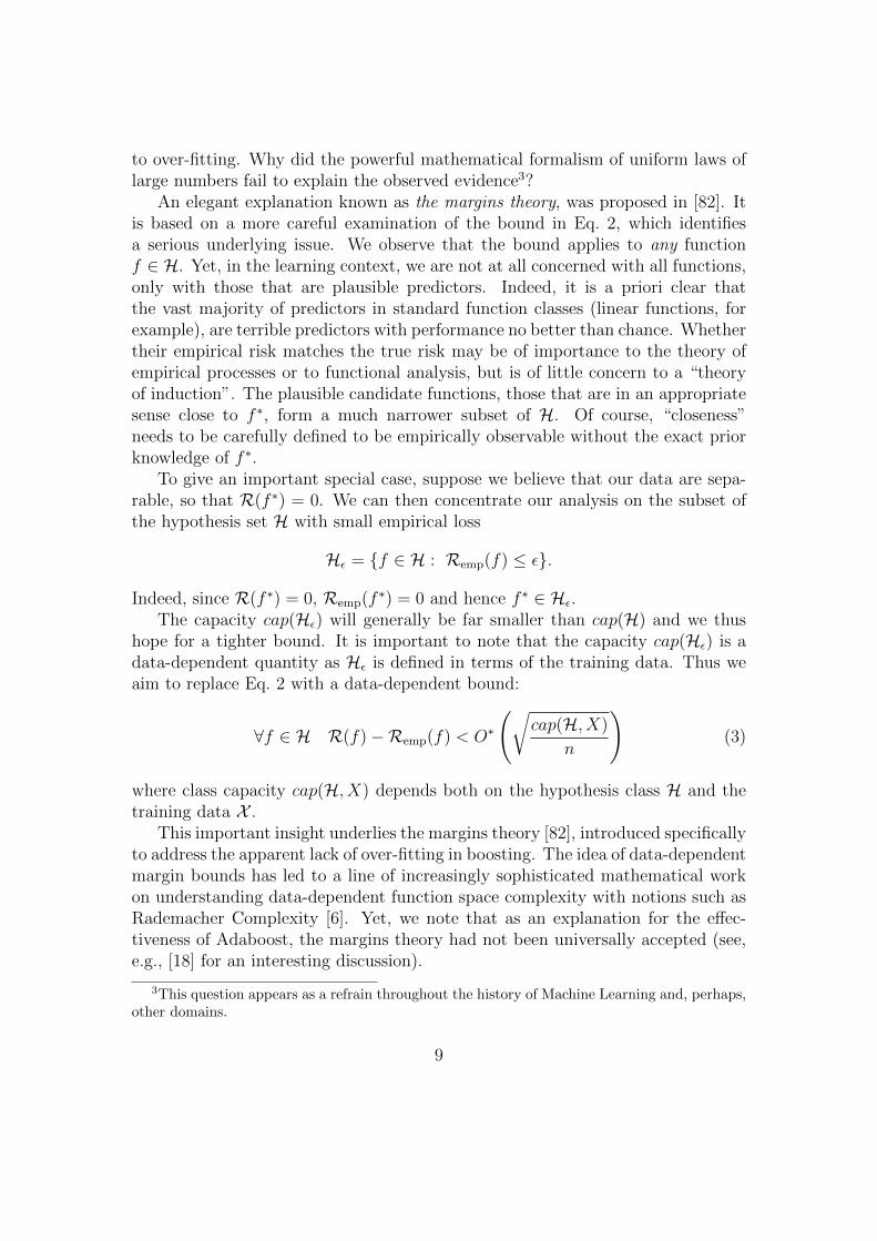
An elegant explanation known as the margins theory, was proposed in [82]. It is based on a more careful examination of the bound in Eq. 2, which identifies a serious underlying issue. We observe that the bound applies to any function f ∈ H. Yet, in the learning context, we are not at all concerned with all functions, only with those that are plausible predictors. Indeed, it is a priori clear that the vast majority of predictors in standard function classes (linear functions, for example), are terrible predictors with performance no better than chance. Whether their empirical risk matches the true risk may be of importance to the theory of empirical processes or to functional analysis, but is of little concern to a “theory of induction”. The plausible candidate functions, those that are in an appropriate sense close to f ∗, form a much narrower subset of H. Of course, “closeness” needs to be carefully defined to be empirically observable without the exact prior knowledge of f ∗.
To give an important special case, suppose we believe that our data are sepa- rable, so that R(f ∗) = 0. We can then concentrate our analysis on the subset of the hypothesis set H with small empirical loss
Hε = {f ∈ H : Remp(f) ≤ ε}.
Indeed, since R(f ∗) = 0, Remp(f ∗) = 0 and hence f ∗ ∈ Hε. The capacity cap(Hε) will generally be far smaller than cap(H) and we thus
hope for a tighter bound. It is important to note that the capacity cap(Hε) is a data-dependent quantity as Hε is defined in terms of the training data. Thus we aim to replace Eq. 2 with a data-dependent bound:
∀f ∈ H R(f)−Remp(f) < O∗
(√ cap(H, X)
n
) (3)
where class capacity cap(H, X) depends both on the hypothesis class H and the training data X .
This important insight underlies the margins theory [82], introduced specifically to address the apparent lack of over-fitting in boosting. The idea of data-dependent margin bounds has led to a line of increasingly sophisticated mathematical work on understanding data-dependent function space complexity with notions such as Rademacher Complexity [6]. Yet, we note that as an explanation for the effectiveness of Adaboost, the margins theory had not been universally accepted (see, e.g., [18] for an interesting discussion).
3This question appears as a refrain throughout the history of Machine Learning and, perhaps, other domains.
9
3.4 What you see is not what you get
It is important to note that the generalization bounds mentioned above, even the data-dependent bounds such as Eq. 3, are “what you see is what you get” (WYSIWYG): the empirical risk that you see in training approximates and bounds the true risk that you expect on unseen data, with the capacity term providing an upper bound on the difference between expected and empirical risk.
Yet, it had gradually become clear (e.g., [70]) that in modern ML, training risk and the true risk were often dramatically different and lacked any obvious connection. In an influential paper [101] the authors demonstrate empirical evidence showing that neural networks trained to have zero classification risk in training do not suffer from significant over-fitting. The authors argue that these and similar observations are incompatible with the existing learning theory and “require rethinking generalization”. Yet, their argument does not fully rule out explanations based on data-dependent bounds such as those in [82] which can produce nontrivial bounds for interpolating predictors if the true Bayes risk is also small.
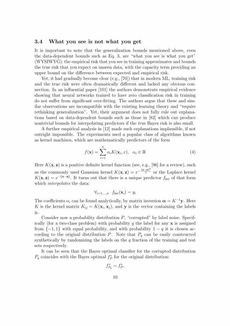
A further empirical analysis in [12] made such explanations implausible, if not outright impossible. The experiments used a popular class of algorithms known as kernel machines, which are mathematically predictors of the form
f(x) = n∑ i=1
αiK(xi, x), αi ∈ R (4)
Here K(x, z) is a positive definite kernel function (see, e.g., [96] for a review), such
as the commonly used Gaussian kernel K(x, z) = e− x−z2
2 or the Laplace kernel K(x, z) = e−x−z. It turns out that there is a unique predictor fker of that form which interpolates the data:
∀i=1,...,n fker(xi) = yi
The coefficients αi can be found analytically, by matrix inversion α = K−1y. Here K is the kernel matrix Kij = K(xi,xj), and y is the vector containing the labels yi.
Consider now a probability distribution P , “corrupted” by label noise. Specif- ically (for a two-class problem) with probability q the label for any x is assigned from {−1, 1} with equal probability, and with probability 1 − q it is chosen according to the original distribution P . Note that Pq can be easily constructed synthetically by randomizing the labels on the q fraction of the training and test sets respectively.
It can be seen that the Bayes optimal classifier for the corrupted distribution Pq coincides with the Bayes optimal f ∗P for the original distribution:
f ∗Pq = f ∗P .
(a) Synthetic, 2-class problem (b) MNIST, 10-class
Figure 2: (From [12]) Interpolated (zero training square loss), “overfitted” (zero training classification error), and Bayes error for datasets with added label noise. y axis: test classification error.
Furthermore, it is easy to check that the 0− 1 loss of the Bayes optimal predictor f ∗P computed with respect to Pq (denoted by RPq) is bounded from below by the noise level:
RPq(f ∗ P ) ≥ q
2
It was empirically shown in [12] that interpolating kernel machines fker,q (see Eq. 4) with common Laplace and Gaussian kernels, trained to interpolate q-corrupted data, generalizes nearly optimally (approaches the Bayes risk) to the similarly corrupted test data. An example of that is shown in4 Fig. 2. In particular, we see that the Laplace kernel tracks the optimal Bayes error very closely, even when as much as 80% of the data are corrupted (i.e., q = 0.8).
Why is it surprising from the WYISWYG bound point of view? For simplicity, suppose P is deterministic (R(f ∗P ) = 0), which is essentially the case [FOOTNOTE MOVED] in Fig. 2, Panel (b). In that case (for a two-class problem), RPq(f
∗ P ) = q
q
2 .
On the other hand Remp(fker,q) = 0 and hence for the left-hand side in Eq. 3 we have
RPq(fker,q)−Remp(fker,q) =0
2
4For a ten-class problem in panel (b), which makes the point even stronger. For simplicity, we only discuss a two-class analysis here.
11
To explain good empirical performance of fker,q, a bound like Eq. 3 needs to be both correct and nontrivial. Since the left hand side is at least q
2 and observing
that RPq(fker,q) is upper bounded by the loss of a random guess, which is 1/2 for a two-class problem, we must have
q
2 ≤
correct
O∗
2 (5)
Note that such a bound would require the multiplicative coefficient in O∗ to be tight within a multiplicative factor 1/q (which is 1.25 for q = 0.8). No such general bounds are known. In fact, typical bounds include logarithmic factors and other multipliers making really tight estimates impossible. More conceptually, it is hard to see how such a bound can exist, as the capacity term would need to “magically” know5 about the level of noise q in the probability distribution. Indeed, a strict mathematical proof of incompatibility of generalization with uniform bounds was recently given in [66] under certain specific settings. The consequent work [4] proved that no good bounds can exist for a broad range of models.
Thus we see that strong generalization performance of classifiers that interpolate noisy data is incompatible with WYSIWYG bounds, independently of the nature of the capacity term.
3.5 Giving up on WYSIWYG, keeping theoretical guarantees
So can we provide statistical guarantees for classifiers that interpolate noisy data? Until very recently there had not been many. In fact, the only common interpo-
lating algorithm with statistical guarantees for noisy data is the well-known 1-NN rule6. Below we will go over a sequence of three progressively more statistically powerful nearest neighbor-like interpolating predictors, starting with the classical 1-NN rule, and going to simplicial interpolation and then to general weighted nearest neighbor/Nadaraya-Watson schemes with singular kernels.
5This applies to the usual capacity definitions based on norms, covering numbers and similar mathematical objects. In principle, it may be possible to “cheat” by letting capacity depend on complex manipulations with the data, e.g., cross-validation. This requires a different type of analysis (see [69, 102] for some recent attempts) and raises the question of what may be considered a useful generalization bound. We leave that discussion for another time.
6In the last two or three years there has been significant progress on interpolating guarantees for classical algorithms like linear regression and kernel methods (see the discussion and refer- ences below). However, traditionally analyses nearly always used regularization which precludes interpolation.
12
3.5.1 The peculiar case of 1-NN
Given an input x, 1-NN(x) outputs the label for the closest (in Euclidean or another appropriate distance) training example.
While the 1-NN rule is among the simplest and most classical prediction rules both for classification and regression, it has several striking aspects which are not usually emphasized in standard treatments:
• It is an interpolating classifier, i.e., Remp(1-NN) = 0.
• Despite “over-fitting”, classical analysis in [20] shows that the classification risk of R(1-NN) is (asymptotically as n → ∞) bounded from above by 2·R(f ∗), where f ∗ is the Bayes optimal classifier defined by Eq. 1.
• Not surprisingly, given that it is an interpolating classifier, there no ERM- style analysis of 1-NN.
It seems plausible that the remarkable interpolating nature of 1-NN had been written off by the statistical learning community as an aberration due to its high excess risk7. As we have seen, the risk of 1-NN can be a factor of two worse than the risk of the optimal classifier. The standard prescription for improving performance is to use k-NN, an average of k nearest neighbors, which no longer interpolates. As k increases (assuming n is large enough), the excess risk decreases as does the difference between the empirical and expected risks. Thus, for large k (but still much smaller than n) we have, seemingly in line with the standard ERM-type bounds,
Remp(k-NN) ≈ R(k-NN) ≈ R(f ∗).
It is perhaps ironic that an outlier feature of 1-NN rule, shared with no other common methods in the classical statistics literature (except for the relatively unknown work [23]), may be one of the cues to understanding modern deep learning.
3.5.2 Geometry of simplicial interpolation and the blessing of dimen- sionality
Yet, a modification of 1-NN different from k-NN maintains its interpolating property while achieving near-optimal excess risk, at least in when the dimension is high. The algorithm is simplicial interpolation [33] analyzed statistically in [10]. Consider a triangulation of the data, x1, . . . ,xn, that is a partition of the convex hull of the data into a set of d-dimensional simplices so that:
7Recall that the excess risk of a classifier f is the difference between the risk of the classifier and the risk of the optimal predictor R(f)−R(f∗).
13
1. Vertices of each simplex are data points.
2. For any data point xi and simplex s, xi is either a vertex of s or does not belong to s.
The exact choice of the triangulation turns out to be unimportant as long as the size of each simplex is small enough. This is guaranteed by, for example, the well-known Delaunay triangulation.
Given a multi-dimensional triangulation, we define fsimp(x), the simplicial in- terpolant, to be a function which is linear within each simplex and such that fsimp(xi) = yi. It is not hard to check that fsimp exists and is unique.
It is worth noting that in one dimension simplicial interpolation based on the Delaunay triangulation is equivalent to 1-NN for classification. Yet, when the dimension d is high enough, simplicial interpolation is nearly optimal both for classification and regression. Specifically, it is was shown in Theorem 3.4 in [10] (Theorem 3.4) that simplicial interpolation benefits from a blessing of dimension- ality. For large d, the excess risk of fsimp decreases with dimension:
R(fsimp)−R(f ∗) = O
) .
Analogous results hold for regression, where the excess risk is similarly the difference between the loss of a predictor and the loss of the (optimal) regression function. Furthermore, for classification, under additional conditions
√ d can be
replaced by ed in the denominator. Why does this happen? How can an interpolating function be nearly optimal
despite the fact that it fits noisy data and why does increasing dimension help? The key observation is that incorrect predictions are localized in the neighbor-
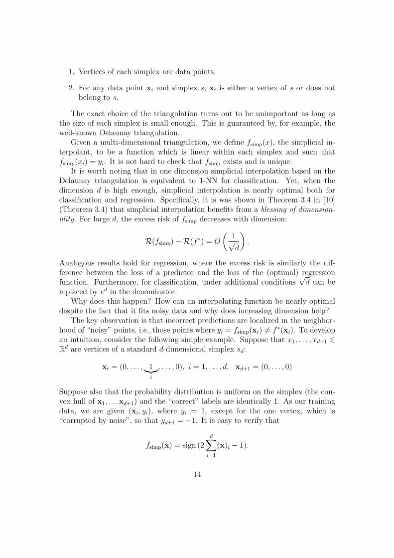
hood of “noisy” points, i.e., those points where yi = fsimp(xi) 6= f ∗(xi). To develop an intuition, consider the following simple example. Suppose that x1, . . . , xd+1 ∈ Rd are vertices of a standard d-dimensional simplex sd:
xi = (0, . . . , 1 i
, . . . , 0), i = 1, . . . , d, xd+1 = (0, . . . , 0)
Suppose also that the probability distribution is uniform on the simplex (the convex hull of x1, . . .xd+1) and the “correct” labels are identically 1. As our training data, we are given (xi, yi), where yi = 1, except for the one vertex, which is “corrupted by noise”, so that yd+1 = −1. It is easy to verify that
fsimp(x) = sign (2 d∑ i=1
(x)i − 1).
Figure 4: Singular kernel for regression. Weighted and interpolated nearest neighbor (wiNN) scheme. Figure credit: Partha Mitra.
We see that fsimp coincides with f ∗ ≡ 1 in the simplex except for the set s1/2 =
{x : ∑d
i=1 xi ≤ 1/2}, which is equal to the simplex 1 2 sd and thus
vol(s1/2) = 1
2d vol(sd)
where fsimp deviates from the optimal predictor f ∗.
We see that the interpolating predictor fsimp
is different from the optimal, but the difference is highly localized around the “noisy” vertex, while at most points within sd their predictions coincide. This is illustrated geometrically in Fig. 3. The reasons for the blessing of dimen- sionality also become clear, as small neighbor- hoods in high dimension have smaller volume relative to the total space. Thus, there is more freedom and flexibility for the noisy points to be localized.
15
3.5.3 Optimality of k-NN with singular weighting schemes
While simplicial interpolation improves on 1-NN in terms of the excess loss, it is still not consistent. In high dimension fsimp is near f ∗ but does not converge to f ∗ as n → ∞. Traditionally, consistency and rates of convergence have been a central object of statistical investigation. The first result in this direction is [23], which showed statistical consistency of a certain kernel regression scheme, closely related to Shepard’s inverse distance interpolation [85].
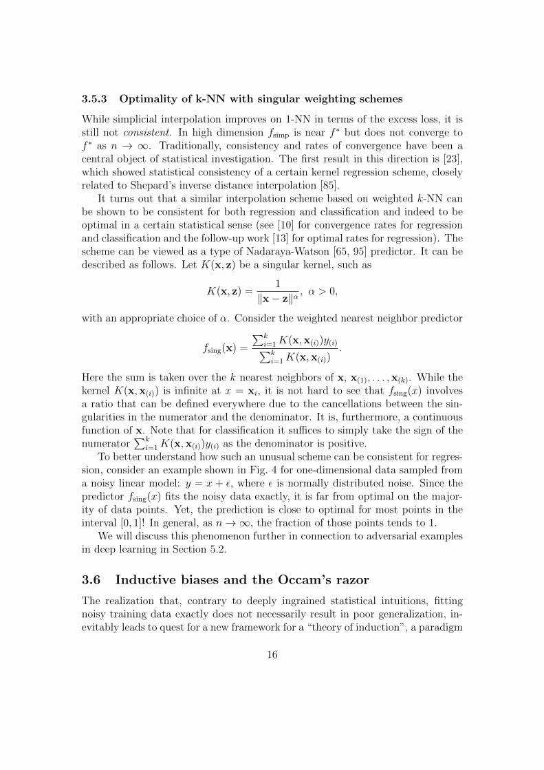
It turns out that a similar interpolation scheme based on weighted k-NN can be shown to be consistent for both regression and classification and indeed to be optimal in a certain statistical sense (see [10] for convergence rates for regression and classification and the follow-up work [13] for optimal rates for regression). The scheme can be viewed as a type of Nadaraya-Watson [65, 95] predictor. It can be described as follows. Let K(x, z) be a singular kernel, such as
K(x, z) = 1
x− zα , α > 0,
with an appropriate choice of α. Consider the weighted nearest neighbor predictor
fsing(x) =
.
Here the sum is taken over the k nearest neighbors of x, x(1), . . . ,x(k). While the kernel K(x,x(i)) is infinite at x = xi, it is not hard to see that fsing(x) involves a ratio that can be defined everywhere due to the cancellations between the sin- gularities in the numerator and the denominator. It is, furthermore, a continuous function of x. Note that for classification it suffices to simply take the sign of the numerator
∑k i=1K(x,x(i))y(i) as the denominator is positive.
To better understand how such an unusual scheme can be consistent for regression, consider an example shown in Fig. 4 for one-dimensional data sampled from a noisy linear model: y = x + ε, where ε is normally distributed noise. Since the predictor fsing(x) fits the noisy data exactly, it is far from optimal on the majority of data points. Yet, the prediction is close to optimal for most points in the interval [0, 1]! In general, as n→∞, the fraction of those points tends to 1.
We will discuss this phenomenon further in connection to adversarial examples in deep learning in Section 5.2.
3.6 Inductive biases and the Occam’s razor
The realization that, contrary to deeply ingrained statistical intuitions, fitting noisy training data exactly does not necessarily result in poor generalization, in- evitably leads to quest for a new framework for a “theory of induction”, a paradigm
16
not reliant on uniform laws of large numbers and not requiring empirical risk to approximate the true risk.
While, as we have seen, interpolating classifiers can be statistically near-optimal or optimal, the predictors discussed above appear to be different from those widely used in ML practice. Simplicial interpolation, weighted nearest neighbor or Nadaraya- Watson schemes do not require training and can be termed direct methods. In contrast, common practical algorithms from linear regression to kernel machines to neural networks are “inverse methods” based on optimization. These algorithms typically rely on algorithmic empirical risk minimization, where a loss function Remp(fw) is minimized via a specific algorithm, such as stochastic gradient descent (SGD) on the weight vector w. Note that there is a crucial and sometimes overlooked difference between the empirical risk minimization as an algorithmic process and the Vapnik’s ERM paradigm for generalization, which is algorithm- independent. This distinction becomes important in over-parameterized regimes, where the hypothesis space H is rich enough to fit any data set8 of cardinality n. The key insight is to separate “classical” under-parameterized regimes where there is typically no f ∈ H, such that R(f) = 0 and “modern” over-parameterized settings where there is a (typically large) set S of predictors that interpolate the training data
S = {f ∈ H : R(f) = 0}. (6)
First observe that an interpolating learning algorithmA selects a specific predictor fA ∈ S. Thus we are faced with the issue of the inductive bias: why do solutions, such as those obtained by neural networks and kernel machines, generalize, while other possible solutions do not9. Notice that this question cannot be answered through the training data alone, as any f ∈ S fits data equally well10. While no conclusive recipe for selecting the optimal f ∈ S yet exists, it can be posited that an appropriate notion of functional smoothness plays a key role in that choice. As argued in [9], the idea of maximizing functional smoothness subject to interpolating the data represents a very pure form of the Occam’s razor (cf. [14, 93]). Usually stated as
Entities should not be multiplied beyond necessity,
the Occam’s razor implies that the simplest explanation consistent with the evidence should be preferred. In this case fitting the data corresponds to consistency
8Assuming that xi 6= xj , when i 6= j. 9The existence of non-generalizing solutions is immediately clear by considering over-
parameterized linear predictors. Many linear functions fit the data – most of them generalize poorly.
10We note that inductive biases are present in any inverse problem. Interpolation simply isolates this issue.
17
“classical” regime
Figure 5: Double descent generalization curve (figure from [9]). Modern and classical regimes are separated by the interpolation threshold.
with evidence, while the smoothest function is “simplest”. To summarize, the “maximum smoothness” guiding principle can be formulated as:
Select the smoothest function, according to some notion of functional smoothness, among those that fit the data perfectly.
We note that kernel machines described above (see Eq. 4) fit this paradigm precisely. Indeed, for every positive definite kernel function K(x, z), there exists a Reproducing Kernel Hilbert Space ( functional spaces, closely related to Sobolev spaces, see [96]) HK , with norm · HK
such that
fHK (7)
We proceed to discuss how this idea may apply to training more complex variably parameterized models including neural networks.
3.7 The Double Descent phenomenon
A hint toward a possible theory of induction is provided by the double descent generalization curve (shown in Fig. 5), a pattern proposed in [9] as a replacement for the classical U-shaped generalization curve (Fig. 1).
When the capacity of a hypothesis class H is below the interpolation threshold, not enough to fit arbitrary data, learned predictors follow the classical U-curve from Figure 1. The shape of the generalization curve undergoes a qualitative change when the capacity of H passes the interpolation threshold, i.e., becomes large enough to interpolate the data. Although predictors at the interpolation threshold typically have high risk, further increasing the number of parameters (capacity of H) leads to improved generalization. The double descent pattern has
18
been empirically demonstrated for a broad range of datasets and algorithms, including modern deep neural networks [9, 67, 87] and observed earlier for linear models [54]. The “modern” regime of the curve, the phenomenon that large number of parameters often do not lead to over-fitting has historically been observed in boosting [82, 98] and random forests, including interpolating random forests [21] as well as in neural networks [16, 70].
Why should predictors from richer classes perform better given that they all fit data equally well? Considering an inductive bias based on smoothness provides an explanation for this seemingly counter-intuitive phenomenon as larger spaces contain will generally contain “better” functions. Indeed, consider a hypothesis space H1 and a larger space H2,H1 ⊂ H2. The corresponding subspaces of interpolating predictors, S1 ⊂ H1 and S2 ⊂ H2, are also related by inclusion: S1 ⊂ S2. Thus, if · s is a functional norm, or more generally, any functional, we see that
min f∈S2
fs
Assuming that · s is the “right” inductive bias, measuring smoothness (e.g., a Sobolev norm), we expect the minimum norm predictor fromH2, fH2 = arg minf∈S2 fs to be superior to that from H1, fH1 = arg minf∈S1 fs.
A visual illustration for double descent and its connection to smoothness is provided in Fig. 6 within the random ReLU family of models in one dimension. A very similar Random Fourier Feature family is described in more mathematical detail below.11 The left panel shows what may be considered a good fit for a model with a small number of parameters. The middle panel, with the number of parameters slightly larger than the minimum necessary to fit the data, shows textbook over-fitting. However increasing the number of parameters further results in a far more reasonably looking curve. While this curve is still piece-wise linear due to the nature of the model, it appears completely smooth. Increasing the number of parameters to infinity will indeed yield a differentiable function (a type of spline), although the difference between 3000 and infinitely many parameters is not visually perceptible. As discussed above, over-fitting appears in a range of models around the interpolation threshold which are complex but yet not complex enough to allow smooth structure to emerge. Furthermore, low complexity parametric models and non-parametric (as the number of parameters approaches infinity) models coexist within the same family on different sides of the interpolation threshold.
Random Fourier features. Perhaps the simplest mathematically and most illuminating example of the double descent phenomenon is based on Random Fourier
11The Random ReLU family consists of piecewise linear functions of the form f(w, x) =∑ k wk min(vkx + bk, 0) where vk, bk are fixed random values. While it is quite similar to RFF,
it produces better visualizations in one dimension.
19
Figure 6: Illustration of double descent for Random ReLU networks in one dimension. Left: Classical under-parameterized regime (3 parameters). Middle: Standard over-fitting, slightly above the interpolation threshold (30 parameters). Right: “Modern” heavily over-parameterized regime (3000 parameters).
Features (RFF ) [78]. The RFF model family Hm with m (complex-valued) parameters consists of functions f : Rd → C of the form
f(w,x) = m∑ k=1
wke √ −1vk,x
where the vectors v1, . . . ,vm are fixed weights with values sampled independently from the standard normal distribution on Rd. The vector w = (w1, . . . , wm) ∈ Cm ∼= R2m consists of trainable parameters. f(w,x) can be viewed as a neural network with one hidden layer of size m and fixed first layer weights (see Eq. 11 below for a general definition of a neural network).
Given data {xi, yi}, i = 1, . . . , n, we can fit fm ∈ Hm by linear regression on the coefficients w. In the overparameterized regime linear regression is given by minimizing the norm under the interpolation constraints12:
fm(x) = arg min f∈Hm, f(w,xi)=yi
w.
lim m→∞
fHK =: fker(x)
Here HK is the Reproducing Kernel Hilbert Space corresponding to the Gaussian kernel K(x, z) = exp(−x − z2) and S ⊂ HK is the manifold of interpolating functions in HK . Note that fker(x) defined here is the same function defined in Eq. 7. This equality is known as the Representer Theorem [43, 96].
We see that increasing the number of parameters m expands the space of interpolating classifiers in Hm and allows to obtain progressively better approximations of the ultimate functional smoothness minimizer fker. Thus adding parameters in
12As opposed to the under-parameterized setting when linear regression it simply minimizes the empirical loss over the class of linear predictors.
20
15
88
4
0
1
10
100
1709
0 10 20 30 40 50 60 7
447
62
0 10 20 30 40 50 60 7
447
62
RFF Min. norm solution hn,
0 10 20 30 40 50 60 Number of Random Fourier Features (×103) (N)
0
8
14
n (%
) RFF
0 10 20 30 40 50 60 Number of Random Fourier Features (×103) (N)
0.0
0.2
0.4
n
RFF
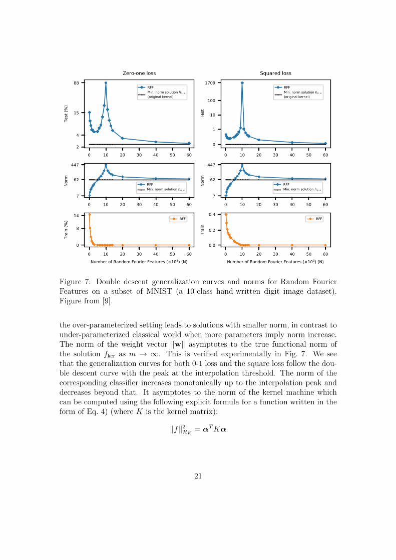
Figure 7: Double descent generalization curves and norms for Random Fourier Features on a subset of MNIST (a 10-class hand-written digit image dataset). Figure from [9].
the over-parameterized setting leads to solutions with smaller norm, in contrast to under-parameterized classical world when more parameters imply norm increase. The norm of the weight vector w asymptotes to the true functional norm of the solution fker as m → ∞. This is verified experimentally in Fig. 7. We see that the generalization curves for both 0-1 loss and the square loss follow the double descent curve with the peak at the interpolation threshold. The norm of the corresponding classifier increases monotonically up to the interpolation peak and decreases beyond that. It asymptotes to the norm of the kernel machine which can be computed using the following explicit formula for a function written in the form of Eq. 4) (where K is the kernel matrix):
f2 HK
3.8 When do minimum norm predictors generalize?
As we have discussed above, considerations of smoothness and simplicity suggest that minimum norm solutions may have favorable generalization properties. This turns out to be true even when the norm does not have a clear interpretation as a smoothness functional. Indeed, consider an ostensibly simple classical regression setup, where data satisfy a linear relation corrupted by noise εi
yi = β∗,xi+ εi, β ∗ ∈ Rd, εi ∈ R, i = 1, . . . , n (8)
In the over-parameterized setting, when d > n, least square regression yields a minimum norm interpolator given by y(x) = βint,x, where
βint = arg min β∈Rd, β,xi=yi, i=1,...,n
β (9)
βint = X†y
where X is the data matrix, y is the vector of labels and X† is the Moore-Penrose (pseudo-)inverse13. Linear regression for models of the type in Eq. 8 is no doubt the oldest14 and best studied family of statistical methods. Yet, strikingly, predictors such as those in Eq. 9, have historically been mostly overlooked, at least for noisy data. Indeed, a classical prescription is to regularize the predictor by, e.g., adding a “ridge” λI to obtain a non-interpolating predictor. The reluc- tance to overfit inhibited exploration of a range of settings where y(x) = βint,x provided optimal or near-optimal predictions. Very recently, these “harmless interpolation” [64] or “benign over-fitting” [5] regimes have become a very active direction of research, a development inspired by efforts to understand deep learning. In particular, the work [5] provided a spectral characterization of models exhibiting this behavior. In addition to the aforementioned papers, some of the first work toward understanding “benign overfitting” and double descent under various linear settings include [11, 34, 61, 99]. Importantly, they demonstrate that when the number of parameters varies, even for linear models over-parametrized predictors are sometimes preferable to any “classical” under-parameterized model.
Notably, even in cases when the norm clearly corresponds to measures of functional smoothness, such as the cases of RKHS or, closely related random feature
13If XXT is invertible, as is usually the case in over-parameterized settings, X† = XT (XXT )−1. In contrast, if XTX is invertible (under the classical under-parameterized setting), X† = (XTX)−1XT . Note that both XXT and XTX matrices cannot be invertible unless X is a square matrix, which occurs at the interpolation threshold.
14Originally introduced by Gauss and, possibly later, Legendre! See [88].
22
maps, the analyses of interpolation for noisy data are subtle and have only recently started to appear, e.g., [49, 60]. For a far more detailed overview of the progress on interpolation in linear regression and kernel methods see the parallel Acta Numerica paper [7].
3.9 Alignment of generalization and optimization in linear and kernel models
While over-parameterized models have manifolds of interpolating solutions, minimum norm solutions, as we have discussed, have special properties which may be conducive to generalization. For over-parameterized linear and kernel models15
there is a beautiful alignment of optimization and minimum norm interpolation: gradient descent GD or Stochastic Gradient Descent (SGD) initialized at the origin can be guaranteed to converge to βint defined in Eq. 9. To see why this is the case we make the following observations:
• βint ∈ T , where T = Span {x1, . . . , xn} is the span of the training examples (or their feature embeddings in the kernel case). To see that, verify that if βint /∈ T , orthogonal projection of βint onto T is an interpolating predictor with even smaller norm, a contradiction to the definition of βint.
• The (affine) subspace of interpolating predictors S (Eq. 6) is orthogonal to T and hence {βint} = S ∩ T .
These two points together are in fact a version of the Representer theorem briefly discussed in Sec. 3.7.
Consider now gradient descent for linear regression initialized at within the span of training examples β0 ∈ T . Typically, we simply choose β0 = 0 as the origin has the notable property of belonging to the span of any vectors. It can be easily verified that the gradient of the loss function at any point is also in the span of the training examples and thus the whole optimization path lies within T . As the gradient descent converges to a minimizer of the loss function, and T is a closed set, GD must converge to the minimum norm solution βint. Remarkably, in the over-parameterized settings convergence to βint is true for SGD, even with a fixed learning rate (see Sec. 4.4). In contrast, under-parameterized SGD with a fixed learning rate does not converge at all.
1516
23
3.10 Is deep learning kernel learning? Transition to linearity in wide neural networks.
But how do these ideas apply to deep neural networks? Why are complicated non-linear systems with large numbers of parameters able to generalize to unseen data?
It is important to recognize that generalization in large neural networks is a robust pattern that holds across multiple dimensions of architectures, optimization methods and datasets17. As such, the ability of neural networks to generalize to unseen data reflects a fundamental interaction between the mathematical structures underlying neural function spaces, algorithms and the nature of our data. It can be likened to the gravitational force holding the Solar System, not a momentary alignment of the planets.
This point of view implies that understanding generalization in complex neural networks has to involve a general principle, relating them to more tractable mathematical objects. A prominent candidate for such an object are kernel machines and their corresponding Reproducing Kernel Hilbert Spaces. As we discussed above, Random Fourier Features-based networks, a rather specialized type of neural architectures, approximate Gaussian kernel machines. Perhaps general neural networks can also be tied to kernel machines? Strikingly, it turns out to be the case indeed, at least for some classes of neural networks.
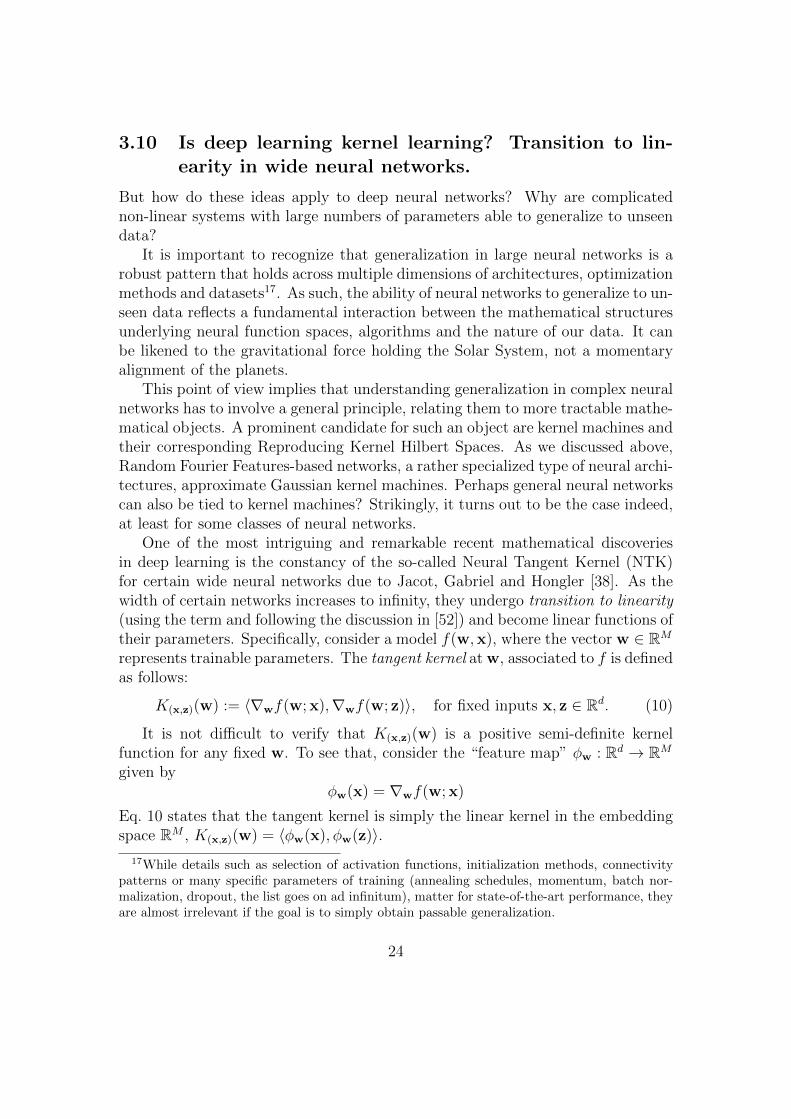
One of the most intriguing and remarkable recent mathematical discoveries in deep learning is the constancy of the so-called Neural Tangent Kernel (NTK) for certain wide neural networks due to Jacot, Gabriel and Hongler [38]. As the width of certain networks increases to infinity, they undergo transition to linearity (using the term and following the discussion in [52]) and become linear functions of their parameters. Specifically, consider a model f(w,x), where the vector w ∈ RM
represents trainable parameters. The tangent kernel at w, associated to f is defined as follows:
K(x,z)(w) := ∇wf(w; x),∇wf(w; z), for fixed inputs x, z ∈ Rd. (10)
It is not difficult to verify that K(x,z)(w) is a positive semi-definite kernel function for any fixed w. To see that, consider the “feature map” φw : Rd → RM
given by φw(x) = ∇wf(w; x)
Eq. 10 states that the tangent kernel is simply the linear kernel in the embedding space RM , K(x,z)(w) = φw(x), φw(z).
17While details such as selection of activation functions, initialization methods, connectivity patterns or many specific parameters of training (annealing schedules, momentum, batch nor- malization, dropout, the list goes on ad infinitum), matter for state-of-the-art performance, they are almost irrelevant if the goal is to simply obtain passable generalization.
24
The surprising and singular finding of [38] is that for a range of infinitely wide neural network architectures with linear output layer, φw(x) is independent of w in a ball around a random “initialization” point w0. That can be shown to be equivalent to the linearity of f(w,x) in w (and hence transition to linearity in the limit of infinite width):
f(w,x) = w −w0, φw0(x)+ f(w0,x)
Note that f(w,x) is not a linear predictor in x, it is a kernel machine, linear in terms of the parameter vector w ∈ RM . Importantly, f(w,x) has linear training dynamics and that is the way this phenomenon is usually described in the machine learning literature (e.g., [47]) . However the linearity itself is a property of the model unrelated to any training procedure18.
To understand the nature of this transition to linearity consider the Taylor ex- pansion of f(w,x) around w0 with the Lagrange remainder term in a ball B⊂ RM
of radius R around w0. For any w ∈ B there is ξ ∈ B so that
f(w,x) = f(w0,x) + w −w0, φw0(x)+ 1
2 w −w0, H(ξ)(w −w0)
We see that the deviation from the linearity is bounded by the spectral norm of the Hessian:
sup w∈B
2 sup ξ∈B H(ξ)
A general (feed-forward) neural network with L hidden layers and a linear output layer is a function defined recursively as:
α(0) = x,
α(l) = φl(W (l) ∗α(l−1)),α ∈ Rdl ,W(l) ∈ Rdl×dl−1 , l = 1, 2, . . . , L,
f(w,x) = 1√ m
vTα(L),v ∈ RdL (11)
The parameter vector w is obtained by concatenation of all weight vectors w = (w(1), . . . ,w(L),v) and the activation functions φl are usually applied coordinate- wise. It turns out these, seemingly complex, non-linear systems exhibit transition to linearity under quite general conditions (see [52]), given appropriate random
18This is a slight simplification as for any finite width the linearity is only approximate in a ball of a finite radius. Thus the optimization target must be contained in that ball. For the square loss it is always the case for sufficiently wide network. For cross-entropy loss it is not generally the case, see Section 5.1.
25
initialization w0. Specifically, it can be shown that for a ball B of fixed radius around the initialization w0 the spectral norm of the Hessian satisfies
sup ξ∈B H(ξ) ≤ O∗
( 1√ m
l=1,...,L (dl) (12)
It is important to emphasize that linearity is a true emerging property of large systems and does not come from the scaling of the function value with the increasing width m. Indeed, for any m the value of the function at initialization and its gradient are all of order 1, f(w, x) = (1), ∇f(w, x) = (1).
Two-layer network: an illustration. To provide some intuition for this structural phenomenon consider a particularly simple case of a two-layer neural network with fixed second layer. Let the model f(w, x), x ∈ R be of the form
f(w, x) = 1√ m
viα(wix), (13)
For simplicity, assume that vi ∈ {−1, 1} are fixed and wi are trainable parameters. It is easy to see that in this case the Hessian H(w) is a diagonal matrix with
(H)ii = 1√ m vi d2α(wi x)
d2wi = ± 1√
a
∇wf =
√ 1
m
∑ i
b

Assuming that w is such, that α′(wix) and α′′(wjx) are of all of the same order, from the relationship between 2-norm and ∞-norm in Rm we expect
b ∼ √ m a∞.
26
Thus, we see that the structure of the Hessian matrix forces its spectral norm to be a factor of
√ m smaller compared to the gradient. If (following a common
practice) wi are sampled iid from the standard normal distribution
∇wf = √ K(w,w)(x) = (1), H(w) = O
( 1√ m
) (15)
If, furthermore, the second layer weights vi are sampled with expected value zero, f(w, x) = O(1). Note that to ensure the transition to linearity we need for the scaling in Eq. 15 to hold in ball of radius O(1) around w (rather than just at the point w), which, in this case, can be easily verified.
The example above illustrates how the transition to linearity is the result of the structural properties of the network (in this case the Hessian is a diagonal matrix) and the difference between the 2-norm ind ∞-norm in a high-dimensional space. For general deep networks the Hessian is no longer diagonal, and the argument is more involved, yet there is a similar structural difference between the gradient and the Hessian related to different scaling of the 2 and ∞ norms with dimension.
Furthermore, transition to linearity is not simply a property of large systems. Indeed, adding a non-linearity at the output layer, i.e., defining
g(w, x) = φ(f(w, x))
where f(w, x) is defined by Eq. 13 and φ is any smooth function with non-zero second derivative breaks the transition to linearity independently of the width m and the function φ. To see that, observe that the Hessian of g, Hg can be written, in terms of the gradient and Hessian of f , (∇wf and H(w), respectively) as
Hg(w) = φ′(f) H(w) O(1/
√ m)
(16)
We see that the second term in Eq. 16 is of the order ∇wf2 = (1) and does not scale with m. Thus the transition to linearity does not occur and the tangent kernel does not become constant in a ball of a fixed radius even as the width of the network tends to infinity. Interestingly, introducing even a single narrow “bottleneck” layer has the same effect even if the activation functions in that layer are linear (as long as some activation functions in at least one of the deeper layers are non-linear).
As we will discuss later in Section 4, the transition to linearity is not needed for optimization, which makes this phenomenon even more intriguing. Indeed, it is possible to imagine a world where the transition to linearity phenomenon does not exist, yet neural networks can still be optimized using the usual gradient-based methods.
27
It is thus even more fascinating that a large class of very complex functions turn out to be linear in parameters and the corresponding complex learning algorithms are simply training kernel machines. In my view this adds significantly to the evidence that understanding kernel learning is a key to deep learning as we argued in [12]. Some important caveats are in order. While it is arguable that deep learning may be equivalent to kernel learning in some interesting and practical regimes, the jury is still out on the question of whether this point of view can provide a conclusive understanding of generalization in neural networks. Indeed a considerable amount of recent theoretical work has been aimed at trying to understand regimes (sometimes called the “rich regimes”, e.g., [30, 97]) where the transition to linearity does not happen and the system is non-linear throughout the training process. Other work (going back to [94]) argues that there are theoretical barriers separating function classes learnable by neural networks and kernel machines [1, 75]. Whether these analyses are relevant for explaining empirically observed behaviours of deep networks still requires further exploration.
Please also see some discussion of these issues in Section 6.2.
4 The wonders of optimization
The success of deep learning has heavily relied on the remarkable effectiveness of gradient-based optimization methods, such as stochastic gradient descent (SGD), applied to large non-linear neural networks. Classically, finding global minima in non-convex problems, such as these, has been considered intractable and yet, in practice, neural networks can be reliably trained.
Over-parameterization and interpolation provide a distinct perspective on optimization. Under-parameterized problems are typically locally convex around their local minima. In contrast, over-parameterized non-linear optimization landscapes are generically non-convex, even locally. Instead, as we will argue, throughout most (but not all) of the parameter space they satisfy the Polyak - Lojasiewicz condition, which guarantees both existence of global minima within any sufficiently large ball and convergence of gradient methods, including GD and SGD.
Finally, as we discuss in Sec. 4.4, interpolation sheds light on a separate empirically observed phenomenon, the striking effectiveness of mini-batch SGD (ubiquitous in applications) in comparison to the standard gradient descent.
4.1 From convexity to the PL* condition
Mathematically, interpolation corresponds to identifying w so that
f(w,xi) = yi, i = 1, . . . , n,xi ∈ Rd,w ∈ RM .
28
This is a system of n equations with M variables. Aggregating these equations into a single map,
F (w) = (f(w,x1), . . . , f(w,xn)), (17)
and setting y = (y1, . . . , yn), we can write that w is a solution for a single equation
F (w) = y, F : RM → Rn. (18)
When can such a system be solved? The question posed in such generality ini- tially appears to be absurd. A special case, that of solving systems of polynomial equations, is at the core of algebraic geometry, a deep and intricate mathematical field. And yet, we can often easily train non-linear neural networks to fit arbitrary data [101]. Furthermore, practical neural networks are typically trained using simple first order gradient-based methods, such as stochastic gradient descent (SGD).
The idea of over-parameterization has recently emerged as an explanation for this phenomenon based on the intuition that a system with more variables than equations can generically be solved. We first observe that solving Eq. 18 (assuming a solution exists) is equivalent to minimizing the loss function
L(w) = F (w)− y2.
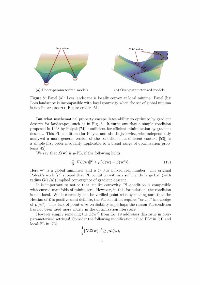
This is a non-linear least squares problem, which is well-studied under classical under-parameterized settings (see [72], Chapter 10). What property of the over- parameterized optimization landscape allows for effective optimization by gradient descent (GD) or its variants? It is instructive to consider a simple example in Fig. 8 (from [51]). The left panel corresponds to the classical regime with many isolated local minima. We see that for such a landscape there is little hope that a local method, such as GD can reach a global optimum. Instead we expect it to converge to a local minimum close to the initialization point. Note that in a neighborhood of a local minimizer the function is convex and classical convergence analyses apply.
A key insight is that landscapes of over-parameterized systems look very dif- ferently, like the right panel in Fig 8b. We see that there every local minimum is global and the manifold of minimizers S has positive dimension. It is important to observe that such a landscape is incompatible with convexity even locally. Indeed, consider an arbitrary point s ∈ S inside the insert in Fig 8b. If L(w) is convex in any ball B ⊂ S around s, the set of minimizers within that neighborhood, B ∩ S must be a a convex set in RM . Hence S must be a locally linear manifold near s for L to be locally convex. It is, of course, not the case for general systems and cannot be expected, even at a single point.
Thus, one of the key lessons of deep learning in optimization: Convexity, even locally, cannot be the basis of analysis for over-parameterized systems.
29
(a) Under-parameterized models (b) Over-parameterized models
Figure 8: Panel (a): Loss landscape is locally convex at local minima. Panel (b): Loss landscape is incompatible with local convexity when the set of global minima is not linear (insert). Figure credit: [51].
But what mathematical property encapsulates ability to optimize by gradient descent for landscapes, such as in Fig. 8. It turns out that a simple condition proposed in 1963 by Polyak [74] is sufficient for efficient minimization by gradient descent. This PL-condition (for Polyak and also Lojasiewicz, who independently analyzed a more general version of the condition in a different context [53]) is a simple first order inequality applicable to a broad range of optimization problems [42].
We say that L(w) is µ-PL, if the following holds:
1
2 ∇L(w)2 ≥ µ(L(w)− L(w∗)), (19)
Here w∗ is a global minimizer and µ > 0 is a fixed real number. The original Polyak’s work [74] showed that PL condition within a sufficiently large ball (with radius O(1/µ)) implied convergence of gradient descent.
It is important to notice that, unlike convexity, PL-condition is compatible with curved manifolds of minimizers. However, in this formulation, the condition is non-local. While convexity can be verified point-wise by making sure that the Hessian of L is positive semi-definite, the PL condition requires ”oracle” knowledge of L(w∗). This lack of point-wise verifiability is perhaps the reason PL-condition has not been used more widely in the optimization literature.
However simply removing the L(w∗) from Eq. 19 addresses this issue in over- parameterized settings! Consider the following modification called PL* in [51] and local PL in [73].
1
30
Figure 9: The loss function L(w) is µ-PL* inside the shaded domain. Singular set correspond to parameters w with degenerate tangent kernel K(w). Every ball of radius O(1/µ) within the shaded set intersects with the set of global minima of L(w), i.e., solutions to F (w) = y. Figure credit: [51].
It turns out that PL* condition in a ball of sufficiently large radius implies both existence of an interpolating solution within that ball and exponential convergence of gradient descent and, indeed, stochastic gradient descent.
It is interesting to note that PL* is not a useful concept in under-parameterized settings – generically, there is no solution to F (w) = y and thus the condition cannot be satisfied along the whole optimization path. On the other hand, the condition is remarkably flexible – it naturally extends to Riemannian manifolds (we only need the gradient to be defined) and is invariant under non-degenerate coordinate transformations.
4.2 Condition numbers of nonlinear systems
Why do over-parameterized systems satisfy the PL* condition? The reason is closely related to the Tangent Kernel discussed in Section 3.10. Consider the tangent kernel of the map F (w) defined as n× n matrix valued function
K(w) = DF T (w)×DF (w), DF (w) ∈ RM×n
where DF is the differential of the map F . It can be shown for the square loss L(w) satisfies the PL*- condition with µ = λmin(K). Note that the rank of K is less or equal to M . Hence, if the system is under-parameterized, i.e., M < n, λmin(K)(w) ≡ 0 and the corresponding PL* condition is always trivial.
31
In contrast, when M ≥ n, we expect λmin(K)(w) > 0 for generic w. More precisely, by parameter counting, we expect that the set of of w with singular Tangent Kernel {w ∈ RM : λmin(K)(w) = 0} is of co-dimension M −n+ 1, which is exactly the amount of over-parameterization. Thus, we expect that large subsets of the space RM have eigenvalues separated from zero, λmin(K)(w) ≥ µ. This is depicted graphically in Fig. 9 (from [51]). The shaded areas correspond to the sets where the loss function is µ-PL*. In order to make sure that solution to the Eq. 17 exists and can be achieved by Gradient Descent, we need to make sure that
λmin(K)(w) > µ in a ball of radius O (
1 µ
) . Every such ball in the shaded area
contains solutions of Eq. 17 (global minima of the loss function). But how can an analytic condition, like a lower bound on the smallest eigen-
value of the tangent kernel, be verified for models such as neural networks?
4.3 Controlling PL* condition of neural networks
As discussed above and graphically illustrated in Fig. 9, we expect over-parameterized systems to satisfy the PL* condition over most of the parameter space. Yet, ex- plicitly controlling µ = λmin(K) in a ball of a certain radius can be subtle. We can identify two techniques which help establish such control for neural networks and other systems. The first one, the Hessian control, uses the fact that near- linear systems are well-conditioned in a ball, provided they are well-conditioned at the origin. The second, transformation control, is based on the observation that well-conditioned systems stay such under composition with “benign” transformations. Combining these techniques can be used to prove convergence of randomly initialized wide neural networks.
4.3.1 Hessian control
Transition to linearity, discussed in Section 3.10, provides a powerful (if somewhat crude) tool for controlling λmin(K) for wide networks. The key observation is that K(w) is closely related to the first derivative of F at w. Thus the change of K(w) from the initialization K(w0) can be bounded in terms of the norm of the Hessian H, the second derivative of F using, essentially, the mean value theorem. We can bound the operator norm to get the following inequality (see [52]):
∀w ∈ BR K(w)−K(w0) ≤ O
( Rmax
) (20)
where BR is a ball of radius R around w0. Using standard eigenvalue perturbation bounds we have
∀w ∈ BR |λmin(K)(w)− λmin(K)(w0)| ≤ O
( Rmax
) (21)
32
Recall (Eq. 12) that for networks of widthm with linear last layer H = O(1/ √ m).
On the other hand, it can be shown (e.g., [25] and [24] for shallow and deep networks respectively) that λmin(K)(w0) = O(1) and is essentially independent of the width. Hence Eq. 21 guarantees that given any fixed radius R, for a sufficiently wide network λmin(K)(w) is separated from zero in the ball BR. Thus the loss function satisfies the PL* condition in BR. As we discussed above, this guarantees the existence of global minima of the loss function and convergence of gradient descent for wide neural networks with linear output layer.
4.3.2 Transformation control
Another way to control the condition number of a system is by representing it as a composition of two or more well-conditioned maps.
Informally, due to the chain rule, if F is well conditioned, so is φ F ψ(w), where
φ : Rn → Rn, ψ : Rm → Rm
are maps with non-degenerate Jacobian matrices. In particular, combining Hessian control with transformation control, can be
used to prove convergence for wide neural networks with non-linear last layer [52].
4.4 Efficient optimization by SGD
We have seen that over-parameterization helps explain why Gradient Descent can reach global minima even for highly non-convex optimization landscapes. Yet, in practice, GD is rarely used. Instead, mini-batch stochastic methods, such as SGD or Adam [44] are employed almost exclusively. In its simplest form, mini-batch SGD uses the following update rule:
wt+1 = wt − η∇
) (22)
Here {(xi1 , yi1), . . . , (xim , yim)} is a mini-batch, a subset of the training data of size m, chosen at random or sequentially and η > 0 is the learning rate.
At a first glance, from a classical point of view, it appears that GD should be preferable to SGD. In a standard convex setting GD converges at an exponential (referred as linear in the optimization literature) rate, where the loss function decreases exponentially with the number of iterations. In contrast, while SGD requires a factor of n
m less computation than GD per iteration, it converges at a
far slower sublinear rate (see [17] for a review), with the loss function decreasing proportionally to the inverse of the number of iterations. Variance reduction techniques [22, 40, 80] can close the gap theoretically but are rarely used in practice.
33
As it turns out, interpolation can explain the surprising effectiveness of plain SGD compared to GD and other non-stochastic methods19
The key observation is that in the interpolated regime SGD with fixed step size converges exponentially fast for convex loss functions. The results showing exponential convergence of SGD when the optimal solution minimizes the loss function at each point go back to the Kaczmarz method [41] for quadratic functions, more recently analyzed in [89]. For the general convex case, it was first shown in [62]. The rate was later improved in [68].
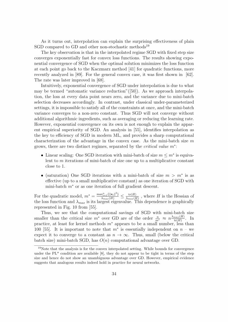
Intuitively, exponential convergence of SGD under interpolation is due to what may be termed “automatic variance reduction”([50]). As we approach interpolation, the loss at every data point nears zero, and the variance due to mini-batch selection decreases accordingly. In contrast, under classical under-parameterized settings, it is impossible to satisfy all of the constraints at once, and the mini-batch variance converges to a non-zero constant. Thus SGD will not converge without additional algorithmic ingredients, such as averaging or reducing the learning rate. However, exponential convergence on its own is not enough to explain the apparent empirical superiority of SGD. An analysis in [55], identifies interpolation as the key to efficiency of SGD in modern ML, and provides a sharp computational characterization of the advantage in the convex case. As the mini-batch size m grows, there are two distinct regimes, separated by the critical value m∗:
• Linear scaling: One SGD iteration with mini-batch of size m ≤ m∗ is equivalent to m iterations of mini-batch of size one up to a multiplicative constant close to 1.
• (saturation) One SGD iterations with a mini-batch of size m > m∗ is as effective (up to a small multiplicative constant) as one iteration of SGD with mini-batch m∗ or as one iteration of full gradient descent.
For the quadratic model, m∗ = maxn
i=1{xi2} λmax(H)
≤ tr(H) λmax(H)
, where H is the Hessian of the loss function and λmax is its largest eigenvalue. This dependence is graphically represented in Fig. 10 from [55].
Thus, we see that the computational savings of SGD with mini-batch size smaller than the critical size m∗ over GD are of the order n
m∗ ≈ nλmax(H)
tr(H) . In
practice, at least for kernel methods m∗ appears to be a small number, less than 100 [55]. It is important to note that m∗ is essentially independent on n – we expect it to converge to a constant as n → ∞. Thus, small (below the critical batch size) mini-batch SGD, has O(n) computational advantage over GD.
19Note that the analysis is for the convex interpolated setting. While bounds for convergence under the PL* condition are available [8], they do not appear to be tight in terms of the step size and hence do not show an unambiguous advantage over GD. However, empirical evidence suggests that analogous results indeed hold in practice for neural networks.
34
Figure 10: Number of iterations with batch size 1 (the y axis) equivalent to one iteration with batch size m. Critical batch size m∗ separates linear scaling and regimes. Figure credit: [55].
To give a simple realistic example, if n = 106 and m∗ = 10, SGD has a factor of 105 advantage over GD, a truly remarkable improvement!
5 Odds and ends
5.1 Square loss for training in classification?
The attentive reader will note that most of our optimization discussions (as well as in much of the literature) involved the square loss. While training using the square loss is standard for regression tasks, it is rarely employed for classification, where the cross-entropy loss function is the standard choice for training. For two class problems with labels yi ∈ {1,−1} the cross-entropy (logistic) loss function is defined as
lce(f(xi), yi) = log ( 1 + e−yif(xi)
) (23)
A striking aspect of cross-entropy is that in order to achieve zero loss we need to have yif(xi) =∞. Thus, interpolation only occurs at infinity and any optimization procedure would eventually escape from a ball of any fixed radius. This presents difficulties for optimization analysis as it is typically harder to apply at infinity. Furthermore, since the norm of the solution vector is infinite, there can be no transition to linearity on any domain that includes the whole optimization path, no matter how wide our network is and how tightly we control the Hessian norm (see Section 3.10). Finally, analyses of cross-entropy in the linear case [39] suggest
35
that convergence is much slower than for the square loss and thus we are unlikely to approach interpolation in practice.
Thus the use of the cross-entropy loss leads us away from interpolating solutions and toward more complex mathematical analyses. Does the prism of interpolation fail us at this junction?
The accepted justification of the cross-entropy loss for classification is that it is a better “surrogate” for the 0-1 classification loss than the square loss (e.g., [31], Section 8.1.2). There is little theoretical analysis supporting this point of view. To the contrary, very recent theoretical works [58, 63, 92] prove that in certain over-parameterized regimes, training using the square loss for classification is at least as good or better than using other loss functions. Furthermore, extensive empirical evaluations conducted in [36] show that modern neural architectures trained with the square loss slightly outperform same architectures trained with the cross-entropy loss on the majority of tasks across several application domains including Natural Language Processing, Speech Recognition and Computer Vision.
A curious historical parallel is that current reliance on cross-entropy loss in classification reminiscent of the predominance of the hinge loss in the era of the Support Vector Machines (SVM). At the time, the prevailing intuition had been that the hinge loss was preferable to the square loss for training classifiers. Yet, the empirical evidence had been decidedly mixed. In his remarkable 2002 thesis [79], Ryan Rifkin conducted an extensive empirical evaluation and concluded that “the performance of the RLSC [square loss] is essentially equivalent to that of the SVM [hinge loss] across a wide range of problems, and the choice between the two should be based on computational tractability considerations”.
We see that interpolation as a guiding principle points us in a right direction yet again. Furthermore, by suggesting the square loss for classification, it reveals shortcomings of theoretical intuitions and the pitfalls of excessive belief in empirical best practices.
5.2 Interpolation and adversarial examples
A remarkable feature of modern neural networks is existence of adversarial examples. It was observed in [91] that by adding a small, visually imperceptible, perturbation of the pixels, an image correctly classified as “dog” can be moved to class “ostrich” or to some other obviously visually incorrect class. Far from being an isolated curiosity, this turned out to be a robust and ubiquitous property among different neural architectures. Indeed, modifying a single, carefully selected, pixel is frequently enough to coax a neural net into misclassifying an image [90].
The full implications and mechanisms for the emergence of adversarial examples are not yet fully understood and are an active area of research. Among other things, the existence and pervasiveness of adversarial examples points to the lim-
36
Figure 11: Raisin bread: The “raisins” are basins where the interpolating predictor fint disagrees with the optimal predictor f ∗, surrounding “noisy” data points. The union of basins is an everywhere dense set of zero measure (as n→∞).
itations of the standard iid models as these data are not sampled from the same distribution as the training set. Yet, it can be proved mathematically that adversarial examples are unavoidable for interpolating classifiers in the presence of label noise [10] (Theorem 5.1). Specifically, suppose fint is an interpolating classifier and let x be an arbitrary point. Assume that fint(x) = y is a correct prediction. Given a sufficiently large dataset, there will be at least one ”noisy” point xi, yi,, such as f ∗(xi) 6= yi, in a small neighborhood of x and thus a small perturbation of x can be used to flip the label.
If, furthermore, fint is a consistent classifier, such as predictors discussed in Section 3.5.3, it will approach the optimal predictor f ∗ as the data size grows.
Specifically, consider the set where predictions of fint differ from the optimal classification
Sn = {x : f ∗(x) 6= fint(x)}
From consistency, we have lim n→∞
µ(Sn) = 0
where µ is marginal probability measure of the data distribution. On the other hand, as n → ∞, Sn becomes a dense subset of the data domain. This can be thought of as a raisin bread20. The are the incorrect classification basins around each misclassified example, i.e., the areas where the output of fint differs from f ∗. While the seeds permeate the bread, they occupy negligible volume inside.
20Any similarity to the “plum pudding” model of the atom due to J.J.Thompson is purely coincidental.
37
This picture is indeed consistent with the extensive empirical evidence for neural networks. A random perturbation avoids adversarial “raisins” [26], yet they are easy to find by targeted optimization methods such as PCG [57]. I should point out that there are also other explanations for adversarial examples [37]. It seems plausible that several mathematical effects combine to produce adversarial examples.
6 Summary and thoughts
We proceed to summarize the key points of this article and conclude with a discussion of machine learning and some key questions still unresolved.
6.1 The two regimes of machine learning
The sharp contrast between the “classical” and “modern” regimes in machine learning, separated by the interpolation threshold, in various contexts, has been a central aspect of the discussion in this paper. A concise summary of some of these differences in a single table is given below.
Capacity
Risk
Classical (under-parameterized) Modern (over-parameterized)
Generalization curve U-shaped Descending
Optimal model Bottom of U (hard to find) Any large model (easy to find)
Optimization landscape: Locally convex Not locally convex Minimizers locally unique Manifolds of minimizers
Satisfies PL* condition
GD/SGD convergence GD converges to local min GD/SGD converge to global min SGD w. fixed learning rate does SGD w. fixed learning rate
not converge converges exponentially
38
6.2 Through a glass darkly
In conclusion, it may be worthwhile to discuss some of the many missing or nebu- lous mathematical pieces in the gradually coalescing jigsaw puzzle of deep learning.
Inverse and direct methods. To my mind, the most puzzling question of machine learning is why inverse methods, requiring optimization or inversion, generally perform better than direct methods such as nearest neighbors. For example, a kernel machine with a positive definite kernel K(x, z), appears to perform consistently and measurably better than a Nadaraya-Watson (NW) classifier using the same kernel (or the same family of kernels), despite the fact that both have the same functional form
f(x) = n∑ i=1
αiK(xi,x), αi ∈ R
The difference is that for a kernel machine α = (K)−1y, which requires a kernel matrix inversion21, while NW (for classification) simply puts α = y.
The advantage of inverse methods appears to be a broad empirical pattern, manifested, in particular, by successes of neural networks. Indeed, were it not the case that inverse methods performed significantly better, the Machine Learning landscape would look quite different – there would be far less need for optimization techniques and, likely, less dependence on the availability of computational resources. I am not aware of any compelling theoretical analyses to explain this remarkable empirical difference.
Why does optimization align with statistics? A related question is that of the inductive bias. In over-parameterized settings, optimization methods, such as commonly used SGD and Adam [44], select a specific point w∗ in the set of parameters S corresponding to interpolating solutions. In fact, given that w∗ depends on the initialization typically chosen randomly, e.g., from a normal distribution, we should view w∗ as sampled from some induced probability distribution µ on the subset of S reachable by optimization.
Why do parameters sampled from µ consistently generalize to data

Date post:	31-Dec-2021
Category:	Documents
Author:	others
View:	0 times
Download:	0 times

Fit without fear: remarkable mathematical phenomena of ...

Documents

Remarkable Leaders

Levels, Causes and Consequences of the Fear Phenomena: … · 2014. 3. 19. · Levels, Causes and Consequences of the Fear Phenomena: Findinngs from a Pilot Study in Tanzania. 1.

Fear of Fear Anxiety and Burnout

Australia’s #1 EA conference, with the most relevant and · people to overcome their fear and find their voice through public speaking training. This is a remarkable transition

Life’s Most Common Fears Fear of Loss Fear of Failure Fear of Rejection Fear of the Unknown.

Georgia: Remarkable Reforms and Shifting Norms · 2020-05-04 · phenomena, and hold the potential to entrench vicious cycles of behavior But as this paper will examine: Social norms

1.2 Electromagnetic Radiation and Quantum Phenomena Quantum Phenomena

Remove ReMarkable Ads (Removal Guide), How To Remove ReMarkable Ads

remarkable leadership

Real Estate Booms and Banking Busts—An International Perspective€¦ · banking crises may occur without real estate cycles. But the two phenomena are correlated in a remarkable

Remarkable Nature...

Floco Tausin, Entoptic phenomena as universal trance phenomena · Entoptic phenomena as universal trance phenomena ... entoptic phenomena and shamanism. Abstract art, ... Shamanism

Remarkable Healthcare

Remarkable Brand

Poltergeist Phenomena: A Primer on - Public …publicparapsychology.org/Public Parapsych/Poltergeist Phenomena...Williams & Ventola: Poltergeist Phenomena Primer 1 Poltergeist Phenomena:

How To Overcome Fear | Overcoming Fear

SOLAR-C mission - hinode.nao.ac.jp · • Progress on Hinode data analysis would affect the mission concept. – For instance, remarkable dynamical phenomena of the chromosphere revealed

Remarkable Photographs

References

[1] Zeyuan Allen-Zhu and Yuanzhi Li. Backward feature correction: How deeplearning performs deep learning. arXiv preprint arXiv:2001.04413, 2020.
[2] Sanjeev Arora, Simon S. Du, Zhiyuan Li, Ruslan Salakhutdinov, RuosongWang, and Dingli Yu. Harnessing the power of infinitely wide deep nets onsmall-data tasks. In International Conference on Learning Representations,2020.
[3] Shaojie Bai, J Zico Kolter, and Vladlen Koltun. Deep equilibrium models.Advances in Neural Information Processing Systems, 32:690–701, 2019.
[4] Peter L Bartlett and Philip M Long. Failures of model-dependent generaliza-tion bounds for least-norm interpolation. arXiv preprint arXiv:2010.08479,2020.
[5] Peter L Bartlett, Philip M Long, Gabor Lugosi, and Alexander Tsigler.Benign overfitting in linear regression. Proceedings of the National Academyof Sciences, 2020.
[6] Peter L Bartlett and Shahar Mendelson. Rademacher and gaussian com-plexities: Risk bounds and structural results. Journal of Machine LearningResearch, 3(Nov):463–482, 2002.
[7] Peter L. Bartlett, Andrea Montanari, and Alexander Rakhlin. Deep learning:a statistical viewpoint, 2021.
[8] Raef Bassily, Mikhail Belkin, and Siyuan Ma. On exponential conver-gence of sgd in non-convex over-parametrized learning. arXiv preprintarXiv:1811.02564, 2018.
[9] Mikhail Belkin, Daniel Hsu, Siyuan Ma, and Soumik Mandal. Reconcil-ing modern machine-learning practice and the classical bias–variance trade-off. Proceedings of the National Academy of Sciences, 116(32):15849–15854,2019.
42
[10] Mikhail Belkin, Daniel Hsu, and Partha Mitra. Overfitting or perfect fit-ting? risk bounds for classification and regression rules that interpolate. InAdvances in Neural Information Processing Systems, pages 2306–2317, 2018.
[11] Mikhail Belkin, Daniel Hsu, and Ji Xu. Two models of double descent forweak features. SIAM Journal on Mathematics of Data Science, 2(4):1167–1180, 2020.
[12] Mikhail Belkin, Siyuan Ma, and Soumik Mandal. To understand deep learn-ing we need to understand kernel learning. In Proceedings of the 35th In-ternational Conference on Machine Learning, volume 80 of Proceedings ofMachine Learning Research, pages 541–549, 2018.
[13] Mikhail Belkin, Alexander Rakhlin, and Alexandre B Tsybakov.https://arxiv.org/abs/1806.09471, 2018.
[14] Anselm Blumer, Andrzej Ehrenfeucht, David Haussler, and Manfred K War-muth. Occam’s razor. Information processing letters, 24(6):377–380, 1987.
[15] Olivier Bousquet, Stephane Boucheron, and Gabor Lugosi. Introduction tostatistical learning theory. In Summer School on Machine Learning, pages169–207. Springer, 2003.
[16] Leo Breiman. Reflections after refereeing papers for nips. The Mathematicsof Generalization, pages 11–15, 1995.
[17] Sebastien Bubeck et al. Convex optimization: Algorithms and complexity.Foundations and Trends® in Machine Learning, 8(3-4):231–357, 2015.
[18] Andreas Buja, David Mease, Abraham J Wyner, et al. Comment: Boostingalgorithms: Regularization, prediction and model fitting. Statistical Science,22(4):506–512, 2007.
[19] Alfredo Canziani, Adam Paszke, and Eugenio Culurciello. An analysisof deep neural network models for practical applications. arXiv preprintarXiv:1605.07678, 2016.
[20] Thomas Cover and Peter Hart. Nearest neighbor pattern classification. IEEEtransactions on information theory, 13(1):21–27, 1967.
[21] Adele Cutler and Guohua Zhao. Pert-perfect random tree ensembles. Com-puting Science and Statistics, 33:490–497, 2001.
43
[22] Aaron Defazio, Francis Bach, and Simon Lacoste-Julien. Saga: A fast in-cremental gradient method with support for non-strongly convex compositeobjectives. In NIPS, pages 1646–1654, 2014.
[23] Luc Devroye, Laszlo Gyorfi, and Adam Krzyzak. The hilbert kernel regres-sion estimate. Journal of Multivariate Analysis, 65(2):209–227, 1998.
[24] Simon Du, Jason Lee, Haochuan Li, Liwei Wang, and Xiyu Zhai. Gradi-ent descent finds global minima of deep neural networks. In InternationalConference on Machine Learning, pages 1675–1685, 2019.
[25] Simon S Du, Xiyu Zhai, Barnabas Poczos, and Aarti Singh. Gradient de-scent provably optimizes over-parameterized neural networks. arXiv preprintarXiv:1810.02054, 2018.
[26] Alhussein Fawzi, Seyed-Mohsen Moosavi-Dezfooli, and Pascal Frossard. Ro-bustness of classifiers: from adversarial to random noise. In Advances inNeural Information Processing Systems, pages 1632–1640, 2016.
[27] William Fedus, Barret Zoph, and Noam Shazeer. Switch transformers: Scal-ing to trillion parameter models with simple and efficient sparsity, 2021.
[28] Yoav Freund and Robert E Schapire. A decision-theoretic generalization ofon-line learning and an application to boosting. Journal of computer andsystem sciences, 55(1):119–139, 1997.
[30] Behrooz Ghorbani, Song Mei, Theodor Misiakiewicz, and Andrea Montanari.When do neural networks outperform kernel methods? In Hugo Larochelle,Marc’Aurelio Ranzato, Raia Hadsell, Maria-Florina Balcan, and Hsuan-TienLin, editors, Advances in Neural Information Processing Systems 33: AnnualConference on Neural Information Processing Systems 2020, NeurIPS 2020,December 6-12, 2020, virtual, 2020.
[31] Ian Goodfellow, Yoshua Bengio, and Aaron Courville. Deep Learning. MITPress, 2016.
[32] Laszlo Gyorfi, Michael Kohler, Adam Krzyzak, and Harro Walk. ADistribution-Free Theory of Nonparametric Regression. Springer series instatistics. Springer, 2002.
44
[33] John H Halton. Simplicial multivariable linear interpolation. Technical Re-port TR91-002, University of North Carolina at Chapel Hill, Department ofComputer Science, 1991.
[34] Trevor Hastie, Andrea Montanari, Saharon Rosset, and Ryan J Tibshirani.Surprises in high-dimensional ridgeless least squares interpolation. arXivpreprint arXiv:1903.08560, 2019.
[35] Trevor Hastie, Robert Tibshirani, and Jerome Friedman. The Elements ofStatistical Learning, volume 1. Springer, 2001.
[36] Like Hui and Mikhail Belkin. Evaluation of neural architectures trainedwith square loss vs cross-entropy in classification tasks. In InternationalConference on Learning Representations, 2021.
[37] Andrew Ilyas, Shibani Santurkar, Logan Engstrom, Brandon Tran, and Alek-sander Madry. Adversarial examples are not bugs, they are features. Ad-vances in neural information processing systems, 32, 2019.
[38] Arthur Jacot, Franck Gabriel, and Clement Hongler. Neural tangent kernel:Convergence and generalization in neural networks. In Advances in neuralinformation processing systems, pages 8571–8580, 2018.
[39] Ziwei Ji and Matus Telgarsky. The implicit bias of gradient descent on non-separable data. In Alina Beygelzimer and Daniel Hsu, editors, Proceedings ofthe Thirty-Second Conference on Learning Theory, volume 99 of Proceedingsof Machine Learning Research, pages 1772–1798, Phoenix, USA, 25–28 Jun2019. PMLR.
[40] Rie Johnson and Tong Zhang. Accelerating stochastic gradient descent usingpredictive variance reduction. In NIPS, pages 315–323, 2013.
[41] Stefan Kaczmarz. Angenaherte auflosung von systemen linearer gleichungen.Bull. Int. Acad. Sci. Pologne, A, 35, 1937.
[42] Hamed Karimi, Julie Nutini, and Mark Schmidt. Linear convergence ofgradient and proximal-gradient methods under the polyak-lojasiewicz con-dition. In Joint European Conference on Machine Learning and KnowledgeDiscovery in Databases, pages 795–811. Springer, 2016.
[43] George S Kimeldorf and Grace Wahba. A correspondence between bayesianestimation on stochastic processes and smoothing by splines. The Annals ofMathematical Statistics, 41(2):495–502, 1970.
45
[44] Diederik P. Kingma and Jimmy Ba. Adam: A method for stochastic op-timization. In Yoshua Bengio and Yann LeCun, editors, 3rd InternationalConference on Learning Representations, ICLR 2015, San Diego, CA, USA,May 7-9, 2015, Conference Track Proceedings, 2015.
[45] Yann Lecun. The epistemology of deep learning. https://www.youtube.
com/watch?v=gG5NCkMerHU&t=3210s.
[46] Jaehoon Lee, Samuel S Schoenholz, Jeffrey Pennington, Ben Adlam, LechaoXiao, Roman Novak, and Jascha Sohl-Dickstein. Finite versus infinite neuralnetworks: an empirical study. arXiv preprint arXiv:2007.15801, 2020.
[47] Jaehoon Lee, Lechao Xiao, Samuel Schoenholz, Yasaman Bahri, Roman No-vak, Jascha Sohl-Dickstein, and Jeffrey Pennington. Wide neural networksof any depth evolve as linear models under gradient descent. In Advances inneural information processing systems, pages 8570–8581, 2019.
[48] Mingchen Li, Mahdi Soltanolkotabi, and Samet Oymak. Gradient descentwith early stopping is provably robust to label noise for overparameterizedneural networks. In International Conference on Artificial Intelligence andStatistics, pages 4313–4324. PMLR, 2020.
[49] Tengyuan Liang, Alexander Rakhlin, et al. Just interpolate: Kernel ridgelessregression can generalize. Annals of Statistics, 48(3):1329–1347, 2020.
[50] Chaoyue Liu and Mikhail Belkin. Accelerating sgd with momentum for over-parameterized learning. In The 8th International Conference on LearningRepresentations (ICLR), 2020.
[51] Chaoyue Liu, Libin Zhu, and Mikhail Belkin. Loss landscapes and optimiza-tion in over-parameterized non-linear systems and neural networks. arXivpreprint arXiv:2003.00307, 2020.
[52] Chaoyue Liu, Libin Zhu, and Mikhail Belkin. On the linearity of large non-linear models: when and why the tangent kernel is constant. Advances inNeural Information Processing Systems, 33, 2020.
[53] Stanislaw Lojasiewicz. A topological property of real analytic subsets. Coll.du CNRS, Les equations aux derivees partielles, 117:87–89, 1963.
[54] Marco Loog, Tom Viering, Alexander Mey, Jesse H Krijthe, and David MJTax. A brief prehistory of double descent. Proceedings of the NationalAcademy of Sciences, 117(20):10625–10626, 2020.
[55] Siyuan Ma, Raef Bassily, and Mikhail Belkin. The power of interpolation:Understanding the effectiveness of SGD in modern over-parametrized learn-ing. In Proceedings of the 35th International Conference on Machine Learn-ing, ICML 2018, Stockholmsmassan, Stockholm, Sweden, July 10-15, 2018,volume 80 of Proceedings of Machine Learning Research, pages 3331–3340.PMLR, 2018.
[56] Siyuan Ma and Mikhail Belkin. Kernel machines that adapt to gpus foreffective large batch training. In A. Talwalkar, V. Smith, and M. Zaharia,editors, Proceedings of Machine Learning and Systems, volume 1, pages 360–373, 2019.
[57] Aleksander Madry, Aleksandar Makelov, Ludwig Schmidt, Dimitris Tsipras,and Adrian Vladu. Towards deep learning models resistant to adversarialattacks. In International Conference on Learning Representations, 2018.
[58] Xiaoyi Mai and Zhenyu Liao. High dimensional classification via em-pirical risk minimization: Improvements and optimality. arXiv preprintarXiv:1905.13742, 2019.
[59] Giacomo Meanti, Luigi Carratino, Lorenzo Rosasco, and Alessandro Rudi.Kernel methods through the roof: handling billions of points efficiently. arXivpreprint arXiv:2006.10350, 2020.
[60] Song Mei and Andrea Montanari. The generalization error of random fea-tures regression: Precise asymptotics and double descent curve. arXivpreprint arXiv:1908.05355, 2019.
[61] Partha P Mitra. Understanding overfitting peaks in generalization error:Analytical risk curves for `2 and `1 penalized interpolation. arXiv preprintarXiv:1906.03667, 2019.
[62] Eric Moulines and Francis R Bach. Non-asymptotic analysis of stochasticapproximation algorithms for machine learning. In Advances in Neural In-formation Processing Systems, pages 451–459, 2011.
[63] Vidya Muthukumar, Adhyyan Narang, Vignesh Subramanian, MikhailBelkin, Daniel Hsu, and Anant Sahai. Classification vs regression in overpa-rameterized regimes: Does the loss function matter?, 2020.
[64] Vidya Muthukumar, Kailas Vodrahalli, Vignesh Subramanian, and AnantSahai. Harmless interpolation of noisy data in regression. IEEE Journal onSelected Areas in Information Theory, 2020.
47
[65] Elizbar A Nadaraya. On estimating regression. Theory of Probability & ItsApplications, 9(1):141–142, 1964.
[66] Vaishnavh Nagarajan and J. Zico Kolter. Uniform convergence may be un-able to explain generalization in deep learning. In Advances in Neural In-formation Processing Systems, volume 32, 2019.
[67] Preetum Nakkiran, Gal Kaplun, Yamini Bansal, Tristan Yang, Boaz Barak,and Ilya Sutskever. Deep double descent: Where bigger models and moredata hurt. In International Conference on Learning Representations, 2019.
[68] Deanna Needell, Rachel Ward, and Nati Srebro. Stochastic gradient descent,weighted sampling, and the randomized kaczmarz algorithm. In NIPS, 2014.
[70] Behnam Neyshabur, Ryota Tomioka, and Nathan Srebro. In search of thereal inductive bias: On the role of implicit regularization in deep learning.In ICLR (Workshop), 2015.
[72] Jorge Nocedal and Stephen Wright. Numerical optimization. Springer Sci-ence & Business Media, 2006.
[73] Samet Oymak and Mahdi Soltanolkotabi. Overparameterized nonlinearlearning: Gradient descent takes the shortest path? In International Con-ference on Machine Learning, pages 4951–4960. PMLR, 2019.
[74] Boris Teodorovich Polyak. Gradient methods for minimizing functionals.Zhurnal Vychislitel’noi Matematiki i Matematicheskoi Fiziki, 3(4):643–653,1963.
[75] Kothari K Pravesh and Livni Roi. On the expressive power of kernel methodsand the efficiency of kernel learning by association schemes. In AlgorithmicLearning Theory, pages 422–450. PMLR, 2020.
48
[76] Adityanarayanan Radhakrishnan, Mikhail Belkin, and Caroline Uhler. Over-parameterized neural networks implement associative memory. Proceedingsof the National Academy of Sciences, 117(44):27162–27170, 2020.
[77] Ali Rahimi and Ben. Recht. Reflections on random kitchen sinks. http:
//www.argmin.net/2017/12/05/kitchen-sinks/, 2017.
[78] Ali Rahimi and Benjamin Recht. Random features for large-scale kernelmachines. In Advances in Neural Information Processing Systems, pages1177–1184, 2008.
[79] Ryan Michael Rifkin. Everything old is new again: a fresh look at histori-cal approaches in machine learning. PhD thesis, Massachusetts Institute ofTechnology, 2002.
[80] Nicolas L Roux, Mark Schmidt, and Francis R Bach. A stochastic gradientmethod with an exponential convergence rate for finite training sets. InNIPS, pages 2663–2671, 2012.
[81] Ruslan Salakhutdinov. Tutorial on deep learning. https://simons.
[82] Robert E. Schapire, Yoav Freund, Peter Bartlett, and Wee Sun Lee. Boostingthe margin: a new explanation for the effectiveness of voting methods. Ann.Statist., 26(5):1651–1686, 1998.
[83] Andrew Senior, Richard Evans, John Jumper, James Kirkpatrick, LaurentSifre, Tim Green, Chongli Qin, Augustin Zidek, Alexander WR Nelson, AlexBridgland, et al. Improved protein structure prediction using potentials fromdeep learning. Nature, 577(7792):706–710, 2020.
[84] Vaishaal Shankar, Alex Fang, Wenshuo Guo, Sara Fridovich-Keil, JonathanRagan-Kelley, Ludwig Schmidt, and Benjamin Recht. Neural kernels withouttangents. In Proceedings of the 37th International Conference on MachineLearning, volume 119, pages 8614–8623. PMLR, 2020.
[85] Donald Shepard. A two-dimensional interpolation function for irregularly-spaced data. In Proceedings of the 1968 23rd ACM national conference, pages517–524, 1968.
[86] Vikas Sindhwani, Partha Niyogi, and Mikhail Belkin. Beyond the pointcloud: from transductive to semi-supervised learning. In Proceedings of the22nd international conference on Machine learning, pages 824–831, 2005.
[87] S Spigler, M Geiger, S d’Ascoli, L Sagun, G Biroli, and M Wyart. Ajamming transition from under- to over-parametrization affects generaliza-tion in deep learning. Journal of Physics A: Mathematical and Theoretical,52(47):474001, oct 2019.
[88] Stephen M. Stigler. Gauss and the Invention of Least Squares. The Annalsof Statistics, 9(3):465 – 474, 1981.
[89] Thomas Strohmer and Roman Vershynin. A randomized kaczmarz algorithmwith exponential convergence. Journal of Fourier Analysis and Applications,15(2), 2009.
[90] Jiawei Su, Danilo Vasconcellos Vargas, and Kouichi Sakurai. One pixel at-tack for fooling deep neural networks. IEEE Transactions on EvolutionaryComputation, 23(5):828–841, 2019.
[91] Christian Szegedy, Wojciech Zaremba, Ilya Sutskever, Joan Bruna, DumitruErhan, Ian Goodfellow, and Rob Fergus. Intriguing properties of neuralnetworks. In International Conference on Learning Representations, 2014.
[92] Christos Thrampoulidis, Samet Oymak, and Mahdi Soltanolkotabi. Theo-retical insights into multiclass classification: A high-dimensional asymptoticview. In H. Larochelle, M. Ranzato, R. Hadsell, M. F. Balcan, and H. Lin, ed-itors, Advances in Neural Information Processing Systems, volume 33, pages8907–8920. Curran Associates, Inc., 2020.
[93] Vladimir N. Vapnik. The Nature of Statistical Learning Theory. Springer,1995.
[94] Manfred K Warmuth and SVN Vishwanathan. Leaving the span. In In-ternational Conference on Computational Learning Theory, pages 366–381.Springer, 2005.
[95] Geoffrey S Watson. Smooth regression analysis. Sankhya: The Indian Jour-nal of Statistics, Series A, pages 359–372, 1964.
[96] Holger Wendland. Scattered Data Approximation. Cambridge Monographson Applied and Computational Mathematics. Cambridge University Press,2004.
[97] Blake Woodworth, Suriya Gunasekar, Jason D Lee, Edward Moroshko, PedroSavarese, Itay Golan, Daniel Soudry, and Nathan Srebro. Kernel and richregimes in overparametrized models. In Conference on Learning Theory,pages 3635–3673. PMLR, 2020.
50
[98] Abraham J Wyner, Matthew Olson, Justin Bleich, and David Mease. Ex-plaining the success of adaboost and random forests as interpolating classi-fiers. Journal of Machine Learning Research, 18(48):1–33, 2017.
[99] Ji Xu and Daniel Hsu. On the number of variables to use in principalcomponent regression. Advances in neural information processing systems,2019.
[100] Yuan Yao, Lorenzo Rosasco, and Andrea Caponnetto. On early stopping ingradient descent learning. Constructive Approximation, 26(2):289–315, 2007.
[101] Chiyuan Zhang, Samy Bengio, Moritz Hardt, Benjamin Recht, and OriolVinyals. Understanding deep learning requires rethinking generalization. InInternational Conference on Learning Representations, 2017.
[102] Lijia Zhou, Danica J Sutherland, and Nati Srebro. On uniform convergenceand low-norm interpolation learning. In H. Larochelle, M. Ranzato, R. Had-sell, M. F. Balcan, and H. Lin, editors, Advances in Neural InformationProcessing Systems, volume 33, pages 6867–6877. Curran Associates, Inc.,2020.