Five Minute Electricity Demand Forecasting: NEURAL NETWORK ... · PDF fileFIVE MINUTE...

FIVE MINUTE ELECTRICITY DEMAND FORECASTING: NEURAL NETWORK MODEL DOCUMENTATION

PREPARED BY: Forecasting

PROCEDURE TYPE: Forecasting Document

DOCUMENT REFERENCE: SO_FD_01

FINAL APPROVER: Joe Spurio

DOC. VERSION: 2

DATE: 11 September 2014


Doc Ref: SO_FD_01 - V2 11 September 2014 Page 2 of 18

History

Version Date Author Checker Approver Comments

2 11/09/2014 Jasper Hoo Tjaart Van der Walt

Joe Spurio Formatted document to current AEMO template.

Added History table and Next review table. Added disclaimer.

1 01/07/2010 De Mare Consultants - Joseph Alexander

N/A N/A Original Document

Next Review

Next Review Date Review Type

10/09/2015 Periodic



Contents

1 Objective .................................................................................................................. 6

2 Background .............................................................................................................. 6

3 Summary and Description of the Neural Network Model .......................................... 7

3.1 Example of a 5 minute demand forecast calculation ................................................. 8

Appendix A Performance Summary of the Neural Network Model (Separate Fits, Various States) ..................................................................................................................... 9

Appendix B Neural Network Matrix Weights for NSW, Queensland, Victoria, and South Australia ................................................................................................................. 10

B.1 NSW (Pumping Station Load Removed) Perennial Model Data Basis: 5 Minute Demand May 1997 - May 1998 ............................................................................. 10

B.2 Queensland (Estimated Pumping Station Load Removed) Perennial Model Data Basis: 5 Minute Demand Jan-June 1998 ................................................................ 10

B.3 Victoria Perennial Model Data Basis: 5 Minute Demand May 1997 - June 1998 ..... 11

B.4 South Australia (Pumping Station Load Removed) Perennial Model ...................... 12

Appendix C A Brief Introduction to Neural Network Modeling .................................................... 13

Appendix D Schematic Diagram for Neural Network Load Prediction Model ............................. 14

Appendix E Sample Scatter Diagram for NSW Prediction Predicted (Horizontal) vs. Actual (Vertical), in % ........................................................................................................ 15

Appendix F A Comment on Noise in 5-Minute Demand Forecasting ......................................... 16

Appendix G A Note on Millennium Risk Exposure ..................................................................... 17

Appendix H Summary of Statistical Formulae ............................................................................ 18

H.1 Relative/Percentage Error ...................................................................................... 18

Figures

Figure 1 Schematic Diagram for Neural Network Load Prediction Model ............................. 14

Figure 2 Sample Scatter Diagram for NSW Prediction Predicted (Horizontal) vs. Actual (Vertical), in % ........................................................................................................ 15

Tables

Table 1: Glossary ............................................................................................................................ 5

Table 2: Performance Summary of the Neural Network Model (Separate Fits, Various States)....... 9



Disclaimer

(a) Purpose – This Guide has been prepared to provide information about five minute electricity demand forecasting - Neural Network Model Documentation, as at the date of publication.

(b) No substitute – This Guide is not a substitute for, and should not be read in lieu of, the National Electricity Law (NEL), the National Electricity Rules (Rules) or any other relevant laws, codes, rules, procedures or policies. Further, the contents of this Guide do not constitute legal or business advice and should not be relied on as a substitute for obtaining detailed advice about the NEL, the Rules, or any other relevant laws, codes, rules, procedures or policies, or any aspect of the national electricity market or the electricity industry.

(c) No Warranty – While AEMO has used due care and skill in the production of this Guide, neither AEMO, nor any of its employees, agents and consultants make any representation or warranty as to the accuracy, reliability, completeness or suitability for particular purposes of the information in this Guide.

(a) Limitation of liability - To the extent permitted by law, AEMO and its advisers, consultants and other contributors to this Guide (or their respective associated companies, businesses, partners, directors, officers or employees) shall not be liable for any errors, omissions, defects or misrepresentations in the information contained in this Guide, or for any loss or damage suffered by persons who use or rely on such information (including by reason of negligence, negligent misstatement or otherwise). If any law prohibits the exclusion of such liability, AEMO’s liability is limited, at AEMO’s option, to the re-supply of the information, provided that this limitation is permitted by law and is fair and reasonable.

© 2014 - All rights reserved.



Glossary

a) In this document, a word or phrase in this style has the same meaning as given to that term in the NER.

b) In this document, capitalised words or phrases or acronyms have the meaning set out opposite those words, phrases, or acronyms in the table below.

c) Unless the context otherwise requires, this document will be interpreted in accordance with Schedule 2 of the National Electricity Law.

Table 1: Glossary

Term Meaning

NER National Electricity Rules

NEM National Electricity Market

EMMS Electricity Market Management System

NEMMCO National Electricity Market Management Company

TRANSGRID Transmission Network Service Provider in New South Wales



1 Objective

To provide reliable, practicable on-line forecasts of 5-minute electricity demand from recent previous demand movement.

2 Background

In a pilot study prepared by David Edelman for TRANSGRID in 1997, a type of nonlinear time series model, known as a Neural Network model, was shown to perform well in forecasting 5-minute, half-hourly, and hourly electricity demand using only time series data of recent demand. Neural Network models are a

recently developed class of nonlinear models, used for time series and other types of data, based on principles derived from what is known about the structure of the brain (for a brief discussion of Neural Network modeling, please see Appendix III). Certain transformed inputs have been found to be fairly stable with respect to such types of variation and were found to have significant predictive power for short-term demand forecasts, and were used to form the basis of the Neural Network model. For the 5-minute forecasting outcome, which is of primary interest here, these inputs are the logarithmic changes in demand over the past four 5-minute periods immediately prior to the period being predicted, and five such changes leading up to and including the period occurring exactly one week before the time of the desired prediction.

The family of Neural Network models was chosen over more conventional families of time series prediction models, such as Linear, Moving Average, and Spectral families, primarily because of Neural Networks’ ability to incorporate nonstandard functional relationships in a relatively simple form. Also, in analogy to brain function, logical ‘if… then’-type relationships are implicitly included, which, when combined with more numerical or ‘analog’-type relationships, has been found to provide effective models for characterising many complex systems in practical application, as is discussed further in Appendix III.

The data available for the fitting, obtained from the regions of NSW, Queensland, Victoria, and SA, were provided by NEMMCO, and included sets of the most recent full-year demand data with sampling at 5-minute intervals, for NSW and Victoria, similar data for one half-year for Queensland, and half-hourly data for South Australia. In the case of NSW the large fixed, loads of known value, due to hydroelectric pumping stations had been removed from the data, while for the other states, only information based on total demand was available.

Preliminary examination suggested that this particular model was likely to be stable from season to season, so only Perennial or ‘year-round’ models were fitted. The validity of this assumption was later verified.

The performance criteria were identified before the fitting had begun, with the benchmark for comparison being the ‘no-change’ model, hereafter referred to as the naïve model, which uses present level of demand as the 5-minute forecast

[This model was used previously and is apparently still being used in some regions.] The measures used to analyse the data sets are:

Mean-Squared (Percentage) Error (MSE) and its relative reduction over naïve, D % (delta);

Mean-Absolute Percentage Error (MAPE);

%Correlation between predicted and actual relative changes in demand; and

99% Prediction Interval (PI) width. The Mean-Squared Error (MSE) of prediction, the average of squared distances between prediction and outcome, is a universally accepted criterion, which is known to be optimum for normal or ‘bell-curve’ variables. This measure is presented in two forms, raw MSE and D %, the relative reduction in MSE as compared to the naïve predictor, where the aim is to achieve as small a Mean-Squared Error as possible.



Another common measure, seen to be particularly useful here, is the Mean-Absolute Percentage Error (MAPE) of prediction, which is the average of the absolute distances between prediction and outcome, which should also be made as small as possible. The percentage (%) correlation between predicted and actual relative changes in demand is an intuitive, useful scale-independent measure of linear relation, particularly helpful here as the benchmark prediction has, by definition, correlation zero with the actual relative change, and where a higher correlation indicates more accurate prediction. [To motivate the correlation measure, if noise and an independent signal of the same variance are added together, for instance, then the sum has 50% correlation with the signal.]

Finally, the 99% Prediction Interval (PI) is the width either side of the point prediction needed to capture 99% of the actual changes which were observed in the historical data. For a good predictor, this range should be as narrow as possible.

3 Summary and Description of the Neural Network Model

As in the model produced previously for TRANSGRID, the inputs for a given desired prediction consist of the unit constant (i.e., the number ‘1’) plus the 5-minute (natural) logarithmic differences in demand at lags 2020, 2019, 2018, 2017, 2016 (exactly one week previous), 4, 3, 2, and 1. These 9 inputs are multiplied, as a row vector, by the 10 by 4 ‘Input-to-Hidden’ matrix for the appropriate region, as shown in Appendix II, to produce a row vector of four elements. From these four numbers the four ‘hidden’ activations are produced by applying the logistic (1/(1+exp(-x)) transformation to each. The resulting ‘hidden activations’ will then be strictly between 0 and 1, analogous to neurons in the brain which are either switched ‘on’ or ‘off’. They are referred to as ‘hidden’ because they are of no interest in and of themselves but are merely relays which are not seen at the applications level.

Next, the unit constant is pre-pended to this four-vector to produce a five-vector, which is then multiplied by the appropriate ‘Hidden-to-Output’ column vector to produce a single number. Finally, the logistic transformation mentioned above applied to this number, after which the result is multiplied by 2 and then centred by subtracting 1. This result will be the next predicted logarithmic change in demand. The demand forecast is computed by adding this figure to the natural logarithm of current demand and exponentiating the result.



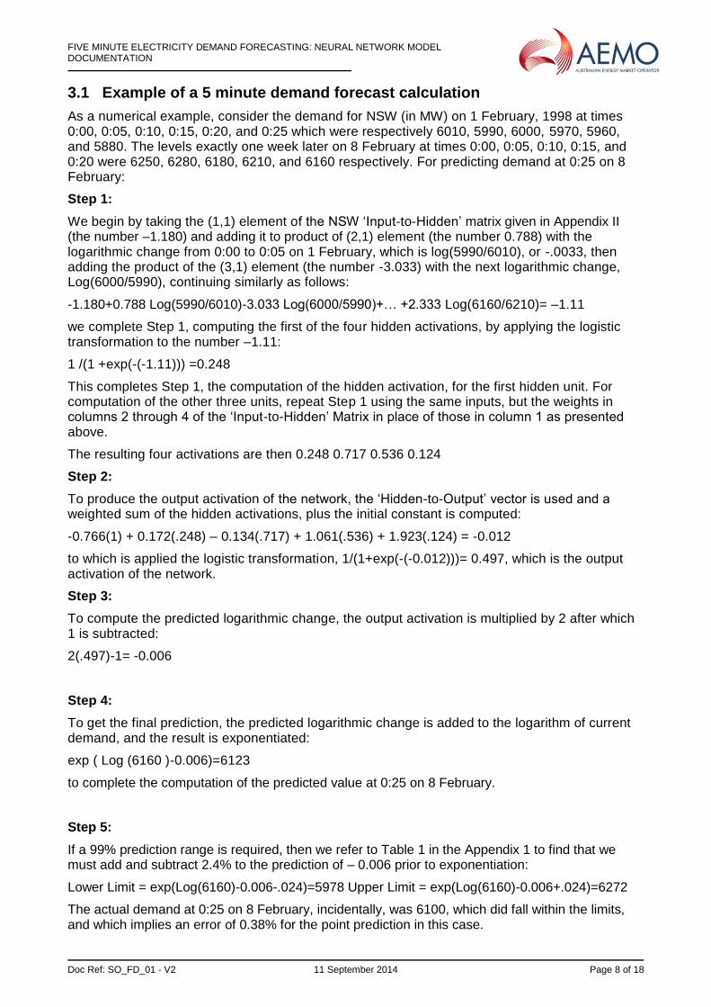
3.1 Example of a 5 minute demand forecast calculation

As a numerical example, consider the demand for NSW (in MW) on 1 February, 1998 at times 0:00, 0:05, 0:10, 0:15, 0:20, and 0:25 which were respectively 6010, 5990, 6000, 5970, 5960, and 5880. The levels exactly one week later on 8 February at times 0:00, 0:05, 0:10, 0:15, and 0:20 were 6250, 6280, 6180, 6210, and 6160 respectively. For predicting demand at 0:25 on 8 February:

Step 1:

We begin by taking the (1,1) element of the NSW ‘Input-to-Hidden’ matrix given in Appendix II (the number –1.180) and adding it to product of (2,1) element (the number 0.788) with the logarithmic change from 0:00 to 0:05 on 1 February, which is log(5990/6010), or -.0033, then adding the product of the (3,1) element (the number -3.033) with the next logarithmic change, Log(6000/5990), continuing similarly as follows:

-1.180+0.788 Log(5990/6010)-3.033 Log(6000/5990)+… +2.333 Log(6160/6210)= –1.11

we complete Step 1, computing the first of the four hidden activations, by applying the logistic transformation to the number –1.11:

1 /(1 +exp(-(-1.11))) =0.248

This completes Step 1, the computation of the hidden activation, for the first hidden unit. For computation of the other three units, repeat Step 1 using the same inputs, but the weights in columns 2 through 4 of the ‘Input-to-Hidden’ Matrix in place of those in column 1 as presented above.

The resulting four activations are then 0.248 0.717 0.536 0.124

Step 2:

To produce the output activation of the network, the ‘Hidden-to-Output’ vector is used and a weighted sum of the hidden activations, plus the initial constant is computed:

-0.766(1) + 0.172(.248) – 0.134(.717) + 1.061(.536) + 1.923(.124) = -0.012

to which is applied the logistic transformation, 1/(1+exp(-(-0.012)))= 0.497, which is the output activation of the network.

Step 3:

To compute the predicted logarithmic change, the output activation is multiplied by 2 after which 1 is subtracted:

2(.497)-1= -0.006

Step 4:

To get the final prediction, the predicted logarithmic change is added to the logarithm of current demand, and the result is exponentiated:

exp ( Log (6160 )-0.006)=6123

to complete the computation of the predicted value at 0:25 on 8 February.

Step 5:

If a 99% prediction range is required, then we refer to Table 1 in the Appendix 1 to find that we must add and subtract 2.4% to the prediction of – 0.006 prior to exponentiation:

Lower Limit = exp(Log(6160)-0.006-.024)=5978 Upper Limit = exp(Log(6160)-0.006+.024)=6272

The actual demand at 0:25 on 8 February, incidentally, was 6100, which did fall within the limits, and which implies an error of 0.38% for the point prediction in this case.

Five Minute Electricity Demand Forecasting: NEURAL NETWORK MODEL DOCUMENTATION


Appendix A Performance Summary of the Neural Network Model (Separate Fits, Various States)

Table 2: Performance Summary of the Neural Network Model (Separate Fits, Various States)

Region MSE %

(NAÏVE) BENCHMARK

MSE % (MODEL)

D % (REDUCT.)

CORR.(%) (MODEL)

MAPE %

(MODEL)

99%PI (MODEL)

NSW 0.0076 0.0048 37 61 0.52 (± )2.4

Victoria 0.0081 0.0061 25 50 0.58 (± )2.4

Qld. 0.0059 0.0039 33 58 0.57 (±)1.9

SA (est.) 0.0076* 0.0061* 20* 40* 0.58 (±)2.7*

* denotes extrapolated estimate for SA using NSW model



Appendix B Neural Network Matrix Weights for NSW, Queensland, Victoria, and South Australia

B.1 NSW (Pumping Station Load Removed) Perennial Model Data Basis: 5 Minute Demand May 1997 - May 1998

Input-to-Hidden Weight Matrix:

-1.18083652 .912479873 .168973233 -1.92511602

.787908442 -.280762392 -.0541686846 -.07762109

-3.03342919 -1.28836905 -.00341524871 -.161543795

-.805006387 -1.64200928 .662373364 .344925654

-2.24481232 -2.93899286 .409496988 1.99314546

-6.91548304 -.413204144 2.02470863 .843839487

1.899275 2.10931932 -.140064819 .648678667

1.67724099 -.0174202002 .0654530737 .752352854

3.34159312 -.498683481 -.384690811 1.15456333

2.33262311 1.10089596 -1.07629121 .839209192

Hidden-to-Output Weight Matrix:

-.766221613

.171686888

-.134112006

1.06132145

1.9234954

B.2 Queensland (Estimated Pumping Station Load Removed) Perennial Model Data Basis: 5 Minute Demand Jan-June 1998


.282659953 -1.49839082 -.537210429 .225580113

18.3616164 15.6772863 -71.7199107 -3.61382244

.138462075 -20.5994971 -30.1141459 8.57056617

19.6360212 -20.1458364 3.02027769 56.3019205

-4.66079932 8.23915687 41.4881728 55.5477574

-5.39211141 125.600091 107.21279 57.0884462



7.92197629 -9.82189813 -68.7600056 -9.66963952

-2.6961764 5.31600322 -36.6341694 -18.2310529

-14.2446113 15.6655053 11.4491824 -25.6384018

-17.957021 19.43863 1.34015688 -55.9344838

Hidden to Output Weight Matrix:

.0102750063

-.0633274108

.0281062647

-.0306966894

.0575090353

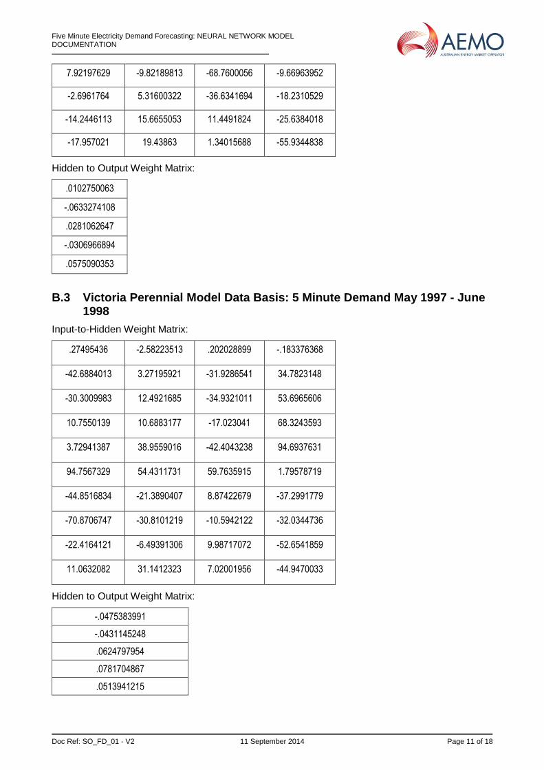
B.3 Victoria Perennial Model Data Basis: 5 Minute Demand May 1997 - June 1998


.27495436 -2.58223513 .202028899 -.183376368

-42.6884013 3.27195921 -31.9286541 34.7823148

-30.3009983 12.4921685 -34.9321011 53.6965606

10.7550139 10.6883177 -17.023041 68.3243593

3.72941387 38.9559016 -42.4043238 94.6937631

94.7567329 54.4311731 59.7635915 1.79578719

-44.8516834 -21.3890407 8.87422679 -37.2991779

-70.8706747 -30.8101219 -10.5942122 -32.0344736

-22.4164121 -6.49391306 9.98717072 -52.6541859

11.0632082 31.1412323 7.02001956 -44.9470033

Hidden to Output Weight Matrix:

-.0475383991

-.0431145248

.0624797954

.0781704867

.0513941215



B.4 South Australia (Pumping Station Load Removed) Perennial Model

Data Basis: Extrapolated from Average Half-Hourly Demand 1997 - 1998 5-Minute Demand, other states

Use weights for NSW Perennial model



Appendix C A Brief Introduction to Neural Network Modeling

While many modeling methods for real-world application have traditionally focused on ‘linear’ methods, such as linear regression, the past two decades have seen a dramatic increase in the application of nonlinear models in many areas. The increased efficiency which is required in the present era, accompanied by enormous technological improvement in computational capability and in data storage and processing, have meant that the development of more complex models for more complete, perhaps more subtle, modeling relationships has become and will continue to be a priority in many areas of application. Of these new nonlinear models, one family of generic models has begun to dominate, owing perhaps to both its ‘universality’ (networks’ ability to characterise virtually any desired functional relationship) and its appealing analogy to brain function.

In order to understand the basic motivation for Neural Network models (such as those being applied to the load prediction problem) it is helpful to describe a simple model of brain function. If one imagines a set of signals, perhaps emanating from an external stimulus, being propagated through axons and conveyed via synaptic connections of various strengths to neurons which ‘fire’, or activate, once a certain threshold is exceeded, and then the subsequent relay of these signals further to other neurons via axons and synaptic connections, continuing in a likewise manner, then a mathematical model for an input/output relationship is suggested.

Consider a system in which there exist signals which are regarded as inputs, which are relayed at various strengths or 'weights' to intermediate 'units', the signals for which are then relayed according to further weights, again and again until an output is reached. Then to alter the input/output relationship, one would merely need to change the values of the connection strengths, or weight-coefficient parameters, just as one might vary coefficients in linear regression. Following further, if the input/output relationship could be assessed or evaluated as to 'suitability' according to some numerical score, then the weights could be varied, randomly at first, then more pointedly, until a 'good' set of weight coefficients was achieved, as in the regression case, where ‘least-squares’ estimates are usually used. For understandable reasons, this process of adaptation of weight coefficients for suitability is called ‘learning’.

While linear models such as regression have existed and been applied successfully to many practical problems for some time for modeling input/output relationships, the introduction in Neural Network models of nonlinearity in the intermediate (often referred to as 'hidden') units leads to a qualitative shift in the modeling power of the system, in an analogous manner to the way in which the introduction of the diode as a nonlinear element into a standard electrical circuit was first seen to make possible the field of electronics when it was first introduced.

A mathematical property of Neural Networks, proved by Russian mathematicians in the 1960's, later clarified by work in the 1970's by mathematicians in the United States, is the Universal Approximation property of Neural Networks. In a word (under mild regularity conditions), this states that given any input/output relationship which exists for a finite number of examples, a Neural Network of sufficient complexity can approximate it arbitrarily well.

In practice, this means that for solving any given problem, instead of searching from within the potentially infinite number of possible functional families which could characterise the input/output relationship at hand, it suffices to consider the Neural Network family.

While this property has been understood for some time now, it is only with the recent development of high-speed of computing that it has any real meaning for useful real-world problems, as the Neural Network models needed for many or most nontrivial problems often require intense computation for fitting or 'learning'.

It is also perhaps worth noting that the image of the Neural Network as a 'superbrain' which might be implied from the brain analogy, should be avoided. Instead, perhaps the rather less glamorous image of the 'cockroach' is more appropriate; while cockroaches are not seen as being among the most insightful creatures on the planet, in a survival sense they indeed have arguably been among the most successful, having achieved this by reacting effectively to simple stimulus. As a prediction model, then, perhaps one might well do well to aim for a sort of 'cockroach efficiency'. This philosophy has guided the modeling for the present application.



Appendix D Schematic Diagram for Neural Network Load Prediction Model

Figure 1 Schematic Diagram for Neural Network Load Prediction Model

Inputs

Hidden Layer

Output



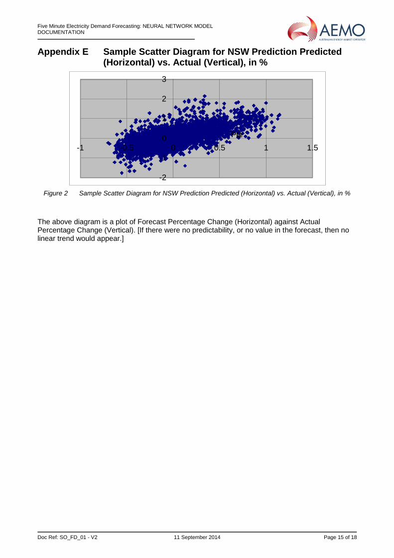
Appendix E Sample Scatter Diagram for NSW Prediction Predicted (Horizontal) vs. Actual (Vertical), in %

Figure 2 Sample Scatter Diagram for NSW Prediction Predicted (Horizontal) vs. Actual (Vertical), in %

The above diagram is a plot of Forecast Percentage Change (Horizontal) against Actual Percentage Change (Vertical). [If there were no predictability, or no value in the forecast, then no linear trend would appear.]

-2

-1

0

1

2

3

-1 -0.5 0 0.5 1 1.5

PDPre



Appendix F A Comment on Noise in 5-Minute Demand Forecasting

Previously, we have referred to the noise in the context of forecasting. This is in keeping with the traditional engineering approach of dividing a data series into two parts:

(i) Signal, a fixed predictable value, and

(ii) Noise, an inherently unpredictable random error. Generally, the objective in any forecasting problem is to remove as much of the Noise, or random error, as possible, so that the what remains is predominantly Signal.

For electricity demand forecasting, the nature of random error appears to be a combination of random bell-curve variables, plus extra occasional large ‘shocks’. The largest such shocks encountered in electricity demand in Australia appear to be due to large industrial loads that have a step change characteristic such as pumping station loads. Depending on one’s point of view, these changes may be regarded as either being random or non-random; while the amount of pumping station load is often predictable, the exact timing of it, being subject to substantial security protocol of varying duration, is not predictable unless it is communicated to the forecasting system, which is of course highly recommended.

In NSW and Victoria there appear to exist other sources of ‘shocks’, or large changes in demand, possibly due to smelting works, amounting to several per day. These do not appear to be present in the Queensland data, nor are they evident in the half-hourly South Australian data available. In other respects, the noise profiles in all regions appear to be similar, with regard to percentage changes in demand.



Appendix G A Note on Millennium Risk Exposure

To the extent that the Neural Network formulae are mathematical relationships from input to output, the only millennium risk involves the reliability of the system furnishing the input data to the model, or of the hardware used to implement the formulae; there is no inherent dependence of the forecasting formulae themselves on any Date functions.



Appendix H Summary of Statistical Formulae

H.1 Relative/Percentage Error

In prediction or forecasting, the relative error is defined as

(Predicted Value- Actual Value)/Actual Value

The percentage error is merely 100 times the relative error.

Mean Absolute Percentage Error (MAPE)

The absolute value (ABS) of a number is merely the distance of that number from zero (e.g. ABS(3)=3, ABS(-2)=2). These are computed by removing all minus (‘-’) signs. Hence, Absolute Percentage Error is the absolute value of the percentage error defined above. The Mean Absolute Percentage Error, then, is the average of these values for all predictions.

Mean Squared (Relative) Error (MSE)

The Mean Squared (Relative) Error is defined as the average of all of the squares of relative errors for all predictions.

Correlation

The Correlation is the expected cross-product between two standardised variables. [A standardised variable is a variable with its mean (or average) subtracted, afterwards scaled by dividing by standard deviation.] The correlation for the sample is defined as

r=1

n

x x

s

y y

s

i

x

i

y

( )( )

where x, y, sx and sy are the sample means and standard deviations of the two samples. A perfect negative relation is indicated by a correlation of -1, and a perfect positive relation by a correlation of +1, with a correlation of 0 corresponding to no linear relation. The square of correlation, R2 , is often referred to as the coefficient of determination, and may be interpreted as the proportion of variation in one variable (e.g., ‘Actual’ Load) which is predictable by a linear function of the other variable (e.g. ‘Predicted’ Load).

Date post:	21-Mar-2018
Category:	Documents
Upload:	vuongdang
View:	217 times
Download:	2 times

Five Minute Electricity Demand Forecasting: NEURAL NETWORK ... · PDF fileFIVE MINUTE...

Documents