Fixed-Bed Catalytic Reactors Copyright c 2016 by Nob Hill Publishing, LLC • In a fixed-bed reactor the catalyst pellets are held in place and do not move with respect to a fixed reference frame. • Material and energy balances are required for both the fluid, which occupies the interstitial region between catalyst particles, and the catalyst particles, in which the reactions occur. • The following figure presents several views of the fixed-bed reactor. The species production rates in the bulk fluid are essentially zero . That is the reason we are using a catalyst. 1
• In a fixed-bed reactor the catalyst pellets are held in place and do not movewith respect to a fixed reference frame.
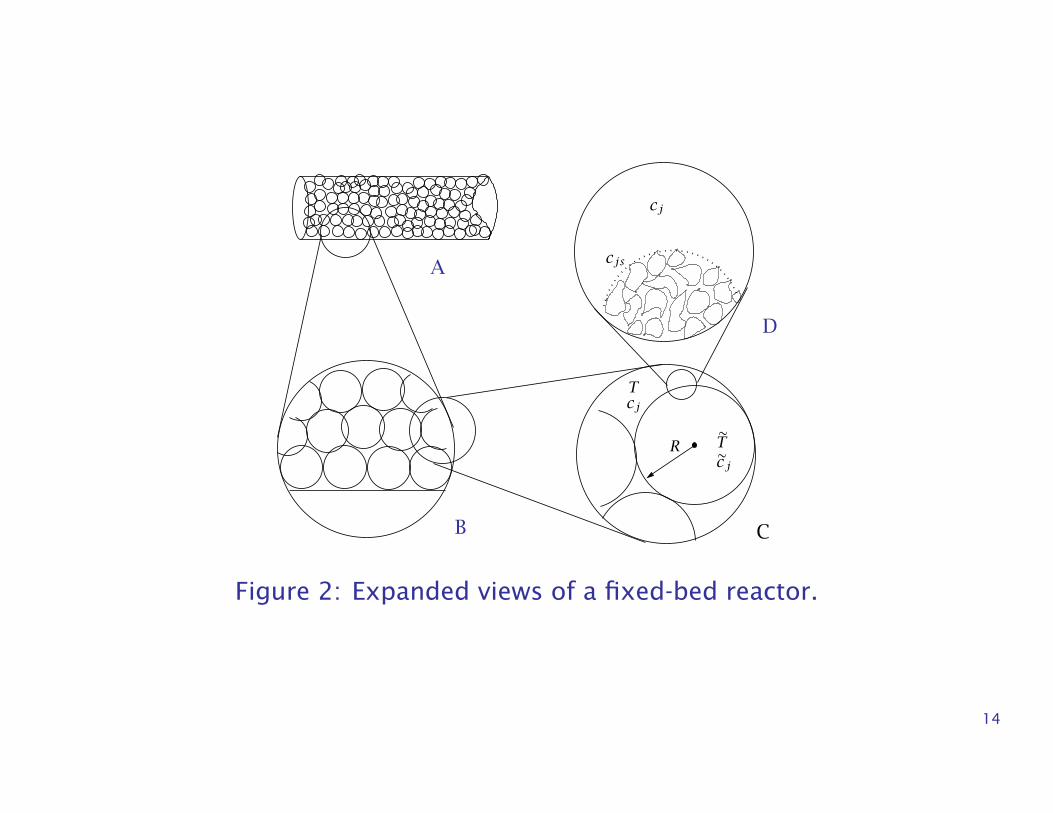
• Material and energy balances are required for both the fluid, which occupiesthe interstitial region between catalyst particles, and the catalyst particles, inwhich the reactions occur.
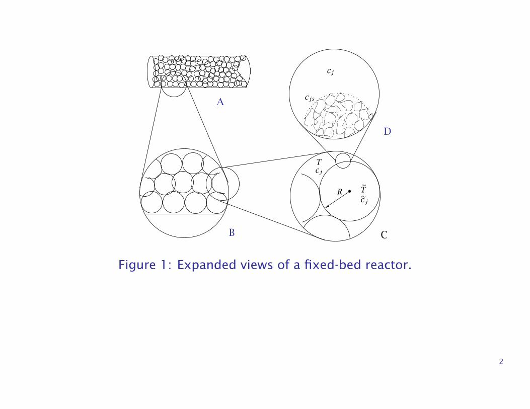
• The following figure presents several views of the fixed-bed reactor. Thespecies production rates in the bulk fluid are essentially zero. That is thereason we are using a catalyst.
1
B
A cjs
D
C
cj
cjT
R Tcj
Figure 1: Expanded views of a fixed-bed reactor.
2
The physical picture
• Essentially all reaction occurs within the catalyst particles. The fluid in contactwith the external surface of the catalyst pellet is denoted with subscript s.
• When we need to discuss both fluid and pellet concentrations and tempera-tures, we use a tilde on the variables within the catalyst pellet.
3
The steps to consider
During any catalytic reaction the following steps occur:
1. transport of reactants and energy from the bulk fluid up to the catalyst pelletexterior surface,
2. transport of reactants and energy from the external surface into the porouspellet,
3. adsorption, chemical reaction, and desorption of products at the catalyticsites,
4. transport of products from the catalyst interior to the external surface of thepellet, and
4
5. transport of products into the bulk fluid.
The coupling of transport processes with chemical reaction can lead to concen-tration and temperature gradients within the pellet, between the surface and thebulk, or both.
5
Some terminology and rate limiting steps
• Usually one or at most two of the five steps are rate limiting and act to influ-ence the overall rate of reaction in the pellet. The other steps are inherentlyfaster than the slow step(s) and can accommodate any change in the rate ofthe slow step.
• The system is intraparticle transport controlled if step 2 is the slow process(sometimes referred to as diffusion limited).
• For kinetic or reaction control, step 3 is the slowest process.
• Finally, if step 1 is the slowest process, the reaction is said to be externallytransport controlled.
6
Effective catalyst properties
• In this chapter, we model the system on the scale of Figure 1 C. The problemis solved for one pellet by averaging the microscopic processes that occuron the scale of level D over the volume of the pellet or over a solid surfacevolume element.
• This procedure requires an effective diffusion coefficient, Dj, to be identi-fied that contains information about the physical diffusion process and porestructure.
7
Catalyst Properties
• To make a catalytic process commercially viable, the number of sites per unitreactor volume should be such that the rate of product formation is on theorder of 1 mol/L·hour [12].
• In the case of metal catalysts, the metal is generally dispersed onto a high-area oxide such as alumina. Metal oxides also can be dispersed on a secondcarrier oxide such as vanadia supported on titania, or it can be made into ahigh-area oxide.
• These carrier oxides can have surface areas ranging from 0.05 m2/g to greaterthan 100 m2/g.
• The carrier oxides generally are pressed into shapes or extruded into pellets.
8
Catalyst Properties
• The following shapes are frequently used in applications:
– 20–100 µm diameter spheres for fluidized-bed reactors– 0.3–0.7 cm diameter spheres for fixed-bed reactors– 0.3–1.3 cm diameter cylinders with a length-to-diameter ratio of 3–4– up to 2.5 cm diameter hollow cylinders or rings.
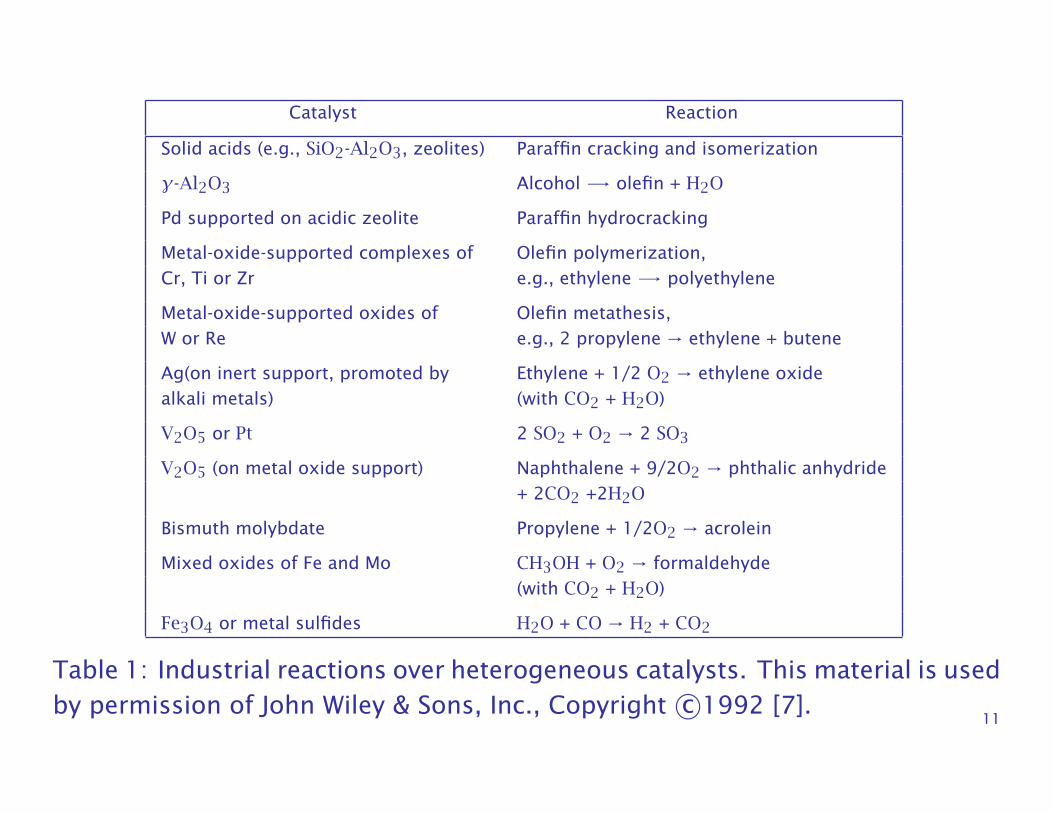
• Table 1 lists some of the important commercial catalysts and their uses [7].
9
Catalyst Reaction
Metals (e.g., Ni, Pd, Pt, as powders C C bond hydrogenation, e.g.,or on supports) or metal oxides olefin + H2 -→ paraffin(e.g., Cr2O3)
Metals (e.g., Cu, Ni, Pt) C O bond hydrogenation, e.g.,acetone + H2 -→ isopropanol
Metal (e.g., Pd, Pt) Complete oxidation of hydrocarbons,oxidation of CO
Fe (supported and promoted with 3H2 + N2 -→ 2NH3alkali metals)
Ni CO + 3H2 -→ CH4 + H2O (methanation)
Fe or Co (supported and promoted CO + H2 -→ paraffins + olefins + H2Owith alkali metals) + CO2 (+ other oxygen-containing organic
compounds) (Fischer-Tropsch reaction)
Cu (supported on ZnO, with other CO + 2H2 -→ CH3OHcomponents, e.g., Al2O3)
Re + Pt (supported on η-Al2O3 or Paraffin dehydrogenation, isomerizationγ-Al2O3 promoted with chloride) and dehydrocyclization
10
Catalyst Reaction
Solid acids (e.g., SiO2-Al2O3, zeolites) Paraffin cracking and isomerization
γ-Al2O3 Alcohol -→ olefin + H2O
Pd supported on acidic zeolite Paraffin hydrocracking
Metal-oxide-supported complexes of Olefin polymerization,Cr, Ti or Zr e.g., ethylene -→ polyethylene
Metal-oxide-supported oxides of Olefin metathesis,W or Re e.g., 2 propylene → ethylene + butene
Ag(on inert support, promoted by Ethylene + 1/2 O2 → ethylene oxidealkali metals) (with CO2 + H2O)
V2O5 or Pt 2 SO2 + O2 → 2 SO3
V2O5 (on metal oxide support) Naphthalene + 9/2O2 → phthalic anhydride+ 2CO2 +2H2O
Bismuth molybdate Propylene + 1/2O2 → acrolein
Mixed oxides of Fe and Mo CH3OH + O2 → formaldehyde(with CO2 + H2O)
• Figure 1 D of shows a schematic representation of the cross section of a singlepellet.
• The solid density is denoted ρs.
• The pellet volume consists of both void and solid. The pellet void fraction (orporosity) is denoted by ε and
ε = ρpVgin which ρp is the effective particle or pellet density and Vg is the pore volume.
• The pore structure is a strong function of the preparation method, and cata-lysts can have pore volumes (Vg) ranging from 0.1–1 cm3/g pellet.
12
Pore properties
• The pores can be the same size or there can be a bimodal distribution withpores of two different sizes, a large size to facilitate transport and a smallsize to contain the active catalyst sites.
• Pore sizes can be as small as molecular dimensions (several Angstroms) oras large as several millimeters.
• Total catalyst area is generally determined using a physically adsorbedspecies, such as N2. The procedure was developed in the 1930s by Brunauer,Emmett and and Teller [5], and the isotherm they developed is referred to asthe BET isotherm.
13
B
A cjs
D
C
cj
cjT
R Tcj
Figure 2: Expanded views of a fixed-bed reactor.
14
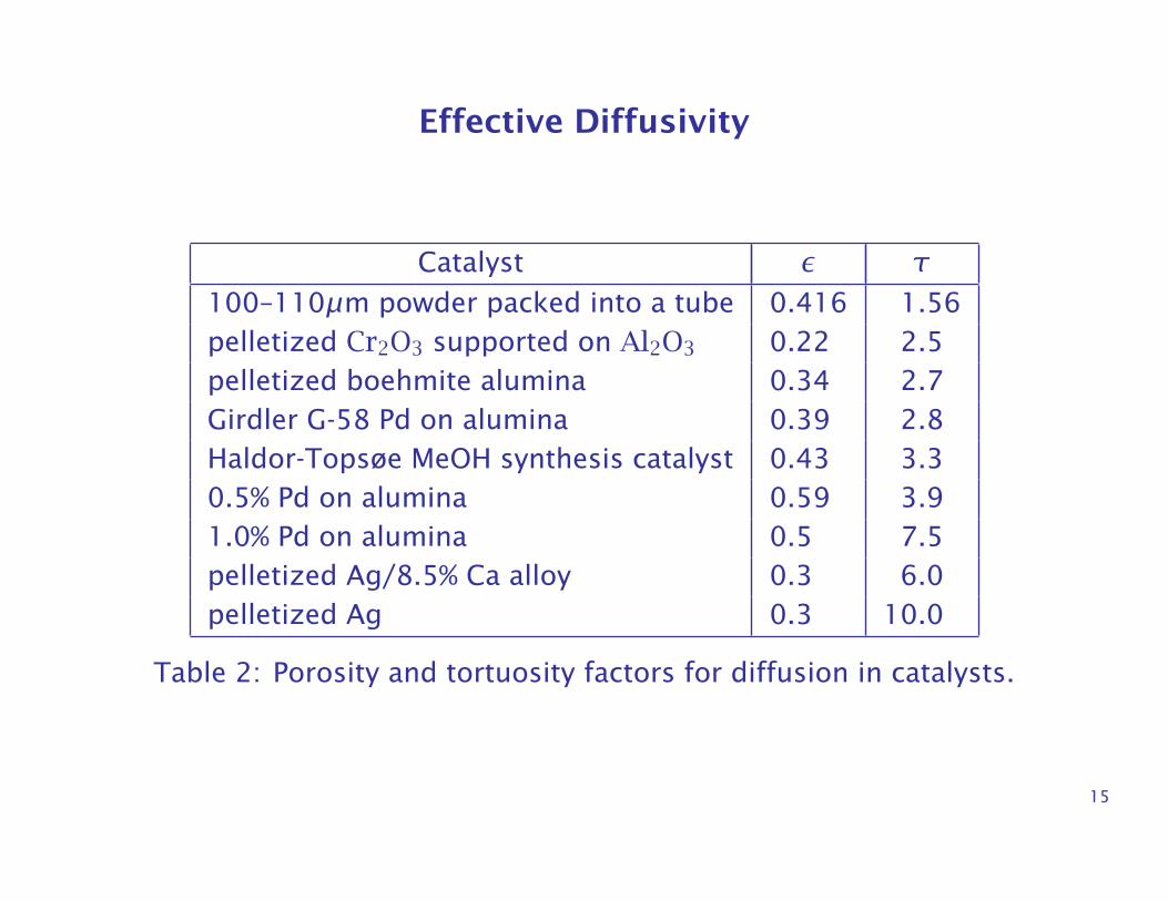
Effective Diffusivity
Catalyst ε τ100–110µm powder packed into a tube 0.416 1.56pelletized Cr2O3 supported on Al2O3 0.22 2.5pelletized boehmite alumina 0.34 2.7Girdler G-58 Pd on alumina 0.39 2.8Haldor-Topsøe MeOH synthesis catalyst 0.43 3.30.5% Pd on alumina 0.59 3.91.0% Pd on alumina 0.5 7.5pelletized Ag/8.5% Ca alloy 0.3 6.0pelletized Ag 0.3 10.0
Table 2: Porosity and tortuosity factors for diffusion in catalysts.
15
The General Balances in the Catalyst Particle
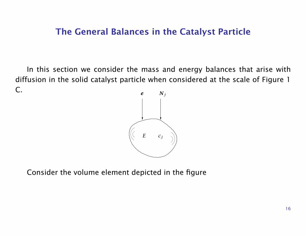
In this section we consider the mass and energy balances that arise withdiffusion in the solid catalyst particle when considered at the scale of Figure 1C. e Nj
E cj
Consider the volume element depicted in the figure
16
Balances
Assume a fixed laboratory coordinate system in which the velocities are de-fined and let vj be the velocity of species j giving rise to molar flux Nj
Nj = cjvj, j = 1,2, . . . , ns
Let E be the total energy within the volume element and e be the flux of totalenergy through the bounding surface due to all mechanisms of transport. Theconservation of mass and energy for the volume element implies
∂cj∂t= −∇ ·Nj + Rj, j = 1,2, . . . , ns (1)
∂E∂t= −∇ · e (2)
in which Rj accounts for the production of species j due to chemical reaction.
17
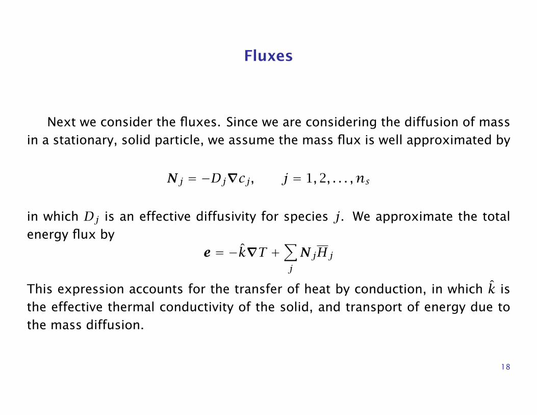
Fluxes
Next we consider the fluxes. Since we are considering the diffusion of massin a stationary, solid particle, we assume the mass flux is well approximated by
Nj = −Dj∇cj, j = 1,2, . . . , ns
in which Dj is an effective diffusivity for species j. We approximate the totalenergy flux by
e = −k∇T +∑jNjHj
This expression accounts for the transfer of heat by conduction, in which k isthe effective thermal conductivity of the solid, and transport of energy due tothe mass diffusion.
18
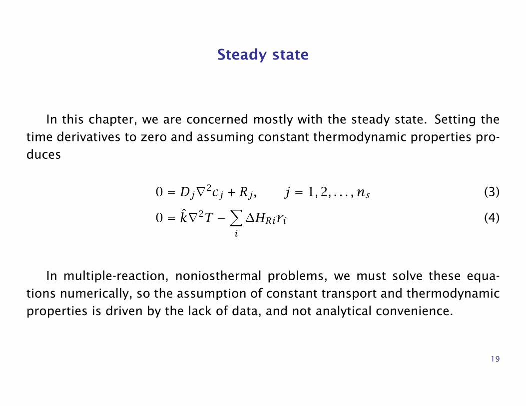
Steady state
In this chapter, we are concerned mostly with the steady state. Setting thetime derivatives to zero and assuming constant thermodynamic properties pro-duces
0 = Dj∇2cj + Rj, j = 1,2, . . . , ns (3)
0 = k∇2T −∑i∆HRiri (4)
In multiple-reaction, noniosthermal problems, we must solve these equa-tions numerically, so the assumption of constant transport and thermodynamicproperties is driven by the lack of data, and not analytical convenience.
19
Single Reaction in an Isothermal Particle
• We start with the simplest cases and steadily remove restrictions and increasethe generality. We consider in this section a single reaction taking place inan isothermal particle.
• First case: the spherical particle, first-order reaction, without external mass-transfer resistance.
• Next we consider other catalyst shapes, then other reaction orders, and thenother kinetic expressions such as the Hougen-Watson kinetics of Chapter 5.
• We end the section by considering the effects of finite external mass transfer.
20
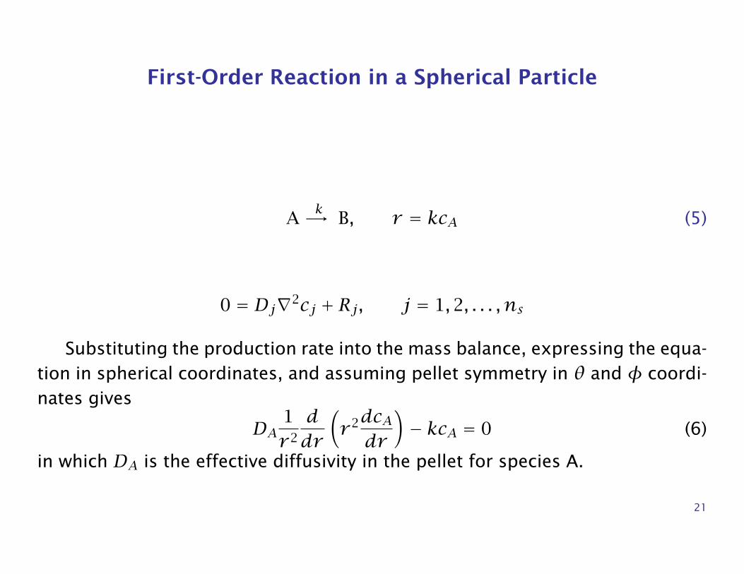
First-Order Reaction in a Spherical Particle
Ak-→ B, r = kcA (5)
0 = Dj∇2cj + Rj, j = 1,2, . . . , ns
Substituting the production rate into the mass balance, expressing the equa-tion in spherical coordinates, and assuming pellet symmetry in θ and φ coordi-nates gives
DA1r 2
ddr
(r 2dcAdr
)− kcA = 0 (6)
in which DA is the effective diffusivity in the pellet for species A.
21
Units of rate constant
As written here, the first-order rate constant k has units of inverse time.
Be aware that the units for a heterogeneous reaction rate constant are some-times expressed per mass or per area of catalyst.
In these cases, the reaction rate expression includes the conversion factors,catalyst density or catalyst area, as illustrated in Example 7.1.
22
Boundary Conditions
• We require two boundary conditions for Equation 6.
• In this section we assume the concentration at the outer boundary of thepellet, cAs, is known
• The symmetry of the spherical pellet implies the vanishing of the derivativeat the center of the pellet.
• Therefore the two boundary conditions for Equation 6 are
cA = cAs, r = RdcAdr
= 0 r = 0
23
Dimensionless form
At this point we can obtain better insight by converting the problem intodimensionless form. Equation 6 has two dimensional quantities, length andconcentration. We might naturally choose the sphere radius R as the lengthscale, but we will find that a better choice is to use the pellet’s volume-to-surfaceratio. For the sphere, this characteristic length is
a = VpSp=
43πR
3
4πR2= R
3(7)
The only concentration appearing in the problem is the surface concentrationin the boundary condition, so we use that quantity to nondimensionalize theconcentration
r = ra, c = cA
cAs
24
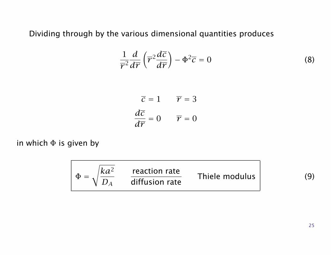
Dividing through by the various dimensional quantities produces
1
r 2
ddr
(r 2dcdr
)− Φ2c = 0 (8)
c = 1 r = 3
dcdr= 0 r = 0
in which Φ is given by
Φ =√ka2
DAreaction ratediffusion rate
Thiele modulus (9)
25
Thiele Modulus — Φ
The single dimensionless group appearing in the model is referred to as theThiele number or Thiele modulus in recognition of Thiele’s pioneering contribu-tion in this area [11].1 The Thiele modulus quantifies the ratio of the reactionrate to the diffusion rate in the pellet.
1In his original paper, Thiele used the term modulus to emphasize that this then unnamed dimensionlessgroup was positive. Later when Thiele’s name was assigned to this dimensionless group, the term modulus wasretained. Thiele number would seem a better choice, but the term Thiele modulus has become entrenched.
26
Solving the model
We now wish to solve Equation 8 with the given boundary conditions. Becausethe reaction is first order, the model is linear and we can derive an analyticalsolution.
It is often convenient in spherical coordinates to consider the variable trans-formation
c(r) = u(r)r
(10)
Substituting this relation into Equation 8 provides a simpler differential equa-tion for u(r),
d2udr 2 − Φ
2u = 0 (11)
27
with the transformed boundary conditions
u = 3 r = 3
u = 0 r = 0
The boundary condition u = 0 at r = 0 ensures that c is finite at the centerof the pellet.
28
General solution – hyperbolic functions
The solution to Equation 11 is
u(r) = c1 coshΦr + c2 sinhΦr (12)
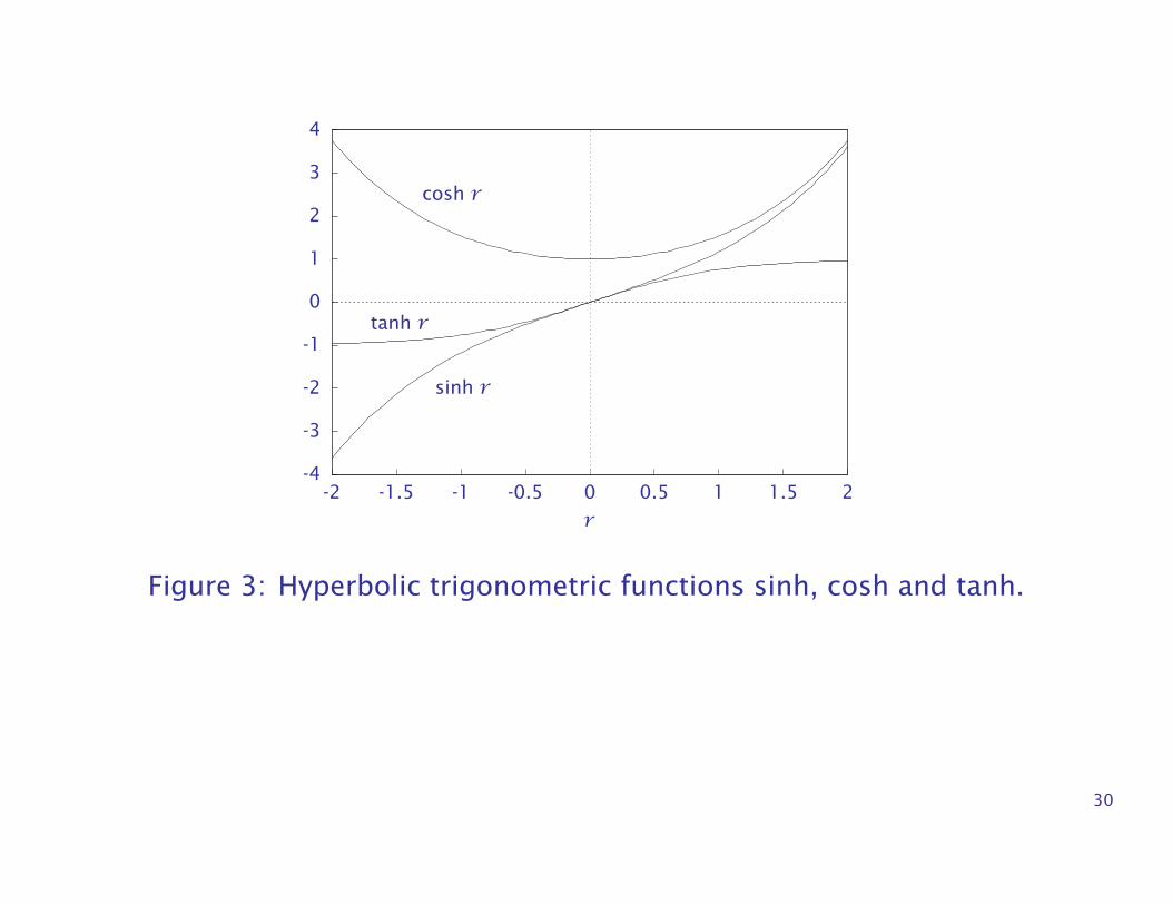
This solution is analogous to the sine and cosine solutions if one replaces thenegative sign with a positive sign in Equation 11. These functions are shown inFigure 3.
29
-4
-3
-2
-1
0
1
2
3
4
-2 -1.5 -1 -0.5 0 0.5 1 1.5 2
sinh r
cosh r
tanh r
r
Figure 3: Hyperbolic trigonometric functions sinh, cosh and tanh.
30
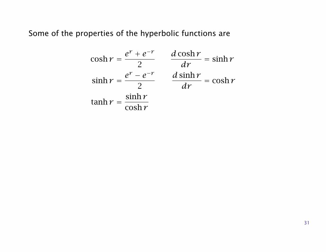
Some of the properties of the hyperbolic functions are
cosh r = er + e−r
2d cosh rdr
= sinh r
sinh r = er − e−r
2d sinh rdr
= cosh r
tanh r = sinh rcosh r
31
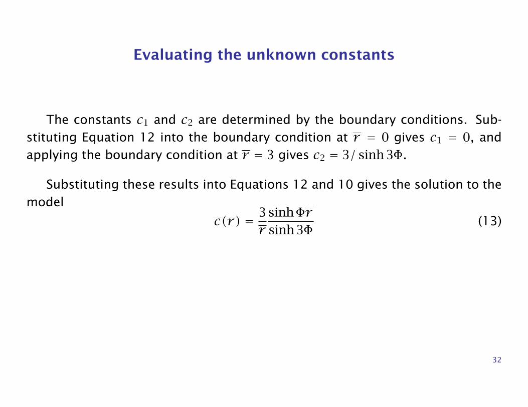
Evaluating the unknown constants
The constants c1 and c2 are determined by the boundary conditions. Sub-stituting Equation 12 into the boundary condition at r = 0 gives c1 = 0, andapplying the boundary condition at r = 3 gives c2 = 3/ sinh 3Φ.
Substituting these results into Equations 12 and 10 gives the solution to themodel
c(r) = 3r
sinhΦrsinh 3Φ
(13)
32
Every picture tells a story
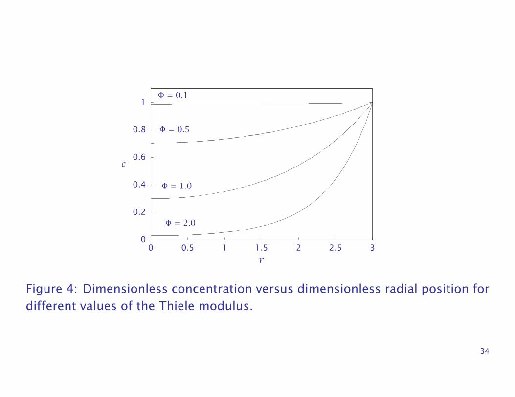
Figure 4 displays this solution for various values of the Thiele modulus.
Note for small values of Thiele modulus, the reaction rate is small comparedto the diffusion rate, and the pellet concentration becomes nearly uniform. Forlarge values of Thiele modulus, the reaction rate is large compared to the diffu-sion rate, and the reactant is converted to product before it can penetrate veryfar into the pellet.
33
0
0.2
0.4
0.6
0.8
1
0 0.5 1 1.5 2 2.5 3
Φ = 0.1
Φ = 0.5
Φ = 1.0
Φ = 2.0
c
r
Figure 4: Dimensionless concentration versus dimensionless radial position fordifferent values of the Thiele modulus.
34
Pellet total production rate
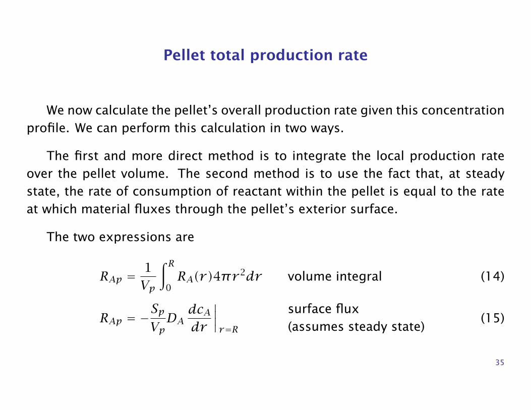
We now calculate the pellet’s overall production rate given this concentrationprofile. We can perform this calculation in two ways.
The first and more direct method is to integrate the local production rateover the pellet volume. The second method is to use the fact that, at steadystate, the rate of consumption of reactant within the pellet is equal to the rateat which material fluxes through the pellet’s exterior surface.
The two expressions are
RAp =1Vp
∫ R0RA(r)4πr 2dr volume integral (14)
RAp = −SpVpDAdcAdr
∣∣∣∣r=R
surface flux(assumes steady state)
(15)
35
in which the local production rate is given by RA(r) = −kcA(r).
We use the direct method here and leave the other method as an exercise.
36
Some integration
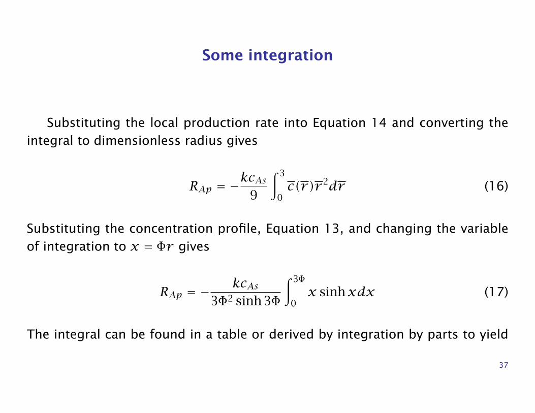
Substituting the local production rate into Equation 14 and converting theintegral to dimensionless radius gives
RAp = −kcAs
9
∫ 3
0c(r)r 2dr (16)
Substituting the concentration profile, Equation 13, and changing the variableof integration to x = Φr gives
RAp = −kcAs
3Φ2 sinh 3Φ
∫ 3Φ
0x sinhxdx (17)
The integral can be found in a table or derived by integration by parts to yield
37
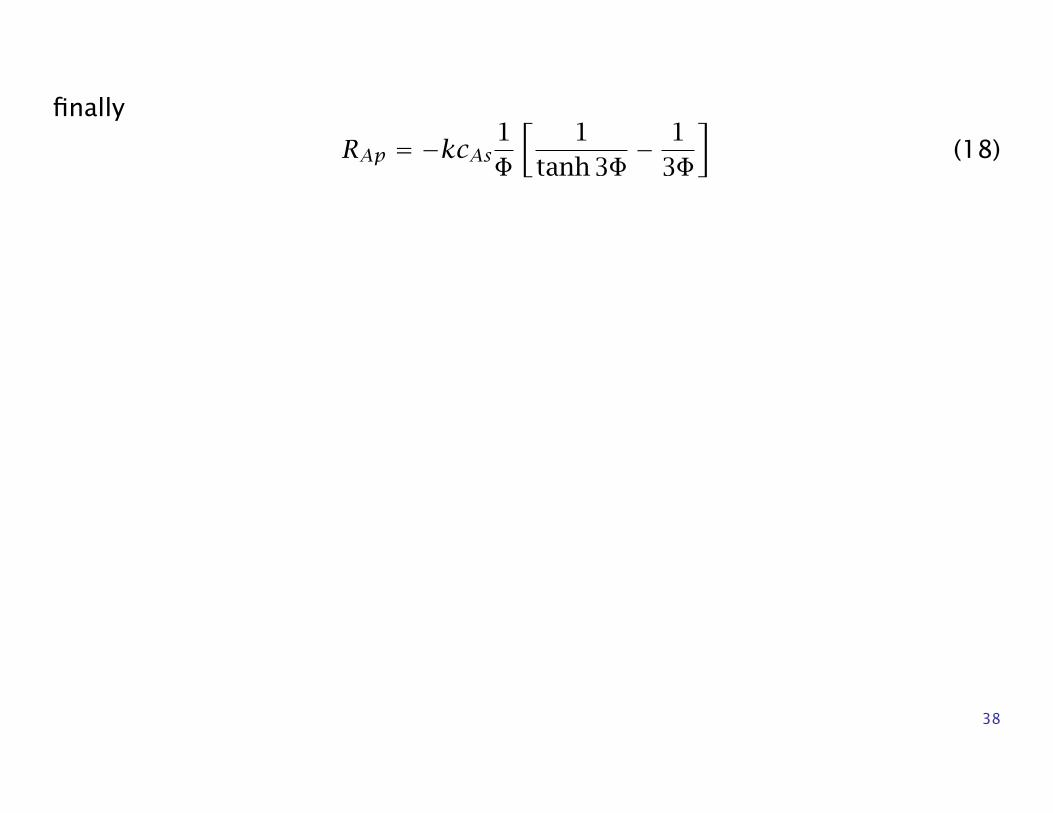
finally
RAp = −kcAs1Φ
[1
tanh 3Φ− 1
3Φ
](18)
38
Effectiveness factor η
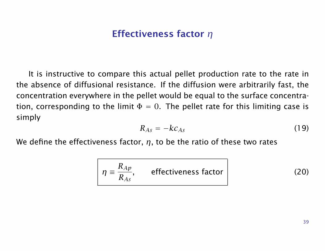
It is instructive to compare this actual pellet production rate to the rate inthe absence of diffusional resistance. If the diffusion were arbitrarily fast, theconcentration everywhere in the pellet would be equal to the surface concentra-tion, corresponding to the limit Φ = 0. The pellet rate for this limiting case issimply
RAs = −kcAs (19)
We define the effectiveness factor, η, to be the ratio of these two rates
η ≡ RApRAs
, effectiveness factor (20)
39
Effectiveness factor is the pellet production rate
The effectiveness factor is a dimensionless pellet production rate that mea-sures how effectively the catalyst is being used.
For η near unity, the entire volume of the pellet is reacting at the same highrate because the reactant is able to diffuse quickly through the pellet.
For η near zero, the pellet reacts at a low rate. The reactant is unable topenetrate significantly into the interior of the pellet and the reaction rate issmall in a large portion of the pellet volume.
The pellet’s diffusional resistance is large and this resistance lowers the over-all reaction rate.
40
Effectiveness factor for our problem
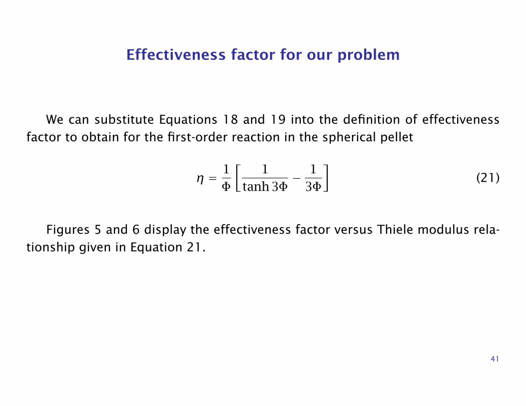
We can substitute Equations 18 and 19 into the definition of effectivenessfactor to obtain for the first-order reaction in the spherical pellet
η = 1Φ
[1
tanh 3Φ− 1
3Φ
](21)
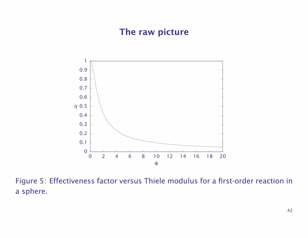
Figures 5 and 6 display the effectiveness factor versus Thiele modulus rela-tionship given in Equation 21.
41
The raw picture
0
0.1
0.2
0.3
0.4
0.5
0.6
0.7
0.8
0.9
1
0 2 4 6 8 10 12 14 16 18 20
η
Φ
Figure 5: Effectiveness factor versus Thiele modulus for a first-order reaction ina sphere.
42
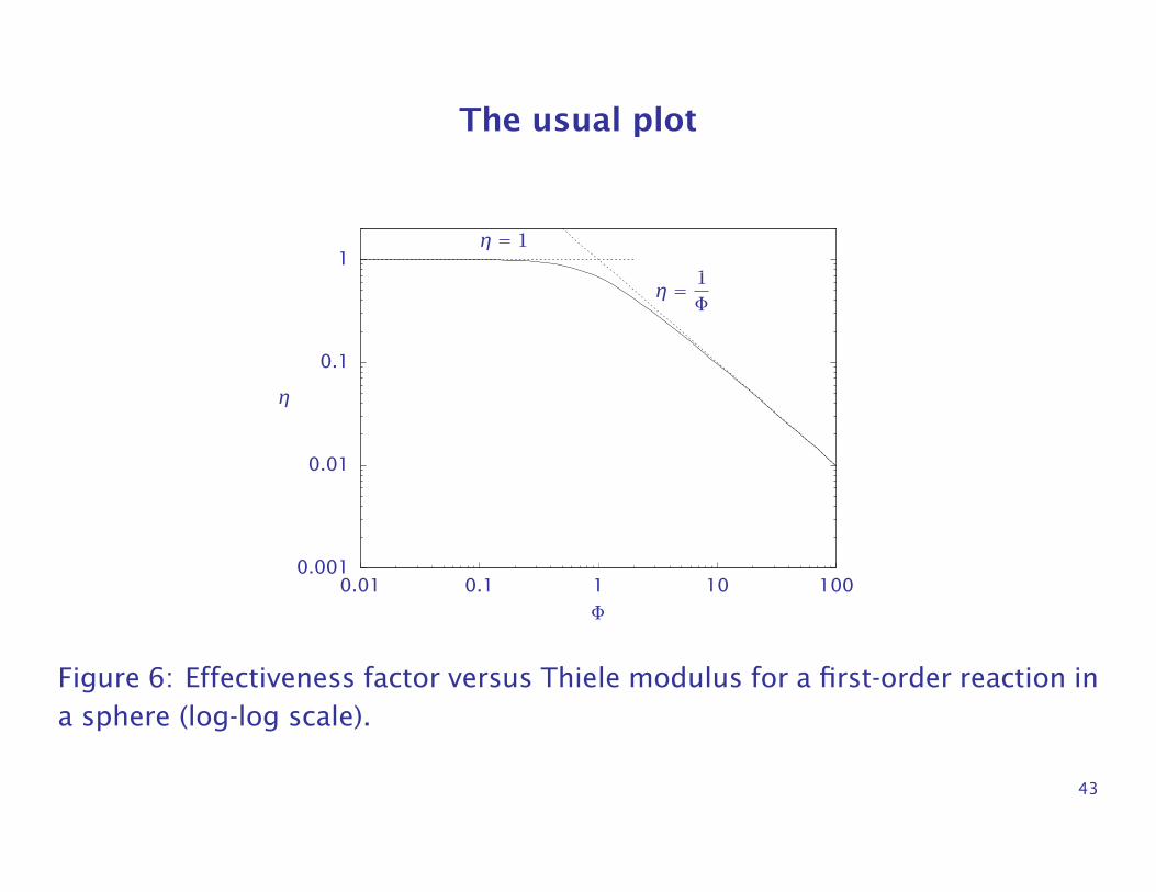
The usual plot
0.001
0.01
0.1
1
0.01 0.1 1 10 100
η = 1Φ
η
η = 1
Φ
Figure 6: Effectiveness factor versus Thiele modulus for a first-order reaction ina sphere (log-log scale).
43
The log-log scale in Figure 6 is particularly useful, and we see the two asymp-totic limits of Equation 21.
At small Φ, η ≈ 1, and at large Φ, η ≈ 1/Φ.
Figure 6 shows that the asymptote η = 1/Φ is an excellent approximationfor the spherical pellet for Φ ≥ 10.
For large values of the Thiele modulus, the rate of reaction is much greaterthan the rate of diffusion, the effectiveness factor is much less than unity, andwe say the pellet is diffusion limited.
Conversely, when the diffusion rate is much larger than the reaction rate, theeffectiveness factor is near unity, and we say the pellet is reaction limited.
44
Example — Using the Thiele modulus and effectiveness factor
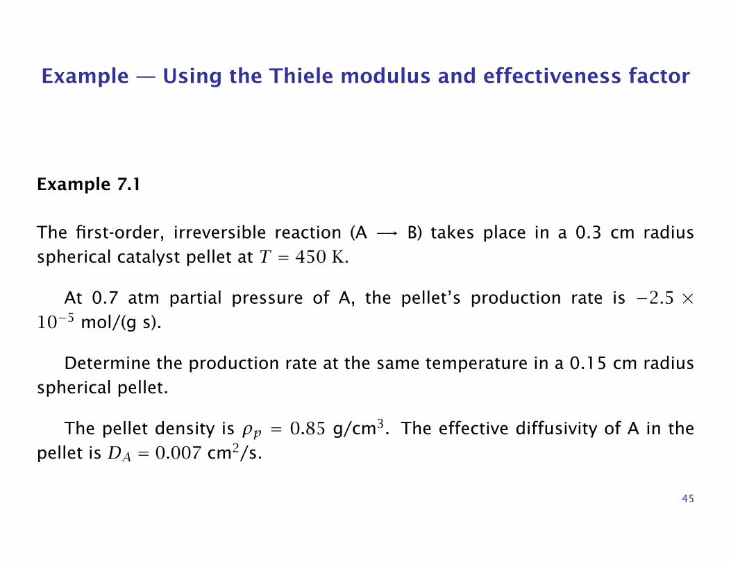
Example 7.1
The first-order, irreversible reaction (A -→ B) takes place in a 0.3 cm radiusspherical catalyst pellet at T = 450 K.
At 0.7 atm partial pressure of A, the pellet’s production rate is −2.5 ×10⁻⁵ mol/(g s).
Determine the production rate at the same temperature in a 0.15 cm radiusspherical pellet.
The pellet density is ρp = 0.85 g/cm3. The effective diffusivity of A in thepellet is DA = 0.007 cm2/s.
45
Solution
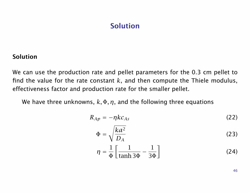
Solution
We can use the production rate and pellet parameters for the 0.3 cm pellet tofind the value for the rate constant k, and then compute the Thiele modulus,effectiveness factor and production rate for the smaller pellet.
We have three unknowns, k,Φ, η, and the following three equations
RAp = −ηkcAs (22)
Φ =√ka2
DA(23)
η = 1Φ
[1
tanh 3Φ− 1
3Φ
](24)
46
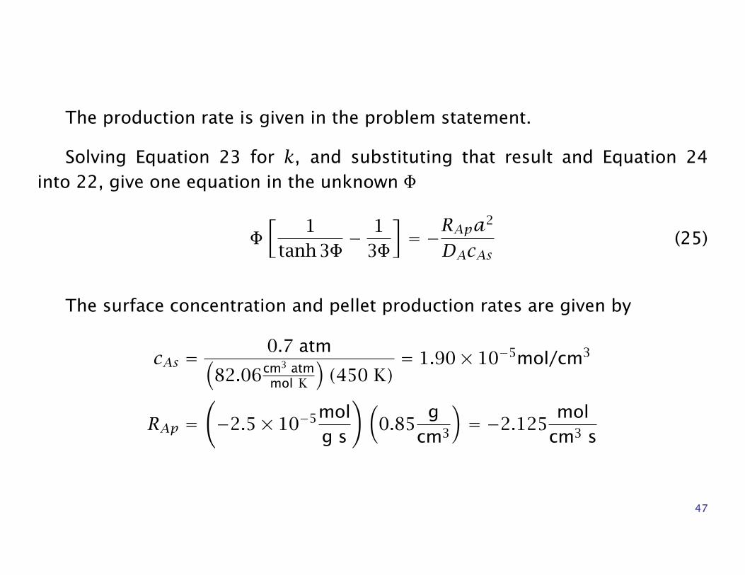
The production rate is given in the problem statement.
Solving Equation 23 for k, and substituting that result and Equation 24into 22, give one equation in the unknown Φ
Φ[
1tanh 3Φ
− 13Φ
]= −RApa
2
DAcAs(25)
The surface concentration and pellet production rates are given by
cAs =0.7 atm(
82.06cm3 atmmol K
)(450 K)
= 1.90× 10⁻⁵mol/cm3
RAp =(−2.5× 10⁻⁵mol
g s
)(0.85
gcm3
)= −2.125
molcm3 s
47
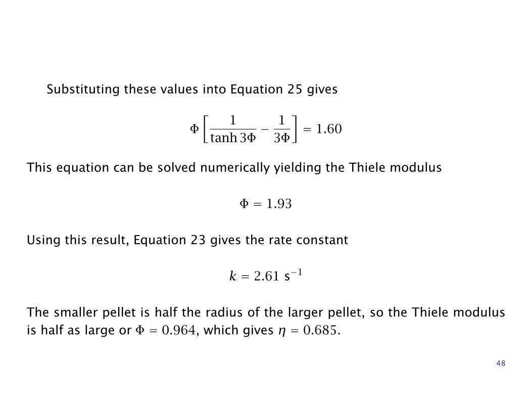
Substituting these values into Equation 25 gives
Φ[
1tanh 3Φ
− 13Φ
]= 1.60
This equation can be solved numerically yielding the Thiele modulus
Φ = 1.93
Using this result, Equation 23 gives the rate constant
k = 2.61 s−1
The smaller pellet is half the radius of the larger pellet, so the Thiele modulusis half as large or Φ = 0.964, which gives η = 0.685.
48
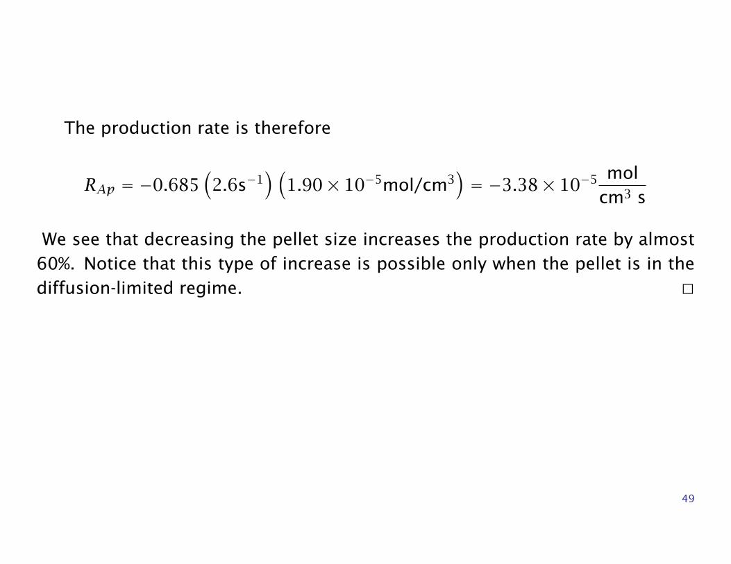
The production rate is therefore
RAp = −0.685(
2.6s−1)(
1.90× 10⁻⁵mol/cm3)= −3.38× 10⁻⁵ mol
cm3 s
We see that decreasing the pellet size increases the production rate by almost60%. Notice that this type of increase is possible only when the pellet is in thediffusion-limited regime.
49
Other Catalyst Shapes: Cylinders and Slabs
Here we consider the cylinder and slab geometries in addition to the spherecovered in the previous section.
To have a simple analytical solution, we must neglect the end effects.
We therefore consider in addition to the sphere of radius Rs, the semi-infinitecylinder of radius Rc, and the semi-infinite slab of thickness 2L, depicted inFigure 7.
50
Rs
Rc
L
a = Rc/2
a = L
a = Rs/3
Figure 7: Characteristic length a for sphere, semi-infinite cylinder and semi-in-finite slab.
51
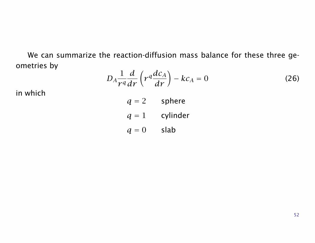
We can summarize the reaction-diffusion mass balance for these three ge-ometries by
DA1rqddr
(rqdcAdr
)− kcA = 0 (26)
in whichq = 2 sphere
q = 1 cylinder
q = 0 slab
52
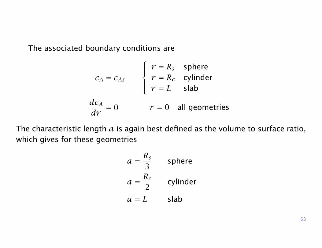
The associated boundary conditions are
cA = cAs
r = Rs spherer = Rc cylinderr = L slab
dcAdr
= 0 r = 0 all geometries
The characteristic length a is again best defined as the volume-to-surface ratio,which gives for these geometries
a = Rs3
sphere
a = Rc2
cylinder
a = L slab
53
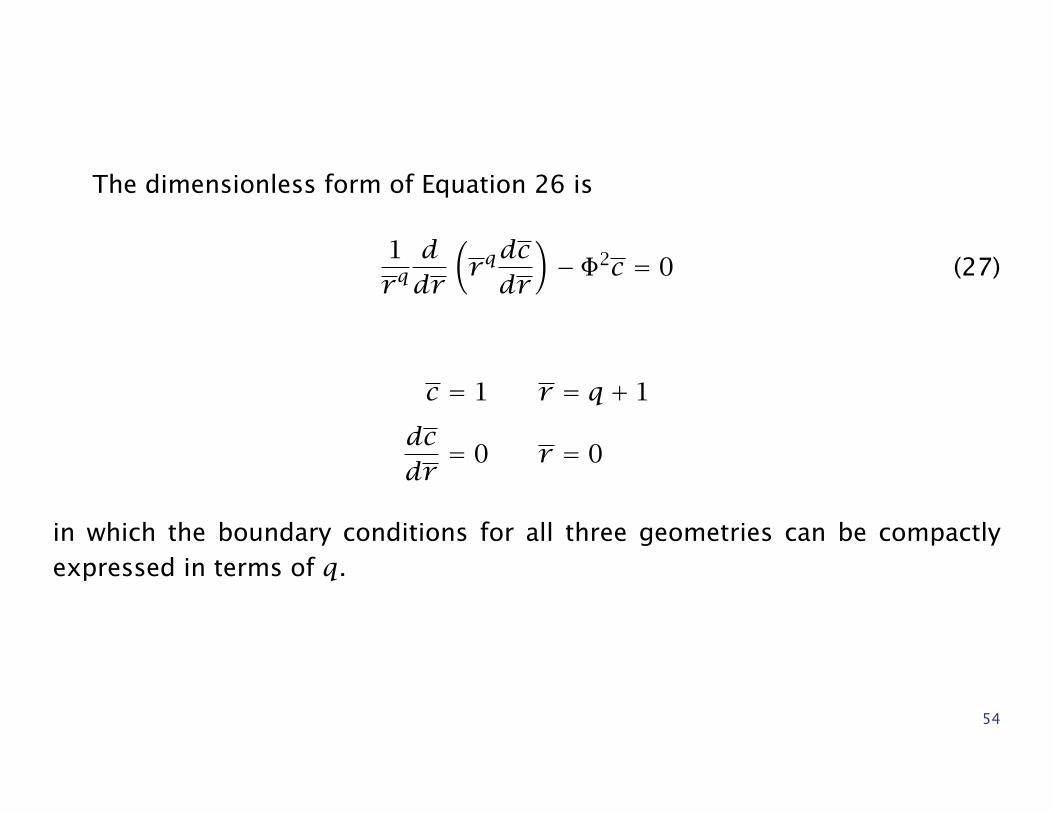
The dimensionless form of Equation 26 is
1rqddr
(rqdcdr
)− Φ2c = 0 (27)
c = 1 r = q + 1
dcdr= 0 r = 0
in which the boundary conditions for all three geometries can be compactlyexpressed in terms of q.
54
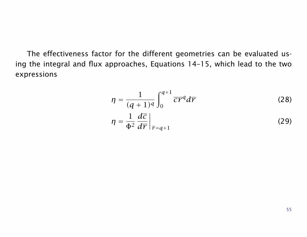
The effectiveness factor for the different geometries can be evaluated us-ing the integral and flux approaches, Equations 14–15, which lead to the twoexpressions
η = 1(q + 1)q
∫ q+1
0crqdr (28)
η = 1Φ2
dcdr
∣∣∣∣r=q+1
(29)
55
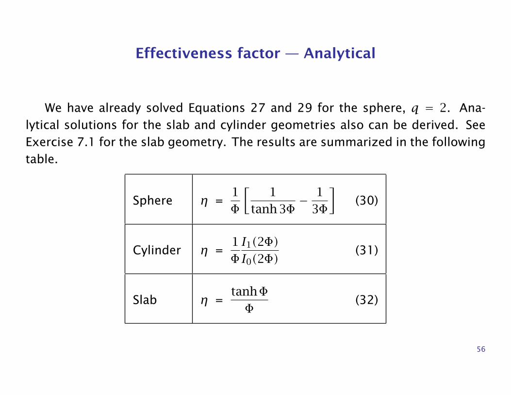
Effectiveness factor — Analytical
We have already solved Equations 27 and 29 for the sphere, q = 2. Ana-lytical solutions for the slab and cylinder geometries also can be derived. SeeExercise 7.1 for the slab geometry. The results are summarized in the followingtable.
Sphere η =1Φ
[1
tanh 3Φ− 1
3Φ
](30)
Cylinder η =1ΦI1(2Φ)I0(2Φ)
(31)
Slab η =tanhΦΦ
(32)
56
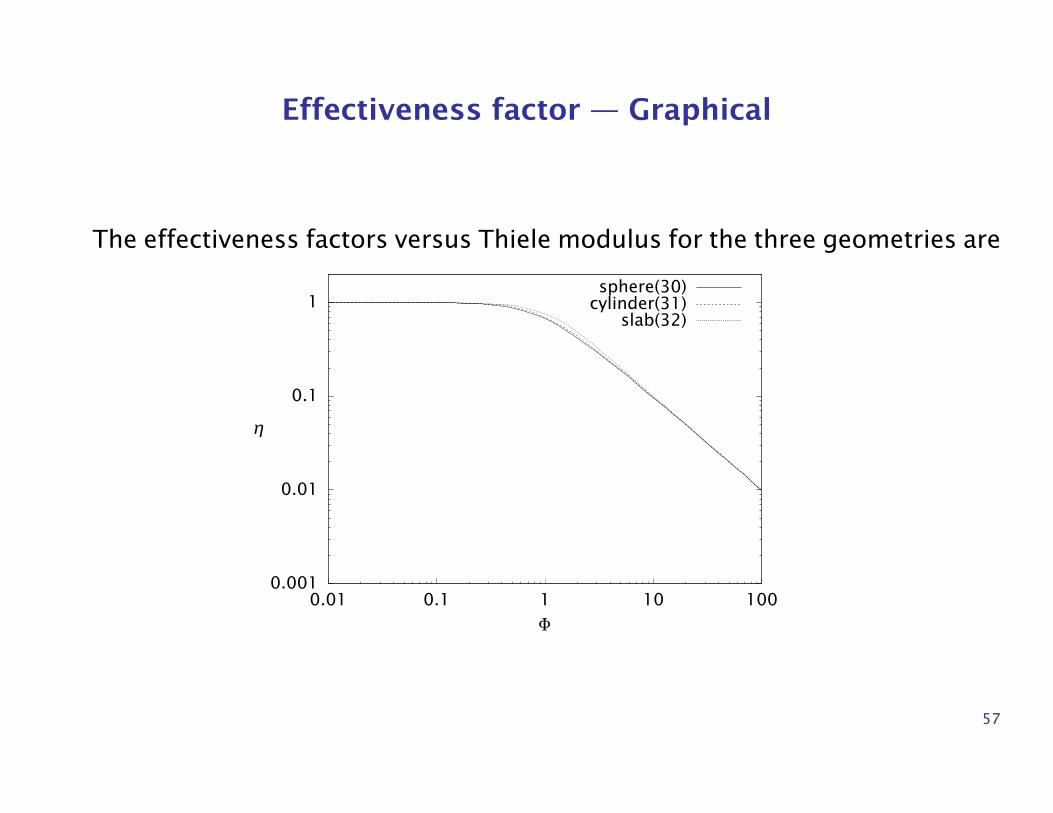
Effectiveness factor — Graphical
The effectiveness factors versus Thiele modulus for the three geometries are
0.001
0.01
0.1
1
0.01 0.1 1 10 100
η
Φ
sphere(30)cylinder(31)
slab(32)
57
Use the right Φ and ignore geometry!
Although the functional forms listed in the table appear quite different, wesee in the figure that these solutions are quite similar.
The effectiveness factor for the slab is largest, the cylinder is intermediate,and the sphere is the smallest at all values of Thiele modulus.
The three curves have identical small Φ and large Φ asymptotes.
The maximum difference between the effectiveness factors of the sphereand the slab η is about 16%, and occurs at Φ = 1.6. For Φ < 0.5 and Φ > 7, thedifference between all three effectiveness factors is less than 5%.
58
Other Reaction Orders
For reactions other than first order, the reaction-diffusion equation is non-linear and numerical solution is required.
We will see, however, that many of the conclusions from the analysis of thefirst-order reaction case still apply for other reaction orders.
We consider nth-order, irreversible reaction kinetics
Ak-→ B, r = kcnA (33)
The reaction-diffusion equation for this case is
DA1rqddr
(rqdcAdr
)− kcnA = 0 (34)
59
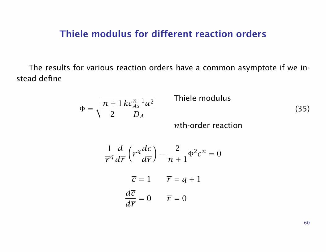
Thiele modulus for different reaction orders
The results for various reaction orders have a common asymptote if we in-stead define
Φ =√√√n+ 1
2kcn−1As a2
DA
Thiele modulus
nth-order reaction
(35)
1rqddr
(rqdcdr
)− 2n+ 1
Φ2cn = 0
c = 1 r = q + 1
dcdr= 0 r = 0
60
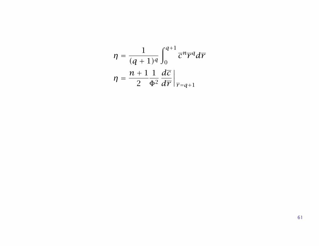
η = 1(q + 1)q
∫ q+1
0cnrqdr
η = n+ 12
1Φ2
dcdr
∣∣∣∣r=q+1
61
Reaction order greater than one
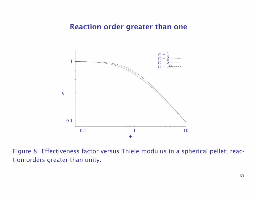
Figure 8 shows the effect of reaction order for n ≥ 1 in a spherical pellet.
As the reaction order increases, the effectiveness factor decreases.
Notice that the definition of Thiele modulus in Equation 35 has achieved thedesired goal of giving all reaction orders a common asymptote at high values ofΦ.
62
Reaction order greater than one
0.1
1
0.1 1 10
η
Φ
n = 1n = 2n = 5n = 10
Figure 8: Effectiveness factor versus Thiele modulus in a spherical pellet; reac-tion orders greater than unity.
63
Reaction order less than one
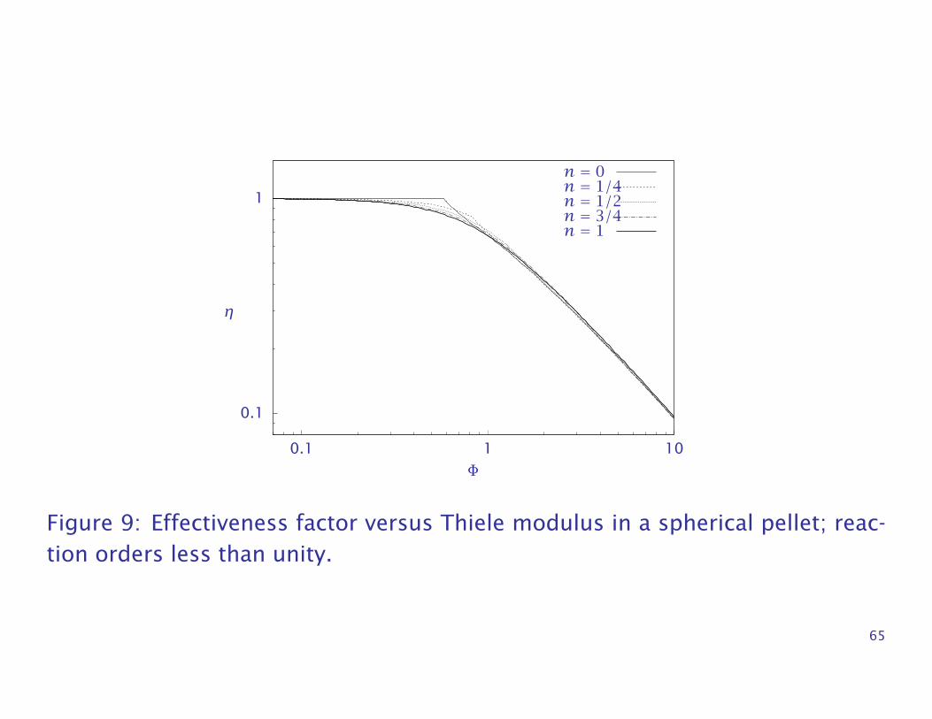
Figure 9 shows the effectiveness factor versus Thiele modulus for reactionorders less than unity.
Notice the discontinuity in slope of the effectiveness factor versus Thielemodulus that occurs when the order is less than unity.
64
0.1
1
0.1 1 10
η
Φ
n = 0n = 1/4n = 1/2n = 3/4n = 1
Figure 9: Effectiveness factor versus Thiele modulus in a spherical pellet; reac-tion orders less than unity.
65
Reaction order less than one
Recall from the discussion in Chapter 4 that if the reaction order is less thanunity in a batch reactor, the concentration of A reaches zero in finite time.
In the reaction-diffusion problem in the pellet, the same kinetic effect causesthe discontinuity in η versus Φ.
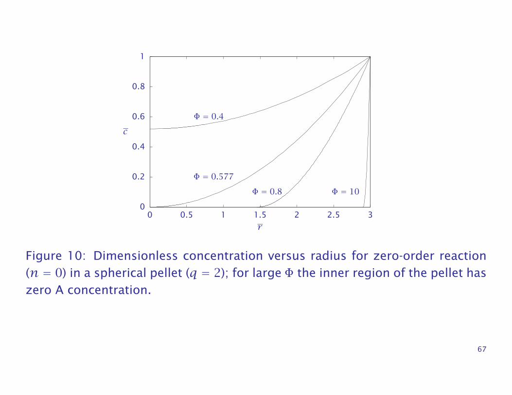
For large values of Thiele modulus, the diffusion is slow compared to reac-tion, and the A concentration reaches zero at some nonzero radius inside thepellet.
For orders less than unity, an inner region of the pellet has identically zeroA concentration.
Figure 10 shows the reactant concentration versus radius for the zero-orderreaction case in a sphere at various values of Thiele modulus.
66
0
0.2
0.4
0.6
0.8
1
0 0.5 1 1.5 2 2.5 3
c
Φ = 0.4
Φ = 0.577
Φ = 0.8 Φ = 10
r
Figure 10: Dimensionless concentration versus radius for zero-order reaction(n = 0) in a spherical pellet (q = 2); for large Φ the inner region of the pellet haszero A concentration.
67
Use the right Φ and ignore reaction order!
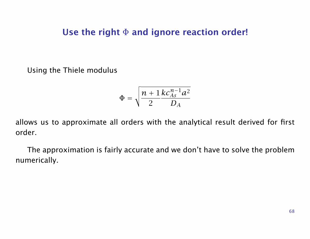
Using the Thiele modulus
Φ =√√√n+ 1
2kcn−1As a2
DA
allows us to approximate all orders with the analytical result derived for firstorder.
The approximation is fairly accurate and we don’t have to solve the problemnumerically.
68
Hougen-Watson Kinetics
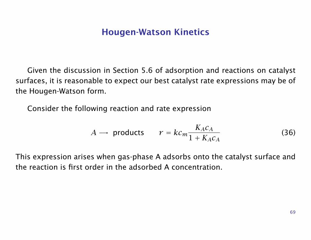
Given the discussion in Section 5.6 of adsorption and reactions on catalystsurfaces, it is reasonable to expect our best catalyst rate expressions may be ofthe Hougen-Watson form.
Consider the following reaction and rate expression
A -→ products r = kcmKAcA
1+KAcA(36)
This expression arises when gas-phase A adsorbs onto the catalyst surface andthe reaction is first order in the adsorbed A concentration.
69
If we consider the slab catalyst geometry, the mass balance is
DAd2cAdr 2
− kcmKAcA
1+KAcA= 0
and the boundary conditions are
cA = cAs r = LdcAdr
= 0 r = 0
We would like to study the effectiveness factor for these kinetics.
70
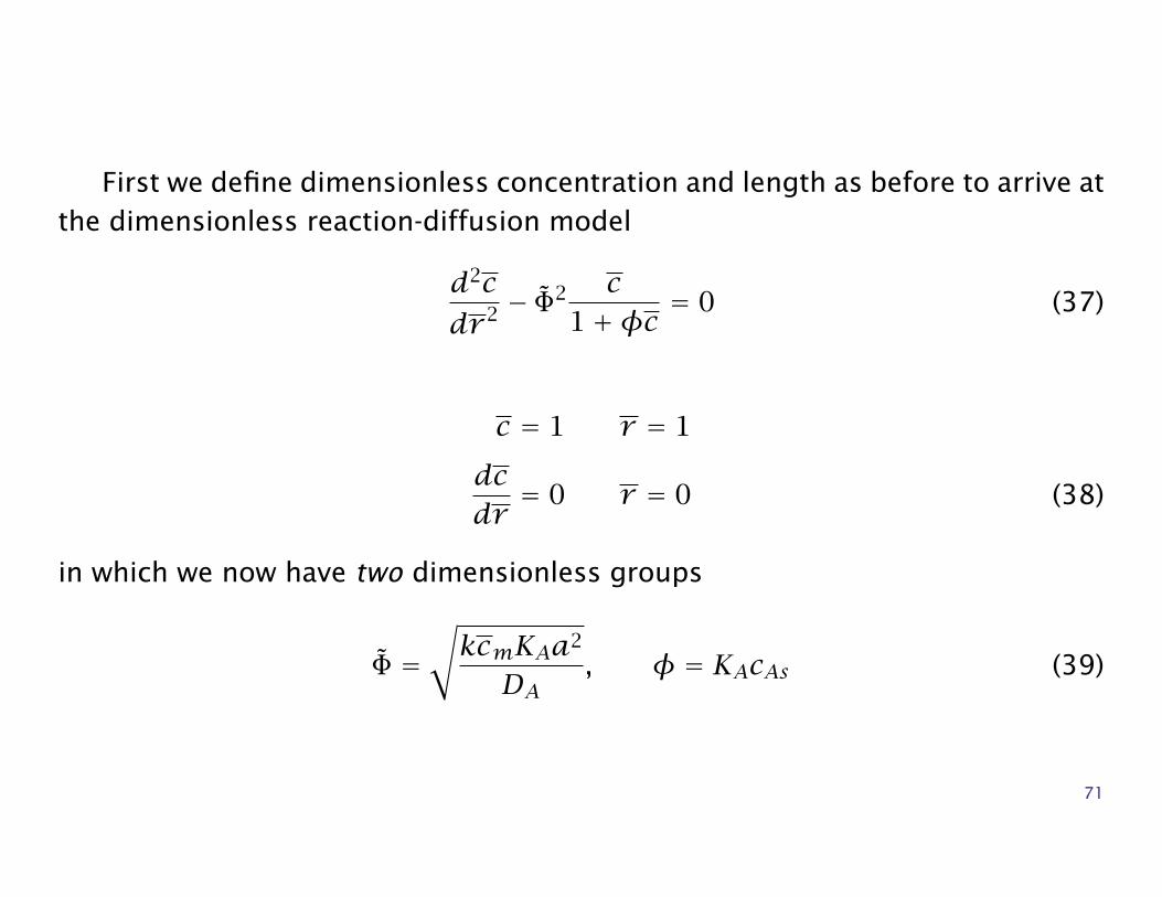
First we define dimensionless concentration and length as before to arrive atthe dimensionless reaction-diffusion model
d2cdr 2 − Φ
2 c1+φc = 0 (37)
c = 1 r = 1
dcdr= 0 r = 0 (38)
in which we now have two dimensionless groups
Φ =√kcmKAa2
DA, φ = KAcAs (39)
71
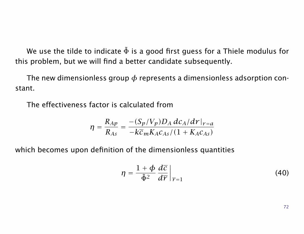
We use the tilde to indicate Φ is a good first guess for a Thiele modulus forthis problem, but we will find a better candidate subsequently.
The new dimensionless groupφ represents a dimensionless adsorption con-stant.
The effectiveness factor is calculated from
η = RApRAs
= −(Sp/Vp)DA dcA/dr |r=a−kcmKAcAs/(1+KAcAs)
which becomes upon definition of the dimensionless quantities
η = 1+φΦ2
dcdr
∣∣∣∣r=1
(40)
72
Rescaling the Thiele modulus
Now we wish to define a Thiele modulus so that η has a common asymptoteat large Φ for all values of φ.
This goal was accomplished for the nth-order reaction as shown in Figures 8and 9 by including the factor (n+1)/2 in the definition of Φ given in Equation 35.
The text shows how to do this analysis, which was developed independentlyby four chemical engineers.
73
What did ChE professors work on in the 1960s?
This idea appears to have been discovered independently by three chemicalengineers in 1965.
To quote from Aris [2, p. 113]
This is the essential idea in three papers published independently in March,May and June of 1965; see Bischoff [4], Aris [1] and Petersen [10]. A morelimited form was given as early as 1958 by Stewart in Bird, Stewart andLightfoot [3, p. 338].
74
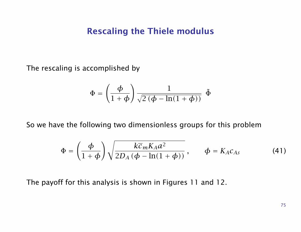
Rescaling the Thiele modulus
The rescaling is accomplished by
Φ =(φ
1+φ
)1√
2 (φ− ln(1+φ)) Φ
So we have the following two dimensionless groups for this problem
Φ =(φ
1+φ
)√kcmKAa2
2DA (φ− ln(1+φ)) , φ = KAcAs (41)
The payoff for this analysis is shown in Figures 11 and 12.
75
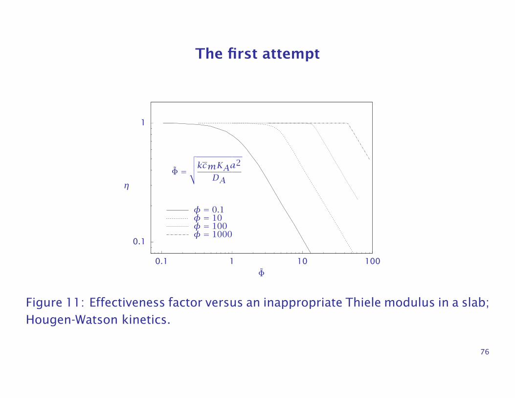
The first attempt
0.1
1
0.1 1 10 100
ηΦ =
√√√√kcmKAa2
DA
Φ
φ = 0.1φ = 10φ = 100φ = 1000
Figure 11: Effectiveness factor versus an inappropriate Thiele modulus in a slab;Hougen-Watson kinetics.
76
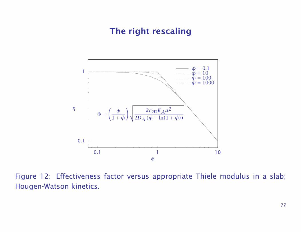
The right rescaling
0.1
1
0.1 1 10
ηΦ =
(φ
1+φ
)√√√√ kcmKAa2
2DA (φ− ln(1+φ))
Φ
φ = 0.1φ = 10φ = 100φ = 1000
Figure 12: Effectiveness factor versus appropriate Thiele modulus in a slab;Hougen-Watson kinetics.
77
Use the right Φ and ignore the reaction form!
If we use our first guess for the Thiele modulus, Equation 39, we obtainFigure 11 in which the various values of φ have different asymptotes.
Using the Thiele modulus defined in Equation 41, we obtain the results inFigure 12. Figure 12 displays things more clearly.
Again we see that as long as we choose an appropriate Thiele modulus, wecan approximate the effectiveness factor for all values of φ with the first-orderreaction.
The largest approximation error occurs near Φ = 1, and if Φ > 2 or Φ < 0.2,the approximation error is negligible.
78
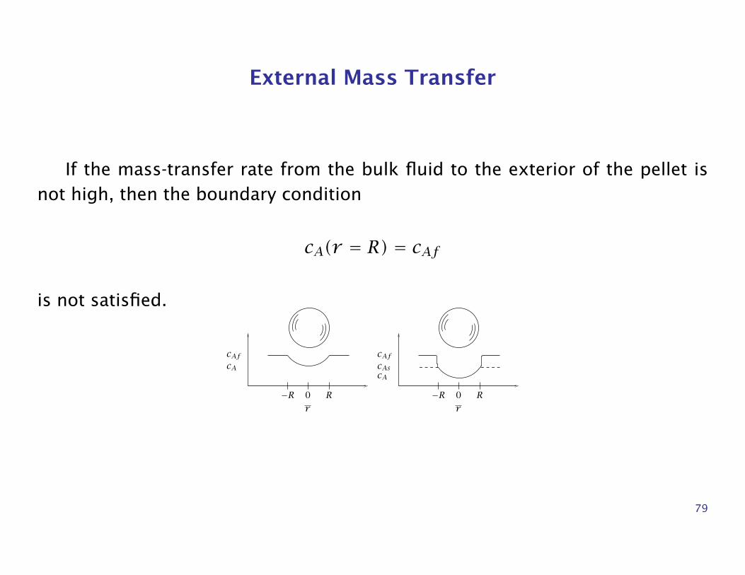
External Mass Transfer
If the mass-transfer rate from the bulk fluid to the exterior of the pellet isnot high, then the boundary condition
cA(r = R) = cAf
is not satisfied.
0−R Rr
0−R Rr
cAfcAs
cAfcA
cA
79
Mass transfer boundary condition
To obtain a simple model of the external mass transfer, we replace theboundary condition above with a flux boundary condition
DAdcAdr
= km(cAf − cA
), r = R (42)
in which km is the external mass-transfer coefficient.
If we multiply Equation 42 by a/cAfDA, we obtain the dimensionless bound-ary condition
dcdr= B (1− c) , r = 3 (43)
in which
B = kmaDA
(44)
is the Biot number or dimensionless mass-transfer coefficient.
80
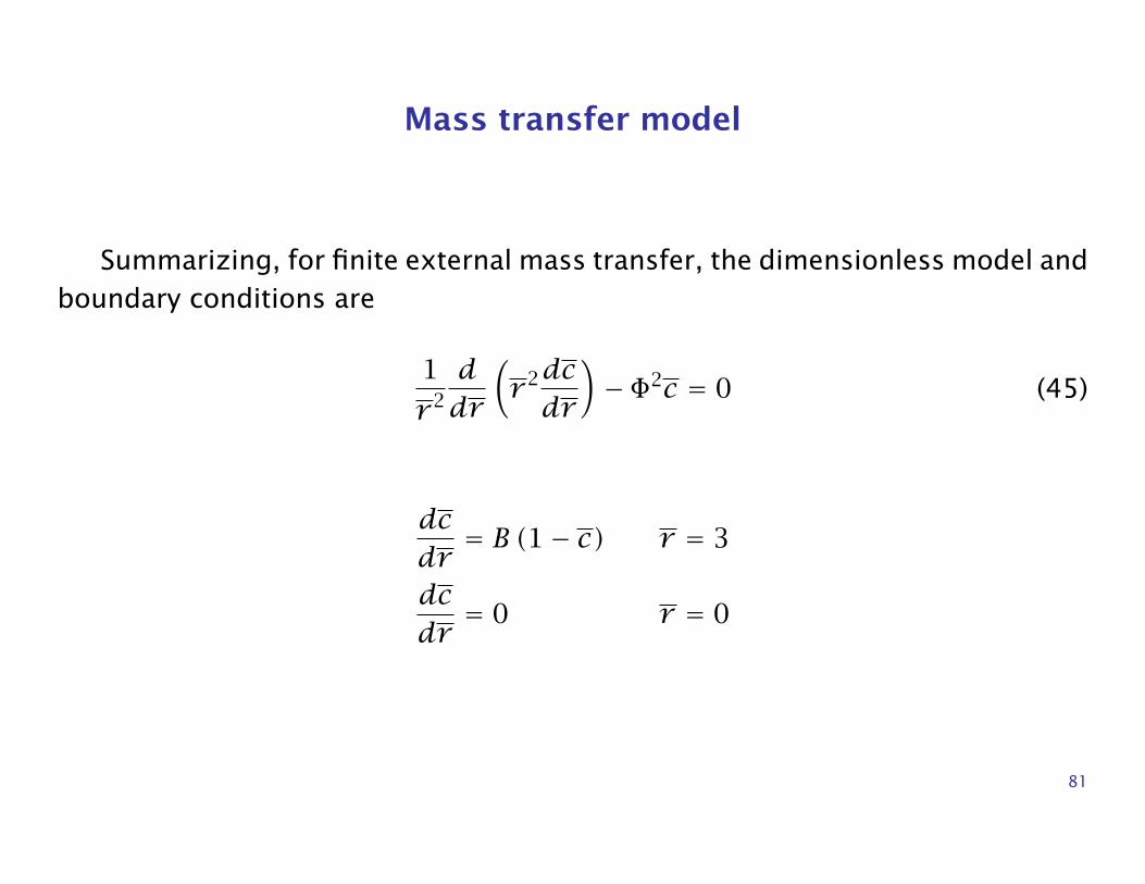
Mass transfer model
Summarizing, for finite external mass transfer, the dimensionless model andboundary conditions are
1
r 2
ddr
(r 2dcdr
)− Φ2c = 0 (45)
dcdr= B (1− c) r = 3
dcdr= 0 r = 0
81
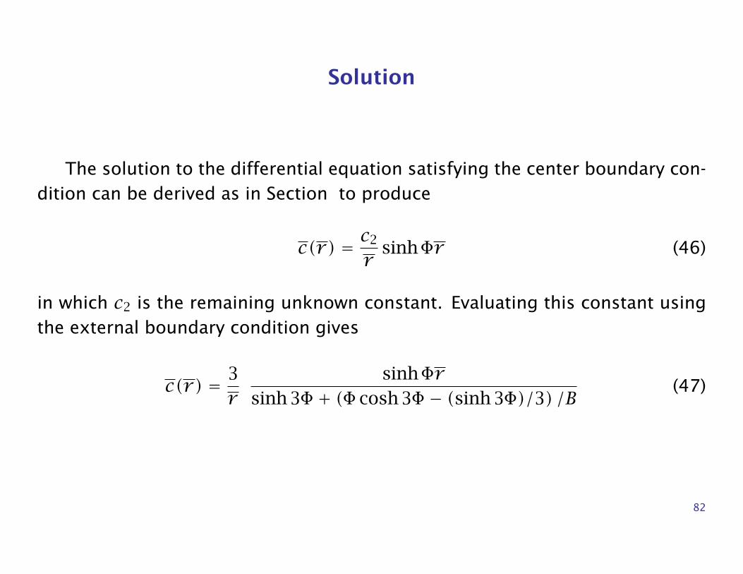
Solution
The solution to the differential equation satisfying the center boundary con-dition can be derived as in Section to produce
c(r) = c2
rsinhΦr (46)
in which c2 is the remaining unknown constant. Evaluating this constant usingthe external boundary condition gives
c(r) = 3r
sinhΦrsinh 3Φ + (Φ cosh 3Φ − (sinh 3Φ)/3) /B
(47)
82
0
0.1
0.2
0.3
0.4
0.5
0.6
0.7
0.8
0.9
1
0 0.5 1 1.5 2 2.5 3
c
B = ∞
2.0
0.5
0.1
r
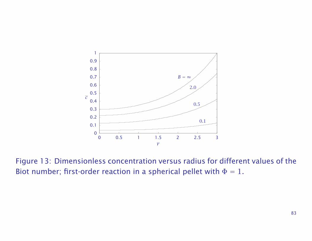
Figure 13: Dimensionless concentration versus radius for different values of theBiot number; first-order reaction in a spherical pellet with Φ = 1.
83
Effectiveness Factor
The effectiveness factor can again be derived by integrating the local reactionrate or computing the surface flux, and the result is
η = 1Φ
[1/ tanh 3Φ − 1/(3Φ)
1+ Φ (1/ tanh 3Φ − 1/(3Φ)) /B
](48)
in which
η = RApRAb
Notice we are comparing the pellet’s reaction rate to the rate that would beachieved if the pellet reacted at the bulk fluid concentration rather than thepellet exterior concentration as before.
84
10−5
10−4
10−3
10−2
10−1
1
0.01 0.1 1 10 100
B=∞
2.0
0.5
0.1
η
Φ
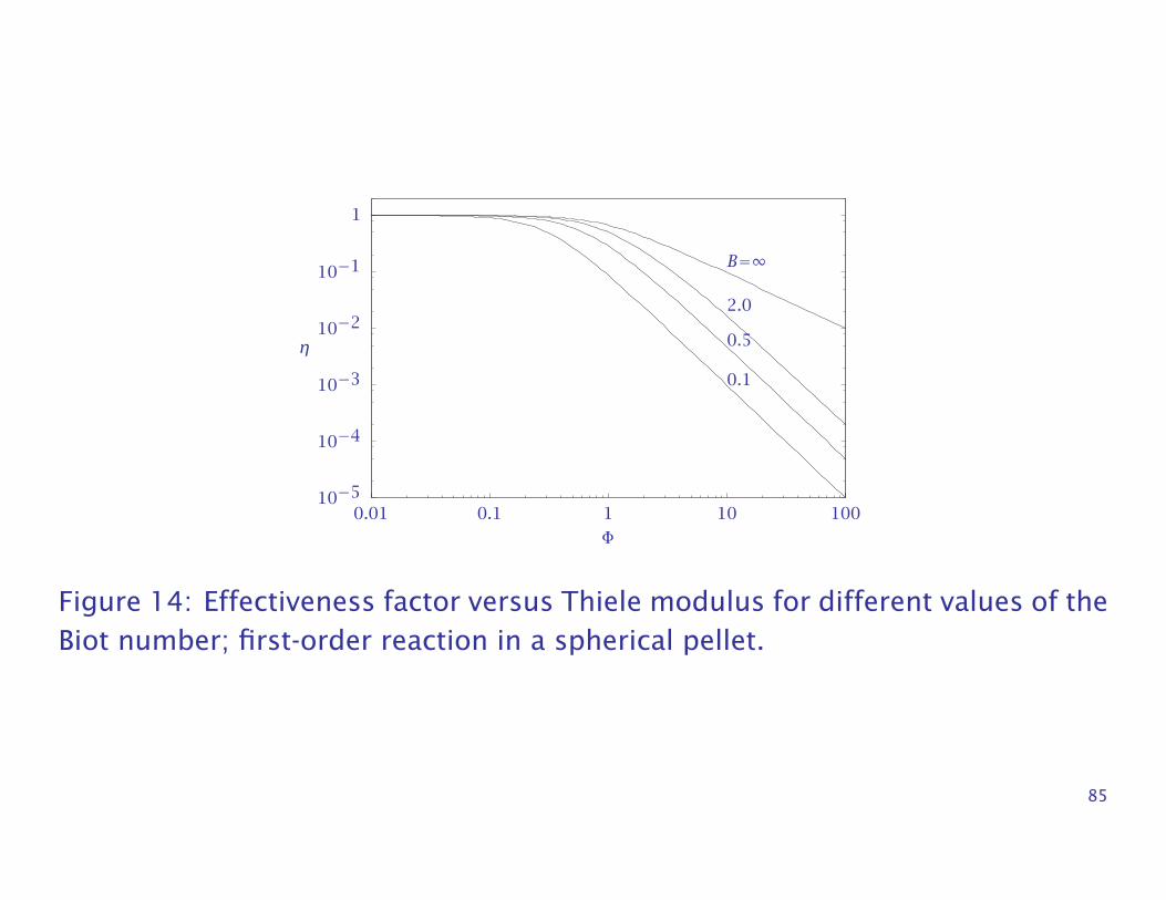
Figure 14: Effectiveness factor versus Thiele modulus for different values of theBiot number; first-order reaction in a spherical pellet.
85
Figure 14 shows the effect of the Biot number on the effectiveness factor ortotal pellet reaction rate.
Notice that the slope of the log-log plot of η versus Φ has a slope of nega-tive two rather than negative one as in the case without external mass-transferlimitations (B = ∞).
Figure 15 shows this effect in more detail.
86
10−6
10−5
10−4
10−3
10−2
10−1
1
10−2 10−1 1 101 102 103 104
B1 = 0.01
B2 = 100
√B1
√B2
η
Φ
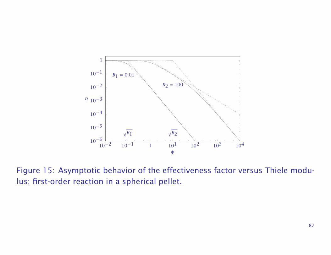
Figure 15: Asymptotic behavior of the effectiveness factor versus Thiele modu-lus; first-order reaction in a spherical pellet.
87
Making a sketch of η versus Φ
If B is small, the log-log plot corners with a slope of negative two at Φ =√B.
If B is large, the log-log plot first corners with a slope of negative one atΦ = 1, then it corners again and decreases the slope to negative two at Φ =
√B.
Both mechanisms of diffusional resistance, the diffusion within the pellet andthe mass transfer from the fluid to the pellet, show their effect on pellet reactionrate by changing the slope of the effectiveness factor by negative one.
Given the value of the Biot number, one can easily sketch the straight lineasymptotes shown in Figure 15. Then, given the value of the Thiele modulus,one can determine the approximate concentration profile, and whether internaldiffusion or external mass transfer or both limit the pellet reaction rate.
88
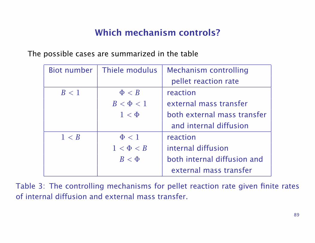
Which mechanism controls?
The possible cases are summarized in the table
Biot number Thiele modulus Mechanism controlling
pellet reaction rate
B < 1 Φ < B reaction
B < Φ < 1 external mass transfer
1 < Φ both external mass transfer
and internal diffusion
1 < B Φ < 1 reaction
1 < Φ < B internal diffusion
B < Φ both internal diffusion and
external mass transfer
Table 3: The controlling mechanisms for pellet reaction rate given finite ratesof internal diffusion and external mass transfer.
89
Observed versus Intrinsic Kinetic Parameters
• We often need to determine a reaction order and rate constant for some cat-alytic reaction of interest.
• Assume the following nth-order reaction takes place in a catalyst particle
A -→ B, r1 = kcnA
• We call the values of k and n the intrinsic rate constant and reaction order todistinguish them from what we may estimate from data.
• The typical experiment is to change the value of cA in the bulk fluid, measurethe rate r1 as a function of cA, and then find the values of the parameters kand n that best fit the measurements.
90
Observed versus Intrinsic Kinetic Parameters
Here we show only that one should exercise caution with this estimation if weare measuring the rates with a solid catalyst. The effects of reaction, diffusionand external mass transfer may all manifest themselves in the measured rate.
We express the reaction rate as
r1 = ηkcnAb (49)
We also know that at steady state, the rate is equal to the flux of A into thecatalyst particle
r1 = kmA(cAb − cAs) =DAadcAdr
∣∣∣∣r=R
(50)
We now study what happens to our experiment under different rate-limitingsteps.
91
Reaction limited
First assume that both the external mass transfer and internal pellet diffusionare fast compared to the reaction. Then η = 1, and we would estimate theintrinsic parameters correctly in Equation 49
kob = k
nob = n
Everything goes according to plan when we are reaction limited.
92
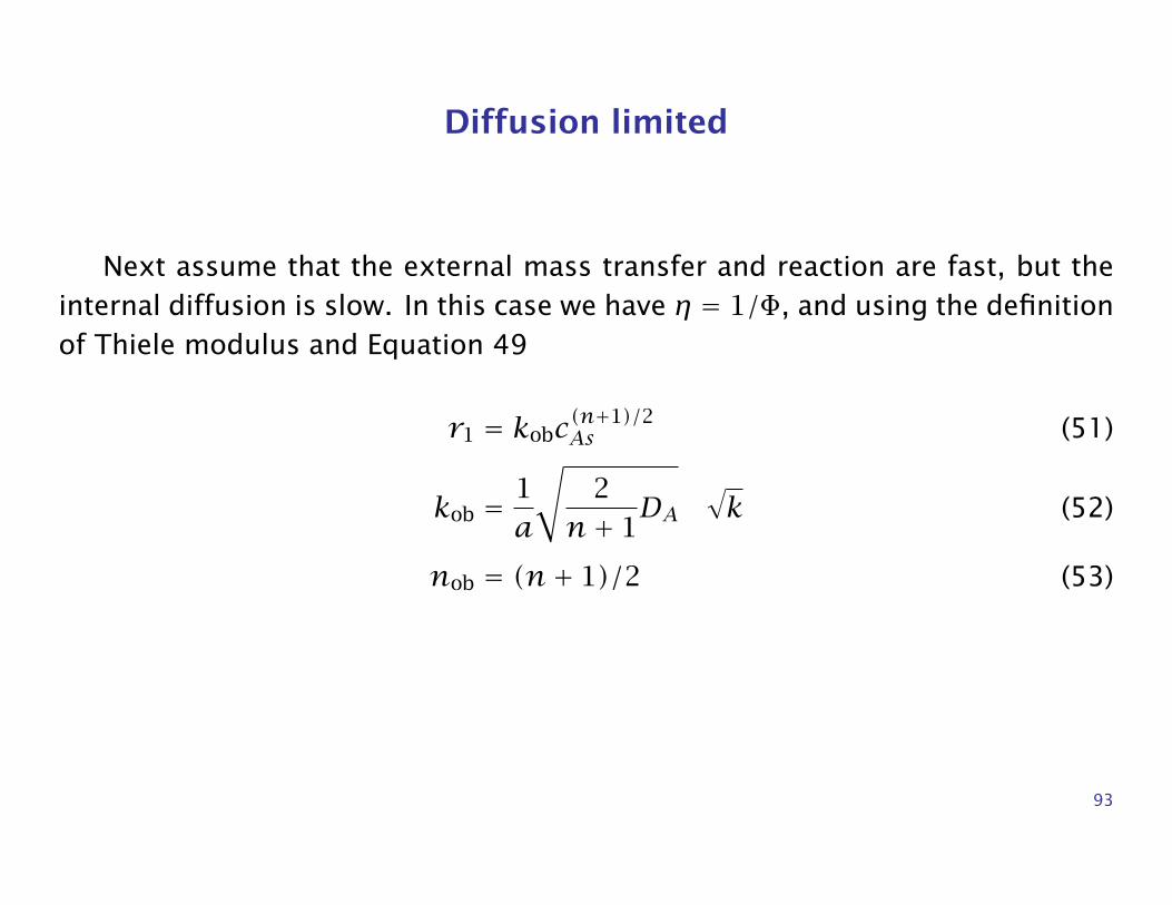
Diffusion limited
Next assume that the external mass transfer and reaction are fast, but theinternal diffusion is slow. In this case we have η = 1/Φ, and using the definitionof Thiele modulus and Equation 49
r1 = kobc(n+1)/2As (51)
kob =1a
√2
n+ 1DA
√k (52)
nob = (n+ 1)/2 (53)
93
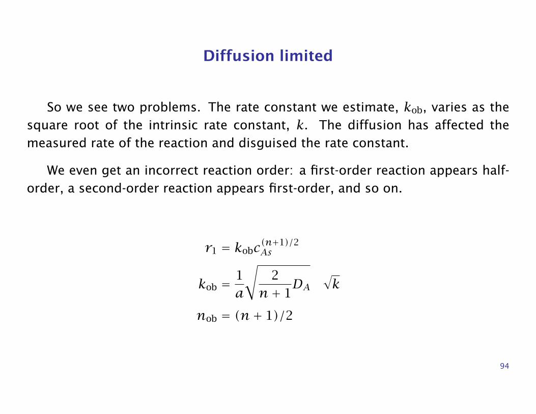
Diffusion limited
So we see two problems. The rate constant we estimate, kob, varies as thesquare root of the intrinsic rate constant, k. The diffusion has affected themeasured rate of the reaction and disguised the rate constant.
We even get an incorrect reaction order: a first-order reaction appears half-order, a second-order reaction appears first-order, and so on.
r1 = kobc(n+1)/2As
kob =1a
√2
n+ 1DA
√k
nob = (n+ 1)/2
94
Diffusion limited
Also consider what happens if we vary the temperature and try to determinethe reaction’s activation energy.
Let the temperature dependence of the diffusivity, DA, be represented alsoin Arrhenius form, with Ediff the activation energy of the diffusion coefficient.
Let Erxn be the intrinsic activation energy of the reaction. The observed acti-vation energy from Equation 52 is
Eob =Ediff + Erxn
2
so both activation energies show up in our estimated activation energy.
Normally the temperature dependence of the diffusivity is much smaller than
95
the temperature dependence of the reaction, Ediff Erxn, so we would estimatean activation energy that is one-half the intrinsic value.
96
Mass transfer limited
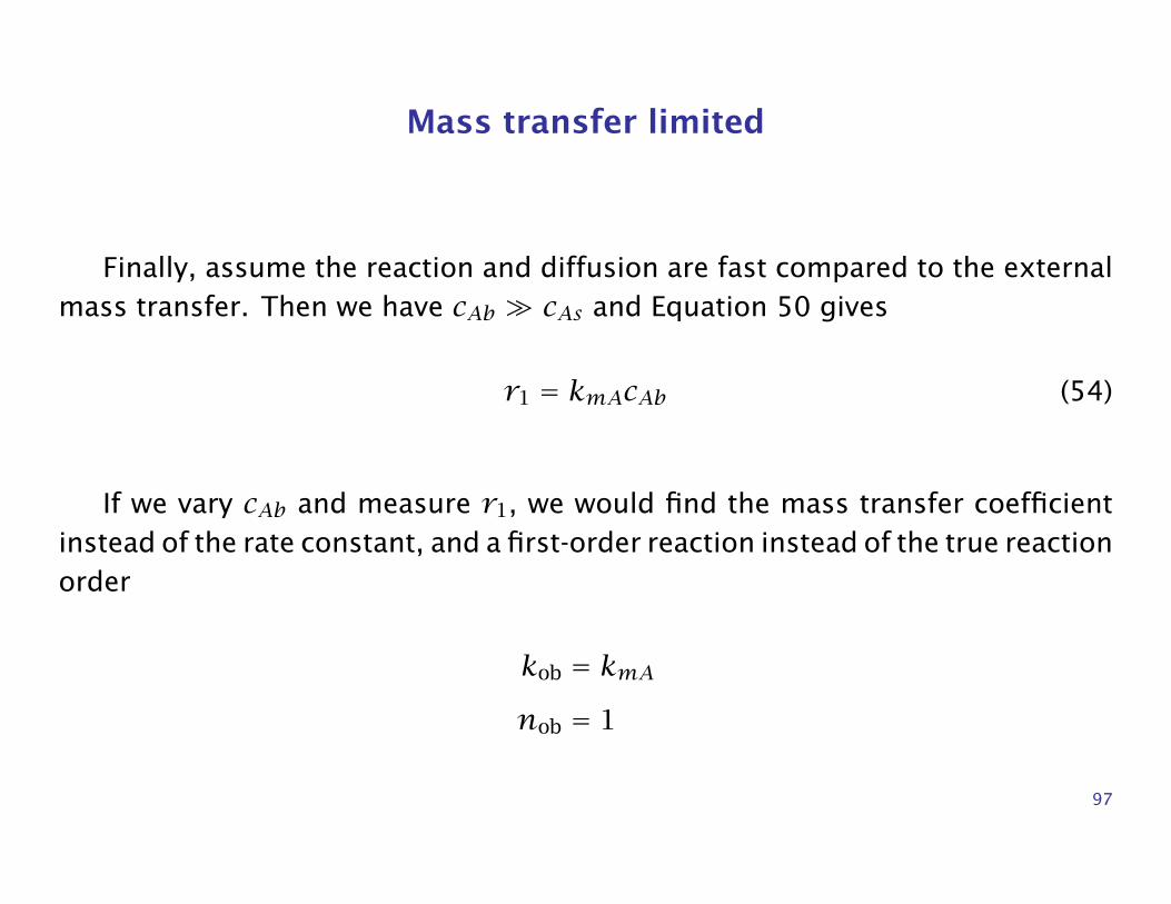
Finally, assume the reaction and diffusion are fast compared to the externalmass transfer. Then we have cAb cAs and Equation 50 gives
r1 = kmAcAb (54)
If we vary cAb and measure r1, we would find the mass transfer coefficientinstead of the rate constant, and a first-order reaction instead of the true reactionorder
kob = kmAnob = 1
97
Normally, mass-transfer coefficients also have fairly small temperature de-pendence compared to reaction rates, so the observed activation energy wouldbe almost zero, independent of the true reaction’s activation energy.
98
Moral to the story
Mass transfer and diffusion resistances disguise the reaction kinetics.
We can solve this problem in two ways. First, we can arrange the experimentso that mass transfer and diffusion are fast and do not affect the estimates ofthe kinetic parameters. How?
If this approach is impractical or too expensive, we can alternatively modelthe effects of the mass transfer and diffusion, and estimate the parameters DAand kmA simultaneously with k and n. We develop techniques in Chapter 9 tohandle this more complex estimation problem.
99
Nonisothermal Particle Considerations
• We now consider situations in which the catalyst particle is not isothermal.
• Given an exothermic reaction, for example, if the particle’s thermal conductiv-ity is not large compared to the rate of heat release due to chemical reaction,the temperature rises inside the particle.
• We wish to explore the effects of this temperature rise on the catalyst perfor-mance.
100
Single, first-order reaction
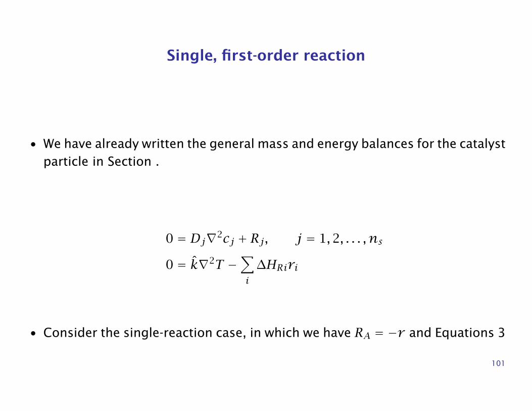
• We have already written the general mass and energy balances for the catalystparticle in Section .
0 = Dj∇2cj + Rj, j = 1,2, . . . , ns
0 = k∇2T −∑i∆HRiri
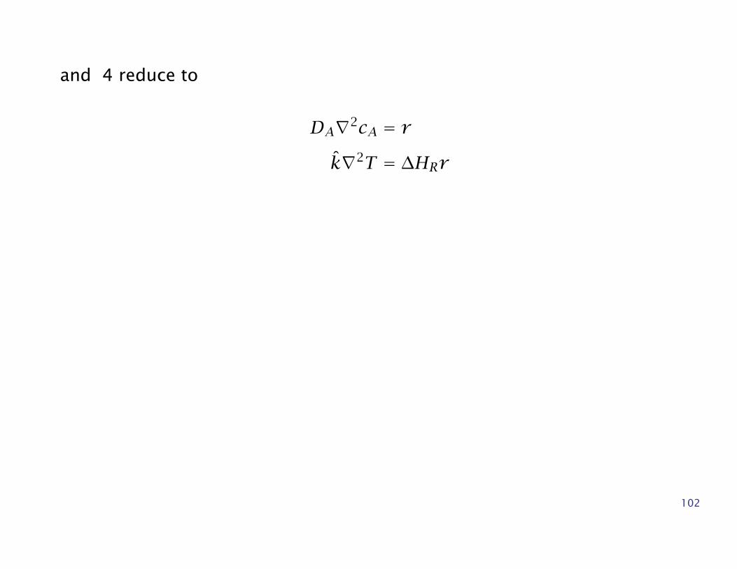
• Consider the single-reaction case, in which we have RA = −r and Equations 3
101
and 4 reduce to
DA∇2cA = r
k∇2T = ∆HRr
102
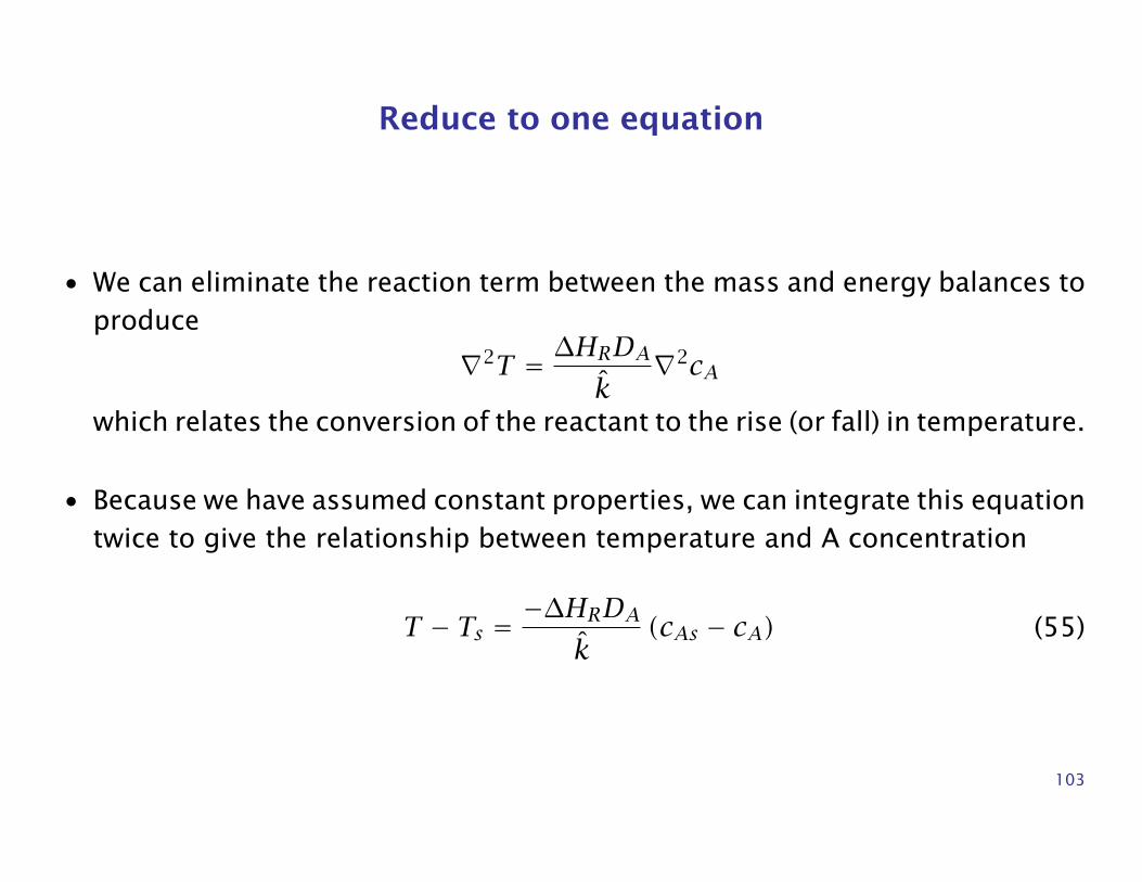
Reduce to one equation
• We can eliminate the reaction term between the mass and energy balances toproduce
∇2T = ∆HRDAk
∇2cA
which relates the conversion of the reactant to the rise (or fall) in temperature.
• Because we have assumed constant properties, we can integrate this equationtwice to give the relationship between temperature and A concentration
T − Ts =−∆HRDA
k(cAs − cA) (55)
103
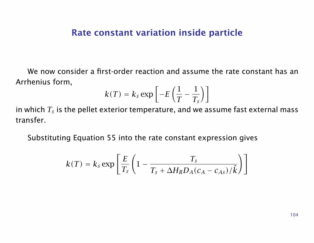
Rate constant variation inside particle
We now consider a first-order reaction and assume the rate constant has anArrhenius form,
k(T) = ks exp[−E
(1T− 1Ts
)]in which Ts is the pellet exterior temperature, and we assume fast external masstransfer.
Substituting Equation 55 into the rate constant expression gives
k(T) = ks exp
[ETs
(1− Ts
Ts +∆HRDA(cA − cAs)/k
)]
104
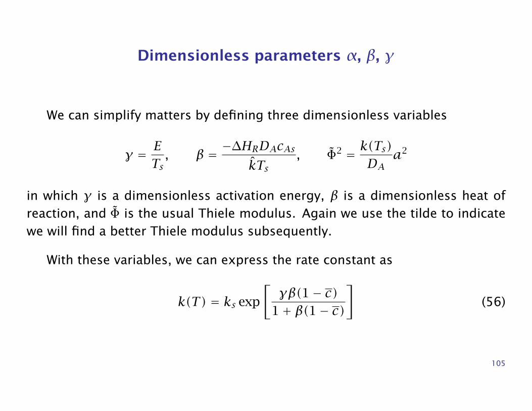
Dimensionless parameters α, β, γ
We can simplify matters by defining three dimensionless variables
γ = ETs, β = −∆HRDAcAs
kTs, Φ2 = k(Ts)
DAa2
in which γ is a dimensionless activation energy, β is a dimensionless heat ofreaction, and Φ is the usual Thiele modulus. Again we use the tilde to indicatewe will find a better Thiele modulus subsequently.
With these variables, we can express the rate constant as
k(T) = ks exp
[γβ(1− c)
1+ β(1− c)
](56)
105
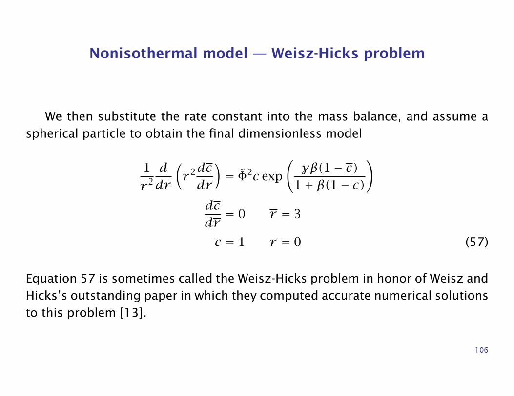
Nonisothermal model — Weisz-Hicks problem
We then substitute the rate constant into the mass balance, and assume aspherical particle to obtain the final dimensionless model
1
r 2
ddr
(r 2dcdr
)= Φ2c exp
(γβ(1− c)
1+ β(1− c)
)dcdr= 0 r = 3
c = 1 r = 0 (57)
Equation 57 is sometimes called the Weisz-Hicks problem in honor of Weisz andHicks’s outstanding paper in which they computed accurate numerical solutionsto this problem [13].
106
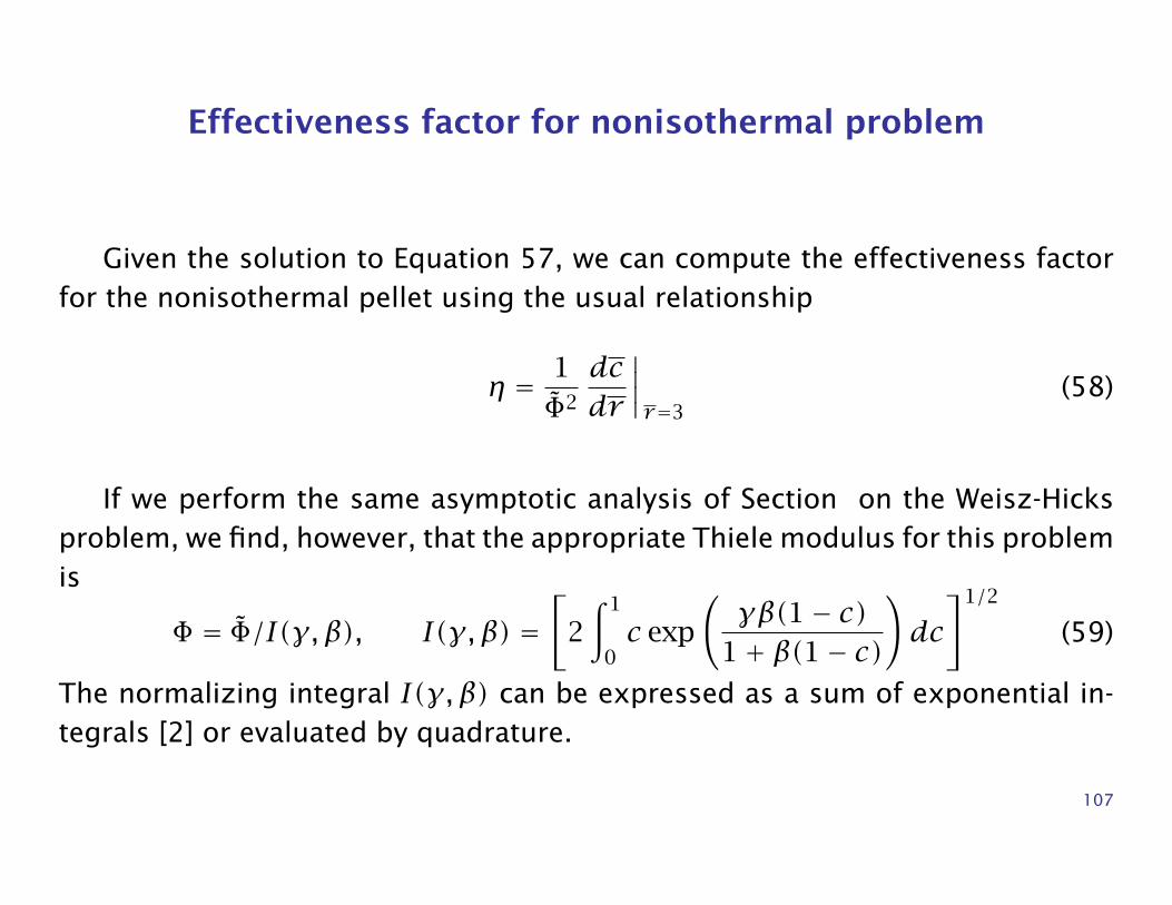
Effectiveness factor for nonisothermal problem
Given the solution to Equation 57, we can compute the effectiveness factorfor the nonisothermal pellet using the usual relationship
η = 1Φ2
dcdr
∣∣∣∣r=3
(58)
If we perform the same asymptotic analysis of Section on the Weisz-Hicksproblem, we find, however, that the appropriate Thiele modulus for this problemis
Φ = Φ/I(γ, β), I(γ, β) =[
2∫ 1
0c exp
(γβ(1− c)
1+ β(1− c)
)dc]1/2
(59)
The normalizing integral I(γ, β) can be expressed as a sum of exponential in-tegrals [2] or evaluated by quadrature.
107
10−1
1
101
102
103
10−4 10−3 10−2 10−1 1 101
β=0.60.4
0.3
0.20.1
β=0,−0.8
γ = 30
•
•
•
A
B
C
η
Φ
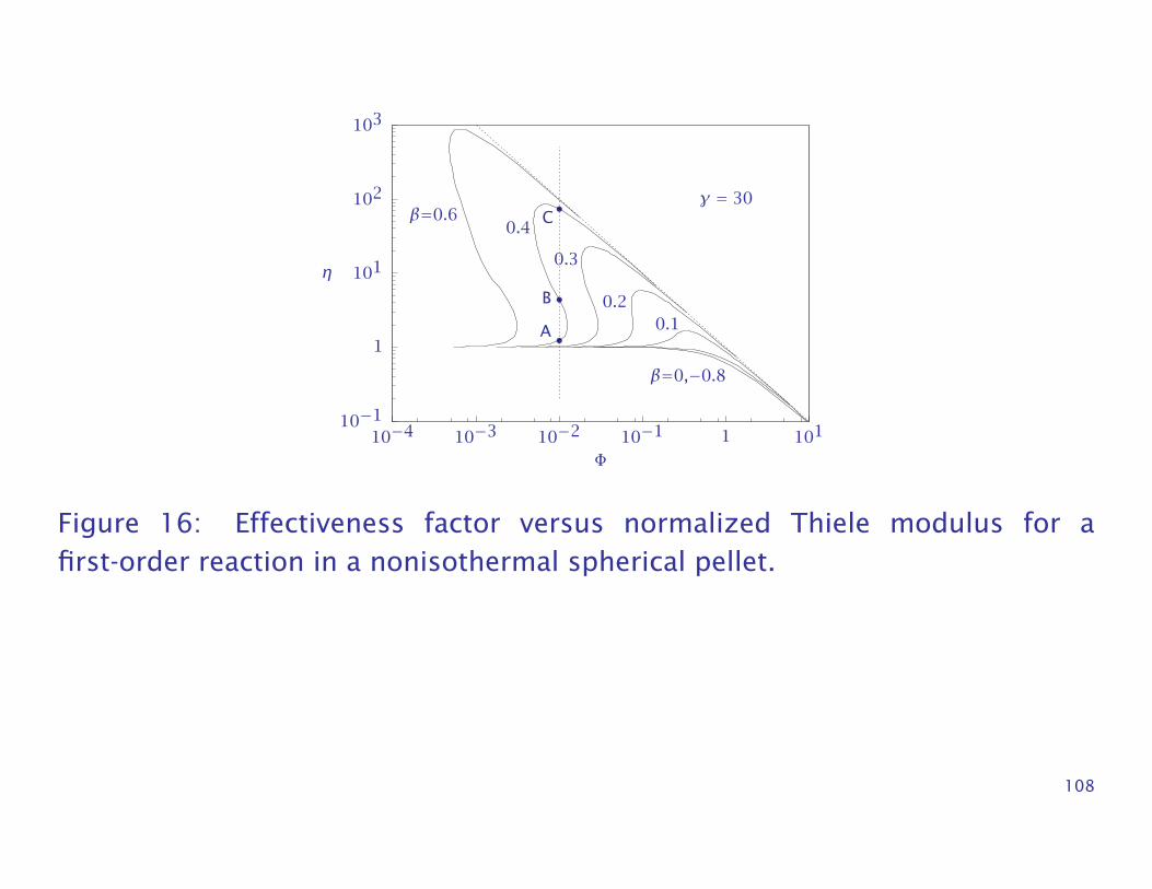
Figure 16: Effectiveness factor versus normalized Thiele modulus for afirst-order reaction in a nonisothermal spherical pellet.
108
• Note that Φ is well chosen in Equation 59 because the large Φ asymptotes arethe same for all values of γ and β.
• The first interesting feature of Figure 16 is that the effectiveness factor isgreater than unity for some values of the parameters.
• Notice that feature is more pronounced as we increase the exothermic heatof reaction.
• For the highly exothermic case, the pellet’s interior temperature is signifi-cantly higher than the exterior temperature Ts. The rate constant inside thepellet is therefore much larger than the value at the exterior, ks. This leadsto η greater than unity.
109
• A second striking feature of the nonisothermal pellet is that multiple steadystates are possible.
• Consider the case Φ = 0.01, β = 0.4 and γ = 30 shown in Figure 16.
• The effectiveness factor has three possible values for this case.
• We show in the next two figures the solution to Equation 57 for this case.
110
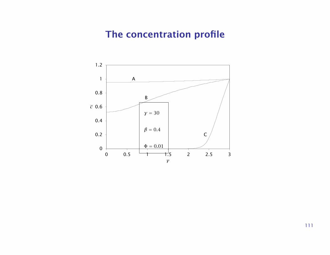
The concentration profile
0
0.2
0.4
0.6
0.8
1
1.2
0 0.5 1 1.5 2 2.5 3
c
C
B
A
γ = 30
β = 0.4
Φ = 0.01
r
111
And the temperature profile
0
0.1
0.2
0.3
0.4
0.5
0 0.5 1 1.5 2 2.5 3
T
A
B
Cγ = 30
β = 0.4
Φ = 0.01
r
112
MSS in nonisothermal pellet
• The three temperature and concentration profiles correspond to an ignitedsteady state (C), an extinguished steady state (A), and an unstable interme-diate steady state (B).
• As we showed in Chapter 6, whether we achieve the ignited or extinguishedsteady state in the pellet depends on how the reactor is started.
• For realistic values of the catalyst thermal conductivity, however, the pel-let can often be considered isothermal and the energy balance can be ne-glected [9].
• Multiple steady-state solutions in the particle may still occur in practice, how-ever, if there is a large external heat transfer resistance.
113
Multiple Reactions
• As the next step up in complexity, we consider the case of multiple reactions.
• Even numerical solution of some of these problems is challenging for tworeasons.
• First, steep concentration profiles often occur for realistic parameter values,and we wish to compute these profiles accurately. It is not unusual for speciesconcentrations to change by 10 orders of magnitude within the pellet forrealistic reaction and diffusion rates.
• Second, we are solving boundary-value problems because the boundary con-ditions are provided at the center and exterior surface of the pellet.
114
• We use the collocation method, which is described in more detail in Ap-pendix A.
115
Multiple reaction example — Catalytic converter
The next example involves five species, two reactions with Hougen-Watsonkinetics, and both diffusion and external mass-transfer limitations.
Consider the oxidation of CO and a representative volatile organic such aspropylene in a automobile catalytic converter containing spherical catalyst pel-lets with particle radius 0.175 cm.
The particle is surrounded by a fluid at 1.0 atm pressure and 550 K containing2% CO, 3% O2 and 0.05% (500 ppm) C3H6. The reactions of interest are
CO+ 12
O2 -→ CO2 (60)
C3H6 +92
O2 -→ 3CO2 + 3H2O (61)
116
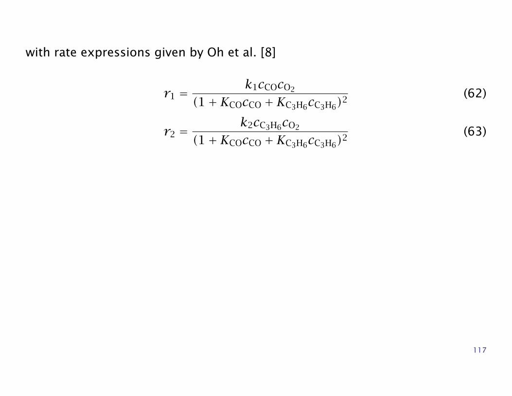
with rate expressions given by Oh et al. [8]
r1 =k1cCOcO2
(1+KCOcCO +KC3H6cC3H6)2(62)
r2 =k2cC3H6cO2
(1+KCOcCO +KC3H6cC3H6)2(63)
117
Catalytic converter
The rate constants and the adsorption constants are assumed to have Arrhe-nius form.
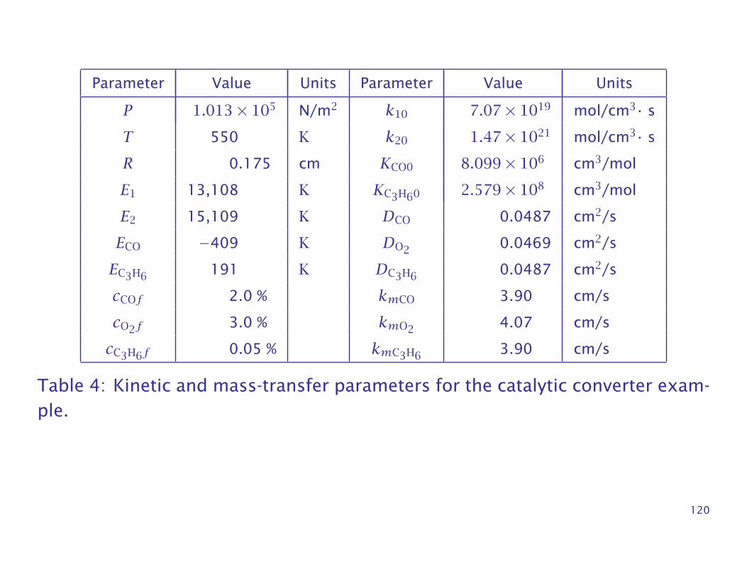
The parameter values are given in Table 4 [8].
The pellet may be assumed to be isothermal.
Calculate the steady-state pellet concentration profiles of all reactants andproducts.
118
Data
119
Parameter Value Units Parameter Value Units
P 1.013× 10⁵ N/m2 k10 7.07× 10¹⁹ mol/cm3· s
T 550 K k20 1.47× 10²¹ mol/cm3· s
R 0.175 cm KCO0 8.099× 106 cm3/mol
E1 13,108 K KC3H60 2.579× 108 cm3/mol
E2 15,109 K DCO 0.0487 cm2/s
ECO −409 K DO2 0.0469 cm2/s
EC3H6 191 K DC3H6 0.0487 cm2/s
cCOf 2.0 % kmCO 3.90 cm/s
cO2f 3.0 % kmO2 4.07 cm/s
cC3H6f 0.05 % kmC3H6 3.90 cm/s
Table 4: Kinetic and mass-transfer parameters for the catalytic converter exam-ple.
120
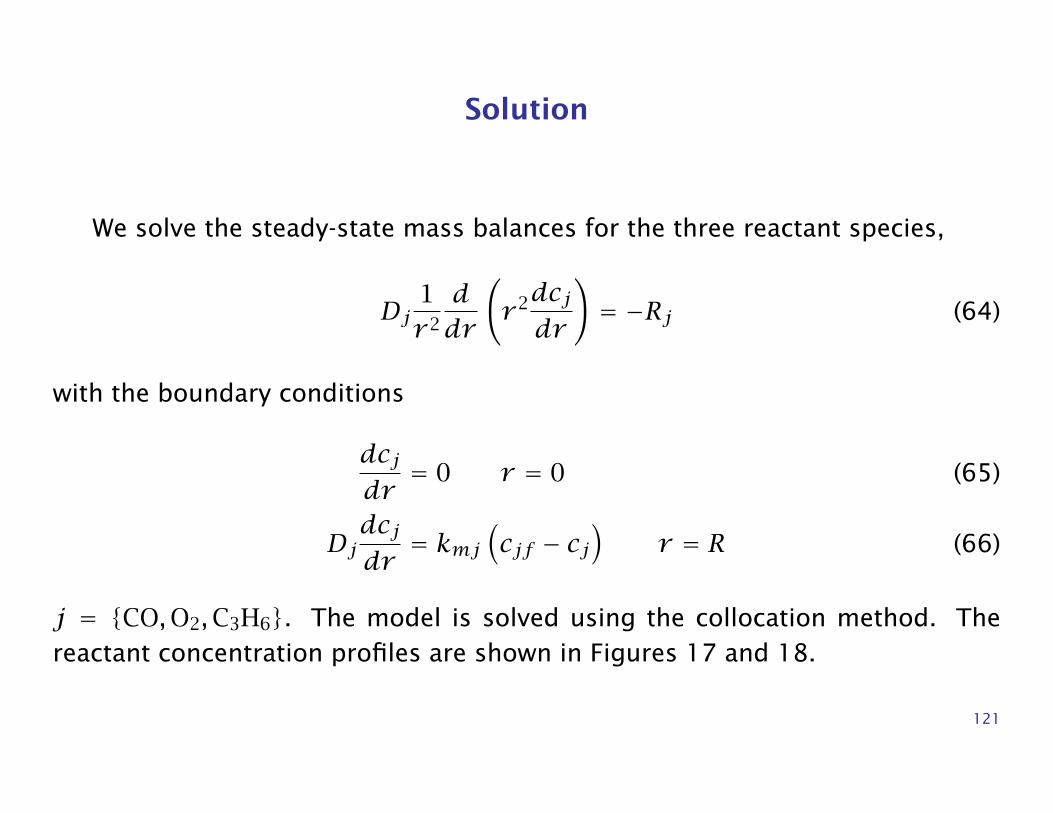
Solution
We solve the steady-state mass balances for the three reactant species,
Dj1r 2
ddr
(r 2dcjdr
)= −Rj (64)
with the boundary conditions
dcjdr= 0 r = 0 (65)
Djdcjdr= kmj
(cjf − cj
)r = R (66)
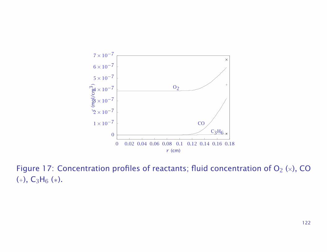
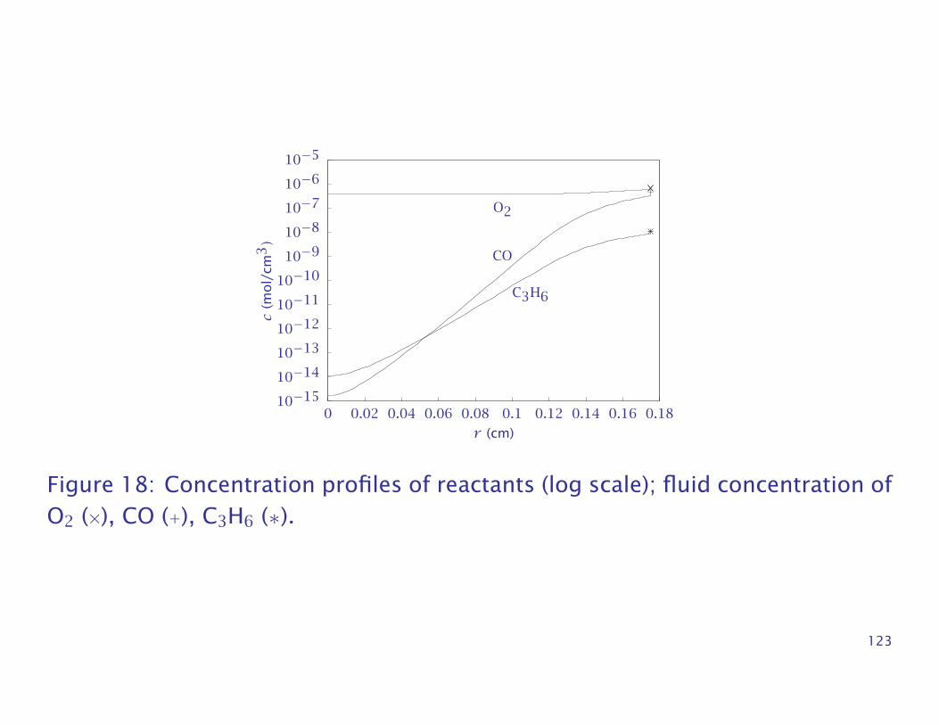
j = CO,O2,C3H6. The model is solved using the collocation method. Thereactant concentration profiles are shown in Figures 17 and 18.
121
0
1× 10⁻⁷
2× 10⁻⁷
3× 10⁻⁷
4× 10⁻⁷
5× 10⁻⁷
6× 10⁻⁷
7× 10⁻⁷
0 0.02 0.04 0.06 0.08 0.1 0.12 0.14 0.16 0.18
O2
CO
C3H6
c(m
ol/
cm3)
r (cm)
Figure 17: Concentration profiles of reactants; fluid concentration of O2 (×), CO(+), C3H6 (∗).
122
10−1510−1410−1310−1210−1110−10
10−910−810−710−610−5
0 0.02 0.04 0.06 0.08 0.1 0.12 0.14 0.16 0.18
O2
CO
C3H6
c(m
ol/
cm3)
r (cm)
Figure 18: Concentration profiles of reactants (log scale); fluid concentration ofO2 (×), CO (+), C3H6 (∗).
123
Results
Notice that O2 is in excess and both CO and C3H6 reach very low values withinthe pellet.
The log scale in Figure 18 shows that the concentrations of these reactantschange by seven orders of magnitude.
Obviously the consumption rate is large compared to the diffusion rate forthese species.
The external mass-transfer effect is noticeable, but not dramatic.
124
Product Concentrations
The product concentrations could simply be calculated by solving their massbalances along with those of the reactants.
Because we have only two reactions, however, the products concentrationsare also computable from the stoichiometry and the mass balances.
The text shows this step in detail.
The results of the calculation are shown in the next figure.
125
0
1× 10⁻⁷
2× 10⁻⁷
3× 10⁻⁷
4× 10⁻⁷
5× 10⁻⁷
0 0.02 0.04 0.06 0.08 0.1 0.12 0.14 0.16 0.18
CO2
H2O
c(m
ol/
cm3)
r (cm)
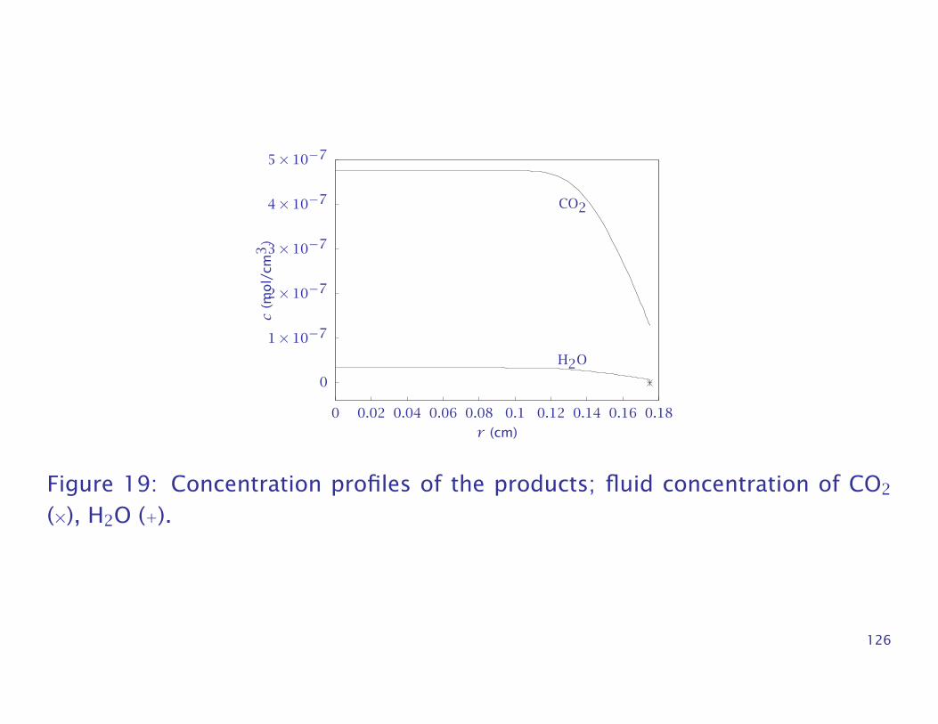
Figure 19: Concentration profiles of the products; fluid concentration of CO2
(×), H2O (+).
126
Product Profiles
Notice from Figure 19 that CO2 is the main product.
Notice also that the products flow out of the pellet, unlike the reactants,which are flowing into the pellet.
127
Fixed-Bed Reactor Design
• Given our detailed understanding of the behavior of a single catalyst particle,we now are prepared to pack a tube with a bed of these particles and solvethe fixed-bed reactor design problem.
• In the fixed-bed reactor, we keep track of two phases. The fluid-phasestreams through the bed and transports the reactants and products throughthe reactor.
• The reaction-diffusion processes take place in the solid-phase catalyst parti-cles.
• The two phases communicate to each other by exchanging mass and energyat the catalyst particle exterior surfaces.
128
• We have constructed a detailed understanding of all these events, and nowwe assemble them together.
129
Coupling the Catalyst and Fluid
We make the following assumptions:
1. Uniform catalyst pellet exterior. Particles are small compared to the lengthof the reactor.
2. Plug flow in the bed, no radial profiles.
3. Neglect axial diffusion in the bed.
4. Steady state.
130
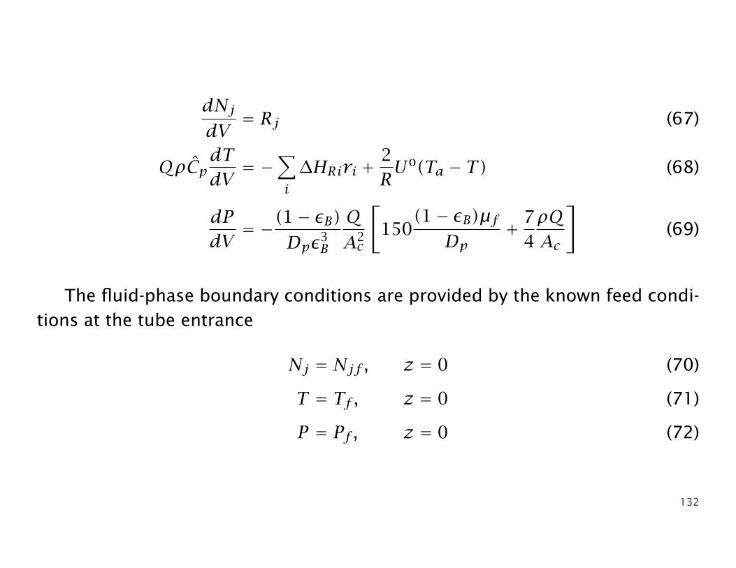
Fluid phase
In the fluid phase, we track the molar flows of all species, the temperatureand the pressure.
We can no longer neglect the pressure drop in the tube because of the catalystbed. We use an empirical correlation to describe the pressure drop in a packedtube, the well-known Ergun equation [6].
131
dNjdV
= Rj (67)
QρCpdTdV= −
∑i∆HRiri +
2RUo(Ta − T) (68)
dPdV= −(1− εB)
Dpε3B
QA2c
[150
(1− εB)µfDp
+ 74ρQAc
](69)
The fluid-phase boundary conditions are provided by the known feed condi-tions at the tube entrance
Nj = Njf , z = 0 (70)
T = Tf , z = 0 (71)
P = Pf , z = 0 (72)
132
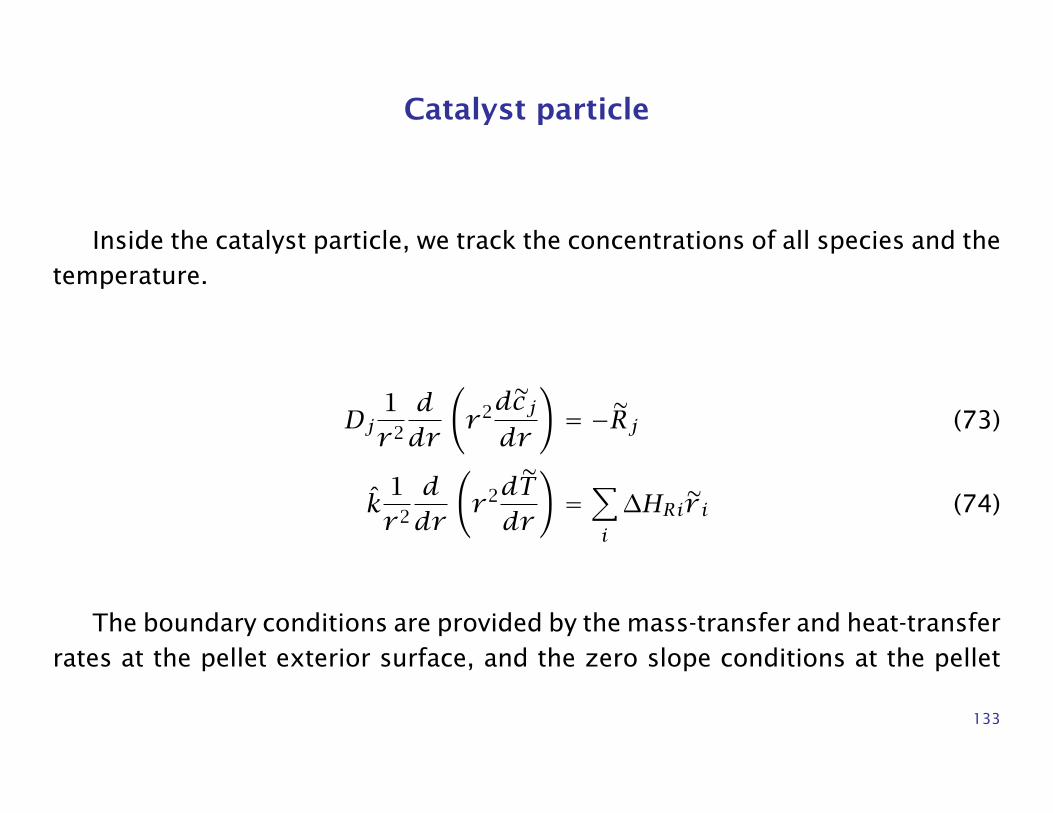
Catalyst particle
Inside the catalyst particle, we track the concentrations of all species and thetemperature.
Dj1r 2
ddr
(r 2dcjdr
)= −Rj (73)
k1r 2
ddr
(r 2dTdr
)=∑i∆HRir i (74)
The boundary conditions are provided by the mass-transfer and heat-transferrates at the pellet exterior surface, and the zero slope conditions at the pellet
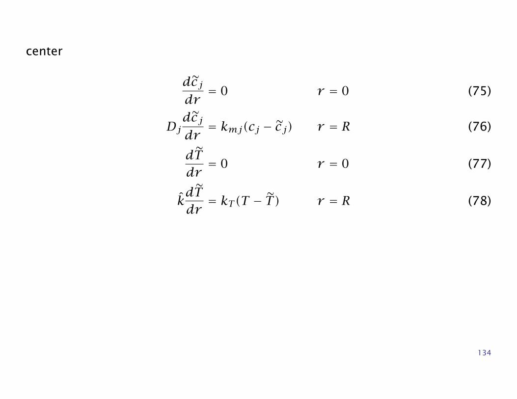
133
center
dcjdr
= 0 r = 0 (75)
Djdcjdr
= kmj(cj − cj) r = R (76)
dTdr= 0 r = 0 (77)
kdTdr= kT(T − T ) r = R (78)
134
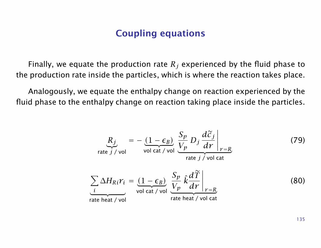
Coupling equations
Finally, we equate the production rate Rj experienced by the fluid phase tothe production rate inside the particles, which is where the reaction takes place.
Analogously, we equate the enthalpy change on reaction experienced by thefluid phase to the enthalpy change on reaction taking place inside the particles.
Rj︸︷︷︸rate j / vol
= − (1− εB)︸ ︷︷ ︸vol cat / vol
SpVpDjdcjdr
∣∣∣∣∣r=R︸ ︷︷ ︸
rate j / vol cat
(79)
∑i∆HRiri︸ ︷︷ ︸
rate heat / vol
= (1− εB)︸ ︷︷ ︸vol cat / vol
SpVpkdTdr
∣∣∣∣∣r=R︸ ︷︷ ︸
rate heat / vol cat
(80)
135
Bed porosity, εB
We require the bed porosity (Not particle porosity!) to convert from the rateper volume of particle to the rate per volume of reactor.
The bed porosity or void fraction, εB, is defined as the volume of voids pervolume of reactor.
The volume of catalyst per volume of reactor is therefore 1− εB.
This information can be presented in a number of equivalent ways. We caneasily measure the density of the pellet, ρp, and the density of the bed, ρB.
From the definition of bed porosity, we have the relation
ρB = (1− εB)ρp
136
or if we solve for the volume fraction of catalyst
1− εB = ρB/ρp
137
In pictures
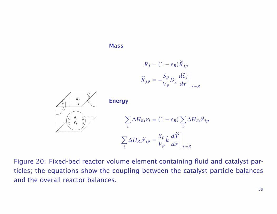
138
Rj
r iRj
ri
Mass
Rj = (1− εB)Rjp
Rjp = −SpVpDjdcjdr
∣∣∣∣∣r=R
Energy
∑i∆HRiri = (1− εB)
∑i∆HRir ip
∑i∆HRir ip =
SpVpkdTdr
∣∣∣∣∣r=R
Figure 20: Fixed-bed reactor volume element containing fluid and catalyst par-ticles; the equations show the coupling between the catalyst particle balancesand the overall reactor balances.
139
Summary
Equations 67–80 provide the full packed-bed reactor model given our as-sumptions.
We next examine several packed-bed reactor problems that can be solvedwithout solving this full set of equations.
Finally, we present an example that requires numerical solution of the fullset of equations.
140
First-order, isothermal fixed-bed reactor
Use the rate data presented in Example 7.1 to find the fixed-bed reactorvolume and the catalyst mass needed to convert 97% of A. The feed to the reactoris pure A at 1.5 atm at a rate of 12 mol/s. The 0.3 cm pellets are to be used,which leads to a bed density ρB = 0.6 g/cm3. Assume the reactor operatesisothermally at 450 K and that external mass-transfer limitations are negligible.
141
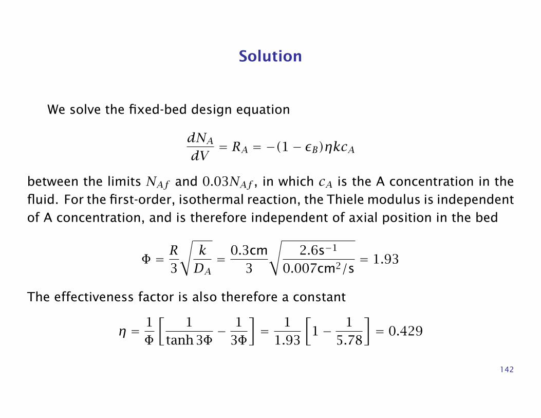
Solution
We solve the fixed-bed design equation
dNAdV
= RA = −(1− εB)ηkcA
between the limits NAf and 0.03NAf , in which cA is the A concentration in thefluid. For the first-order, isothermal reaction, the Thiele modulus is independentof A concentration, and is therefore independent of axial position in the bed
Φ = R3
√kDA= 0.3cm
3
√2.6s−1
0.007cm2/s= 1.93
The effectiveness factor is also therefore a constant
η = 1Φ
[1
tanh 3Φ− 1
3Φ
]= 1
1.93
[1− 1
5.78
]= 0.429
142
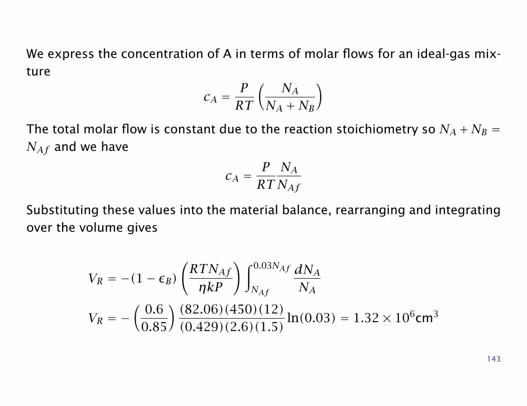
We express the concentration of A in terms of molar flows for an ideal-gas mix-ture
cA =PRT
(NA
NA +NB
)The total molar flow is constant due to the reaction stoichiometry so NA+NB =NAf and we have
cA =PRT
NANAf
Substituting these values into the material balance, rearranging and integratingover the volume gives
VR = −(1− εB)(RTNAfηkP
)∫ 0.03NAf
NAf
dNANA
VR = −(
0.60.85
)(82.06)(450)(12)(0.429)(2.6)(1.5)
ln(0.03) = 1.32× 106cm3
143
and
Wc = ρBVR =0.6
1000
(1.32× 10⁶
)= 789 kg
We see from this example that if the Thiele modulus and effectiveness factorsare constant, finding the size of a fixed-bed reactor is no more difficult thanfinding the size of a plug-flow reactor.
144
Mass-transfer limitations in a fixed-bed reactor
Reconsider Example given the following two values of the mass-transfercoefficient
km1 = 0.07 cm/s
km2 = 1.4 cm/s
145
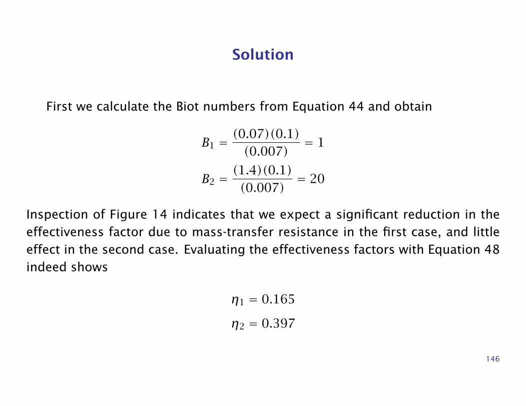
Solution
First we calculate the Biot numbers from Equation 44 and obtain
B1 =(0.07)(0.1)(0.007)
= 1
B2 =(1.4)(0.1)(0.007)
= 20
Inspection of Figure 14 indicates that we expect a significant reduction in theeffectiveness factor due to mass-transfer resistance in the first case, and littleeffect in the second case. Evaluating the effectiveness factors with Equation 48indeed shows
η1 = 0.165
η2 = 0.397
146
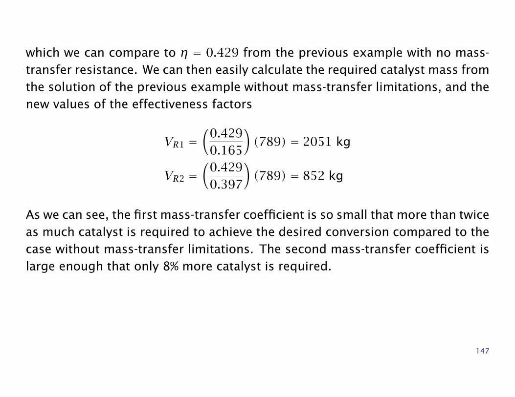
which we can compare to η = 0.429 from the previous example with no mass-transfer resistance. We can then easily calculate the required catalyst mass fromthe solution of the previous example without mass-transfer limitations, and thenew values of the effectiveness factors
VR1 =(
0.4290.165
)(789) = 2051 kg
VR2 =(
0.4290.397
)(789) = 852 kg
As we can see, the first mass-transfer coefficient is so small that more than twiceas much catalyst is required to achieve the desired conversion compared to thecase without mass-transfer limitations. The second mass-transfer coefficient islarge enough that only 8% more catalyst is required.
147
Second-order, isothermal fixed-bed reactor
Estimate the mass of catalyst required in an isothermal fixed-bed reactor forthe second-order, heterogeneous reaction.
Ak-→ B
r = kc2A k = 2.25× 105cm3/mol s
The gas feed consists of A and an inert, each with molar flowrate of 10 mol/s, thetotal pressure is 4.0 atm and the temperature is 550 K. The desired conversionof A is 75%. The catalyst is a spherical pellet with a radius of 0.45 cm. Thepellet density is ρp = 0.68 g/cm3 and the bed density is ρB = 0.60 g/cm3. Theeffective diffusivity of A is 0.008 cm2/s and may be assumed constant. You mayassume the fluid and pellet surface concentrations are equal.
148
Solution
We solve the fixed-bed design equation
dNAdV
= RA = −(1− εB)ηkc2A
NA(0) = NAf (81)
between the limits NAf and 0.25NAf . We again express the concentration of Ain terms of the molar flows
cA =PRT
(NA
NA +NB +NI
)
As in the previous example, the total molar flow is constant and we know its
149
value at the entrance to the reactor
NT = NAf +NBf +NIf = 2NAf
Therefore,
cA =PRT
NA2NAf
(82)
Next we use the definition of Φ for nth-order reactions given in Equation 35
Φ = R3
[(n+ 1)kcn−1
A2DA
]1/2
= R3
(n+ 1)k2DA
(PRT
NA2NAf
)n−11/2
(83)
Substituting in the parameter values gives
Φ = 9.17
(NA
2NAf
)1/2
(84)
150
For the second-order reaction, Equation 84 shows that Φ varies with the molarflow, which means Φ and η vary along the length of the reactor as NA decreases.We are asked to estimate the catalyst mass needed to achieve a conversion of Aequal to 75%. So for this particular example, Φ decreases from 6.49 to 3.24. Asshown in Figure 8, we can approximate the effectiveness factor for the second-order reaction using the analytical result for the first-order reaction, Equation 30,
η = 1Φ
[1
tanh 3Φ− 1
3Φ
](85)
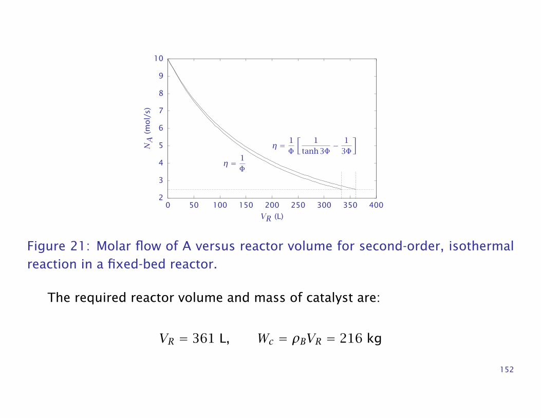
Summarizing so far, to compute NA versus VR, we solve one differential equa-tion, Equation 81, in which we use Equation 82 for cA, and Equations 84 and 85for Φ and η. We march in VR until NA = 0.25NAf . The solution to the differentialequation is shown in Figure 21.
151
2
3
4
5
6
7
8
9
10
0 50 100 150 200 250 300 350 400
NA
(mo
l/s)
η = 1Φ
η = 1Φ
[1
tanh 3Φ− 1
3Φ
]
VR (L)
Figure 21: Molar flow of A versus reactor volume for second-order, isothermalreaction in a fixed-bed reactor.
The required reactor volume and mass of catalyst are:
VR = 361 L, Wc = ρBVR = 216 kg
152
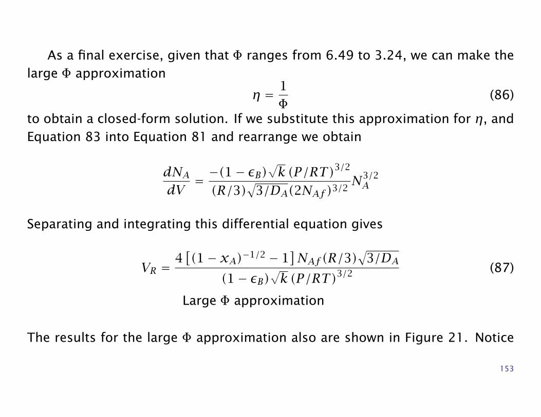
As a final exercise, given that Φ ranges from 6.49 to 3.24, we can make thelarge Φ approximation
η = 1Φ
(86)
to obtain a closed-form solution. If we substitute this approximation for η, andEquation 83 into Equation 81 and rearrange we obtain
dNAdV
= −(1− εB)√k (P/RT)3/2
(R/3)√
3/DA(2NAf)3/2N3/2A
Separating and integrating this differential equation gives
VR =4[(1− xA)−1/2 − 1
]NAf(R/3)
√3/DA
(1− εB)√k (P/RT)3/2
(87)
Large Φ approximation
The results for the large Φ approximation also are shown in Figure 21. Notice
153
from Figure 8 that we are slightly overestimating the value of η using Equa-tion 86, so we underestimate the required reactor volume. The reactor size andthe percent change in reactor size are
VR = 333 L, ∆ = −7.7%
Given that we have a result valid for all Φ that requires solving only a single differ-ential equation, one might question the value of this closed-form solution. Oneadvantage is purely practical. We may not have a computer available. Instruc-tors are usually thinking about in-class examination problems at this juncture.The other important advantage is insight. It is not readily apparent from the dif-ferential equation what would happen to the reactor size if we double the pelletsize, or halve the rate constant, for example. Equation 87, on the other hand,provides the solution’s dependence on all parameters. As shown in Figure 21the approximation error is small. Remember to check that the Thiele modulusis large for the entire tube length, however, before using Equation 87.
154
Hougen-Watson kinetics in a fixed-bed reactor
The following reaction converting CO to CO2 takes place in a catalytic, fixed-bed reactor operating isothermally at 838 K and 1.0 atm
CO+ 12
O2 -→ CO2 (88)
The following rate expression and parameters are adapted from a differentmodel given by Oh et al. [8]. The rate expression is assumed to be of theHougen-Watson form
r = kcCOcO2
1+KcCOmol/s cm3 pellet
155
The constants are provided below
k = 8.73× 10¹² exp(−13,500/T) cm3/mol s
K = 8.099× 10⁶ exp(409/T) cm3/mol
DCO = 0.0487 cm2/s
in which T is in Kelvin. The catalyst pellet radius is 0.1 cm. The feed to thereactor consists of 2 mol% CO, 10 mol% O2, zero CO2 and the remainder inerts.Find the reactor volume required to achieve 95% conversion of the CO.
156
Solution
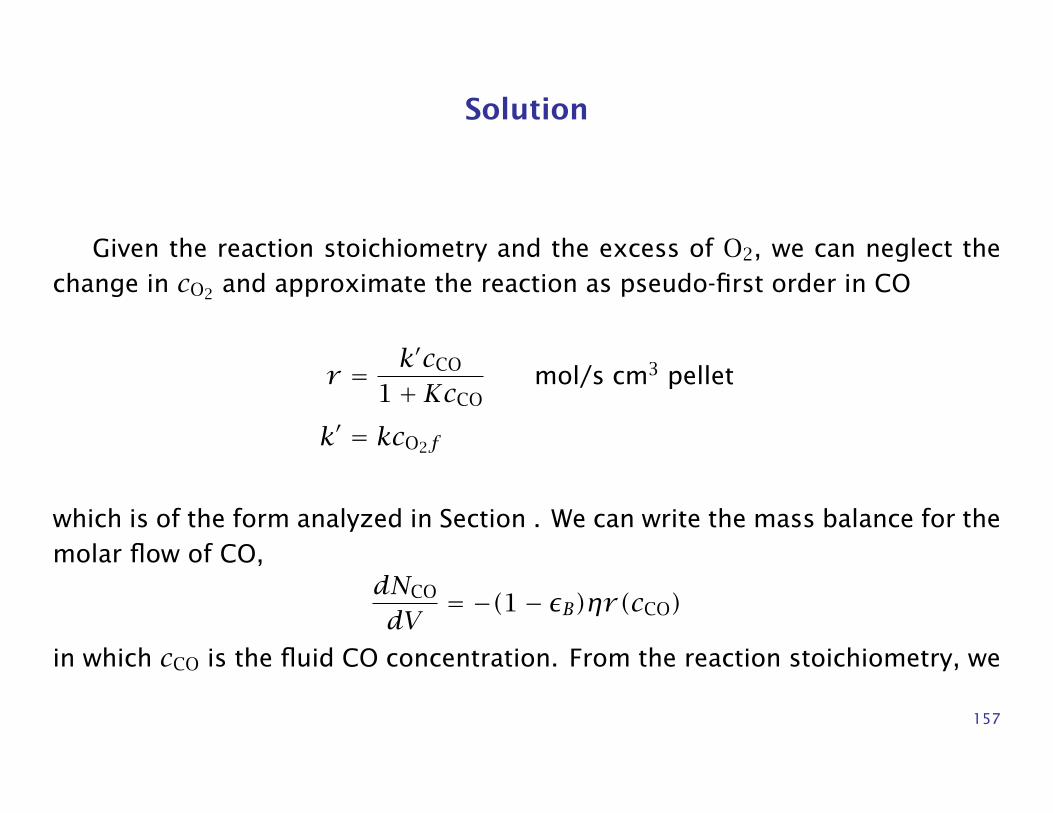
Given the reaction stoichiometry and the excess of O2, we can neglect thechange in cO2 and approximate the reaction as pseudo-first order in CO
r = k′cCO
1+KcCOmol/s cm3 pellet
k′ = kcO2f
which is of the form analyzed in Section . We can write the mass balance for themolar flow of CO,
dNCO
dV= −(1− εB)ηr(cCO)
in which cCO is the fluid CO concentration. From the reaction stoichiometry, we
157
can express the remaining molar flows in terms of NCO
NO2 = NO2f + 1/2(NCO −NCOf)
NCO2 = NCOf −NCO
N = NO2f + 1/2(NCO +NCOf)
The concentrations follow from the molar flows assuming an ideal-gas mixture
cj =PRTNjN
158
0
2.0× 10⁻⁶
4.0× 10⁻⁶
6.0× 10⁻⁶
8.0× 10⁻⁶
1.0× 10⁻⁵
1.2× 10⁻⁵
1.4× 10⁻⁵
0 50 100 150 200 250
O2
CO2
CO
c j(m
ol/
cm3
)
VR (cm3)
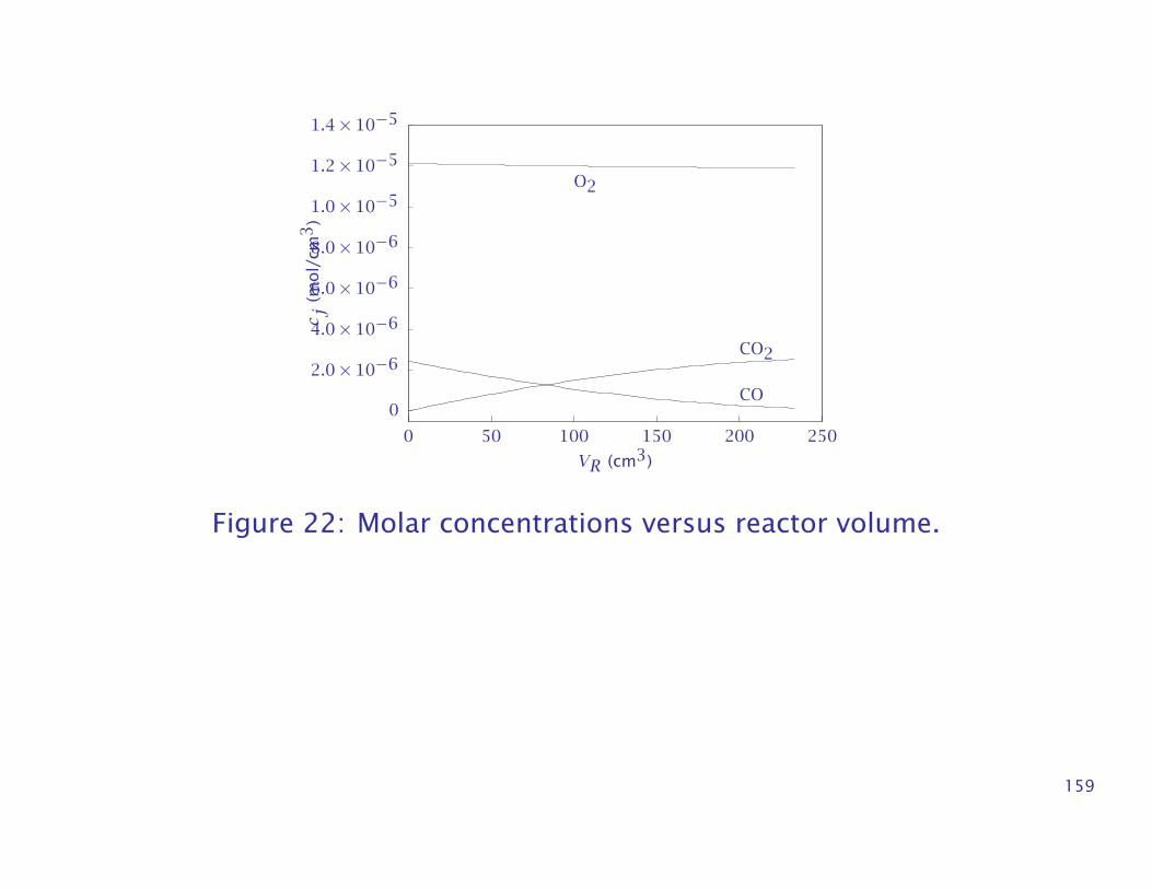
Figure 22: Molar concentrations versus reactor volume.
159
0
50
100
150
200
250
300
350
0 50 100 150 200 250
0
5
10
15
20
25
30
35
φ Φ
Φ φ
VR (cm3)
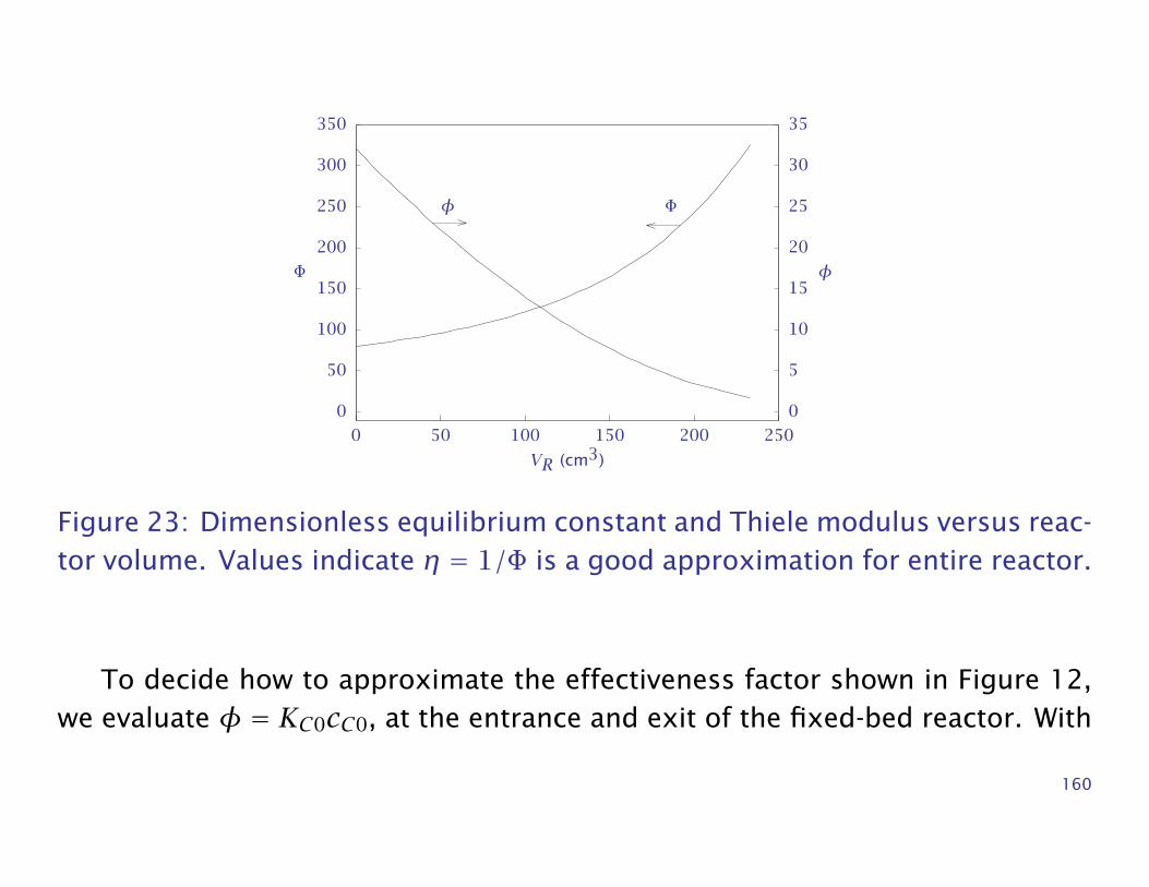
Figure 23: Dimensionless equilibrium constant and Thiele modulus versus reac-tor volume. Values indicate η = 1/Φ is a good approximation for entire reactor.
To decide how to approximate the effectiveness factor shown in Figure 12,we evaluate φ = KC0cC0, at the entrance and exit of the fixed-bed reactor. With
160
φ evaluated, we compute the Thiele modulus given in Equation 41 and obtain
φ = 32.0 Φ= 79.8, entrance
φ = 1.74 Φ = 326, exit
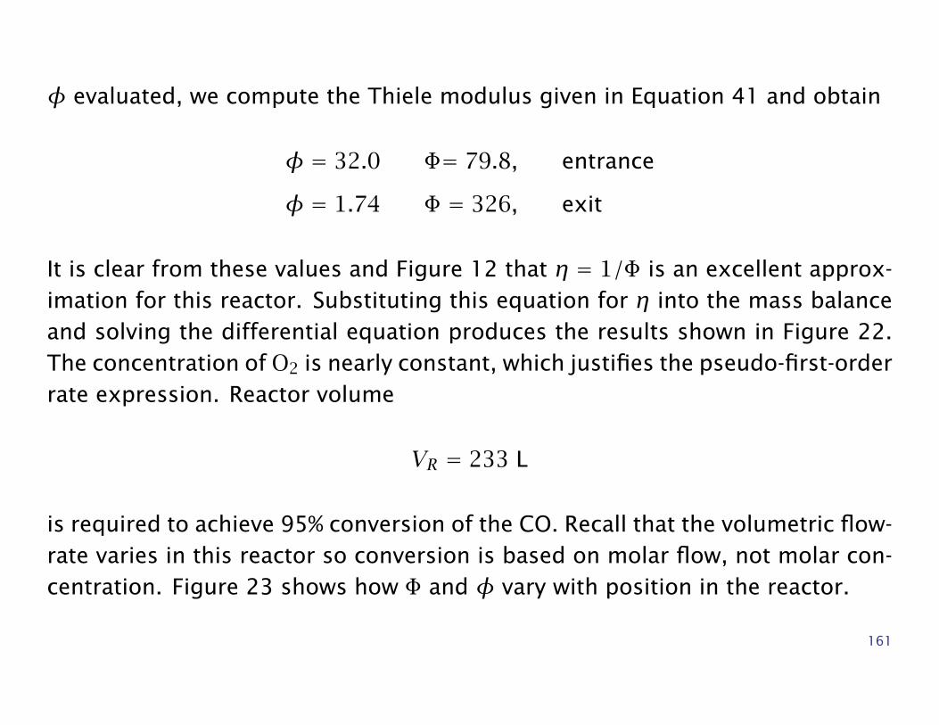
It is clear from these values and Figure 12 that η = 1/Φ is an excellent approx-imation for this reactor. Substituting this equation for η into the mass balanceand solving the differential equation produces the results shown in Figure 22.The concentration of O2 is nearly constant, which justifies the pseudo-first-orderrate expression. Reactor volume
VR = 233 L
is required to achieve 95% conversion of the CO. Recall that the volumetric flow-rate varies in this reactor so conversion is based on molar flow, not molar con-centration. Figure 23 shows how Φ and φ vary with position in the reactor.
161
In the previous examples, we have exploited the idea of an effectiveness fac-tor to reduce fixed-bed reactor models to the same form as plug-flow reactormodels. This approach is useful and solves several important cases, but thisapproach is also limited and can take us only so far. In the general case, wemust contend with multiple reactions that are not first order, nonconstant ther-mochemical properties, and nonisothermal behavior in the pellet and the fluid.For these cases, we have no alternative but to solve numerically for the temper-ature and species concentrations profiles in both the pellet and the bed. As afinal example, we compute the numerical solution to a problem of this type.
We use the collocation method to solve the next example, which involves fivespecies, two reactions with Hougen-Watson kinetics, both diffusion and exter-nal mass-transfer limitations, and nonconstant fluid temperature, pressure andvolumetric flowrate.
Evaluate the performance of the catalytic converter in converting CO andpropylene.
Determine the amount of catalyst required to convert 99.6% of the CO andpropylene.
The reaction chemistry and pellet mass-transfer parameters are given in Ta-ble 4.
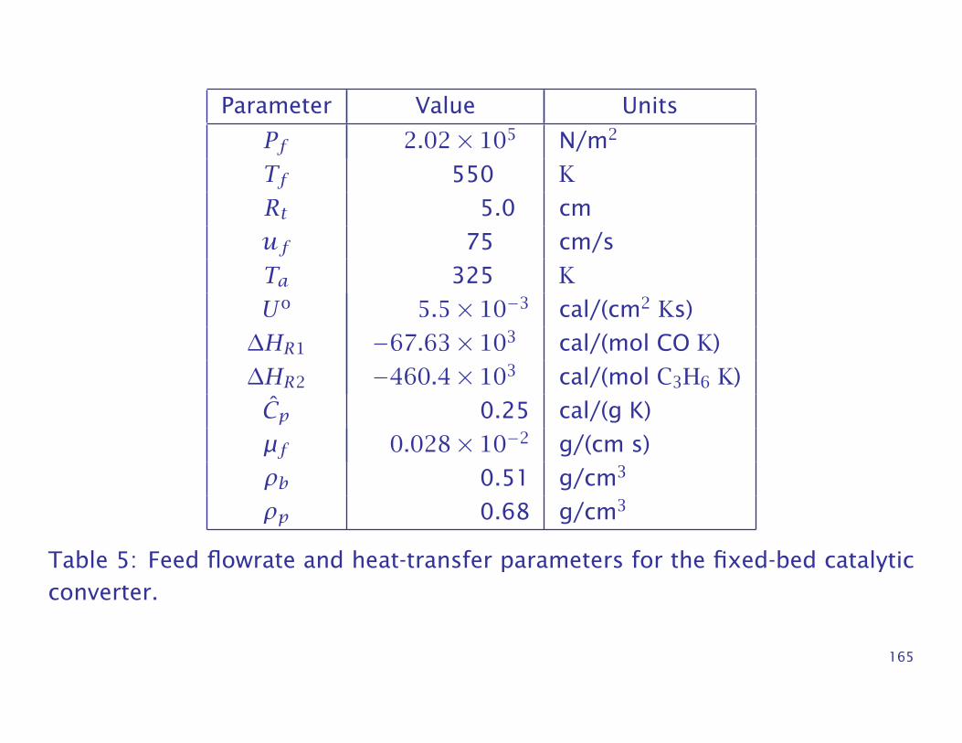
The feed conditions and heat-transfer parameters are given in Table 5.
163
Feed conditions and heat-transfer parameters
164
Parameter Value Units
Pf 2.02× 10⁵ N/m2
Tf 550 K
Rt 5.0 cm
uf 75 cm/s
Ta 325 K
Uo 5.5× 10⁻³ cal/(cm2 Ks)
∆HR1 −67.63× 10³ cal/(mol CO K)
∆HR2 −460.4× 10³ cal/(mol C3H6 K)
Cp 0.25 cal/(g K)
µf 0.028× 10⁻² g/(cm s)
ρb 0.51 g/cm3
ρp 0.68 g/cm3
Table 5: Feed flowrate and heat-transfer parameters for the fixed-bed catalyticconverter.
165
Solution
• The fluid balances govern the change in the fluid concentrations, temperatureand pressure.
• The pellet concentration profiles are solved with the collocation approach.
• The pellet and fluid concentrations are coupled through the mass-transferboundary condition.
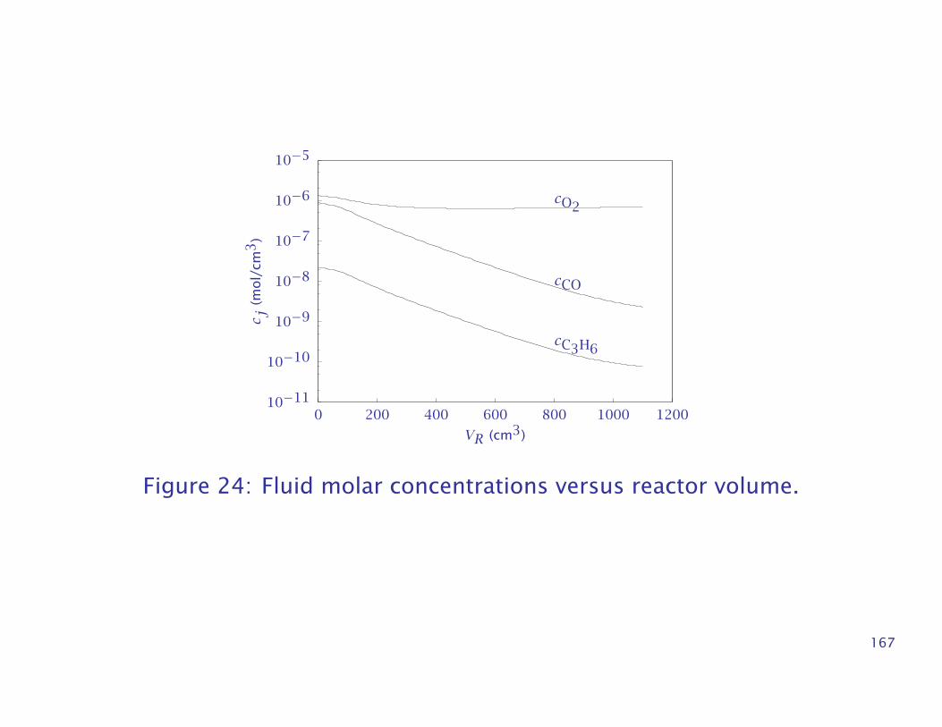
• The fluid concentrations are shown in Figure 24.
• A bed volume of 1098 cm3 is required to convert the CO and C3H6. Figure 24also shows that oxygen is in slight excess.
166
10−11
10−10
10−9
10−8
10−7
10−6
10−5
0 200 400 600 800 1000 1200
cO2
cCO
cC3H6
c j(m
ol/
cm3
)
VR (cm3)
Figure 24: Fluid molar concentrations versus reactor volume.
167
Solution (cont.)
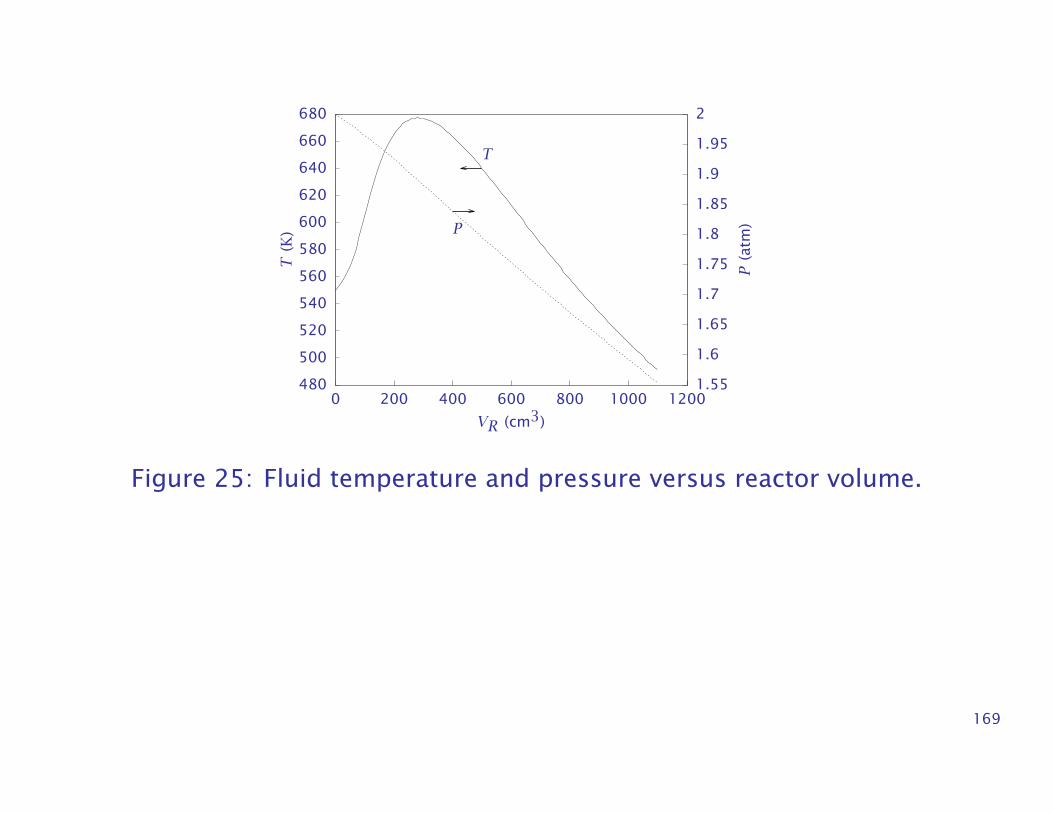
• The reactor temperature and pressure are shown in Figure 25.
The feed enters at 550 K, and the reactor experiences about a 130 K tem-perature rise while the reaction essentially completes; the heat losses thenreduce the temperature to less than 500 K by the exit.
• The pressure drops from the feed value of 2.0 atm to 1.55 atm at the exit.Notice the catalytic converter exit pressure of 1.55 atm must be large enoughto account for the remaining pressure drops in the tail pipe and muffler.
168
480
500
520
540
560
580
600
620
640
660
680
0 200 400 600 800 1000 12001.55
1.6
1.65
1.7
1.75
1.8
1.85
1.9
1.95
2
T(K
)
P(a
tm)
T
P
VR (cm3)
Figure 25: Fluid temperature and pressure versus reactor volume.
169
Solution (cont.)
• In Figures 26 and 27, the pellet CO concentration profile at several reactorpositions is displayed.
• We see that as the reactor heats up, the reaction rates become large and theCO is rapidly converted inside the pellet.
• By 490 cm3 in the reactor, the pellet exterior CO concentration has droppedby two orders of magnitude, and the profile inside the pellet has become verysteep.
• As the reactions go to completion and the heat losses cool the reactor, thereaction rates drop. At 890 cm3, the CO begins to diffuse back into the pellet.
170
• Finally, the profiles become much flatter near the exit of the reactor.
171
490900 890 990 1098
VR (cm3)
40
Ã Ä Å ÆÂÁÀ
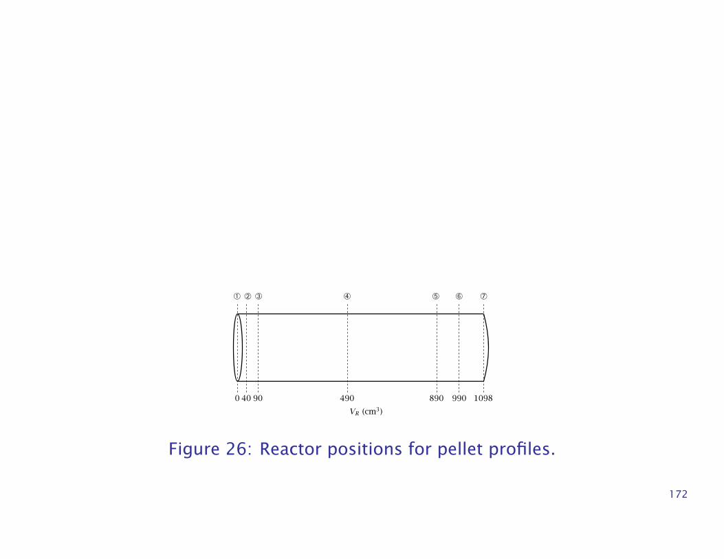
Figure 26: Reactor positions for pellet profiles.
172
10−15
10−14
10−13
10−12
10−11
10−10
10−9
10−8
10−7
10−6
0 0.05 0.1 0.15 0.175
À Á Â
ÃÄÅ
Æ
c CO
(mo
l/cm
3)
r (cm)
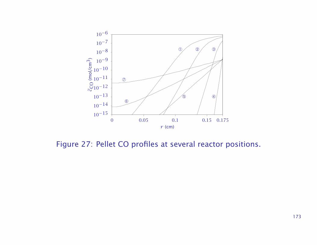
Figure 27: Pellet CO profiles at several reactor positions.
173
• It can be numerically challenging to calculate rapid changes and steep profilesinside the pellet.
• The good news, however, is that accurate pellet profiles are generally notrequired for an accurate calculation of the overall pellet reaction rate. Thereason is that when steep profiles are present, essentially all of the reactionoccurs in a thin shell near the pellet exterior.
• We can calculate accurately down to concentrations on the order of 10−15 asshown in Figure 27, and by that point, essentially zero reaction is occurring,and we can calculate an accurate overall pellet reaction rate.
• It is always a good idea to vary the numerical approximation in the pelletprofile, by changing the number of collocation points, to ensure convergencein the fluid profiles.
174
• Congratulations, we have finished the most difficult example in the text.
175
Summary
• This chapter treated the fixed-bed reactor, a tubular reactor packed with cat-alyst pellets.
• We started with a general overview of the transport and reaction events thattake place in the fixed-bed reactor: transport by convection in the fluid; dif-fusion inside the catalyst pores; and adsorption, reaction and desorption onthe catalyst surface.
• In order to simplify the model, we assumed an effective diffusivity could beused to describe diffusion in the catalyst particles.
• We next presented the general mass and energy balances for the catalystparticle.
176
Summary
• Next we solved a series of reaction-diffusion problems in a single catalystparticle. These included:
– Single reaction in an isothermal pellet. This case was further divided intoa number of special cases.∗ First-order, irreversible reaction in a spherical particle.∗ Reaction in a semi-infinite slab and cylindrical particle.∗ nth order, irreversible reaction.∗ Hougen-Watson rate expressions.∗ Particle with significant external mass-transfer resistance.
– Single reaction in a nonisothermal pellet.– Multiple reactions.
177
Summary
• For the single-reaction cases, we found a dimensionless number, the Thielemodulus (Φ), which measures the rate of production divided by the rate ofdiffusion of some component.
• We summarized the production rate using the effectiveness factor (η), theratio of actual rate to rate evaluated at the pellet exterior surface conditions.
• For the single-reaction, nonisothermal problem, we solved the so-calledWeisz-Hicks problem, and determined the temperature and concentrationprofiles within the pellet. We showed the effectiveness factor can be greaterthan unity for this case. Multiple steady-state solutions also are possible forthis problem.
178
• For complex reactions involving many species, we must solve numericallythe complete reaction-diffusion problem. These problems are challengingbecause of the steep pellet profiles that are possible.
179
Summary
• Finally, we showed several ways to couple the mass and energy balances overthe fluid flowing through a fixed-bed reactor to the balances within the pellet.
• For simple reaction mechanisms, we were still able to use the effectivenessfactor approach to solve the fixed-bed reactor problem.
• For complex mechanisms, we solved numerically the full problem given inEquations 67–80.
• We solved the reaction-diffusion problem in the pellet coupled to the massand energy balances for the fluid, and we used the Ergun equation to calculatethe pressure in the fluid.
180
Notation
a characteristic pellet length, Vp/SpAc reactor cross-sectional area
B Biot number for external mass transfer
c constant for the BET isotherm
cj concentration of species jcjs concentration of species j at the catalyst surface
c dimensionless pellet concentration
cm total number of active surface sites
DAB binary diffusion coefficient
Dj effective diffusion coefficient for species jDjK Knudsen diffusion coefficient for species jDjm diffusion coefficient for species j in the mixture
Dp pellet diameter
181
Ediff activation energy for diffusion
Eobs experimental activation energy
Erxn intrinsic activation energy for the reaction
∆HRi heat of reaction iIj rate of transport of species j into a pellet
I0 modified Bessel function of the first kind, zero order
I1 modified Bessel function of the first kind, first order
ke effective thermal conductivity of the pellet
kmj mass-transfer coefficient for species jkn nth-order reaction rate constant
L pore length
Mj molecular weight of species jnr number of reactions in the reaction network
N total molar flow,∑jNj
Nj molar flow of species jP pressure
Q volumetric flowrate
182
r radial coordinate in catalyst particle
ra average pore radius
ri rate of reaction i per unit reactor volume
robs observed (or experimental) rate of reaction in the pellet
rip total rate of reaction i per unit catalyst volume
r dimensionless radial coordinate
R spherical pellet radius
R gas constant
Rj production rate of species jRjf production rate of species j at bulk fluid conditions
Rjp total production rate of species j per unit catalyst volume
Rjs production rate of species j at the pellet surface conditions
Sg BET area per gram of catalyst
Sp external surface area of the catalyst pellet
T temperature
Tf bulk fluid temperature
Ts pellet surface temperature
183
Uo overall heat-transfer coefficient
v volume of gas adsorbed in the BET isotherm
vm volume of gas corresponding to an adsorbed monolayer
V reactor volume coordinate
Vg pellet void volume per gram of catalyst
Vp volume of the catalyst pellet
VR reactor volume
Wc total mass of catalyst in the reactor
yj mole fraction of species jz position coordinate in a slab
ε porosity of the catalyst pellet
εB fixed-bed porosity or void fraction
η effectiveness factor
λ mean free path
µf bulk fluid density
νij stoichiometric number for the jth species in the ith reaction
ξ integral of a diffusing species over a bounding surface
184
ρ bulk fluid density
ρB reactor bed density
ρp overall catalyst pellet density
ρs catalyst solid-phase density
σ hard sphere collision radius
τ tortuosity factor
Φ Thiele modulus
ΩD,AB dimensionless function of temperature and the intermolecular potential field for
one molecule of A and one molecule of B
185
References
[1] R. Aris. A normalization for the Thiele modulus. Ind. Eng. Chem. Fundam.,4:227, 1965.
[2] R. Aris. The Mathematical Theory of Diffusion and Reaction in PermeableCatalysts. Volume I: The Theory of the Steady State. Clarendon Press, Ox-ford, 1975.
[3] R. B. Bird, W. E. Stewart, and E. N. Lightfoot. Notes on Transport Phenom-ena. John Wiley & Sons, New York, 1958.
[4] K. B. Bischoff. Effectiveness factors for general reaction rate forms. AIChEJ., 11:351, 1965.
[5] S. Brunauer, P. H. Emmett, and E. Teller. Adsorption of gases in multimolec-ular layers. J. Am. Chem. Soc., 60:309–319, 1938.
186
[6] S. Ergun. Fluid flow through packed columns. Chem. Eng. Prog., 48(2):89–94, 1952.
[7] B. C. Gates. Catalytic Chemistry. John Wiley & Sons, New York, 1992.
[8] S. H. Oh, J. C. Cavendish, and L. L. Hegedus. Mathematical modeling ofcatalytic converter lightoff: Single-pellet studies. AIChE J., 26(6):935–943,1980.
[9] C. J. Pereira, J. B. Wang, and A. Varma. A justification of the internal iso-thermal model for gas-solid catalytic reactions. AIChE J., 25(6):1036–1043,1979.
[10] E. E. Petersen. A general criterion for diffusion influenced chemical reac-tions in porous solids. Chem. Eng. Sci., 20:587–591, 1965.
187
[11] E. W. Thiele. Relation between catalytic activity and size of particle. Ind.Eng. Chem., 31(7):916–920, 1939.
[12] P. B. Weisz. Zeolites - new horizons in catalysts. Chem. Tech., 3:498, 1973.
[13] P. B. Weisz and J. S. Hicks. The behaviour of porous catalyst particles in viewof internal mass and heat diffusion effects. Chem. Eng. Sci., 17:265–275,1962.