Fixed mesh methods in computational mechanics

Ramon Codina and Joan Baiges

May 12, 2010

Abstract

In many coupled problems of practical interest the domain ofat least one of the prob-lems evolves in time. The Arbitrary Eulerian Lagrangian (ALE) approach is a toolvery often employed to cope with this domain motion. However, in this work we aimat describing numerical techniques that allow us to use a fixed mesh for the approxi-mation of moving boundary problems, particularly using thefinite element approach.This type of formulations is often termed embedded or immersed boundary methods.Emphasis will be put in describing a particular version of the ALE formulation usingfixed meshes that we have developed, and that we call fixed-mesh ALE method (FM-ALE). Methods able to deal with fixed meshes are closely linked to the approximateimposition of boundary conditions. Some possibilities to do this approximation arealso described.

Keywords: moving domains, fixed mesh methods, ALE, approximate boundary con-ditions

1 Introduction

In the classical ALE approach to solve problems in computational fluid dynamics, themesh in which the computational domain is discretized is deformed (see for example[16, 33, 35]). This is done according to a prescribed motion of part of its boundary,which is transmitted to the interior nodes in a way as smooth as possible so as to avoidmesh distortion. The FM-ALE formulation has a different motivation. Instead ofassuming that the computational domain is defined by the meshboundary, we assumethat there is a function that defines the boundary of the domain where the flow takesplace. We will refer to it as the boundary function. It may be given, for example, bythe shape of a body that moves within the fluid, or it may need tobe computed, as inthe case of level set functions. It may be also defined discretely, by a set of points.When this boundary function moves, the flow domain changes, and that must be takeninto account at the moment of writing the conservation equations that govern the flow,

1

which need to be cast in the ALE format. However, our purpose here is to explain howto use always a background fixed mesh. A review of the method will be presented.

Other possibilities to use a single grid in the whole simulation can be found inthe literature, each one having advantages and drawbacks. They were designed asan alternative to body fitted meshes and can be divided into two main groups, corre-sponding in fact to two ways of prescribing the boundary conditions on the movingboundary [13]:

• Force term. The interaction of the fluid and the solid is takeninto accountthrough a force term, which appears either in the strong or inthe weak formof the flow equations. Among this type of methods, let us cite for example theImmersed Boundary method as a variant of the Penalty method,where punctualforces are added to the momentum equation, and the Fictitious Domain method,where the solid boundary conditions are imposed through a Lagrange multiplier.

• Approximate boundary conditions. Instead of adding a forceterm, these meth-ods impose the boundary conditions in an approximate way once the discretiza-tion has been carried out, either by modifying the differential operators near theinterface (in finite differences) or by modifying the unknowns near the interface.

The Immersed Boundary Method in its original form [48] consists in adding punctualpenalty forces in the domain boundary so that the boundary conditions are fulfilled.The forces are computed from a fluid-structure (elastic) interaction problem at the in-terface. The method is first order accurate even if second order approximation schemesare used, although formal second order accuracy has been reported in [40]. The morerecent Immersed Interface Method achieves higher order accuracy by avoiding the useof the Dirac delta distribution to define the forcing terms (see [41,42,56]).

The Penalty method is similar to the previous one in the sensethat a force term isadded to the momentum equations. The difference is due to thefact that the penaltyparameter is not computed from a fluid-structure interaction as in the original im-mersed boundary method, but it is simply required to be largeenough to enforce theboundary conditions approximately [53].

Another approach is the use of Lagrange multipliers to enforce the boundary con-ditions. However, the finite element subspaces for the bulk and Lagrange multiplierfields must satisfy the classical inf-sup condition, which usually leads to the need forstabilization. Moreover, additional degrees of freedom must be added to the problem.The use of Lagrange multipliers is the basis of the Fictitious Domain Method [23,26].

Another possibility for imposing boundary conditions is the use of preexisting gridnodes to impose boundary conditions. This is the case of the FM-ALE method, whichapplies a variant of the ALE method to a fixed mesh strategy [2,14, 15, 32] and thehybrid Cartesian/immersed boundary methods for Cartesiangrids [19,45,57].

Most of these methods have been well tested in the literaturefor both steady andmoving interfaces. Generally, the last case is treated by applying directly the formerat each time step. In this work we review all these formulations from a unified pointof view.

The chapter is organized as follows. In Section 2 we present ageneral overviewof the physical problem and equations with which fixed mesh methods have to deal,which we particularize for the finite element method. In Section 3 we describe sev-eral existing possibilities for imposing Dirichlet boundary conditions in fixed meshmethods. Imposing Dirichlet boundary conditions is an essential ingredient of anyfixed grid strategy, and it is very closely related to treatment of the ALE equationsin moving domains. In Section 4 we present different possibilities to treat movingsubdomains with fixed-mesh strategies. Finally, a summary of the methods describedcloses the chapter in Section 5.

2 Problem statement

In this section we state the continuous problem to be solved.Fixed mesh methodsapplied to problems in moving domains appear in different applications. However, tofix ideas we will concentrate our developments to fluid-structure interaction problemsin which the solid (structure) either deforms or has rigid body motions. The fluiddomain will therefore change in time. Our main interest is todescribe strategies ableto deal with this situation. A more detailed description of the problem can be foundin [2,14].

2.1 Flow equations

Let us consider a regionΩ0 ⊂ Rd (d = 2, 3) where a flow will take place during a time

interval [0, T ]. However, we consider the case in which the fluid at timet occupiesonly a subdomainΩ(t) ⊂ Ω0 (note in particular thatΩ(0) ⊂ Ω0). Suppose also thatthe boundary ofΩ(t) is defined by part of∂Ω0 and a moving boundary that we callΓfree(t) = ∂Ω(t) \ ∂Ω0 ∩ ∂Ω(t). This moving part of∂Ω(t) may correspond to theboundary of a moving solid immersed in the fluid.

In order to cope with the time-dependency ofΩ(t), we may use the ALE approach,with the particular feature of considering a variable definition of the domain velocity.Let χt be a family of invertible mappings, which for allt ∈ [0, T ] map a pointX ∈Ω(0) to a pointx = χt(X) ∈ Ω(t), with χ0 = I, the identity. Ifχt is given bythe motion of the particles, the resulting formulation would be Lagrangian, whereas ifχt = I for all t, Ω(t) = Ω(0) and the formulation would be Eulerian.

Let nowt′ ∈ [0, T ], with t′ ≤ t, and consider the mapping

χt,t′ : Ω(t′) −→ Ω(t)

x′ 7→ x = χt χ−1

t′ (x′).

Given a functionf : Ω(t) × (0, T ) −→ R we define

∂f

∂t

∣

∣

∣

∣

x′

(x, t) :=∂(f χt,t′)

∂t(x′, t), x ∈ Ω(t), x′ ∈ Ω(t′).

In particular, the domain velocity taking as a reference thecoordinates ofΩ(t′) isgiven by

udom :=∂x

∂t

∣

∣

∣

∣

x′

(x, t). (1)

The incompressible Navier-Stokes formulated inΩ(t), accounting also for the mo-tion of this domain, can be written as follows: find a velocityu : Ω(t)×(0, T ) −→ R

d

and a pressurep : Ω(t) × (0, T ) −→ R such that

ρ

[

∂u

∂t

∣

∣

∣

∣

x′

(x, t) + (u − udom) · ∇u

]

−∇ · (2µ∇Su) + ∇p = ρf , (2)

∇ · u = 0, (3)

where∇Su is the symmetrical part of the velocity gradient,ρ is the fluid density,µ isthe viscosity andf is the vector of body forces.

Initial and boundary conditions have to be appended to problem (2)-(3). Theboundary conditions onΓfree(t) can be of two different types: a)p (or the normalstress) given,u unknown onΓfree; b) u given,p (or the normal stress) unknown onΓfree. On the rest of the boundary ofΩ(t) the usual boundary conditions can be con-sidered. In general, we consider these boundary conditionsof the form

u = u onΓD,

n · σ = t onΓN ,

wheren is the external normal to the boundary,σ = −pI + 2µ∇Su is the Cauchystress tensor andu andt are the given boundary data. The components of the boundaryΓD andΓN are obviously disjoint and such thatΓD ∪ ΓN = ∂Ω, and therefore time-dependent.

We will also introduce the time and spatial discretization of the problem since someof the methods we will describe are directly applied to the discrete problem. We willfocus in the finite element method, although other possibilities are obviously possible.

2.1.1 The time-discrete problem

Let us start introducing some notation. Consider a uniform partition of [0, T ] into Ntime intervals of lengthδt. Let us denote byfn the approximation of a time dependentfunctionf at time leveltn = nδt. We will also denote

δfn+1 = fn+1 − fn,

δtfn+1 =

fn+1 − fn

δt,

fn+θ = θfn+1 + (1 − θ)fn, θ ∈ [1/2, 1].

Suppose we are given a computational domain at timetn, with spatial coordinateslabeledxn, andun and pn are known in this domain. The velocityun+1 and thepressurepn+1 can then be found as the solution to the problem

ρ[

δtun+1

∣

∣

xn

+ (un+θ − un+θdom

) · ∇un+θ]

−∇ · (2µ∇Sun+θ) + ∇pn+1 = ρfn+1,

(4)

∇ · un+θ = 0, (5)

where nowδtun+1|

xn = (un+1(x) − un(xn))/δt, beingx = χtn+θ,tn(xn) the spatial

coordinates inΩ(tn+θ). The domain velocity given by (1), withx′ = xn, is approxi-mated as

un+θdom

=1

θδt

(

χtn+θ,tn(xn) − xn)

. (6)

2.1.2 The fully discrete problem

The next step is to consider the spatial discretization of problem (4)-(5). As for thetime discretization, different options are possible. For the sake of conciseness, here wesimply describe the straight-forward Galerkin finite element formulation, even thoughthere are instabilities that might appear due to dominant convective term or incompat-ible velocity-pressure interpolations. In order to overcome these numerical problemsof the standard Galerkin method, a stabilized finite elementformulation can be ap-plied. The formulation we use is presented in [11]. It is based on the subgrid scaleconcept introduced in [34], although when linear elements are used it reduces to theGalerkin/least-squares method described for example in [18].

Let Ωen+1 be a finite element partition of the domainΩ(tn+1), with index eranging from 1 to the number of elementsnel (which may be different at different timesteps). We denote with a subscripth the finite element approximation to the unknownfunctions, and byvh and qh the velocity and pressure test functions associated toΩen+1, respectively.

The finite element discretized method consists of findingun+1

h andpn+1

h such that∫

Ω

vh · ρ δtun+1

∣

∣

xn

+

∫

Ω

2∇Svh : µ∇Sun+θ

+

∫

Ω

vh · (ρ (un+θ − un+θdom

) · ∇un+θ) −

∫

Ω

pn+1

h ∇ · vh

=

∫

Ω

vh · fn+θ, (7)

∫

Ω

qh∇ · un+θh = 0. (8)

2.2 Solid body equations

Let us now consider the solid body domainΩs(t) ⊂ Ω0 , which also evolves in time.The solid mechanics problem formulated in a purely Lagrangian approach inΩs(t)

can be written as follows:

ρs

d2d

dt2= ∇ · σs + ρsb, (9)

ρsJ = ρs0, (10)

whereρs is the solid density,d is the displacement vector,σs is the Cauchy stresstensor,b is the vector of body forces and

F =∂x

∂X, J = det(F ).

For linear elastic isotropic materials we haveσs = λs(∇·d)I+2µs∇sd. Rigid bodies

could be treated as well in the methods to be described in the following.

The time discretization and finite element approximation ofthe above equations isstandard. We omit the details, which can be found for examplein [2].

3 Approximate imposition of boundary conditions

3.1 Motivation

As indicated previously, moving domain methods on fixed meshes are closely linkedto methods to approximate boundary conditions on non-matching meshes, since thelatter are a crucial ingredient of the former. For example, let us consider a fluid-structure interaction problem as described above. A classical way to proceed is tosolve equations (7)-(8) coupled with the discretized version of equations (9)-(10) inan iterative manner, using the continuity of velocities andstresses on the interfaceboundary as transmission conditions between the fluid and the solid. In order to havea stable scheme, stress conditions need to be applied to the solid (transmitting thestresses exerted by the fluid) and velocity (Dirichlet) conditions to the fluid (fixingthe motion of the boundary of the fluid domain by the motion obtained in the solid).The key point is precisely the prescription of these conditions on meshes that, as timeevolves, will not match the flow domain. We concentrate now onthe description ofmethods to treat this problem, which can be stated for stationary problems as well.

3.2 Problem setting

Let us now focus in the solution of the flow problem, for which we will use a non-matching finite element discretization. The ideas to be presented are extendable toother numerical formulations and other physical problems.However, some of thedifficulties we shall mention are characteristic of flow problems. Likewise, we willconsider general non-structured meshes, the application to Cartesian meshes beingobvious.

An issue of special relevance when using non-matching gridsis the imposition ofDirichlet boundary conditions. Let us describe the problemto be solved. Consider the

situation depicted in Fig. 1. A domainΩ ⊂ Rd, d = 2, 3, with boundaryΓ = ∂Ω (red

curve in Fig. 1), is covered by a mesh that occupies a domainΩh = Ωin ∪ ΩΓ, whereΩin ⊂ Ω is formed by the elements interior toΩ andΩΓ is formed by a set of elementscut byΓ. In turn, let us splitΩΓ = ΩΓ,in ∪ΩΓ,out, whereΩΓ,in = Ω ∩ΩΓ andΩΓ,out isthe interior ofΩΓ \ ΩΓ,in. Note thatΩ = Ωin ∪ ΩΓ,in. For simplicity, we will assumethat the intersection ofΓ with the element domains is a piecewise polynomial curve(in 2D) or surface (in 3D) of the same order as the finite element interpolation.

Suppose we want to solve a boundary value problem for the unknownu in Ω withthe mesh ofΩh already created and boundary conditionsu = u on Γ. The obviouschoice would be:

• Obtain the nodes ofΓ (circles in Fig. 1) from the intersection with the elementedges.

• Split the elements ofΩΓ,in so as to obtain a grid matching the boundaryΓ.

• Prescribe the boundary conditionuh = u in the classical way, whereuh denotesthe approximate solution.

This strategy leads to a local remeshing close toΓ that is involved from the compu-tational point of view. Obviously, the implementation of the strategy described is verysimple for unstructured simplicial meshes, but it is not so easy if one wants to use otherelement shapes and, definitely, prevents from using Cartesian meshes. Moreover, ifthe boundaryΓ evolves in time (a situation considered later) the number ofdegrees offreedom changes at each time instant, thus modifying the structure and sparsivity ofthe matrix of the final algebraic system. This is clearly an inconvenience even whenusing unstructured simplicial meshes. There are several methods for imposing bound-ary conditions which avoid the need for locally remeshing. Some of these methodsare described next.

3.3 Immersed boundary method

The immersed boundary method was introduced in 1972 by C. Peskin (see [39, 48]and [49] for an overview), and since then it has been widely used to simulate fluid-structure interaction problems in moving domains. The key point of the immersedboundary method is how Dirichlet boundary conditions are imposed: in the immersedboundary method boundary conditions are imposed through the introduction of a forcein the momentum equation. In principle this force is introduced only in the fluid-solidinterface by means of a Dirac-delta function, but in practice this function has to beextended to the nodes surrounding the interface due to the discrete nature of finiteelement meshes, and the Dirac-delta function is smoothed.

Suppose that the interface is represented by a set of Lagrangian points of coordi-natesxΓ,i, i = 1, 2, ..., P (points on the red curve in Fig. 1), which typically corre-spond to nodes in the Lagrangian solid body mesh, and that theforce to be added is

Figure 1: Setting

elastic. If the interface is considered a membrane, it should be computed from the cou-pling of the membrane with the fluid, and this is what is described for example in [49].However, a simpler option, often used in the applications, is to consider this force asproportional to the deviation of the boundary value of the velocity to the boundarycondition, in a spring-like model. Ifk is the constant of proportionality, the punc-tual force introduced by the immersed boundary method applied to the Navier-Stokesequations would be of the form

f =

P∑

i=1

k(u − u)δ(|x − xΓ,i|),

where summation extends to all nodes representing the boundary. This force, whensmoothed and introduced in the weak form of the problem yields the right-hand-sideterm

∫

Ω

vh · f =

∫

Ω

vh ·

P∑

i=1

k(u − u)δ(|x − xΓ,i|).

Theelastic/penaltyconstantk has to be large enough to guarantee that boundary con-ditions are strongly enough imposed, andδ is the smoothed Dirac-delta function whichcontrols the extent of the applied force.

In the continuous problem,k would be unbounded, and the Dirac-delta functionwould not be smoothed at all. However, using very large values for k and very sharpδ functions highly ill-conditions the discrete system of equations to be solved, whichis the reason for the smoothing. Note that this force extendsnot only over the fluid-solid interface, but over the whole computational domain and needs to be integrated.

However, theδ function limits its extent to one or two layers of nodes at each side ofthe interface. The immersed boundary method is qualified to be a diffusive methodin [44]. The reason stems from the discretization of the Dirac delta function which hasa finite support. Based on the same coupling principle, Wang and Liu [54] devised theExtended Immersed Boundary method to allow volumetric deformation of the elasticsolid.

3.4 Penalty methods and Nitsche’s method

Penalty methods are similar to Peskin’s methods in that theyintroduce a force to im-pose boundary conditions. The main difference is the definition of this force. Whilein the immersed boundary method this force is many times understood as an elasticspring, in penalty methods the nature of the force is purely numerical, and it evendepends on the discretization through a parameter which represents the element size.Moreover, the extent of the penalty force in penalty methodsis only over the interfacesurface and not over the whole computational domain. The expression for the penaltyforce is:

f =α

h(u − u),

which introduced in the discrete weak form of the problem yields∫

Γ

vh · f =

∫

Γ

vh ·α

h(uh − u), (11)

whereα is the penalty parameter andh is the element size. The largerα is the strongerthe boundary conditions are imposed, but also the more ill-conditioned the resultingsystem of equations becomes. Note that, unlike in the immersed boundary method,the integral extends only over the contour of the domain.

Nitsche’s method can be understood as an improvement of the original penaltymethod. If the penalty forces (11) are added, there is no reason why the test functionassociated to the boundary nodes must vanish, and thereforethis contribution must beaccounted for. If this is not done, a poor approximation of the unknowns close to theinterface is obtained, even if the boundary condition is well approximated.

If we define the operator

σ(v, q) := −2n · µ∇Sv + qn,

the term to be added to the right-hand-side of (7) is

−

∫

Γ

vh · σ(uh, ph) +

∫

Γ

vh ·α

h(uh − u). (12)

Of course, terms involvinguh andph should be moved to the left-hand-side (LHS) of(7), since they contribute to the system matrix. The problemwith (12) is that it yieldsa non-symmetric problem, even in the Stokes case. In order toavoid this, the Dirichlet

conditionu = u is weighted byσ(vh, qh). Thus, instead of adding only (11) to theLHS of (7), the method consists in adding

−

∫

Γ

vh · σ(uh, ph) −

∫

Γ

uh · σ(vh, qh) +

∫

Γ

u · σ(vh, qh) +

∫

Γ

vh ·α

h(uh − u).

(13)

Again, terms involvinguh andph should be moved to the LHS of (7). The resultingproblem is symmetric if the Stokes problem is considered. Let us remark that both in(11) and (13) it is important to evaluate the unknowns at the time step of consideration,since explicit treatments are usually highly unstable. When added to (7), the naturalchoice is to evaluate (11) and (13) atn + θ.

Nitsche’s method was proposed for the Poisson problem and analyzed in this case.It can be shown that the higher the value ofα, the better the approximation to theboundary condition at the expense of a poorer approximationto the differential equa-tion. However, for any value ofα it is possible to show that the method is stable andoptimally convergent. See [37] for a proof, including more general boundary con-ditions than used here (although for Poisson’s problem). The good performance ofNitsche’s method has been exploited also in other contexts,such as the imposition ofboundary conditions for discontinuous finite element approximations (see the originalwork in [1] and the extension in [29], for example), the imposition of transmissionconditions in domain decomposition with non-matching grids (as in [4, 28], amongmany others) or also in some stabilized finite element methods for which this methodfits nicely [8].

3.5 Lagrange multiplier techniques

Another possibility to enforce boundary conditions, whichdoes not involve a largepenalty or elastic terms, is the use of Lagrange multipliers. Lagrange multipliers con-sist of adding new equations to the global system of equations that enforce the bound-ary conditions. New unknowns (the Lagrange multipliers) need also to be added to theproblem. The main advantage of this procedure is that the system does not become ill-conditioned. On the other hand, the system of equations becomes larger, and the spacefor the Lagrange multipliers has to be carefully chosen so that the final formulation isstable (or stabilization techniques should be used, see forexample [3,17]).

Using Lagrange multipliers to impose boundary conditions to the Navier-Stokesequations consists of adding the term

∫

Γ

vh · λh

to the LHS of the momentum equation (7) and to add the new equations for the La-grange multipliers

∫

Γ

γh · (uh − u) = 0,

whereλh are the Lagrange multipliers of the finite element problem and γh theirassociated test functions. Note that the Lagrange multipliers contribution to the mo-mentum equation corresponds exactly to that of the stressesthrough the boundary, thatis to say,λ = σ(u, p) for the continuous problem. In the discrete case, their intro-duction avoids the need for post-processing the stresses inorder to compute the forcesexerted by the fluid on the solid body.

The Lagrange multiplier technique for imposing boundary conditions is associ-ated to thefictitious domainmethod, in which the flow problem is solved over all thecomputational domain, including the region occupied by thesolid body [22, 24]. Wedescribe it later as a method to treat problems in moving domains.

3.6 Minimization of boundary errors with external degrees offreedom

Another possibility in order to avoid the ill-conditioningdue to penalty terms (whichappears in the immersed boundary and penalty methods), and the need of adding newdegrees of freedom to the system of equations (which appearsif Lagrange multipliersare used) is to use currently existing degrees of freedom in order to enforce boundaryconditions. This involves replacing momentum equations innodes adjacent to thefluid-solid interface with the equations that enforce boundary conditions.

There are several methods which use pre-existing degrees offreedom in order toenforce boundary conditions but we will focus here in our ownapproach to the prob-lem. We summarize next the strategy proposed in [12] to prescribe Dirichlet boundaryconditions on a generic immersed boundary, that we denote asbefore byΓ.

Let uh be the unknown solution of a problem posed inΩ ⊂ Ω0 for which we wantto prescribe a condition onΓ. Let ΩΓ be the set of elements cut byΓ, which is split asΩΓ = ΩΓ,in ∪ ΩΓ,out, whereΩΓ,in = Ω ∩ ΩΓ andΩΓ,out is the interior ofΩΓ \ ΩΓ,in.Let alsoΩin be such thatΩ = Ωin ∪ ΩΓ,in. For simplicity, we will assume that theintersection ofΓ with the element domains can be exactly represented by the classicalisoparametric mapping. For the notation to be used, see again Fig. 1.

Suppose that the unknownuh is interpolated as

uh(x) =

nin∑

a=1

Iain(x)Ua

in +nout∑

b=1

Ibout(x)U b

out

= I in(x)U in + Iout(x)U out,

whereIain(x) andIb

out(x) are the standard interpolation functions,nin is the number ofnodes inΩin, the domain where the problem needs to be solved (including layerL0)andnout the number of nodes in layerL−1 (see Fig. 1).

The objective is to computeU out. Suppose thatuh needs to be prescribed to a given

functionu onΓ. The main idea is to computeU out by minimizing the functional

J2(U in, U out) =

∫

Γ

(uh(x) − u(x))2 =

∫

Γ

(I in(x)U in + Iout(x)U out − u(x))2 .

(14)

Suppose now that the problem foruh in Ωin leads to an algebraic equation of the form

K in,inU in + K in,outU out = F in. (15)

The domain integrals in matricesK in,in andK in,out extend only overΩ. The nodalvaluesU out are merely used as degrees of freedom to interpolateuh in the domainΩ. If (15) is supplemented with the equation resulting from the minimization of func-tional (14), the system to be solved is finally

[

K in,in K in,out

NΓ MΓ

] [

U in

U out

]

=

[

F in

fΓ

]

, (16)

where

MΓ =

∫

Γ

Itout(x)Iout(x), fΓ =

∫

Γ

Itout(x)u(x), NΓ =

∫

Γ

Itout(x)I in(x).

It is important to note that this implementation maintains the connectivity of the back-ground mesh.

4 Dealing with moving subdomains

In the previous section we have seen several possibilities to apply boundary conditionswhen non-matching grids are used. However, we have not discussed yet how to dealwith moving subdomains. The most important issue in this type of problems is howto compute temporal derivatives. This is clearly defined forALE strategies, but infixed mesh methods it is not that straight-forward, and thereare several possibilitiesfor computing temporal derivatives in regions close to the fluid-solid interface. Eachof these possibilities defines a family of methods.

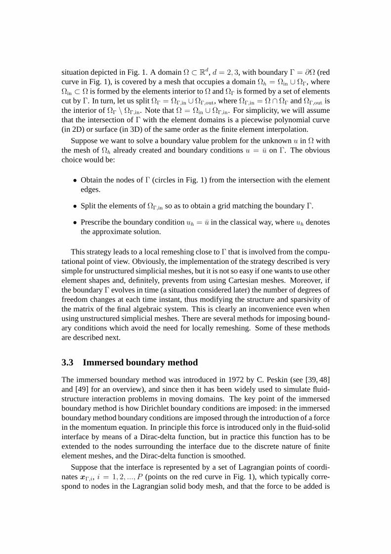
Before starting to describe the various methods, let us state which is the key issuewhen dealing with moving subdomains in fixed mesh strategies. Let us consider thesituation depicted in Fig. 2 attn, where we have a circular solid body immersed ina fluid which we want to simulate using a fixed mesh strategy. Wehave depicted ingreen nodes inside the fluid computational domain. Let us nowconsider the situationat time steptn+1, where the circular body has been horizontally displaced. Thereare nodes which were outside the flow computational domain attn, which are insidethe computational domain attn+1 (green nodes inside the red circle in Fig. 2). Thesenodes are callednewly created nodes. Since the unknown values at these nodes attn isnot known, computing temporal derivatives is not immediate. The following sectionsdescribe some of the proposed strategies to do so.

−1 0 1 2 3 4 5−1

−0.5

0

0.5

1

−1 0 1 2 3 4 5−1

−0.5

0

0.5

1

Figure 2: Green: nodes and elements inside the computational domain. Left: domainconfiguration attn. Right: domain configuration attn+1. The red circle correspondsto the domain configuration attn.

4.1 The fictitious domain method

In the fictitious domain method [22,24] we work with a computational domain whichdoes not coincide with the physical flow domain. Instead, we use as computationaldomain for the flow problem the whole region covered by the finite element mesh, thatis, we solve in both the green and black regions in Fig. 2. Obviously, we are not inter-ested in the solution inside the solid body region, which is physically meaningless.

The key point of the fictitious domain method is that, since wesolve for the wholecomputational domain, we can use the results attn for computing temporal derivativesat tn+1 even for the newly created nodes. Let us say, however, that results attn fornewly created nodes attn+1 do not come from a physical problem but from afictitiousone, and that it is not clear how results in both the physical and the fictitious problemare related.

The fictitious domain method has been extensively used to simulate two and three-dimensional flow problems with moving boundaries having a known trajectory, andin particular to the solution of a Couette problem and a helical ribbon mixer [7]. Asanother example, it has been applied to the solution of the flow around a movingdisk [25]. In fictitious domain methods, the motion of the object needs not necessarilyto be known a-priori, and aerodynamic forces can be taken into account to couple thefluid dynamics and the kinematics of the rigid body. Pan [46] predicts the path of aball falling in a viscous fluid (at low Reynolds numbers); in [20], the authors solve thetwo-dimensional flow around an airfoil that is free to rotatearound its center of mass,the sedimentation of particles in a box, and a three-dimensional case involving twospherical particles. Using the same method, Juarez [36] simulates the sedimentationof an elliptic body in a two-dimensional viscous fluid. This fictitious domain methodis also well-suited for shape optimization problems [21].

4.2 The fixed-mesh ALE method

The key point of the fixed-mesh ALE method is that, even if we are using a fixed-mesh method, domain movement cannot be obviated, and it is necessary to take itinto account with an ALE method. However, since we are interested in using a fixed-mesh, we develop a strategy which allows us to always work with the backgroundfixed mesh and, at the same time, includes the ALE terms which appear due to thedomain movement. We have developed this strategy in [2,14,15,32].

SupposeΩ0 is meshed with a finite element meshM0 and that at time leveltn

the domainΩ(tn) is meshed with a finite element meshMn (as we will see, close toM0). Let un be the velocity already computed onΩ(tn). The purpose is to obtainthe fluid regionΩ(tn+1) and the velocity fieldun+1. The former may move accordingto a prescribed kinematics, for example due to the motion of asolid, or can be anunknown of the problem. If the classical ALE method is used,Mn would deform toanother mesh defined attn+1. The key idea is not to use this mesh to computeun+1

andpn+1, but to re-mesh in such a way that the new mesh is, essentially, M0 onceagain.

The steps of the algorithm to achieve the goal described are the following:

1. DefineΓn+1

freeby updating the function that defines it.

2. Deformvirtually the meshMn to Mn+1

virt using the classical ALE concepts andcompute the mesh velocityun+1

m .

3. Write down the ALE Navier-Stokes equations onMn+1virt .

4. Split the elementsof M0 cut byΓn+1

freeto define a mesh onΩ(tn+1), Mn+1.

5. Projectthe ALE Navier-Stokes equations fromMn+1

virt to Mn+1.

6. Solve the equations onMn+1 to computeun+1 andpn+1.

A global idea of the meshes involved in the process is represented in Fig. 3. Notein particular that at each time steps two sets of nodes have tobe appropriately dealtwith, namely, the so called newly created nodes and the boundary nodes. Contraryto other fixed grid methods, newly created nodes are treated in a completely naturalway using the FM-ALE approach: the value of the velocity there is directly given bythe projection step fromMn+1

virt to Mn+1. Boundary nodes require either additionalunknowns with respect to those of meshM0 or an appropriate imposition of boundaryconditions, as explained in the previous Section.

4.3 Chimera strategies

The Chimera method was first envisaged as a tool for simplifying the mesh generation[5, 51, 52]. Independent meshes are generated for each component (object) of the

Figure 3: Two dimensional FM-ALE schematic. Top-left: original finite elementmeshM0 of Ω0. Top-right: finite element meshMn of Ω(tn), with the elementsrepresented by a thick line and the elements ofM0 represented by thin line. Theblue line representsΓn

free and the red edges indicate the splitting ofM0 to obtainMn.Bottom-left: updating ofMn to Mn+1

virtusing the classical ALE strategy. The position

of Γn+1

freeis again shown using a solid blue line and the previous positionΓn

free using adotted blue line. Bottom-right: MeshMn+1 of Ω(tn+1), represented by a thick line.The edges that split elements ofM0 are again indicated in red. Boundary nodes, whereapproximate boundary conditions need to be imposed, are drawn in green, whereasnewly created nodes are drawn in gray.

computational domain, enabling a flexibility on the choice of the type of element aswell as on their orientation that could not be possible when meshing complex threedimensional geometries [6,27]. Then, as a direct application, the Chimera method hasalso been used as a mesh refinement technique [47]. In addition, if it is implementedefficiently, it is a very efficient tool to treat flows with moving components [9,50,55].

Through the simple example sketched in Figure 4, let us briefly explain the Chimeramethod applied to the motion of moving objects inside a fluid domain:

• Independent meshes are generated for the so called background mesh and themesh around the solid, which is called thepatch mesh.

• The mesh around the solid is placed on the background mesh. The set of thetwo overset grids is the so calledcomposite grid. Elements of the backgroundlocated inside the patch are removed, with the possibility of having a non-emptyintersection between the resulting mesh and the patch mesh.This process,known ashole cutting, defines two interfaces, one of the domain attached tothe solid and the other, known asapparent interface, of the hole created in thebackground mesh. Nodes on this last interface are calledfringe nodes. Nodesbetween the apparent interface and the outer boundary of thepatch mesh are theoverlapping nodes.

• The problem defined on the patch mesh is again a fluid-structure interactionproblem. The main idea is to write the conservation equations on this domain ina frame of reference that moves with the rigid body motion of the solid. Then,the mesh deformation in the fluid region will be small, even ifthe solid deforms.Of course, the patch mesh will remain constant if the solid isa rigid body. Inorder to write the momentum conservation equation in the frame of referencefollowing the rigid body modes of the body, Coriolis, centrifugal forces andacceleration forces have to be added to the Navier-Stokes equations. These areof the form

2ρ ω × u, ρ ω × (ω × x) and − ρ as,

respectively, whereω is the angular velocity of the frame reference,x the posi-tion vector andas the acceleration.

• The FSI problem on the patch mesh is then coupled to the flow problem onthe background mesh using adomain decomposition strategy. Typically, aDirichlet-Dirichlet coupling is used (this is the so calledSchwartz’s method).This however requires a wide enough overlap to allow the associated iteration-by-subdomain strategy converge. Nevertheless, it is shownin [30, 31] that it isalso possible to apply a Dirichlet condition on the apparent(non-smooth) inter-face and a Neumann condition on the outer boundary of the patch domain. Notethat variables on the patch mesh and the background mesh willbe referred todifferent reference systems, and thus the former need to be properly transformedto the fixed reference where they are usually required.

Figure 4: Chimera method: principles.

The reader can see the details of this approach in [30], whereseveral examplessolved using this method can be found.

4.4 Other possibilities

As we have already seen, a special treatment is required for newly created nodes. Inmany publications, the previous time step values are computed using ad hoc argu-ments, that sometimes lead to good approximations from the practical point of viewwhen small time steps are used. As an example, in [43] the authors extrapolate thevelocity and pressure from the nearest fluid nodes at the previous time step. In [10],the Navier-Stokes equations are correctly expressed in an ALE framework, but thevelocity is taken as the solid velocity. It is worth to note that if the solid is deformableand has been solved together with the fluid in a coupled way (asin the original im-mersed boundary method [48] or in the fluid-solid approach in[58]), this velocity isphysically meaningful. This is not the case, however, in thecase of rigid bodies orbodies with rigid boundaries. A possibility to deal with this situation is to write theNavier-Stokes equations in a non-inertial frame of reference attached to the body, asin [38], where an immersed boundary method is used.

5 Summary

The purpose of this chapter has been to review some methods that allow to use fixedmeshes in problems with time dependent domains, with particular emphasis on thosein which the authors have been involved. The connection withthe approximate impo-sition of boundary conditions has been highlighted.

Summarizing, the methods described herein are:

• Approximate imposition of Dirichlet boundary conditions:

– Introduction of forces on the boundaries.

– Penalization of the boundary conditions, including Nitsche’s method.

– Use of Lagrange multipliers to enforce boundary conditions.

– Use of inactive degrees of freedom to optimize the imposition of boundaryconditions.

• Treatment of time dependent domains:

– Solving in the whole physical domain, both the solid and the fluid, withan appropriate modeling of the forces at the interface. Thisincludes theoriginal version of the immersed boundary method.

– Fictitious domain method, in which the solid is considered to be filled witha fictitious fluid and boundary conditions are imposed through Lagrangemultipliers.

– Fixed-mesh ALE method, based on the classical ALE approach but pro-jecting the equations always to a fixed mesh.

– Chimera strategies based on domain decomposition method, which at leastallow to remove the mesh deformation due to rigid body motions of thesolids inside the fluid.

Many variants of all these methods exist. Our purpose here has been to describethe main ideas behind them, without entering the details that can be found in thereferences.

References

[1] D.N. Arnold. An interior penalty finite element method with discontinuous ele-ments.SIAM Journal on Numerical Analysis, 19:742–760, 1982.

[2] J. Baiges and R. Codina. The fixed-mesh ale approach applied to solid mechanicsand fluid-structure interaction problems.International Journal for NumericalMethods in Engineering, 81:1529–1557, 2010.

[3] H.J.C Barbosa and T.J.R Hughes. The finite element methodwith Lagrangianmultipliers on the boundary: circumventing the Babuska-Brezzi condition.Com-puter Methods in Applied Mechanics and Engineering, 85:109–128, 1991.

[4] R. Becker, P. Hansbo, and R. Stenberg. A finite element method for domain de-composition with non-matching grids.Mathematical Modelling and NumericalAnalysis, 37:209–225, 2003.

[5] J.A. Benek, P.G. Buning, and J.L. Steger. A 3-D Chimera grid embedding tech-nique. In7th AIAA Computational Fluid Dynamics Conference, pages 322–331,Cincinnati (USA), July 15-17 1985. AIAA-1985-1523.

[6] J.A. Benek, T.L. Tonegan, and N.E. Suhs. Extended Chimera grid embeddingsystem with application to viscous flow. In8th AIAA Computational Fluid Dy-namics Conference, pages 283–291, June 9-11 1987. AIAA-87-1126.

[7] F. Bertrand, P.A. Tanguy, and F. Thibault. A three-dimensional fictitious do-main method for incompressible fluid flow problems.Int. J. Num. Meth. Fluids,25:719–736, 1997.

[8] E. Burman, M.A. Fernandez, and P. Hansbo. Continuous interior penalty finiteelement method for Oseen’s equations.SIAM Journal on Numerical Analysis,44:1248–1274, 2006.

[9] J.-J. Chattot and Y. Wang. Improved treatment of interstecting bodies with theChimera method and validation with a simple and fast flow solver. Computers &Fluids, 27(5-6):721–740, 1998.

[10] Y. Cheny and O. Botella. The LS-STAG method: A new immersed boundary /level-set method for the computation of incompressible viscous flows in complexmoving geometries with good conservation properties.Journal of ComputationalPhysics, 2008. Submitted.

[11] R. Codina. A stabilized finite element method for generalized stationary in-compressible flows.Computer Methods in Applied Mechanics and Engineering,190:2681–2706, 2001.

[12] R. Codina and J. Baiges. Approximate imposition of boundary conditions inimmersed boundary methods.Ijnme, 80:1379–1405, 2009.

[13] R. Codina and G. Houzeaux. Implementation aspects of coupled problems inCFD involving time dependent domains, inVerification and Validation Methodsfor Challenging Multiphysics Problems, G. Bugeda, J.C Courty, A. Guilliot, R.Hold, M. Marini, T. Nguyen, K. Papailiou, J. Periaux and D.Schwamborn (Eds.),pages 99–123. CIMNE, Barcelona, 2006.

[14] R. Codina, J. Houzeaux, H. Coppola-Owen, and J. Baiges.The fixed-mesh ALEapproach for the numerical approximation of flows in moving domains.Journalof Computational Physics, 228:1591–1611, 2009.

[15] H. Coppola-Owen and R. Codina. A finite element model forfree surfaceflows on fixed meshes.International Journal for Numerical Methods in Fluids,54:1151–1171, 2007.

[16] J. Donea, P. Fasoli-Stella, and S. Giuliani. Lagrangian and eulerian finite elementtechniques for transient fluid structure interaction problems. InTransactionsFourth SMIRT, page B1/2, 1977.

[17] A. Ern and J.-L. Guermond.Theory and Practice of Finite Elements. Springer-Verlag, 2004.

[18] L.P. Franca and S.L. Frey. Stabilized finite element methods: II. The incom-pressible Navier-Stokes equations.Computer Methods in Applied Mechanicsand Engineering, 99:209–233, 1992.

[19] A. Gilmanov and F. Sotiropoulos. A hybrid Cartesian/immersed boundarymethod for simulating flows with 3D, geometrically complex,moving bodies.Journal of Computational Physics, 207:457–492, 2005.

[20] R. Glowinski, T.-W. Pan, T.I. Hesla, D.D. Joseph, and J.Periaux. A distributedLagrange multiplier/fictitious domain method for flows around moving rigidbodies: application to particulate flow.Int. J. Num. Meth. Fluids, 30:1043–1066,1999.

[21] R. Glowinski, T.-W. Pan, J. Kearsley, and J. Periaux. Numerical simulation andoptimal shape for viscous flow by a fictitious domain method.Int. J. Num. Meth.Fluids, 20:685–711, 1995.

[22] R. Glowinski, T.-W. Pan, and J. Periaux. Fictitious domain methods for theDirichlet problem and its generlization to some flow problems. In K. Mor-gan, E. Onate, J. Periaux, J. Peraire, and O.C. Zienkiewicz, editors, Finite El-ement in Fluids, New Trends and Applications, pages 347–368. Pineridge Press,Barcelona (Spain), 1993.

[23] R. Glowinski, T.-W. Pan, and J. Periaux. A fictitious domain method for Dirich-let problems and applications.Computer Methods in Applied Mechanics andEngineering, 111:203–303, 1994.

[24] R. Glowinski, T.-W. Pan, and J. Periaux. A fictitious domain method for Dirich-let problems and applications.Computer Methods in Applied Mechanics andEngineering, 111:203–303, 1994.

[25] R. Glowinski, T.-W. Pan, and J. Periaux. On a domain embedding method forflow around moving rigid bodies. In Petter E. Bjørstad, MagneEspedal, andDavid Keyes, editors,Ninth international Conference of Domain DecompositionMethods. ddm.org, 1998. Proceedings from the Ninth International Conference,June 1996, Bergen, Norway.

[26] R. Glowinski, T.W. Pan, T.I. Hesla, D.D. Joseph, and J. Periaux. A distributedLagrange multiplier/fictitious domain method for flows around moving rigidbodies: application to particulate flow.International Journal for NumericalMethods in Fluids, 30:1043–1066, 1999.

[27] E. Guilmineau, J. Piquet, and P. Queutey. Two-dimensional turbulent viscousflow simulation past airfoils at fixed incidence.Computers & Fluids, 26(2):135–162, 1997.

[28] A. Hansbo and P. Hansbo. An unfitted finite element method, based on Nitsche’smethod, for elliptic interface problems.Computer Methods in Applied Mechan-ics and Engineering, 191:5537–5552, 2002.

[29] P. Hansbo and M.G. Larson. Discontinuous Galerkin methods for incompressibleand nearly incompressible elasticity by Nitsche’s method.Computer Methods inApplied Mechanics and Engineering, 191:1895–1908, 2002.

[30] G. Houzeaux and R. Codina. A Chimera method based on a Dirichlet/Neumann(Robin) coupling for the Navier-Stokes equations.Computer Methods in AppliedMechanics and Engineering, 192:3343–3377, 2003.

[31] G. Houzeaux and R. Codina. An overlapping iteration-by-subdomain Dirich-let/Robin domain decomposition method for advection–diffusion problems.Journal of Computational and Applied Mathematics, 158:243–276, 2003.

[32] G. Houzeaux and R. Codina. A finite element model for the simulation of lostfoam casting.International Journal for Numerical Methods in Fluids, 46:203–226, 2004.

[33] A. Huerta and W.K. Liu. Viscous flow with large free surface motion.ComputerMethods in Applied Mechanics and Engineering, 69:277–324, 1988.

[34] T.J.R. Hughes. Multiscale phenomena: Green’s function, the Dirichlet-to-Neumann formulation, subgrid scale models, bubbles and theorigins of stabi-lized formulations.Computer Methods in Applied Mechanics and Engineering,127:387–401, 1995.

[35] T.J.R. Hughes, W.K. Liu, and T.K. Zimmerman. Lagrangian-eulerian finite ele-ment formulation for incompressible viscous flows.Computer Methods in Ap-plied Mechanics and Engineering, 29:329–349, 1981.

[36] L.H. Juarez. Numerical simulation of the sedimentation of an elliptic body inan incompressible viscous fluid.C. R. Acad. Sci. Paris, 329(Serie IIb):221–224,2001.

[37] M. Juntunen and R. Stenberg. Nitsche’s method for general boundary conditions.Helsinki University of Technology, Institute of Mathematics, Research ReportsA530, 2007.

[38] D. Kima and H. Choi. Immersed boundary method for flow around an arbitrarilymoving body.Journal of Computational Physics, 212:662–680, 2006.

[39] M-C. Lai and C.S. Peskin. An immersed boundary method with formal second-order accuracy and reduced numerical viscosity.Journal of ComputationalPhysics, 160(2):705–719, 2000.

[40] Ming-Chih Lai and C.S. Peskin. An immersed boundary method with formalsecond-order accuracy and reduced numerical viscosity.Journal of Computa-tional Physics, 160:705–719, 2000.

[41] R.J. LeVeque and Z. Li. The immersed interface method for elliptic equationswith discontinuous coefficients and singular sources.SIAM Journal on Numeri-cal Analysis, 31 (4):1019–1044, 1994.

[42] R.J. LeVeque and Z. Li. Immersed interface method for incompressible Navier-Stokes equations.SIAM Journal on Scientific and Statistical Computing, 18(3):709–735, 1997.

[43] R. Lohner, J.R. Cebral, F.F. Camelli, J.D. Baum, and E.L. Mestreau. Adaptiveembedded/immersed unstructured grid techniques.Archives of ComputationalMethods in Engineering, 14:279–301, 2007.

[44] S. Marella, S. Krishnan, H. Liu, and H.S. Udaykumar. Sharp interface carte-sian grid method i: An easily implemented technique for 3d moving boundarycomputations.Journal of Computational Physics, 210:1–31, 2005.

[45] J. Mohd-Yusof. Combined immersed boundaries/B-splines methods for simu-lations of flows in complex geometries.CTR annual research briefs, StanfordUniversity, NASA Ames, 1997.

[46] T.-W. Pan. Numerical simulation of the motion of a ball falling in an incom-pressible viscous fluid.C. R. Acad. Sci. Paris, 327(Serie IIb):1035–1038, 1999.

[47] E. Part-Enander.Overlapping Grids and Applications in Gas Dynamics. PhDthesis, Uppsala Universitet, Sweden, 1995.

[48] C.S. Peskin. Flow patterns around heart valves: A numerical method.Journalof Computational Physics, 10:252–271, 1972.

[49] C.S Peskin. The immersed boundary method.Acta Numerica, pages 479–517,2002.

[50] N.C. Prewitt, D.M. Belk, and W. Shyy. Parallel computing of overset grids foraerodynamic problems with moving objects.J. Progr. Aero. Sci., 36:117–172,2000.

[51] J.L. Steger and J.A. Benek. On the use of composite grid schemes in computa-tional aerodynamics.Computer Methods in Applied Mechanics and Engineering,64:301–320, 1987.

[52] J.L. Steger, F.C. Dougherty, and J.A. Benek. A Chimera grid scheme. In K. N.Ghia and U. Ghia, editors,Advances in Grid Generation, volume ASME FED-5,pages 59–69, 1983.

[53] J.V. Voorde, J. Vierendeels, and E. Dick. Flow simulations in rotary volumetricpumps and compressors with the fictitious domain method.Journal of Compu-tational and Applied Mathematics, 168:491–499, 2004.

[54] X. Wang and WKLiu. Extended immersed boundary method using fem andrkpm. Computer Methods in Applied Mechanics and Engineering, 193:1305–1321, 2004.

[55] Z.J. Wang and V. Parthasarathy. A fully automated Chimera methodology formultiple moving body problems.Int. J. Num. Meth. Fluids, 33:919–938, 2000.

[56] S. Xu and Z.J. Wang. An immersed interface method for simulating the inter-action of a fluid with moving boundaries.Journal of Computational Physics,216:454–493, 2006.

[57] J.H. Ferziger Y.H. Tseng. A ghost-cell immersed boundary method for flow incomplex geometry.Journal of Computational Physics, 192:593–623, 2003.

[58] H. Zhao, J.B. Freund, and R.D. Moser. A fixed-mesh methodfor incompressibleflow-structure systems with finite solid deformations.Journal of ComputationalPhysics, 227:3114–3140, 2008.