Bachelorarbeit Fakult¨ at f¨ ur Mathematik und Informatik Lehrgebiet Analysis SS2021 Fixed Point Theorems for Real- and Set-Valued Functions in Finite- and Infinite-Dimensional Spaces Fabian Smetak Studiengang: B.Sc. Mathematik Matrikelnummer: 7783680 FernUniversit¨ at in Hagen Betreuer: Prof. Dr. Delio Mugnolo Dr. Matthias T¨aufer Mai 2021
Transcript
Bachelorarbeit
Fakultat fur Mathematik und Informatik
Lehrgebiet Analysis
SS2021
Fixed Point Theorems for Real- and
Set-Valued Functions in Finite- and
Infinite-Dimensional Spaces
Fabian Smetak
Studiengang: B.Sc. Mathematik
Matrikelnummer: 7783680
FernUniversitat in Hagen
Betreuer: Prof. Dr. Delio Mugnolo
Dr. Matthias Taufer
Mai 2021
Abstract
Fixed point theorems play an important role in various branches of mathematics
and have diverse applications to other fields. At its core, this thesis is devoted to
the fixed point theorem of Brouwer which states that a continuous function on a
nonempty, compact and convex subset of a finite-dimensional space must have a
fixed point. Although the theorem can be proven analytically, this thesis follows a
different approach: We use Sperner’s lemma – an important result from combina-
torial topology – and simplicial subdivisions to show that any continuous function
mapping a simplex into itself must have a fixed point. We then extend the theo-
rem to sets that are homeomorphic to simplices. The second part of the thesis is
concerned with generalizations of Brouwer’s fixed point theorem. On the one hand,
the restriction to finite-dimensional spaces is relaxed. By introducing the concept of
compact operators, Schauder’s fixed point theorem is established – an analogue to
Brouwer’s theorem for infinite-dimensional spaces. On the other hand, the concept
of point-to-point mappings (i.e. functions) is generalized and point-to-set mappings
(so-called correspondences or set-valued functions) are introduced. These consider-
ations lead to Kakutani’s fixed point theorem, a result that has gained significant
traction in applications such as economics or game theory. This is illustrated by
using Kakutani’s fixed point theorem to establish existence of pure-strategy Nash
equilibria in a certain class of games. The first and foremost objective of this thesis
is to provide an accessible and intuitive introduction to fixed point theorems and to
pave the way for more advanced studies in this subject area.
B.3 Homeomorphism between a simplex and a closed ball . . . . . . . . . . . . 73
References 75
Declaration of Authorship 77
I
Acknowledgments
I would like to express my sincere gratitude to Prof. Dr. Delio Mugnolo and Dr. Matthias
Taufer who served as the supervisors of this thesis. They were the ones who introduced
me to the study of fixed point theorems in a seminar at the University of Hagen. The
experiences I was able to gain there had a significant impact on the writing of this thesis.
In fact, Dr. Taufer pointed out to me that the proof of Brouwer’s fixed point theorem
can be approached by means of Sperner’s lemma in the first place. Prof. Dr. Mugnolo
laid the foundation of basically all of my understanding of topics in real- and functional
analysis by means of his excellent teaching of and support with the analytical courses at
the Universtiy of Hagen. Moreover, I am very thankful for the approachability of Prof.
Dr. Mugnolo and Dr. Taufer who always responded immediately to any inquires I had
during the course of this thesis. Finally, I was very lucky to have been given a tremendous
amount of freedom in the topic selection and in the general approach I took in this thesis.
This enabled me to explore topics that go well beyond Brouwer’s fixed point theorem and
to shape my understanding of many interesting concepts in the subject area of analysis.
1
List of Figures
Figure 1 Brief overview of the main steps of this thesis. page 4
Figure 2 Examples and counterexamples of convex sets. page 6
Figure 3 Different N-simplices. page 7
Figure 4 Examples and counterexamples of simplicial subdivisions. page 9
Figure 5 Different simplicial subdivisions. page 9
Figure 6 The Sperner labeling condition. page 11
Figure 7 Proof idea of Brouwer’s fixed point theorem. page 15
Figure 8 Barycenter for different N-simplices. page 17
Figure 9 Barycentric subdivisions of different orders. page 18
Figure 10 The helper function k to construct homeomorphisms. page 22
Figure 11 Homeomorphism between simplex and closed ball. page 27
Figure 12 Sufficient conditions of Brouwer’s FPT. page 31
Figure 13 Brouwer’s FPT and the number of fixed points. page 32
Figure 14 Key steps to generalize Brouwer’s fixed point theorem. page 33
Figure 15 Illustration of a correspondence. page 48
Figure 16 Example and counterexample for upper semi-continuity. page 49
Figure 17 Sufficient conditions of Kakutani’s FPT. page 56
Figure 18 Kakutani’s FPT and the number of fixed points. page 57
Figure 19 Analytical proof idea of Brouwer’s fixed point theorem. page 66
Figure 20 Proof idea – Homeomorphism: simplex and closed ball. page 73
2
1 Introduction
The study of fixed point theorems has not only become an integral part of many branches
in mathematics but has gained significant traction in applications to other quantitative
disciplines. One of the best-known and most fundamental results is the fixed point theorem
of Banach according to which strictly contractive self-mappings on complete metric spaces
must have a unique fixed point. On the one hand, this result is appealing since it does
not only guarantee uniqueness of the fixed point but also provides a constructive method
of how to find it. On the other hand, the required assumptions on the mapping are strong
and could be difficult to verify. Another well-known result, Brouwer’s fixed point theorem,
is of a somewhat different nature: While its prerequisites on the self-mapping are relatively
weak, it requires stronger assumptions on the underlying sets and spaces. More precisely,
it states that any continuous function mapping a nonempty, compact and convex set into
itself must have at least one fixed point. At its core, this thesis is devoted to the study
of Brouwer’s theorem. Instead of a pure analytical approach, we1 use Sperner’s lemma
and simplicial subdivisions to offer a proof of Brouwer’s fixed point theorem that is very
accessible and only requires elementary tools from convex analysis. The aim of this thesis
is twofold and some important notes should be made in this context:
1. My first and foremost objective is to provide an inherently accessible and intuitive
approach to an important class of fixed point theorems. I have tried to aggregate
insights from many different authors and sources and to present all concepts and
proofs in a very detailed manner. On the one hand, this conflicts in a sense with the
mathematical spirit of parsimony and conciseness. On the other hand, the thesis is
self-contained and does not require repetitive references to result from other sources.
2. My second goal is to go beyond the fixed point theorem of Brouwer and to look at
two important generalizations that derive from it: Schauder’s fixed point theorem
for infinite-dimensional spaces and Kakutani’s fixed point theorem for set-valued
functions.
Moreover, I have tried to offer many graphical illustrations in order to visualize important
concepts and to provide additional perspectives to some of the results. The rest of this
thesis proceeds as follows. Section 2 revises fundamental concepts from convex analysis
and introduces Sperner’s lemma. Section 3 constitutes the main part of this thesis. It
1Although this is a single-authored thesis, I will often follow the common convention and use ”we” insteadof ”I”. In my personal opinion, this is phonetically more appealing but can also be understood as ”wethe readers” as I am myself not an expert but rather a keen learner of the subject matter.
3
states and proves Brouwer’s fixed point theorem for simplices and for sets that are home-
omorphic to them. Section 4 deals with Schauder’s fixed point theorem which generalizes
the result of Brouwer to infinite-dimensional spaces. Section 5 offers a generalization to
set-valued functions and introduces Kakutani’s fixed point theorem while section 6 con-
cludes. Appendix A illustrates the idea of an analytical proof of Brouwer’s fixed point
theorem while appendix B collects proofs of some auxiliary results. The following figure
summarizes the pursued path of this thesis.
Figure 1: Brief overview of the main steps of this thesis.
4
2 Sperner’s Lemma and Simplices
The core of this thesis is devoted to Brouwer’s fixed point theorem, not least because many
other fixed point results derive from it or constitute mere generalizations to other settings.
Although the theorem can be proven in an analytical way, the proof is lengthy and re-
quires a relatively sophisticated machinery of tools, some of which include topological
no-retraction theorems and Gauss’s divergence theorem.2 By contrast, Sperner’s lemma -
an important result in combinatorial topology (Sperner, 1928) - allows to prove Brouwer’s
fixed point theorem by means of only elementary tools. There exist various (compara-
ble) ways to prove Sperner’s Lemma - some authors use a graph-theoretic approach (e.g.
Border, 1985; Yuan, 2017) while others draw from tools that are more of combinatorial
nature (e.g. Meister, 2018). Both approaches inherently rely on simplices and simplicial
subdivisions among others. The following paragraph gathers important concepts that are
needed to formulate and then to prove Sperner’s lemma.
2.1 Fundamental definitions and terminology
Most of the required terminology describes basic concepts from convex analysis, the most
fundamental of which is that of a convex set.
Definition 2.1 (Convex set) [LL15; AY17]
A subset A ⊂ Rn is convex if and only if whenever x and y are two points from A, then
the entire segment [x, y] is a subset of A. Equivalently, A is convex if for all x, y ∈ A and
λ ∈ [0, 1] ⊂ R, we have λx+ (1− λ)y ∈ A.
Intuitively, a convex set cannot contain any holes or bumps since the entire (line) segment
connecting two points of the set must again be contained in it. For our purposes, Rn and
any linear subspaces of Rn will constitute important convex sets.
Another important concept towards defining simplices is that of a convex hull. For a set
A ⊂ Rn, the convex hull of A is defined as the intersection of all convex subsets K ⊂ Rn
with A ⊂ K which is nothing but the smallest convex set that contains A (Zeidler, 1995).
For our purposes, however, we will readily define convex hulls by means of finite convex
combinations.
2I have presented an analytical proof of Brouwer’s fixed point theorem in a seminar at the Universityof Hagen. Appendix A summarizes some of the fundamental steps in a figure. Detailed materials areavailable upon request.
5
Figure 2: Examples (left) and counterexamples (right) of convex sets (Source: LL15).
Definition 2.2 (Convex combination) [LL15; AY17]
Let x1, ..., xN ∈ Rn and let λ1, ..., λN ∈ R. We call the linear combination
N∑i=1
λixi = λ1x
1 + λ2x2 + · · ·+ λkx
N
convex combination if λi ≥ 0 for 1 ≤ i ≤ N and∑N
i=1 λi = 1.
Definition 2.3 (Convex hull) [KB85]
For A ⊂ Rn, the convex hull of A, denoted by co(A), is the set of all finite convex
combinations of points in A, i.e.
co(A) ={ N∑i=1
λixi∣∣ xi ∈ A, λi ≥ 0 for 1 ≤ i ≤ N,
N∑i=1
λi = 1}.
A final notion that is required to define simplices is that of affine independence.
Definition 2.4 (Affine independence) [KB85; EZ95]
Let λ0, ..., λN ∈ R. The set {x0, ..., xN} ⊂ Rn is affine independent if∑N
i=0 λixi = 0
and∑N
i=0 λi = 0 imply λ0 = λ1 = ... = λN = 0.
Affine independence can be equivalently defined as {x1 − x0, ..., xN − x0} to be linearly
independent and this definition does not depend on the numbering of the points. Some
authors also call an affine independent set to be in general position (Toenniessen, 2017;
Rotman, 1988). Three points in R2 are affine independent if they form a triangle and
hence do not lie on a straight line. We are now in a position to define the fundamental
concept of N -simplices. Many authors follow Kuratowski (1972) and make simplices open
sets (Border, 1985; Yuan, 2017); we will directly define simplices as to be closed sets.
6
Definition 2.5 (N-simplex and vertices ) [KJ08; EZ95]
Let N ∈ N. An N-simplex S (or N-dimensional simplex) in Rn is the convex hull of an
affine independent set of N+1 points x0, ..., xN ∈ Rn. Formally,
S := co({x0, ..., xN}) ={ N∑i=0
λixi∣∣ xi ∈ Rn, λi ≥ 0 for 0 ≤ i ≤ N,
N∑i=0
λi = 1}.
The points x0, ..., xN are called vertices of the simplex S.
Figure 3 below illustrates N-simplices for N ∈ {0, 1, 2, 3}. 2-simplices (i.e. triangles) will
become particularly important as they provide an excellent starting point to graphically
illustrate most of the concepts discussed in the following.
Figure 3: Different N-simplices (Source: KJ08; MB20).
Simplices can be regarded as a special case of convex hulls that require the points x0, ..., xN ∈Rn to be affine independent. The so-called standard n-simplex is of particular interest in
some of the subsequent proofs.
Definition 2.6 (Standard n-simplex in Rn+1) [KB85; HM18]
The standard n-simplex ∆n is the subset of Rn+1 that is spanned by the (n+1) basis
vectors e1, ..., en+1 ∈ Rn+1, i.e. by the vertices
There is a canonical map from the standard n-simplex to any arbitrary n-simplex with
vertices (v0, ..., vn) given by (x0, ..., xn) ∈ ∆n 7→∑n
i=0 xivi ∈ co({v0, ..., vn}).
We will be particularly interested in working with vertices, edges, and other ”sides” of
simplices. The following definition provides the necessary ground to do so.
Definition 2.7 (Face, k-face and boundary of a simplex) [KJ08; JR88; EZ95]
Let S be an N-Simplex with vertices x0, ..., xN ∈ Rn. A face of S is the convex hull of
a (not necessarily proper) subset of {x0, ..., xN}. The k-face of S is the convex hull of
k + 1 distinct vertices of S where k = 0, 1, ..., N . A k-face of a simplex is also called a
k-dimensional subsimplex. The boundary ∂S of S is the union of its (N-1)-faces.
Figure 3(d) exemplifies a 0-face (red point), a 1-face or edge (blue line) and a 2-face (gray
area) using a 3-simplex.3 The following definition is fundamental for the rest of this section
and in particular for Sperner’s lemma and the proof of Brouwer’s fixed point theorem in
the next section. It describes a distinct way of how N-simplices can be ”subdivided” into
smaller N-subsimplices.
Definition 2.8 (Simplicial subdivision and mesh) [KB85; ES28; EZ95]
Let S := co({x0, ..., xN}) be an N-simplex where N ≥ 1. A simplicial subdivision (or
triangulation) of S is a finite collection S1,S2, ...,SJ , J ∈ N, of N-subsimplices satisfying
the following two conditions.
1.) S =J⋃j=1
Sj
2.) For any j, k ∈ {1, ..., J} with j 6= k, the intersection Sj ∩ Sk is either empty or equal
to a common face.
The mesh of a simplicial subdivision is the diameter of the largest subsimplex where the
diameter δ(S) of a simplex S := co({x0, ..., xN}) is defined by
δ(S) := supj,k∈{0,...,N}
‖xj − xk‖
and is hence equal to the largest of its 1-faces.4
3In general, a k-simplex has k+1Cs+1 :=(k+1s+1
)s-dimensional faces (Nikaido, 1968). In the above example,
the 3-simplex therefore has 4C3 :=(43
):= 4!
3!(4−3)! = 4 2-faces which can be seen in Figure 3(d).4Unless otherwise stated, we will use the Euclidean norm ‖·‖2 for the remainder of this text.
8
Figure 4 below illustrates the concept of a simplicial subdivision for the case of a triangle
(2-simplex). There are two particularly important examples of simplicial subdivisions:
equilateral subdivisions and barycentric subdivisions, both of which can be used in proving
Brouwer’s fixed point theorem by means of Sperner’s lemma.5 Figure 5 uses a 2-simplex
to illustrate different simplicial subdivisions.
Figure 4: The left picture does not constitute a simplicial subdivison as it violates condi-tion 2). The right picture shows a simplicial subdivison of a 2-simplex (Source: AY17).
Figure 5: Different simplicial subdivisions of a 2-simplex (Source: MB20).
Given a simplicial subdivision of a simplex S, we denote by V the set of all vertices of
all subsimplices of the subdivision.6 Sperner’s lemma makes a statement about so-called
Sperner simplices for simplicial subdivisions where V is labeled in a specific way.
5In fact, the proof only requires some simplicial subdivision with (arbitrarily) small mesh. By choosingthe divisions fine enough, both equilateral and barycentric subdivisions fulfill this property (see section3.1 for corresponding details on the barycentric subdivision and appendix B.1 for a detailed proof).
6This includes the vertices of the original simplex, vertices of subsimplices located on the boundary of theoriginal simplex as well as vertices of subsimplices that are in the interior of the original simplex.
9
Definition 2.9 (Carrier) [KB85; AY17]
Let P(A) denote the power set of a set A and let y be contained in the convex hull of the
vectors x0, ..., xN ∈ A, i.e. y =∑N
i=0 λixi with λi ≥ 0 for i ∈ {0, ..., N} and
∑Ni=0 λi = 1.
We define the set-valued function χ : co(A) → P({0, ..., N}) by χ(y) = {i | λi > 0}.It follows that if χ(y) = {i0, ..., ik}, then y ∈ co({xi0 , ..., xik}) and we call this face the
carrier of y.
Definition 2.10 (Proper labeling and Sperner simplices) [KB85; HM18; AY17]
Let V denote the vertices of all subsimplices of a simplicial subdivision of an N-simplex
S := co({x0, ..., xN}). Each function f : V → {0, ..., N} is called a labeling function. We
call f a proper labeling of the subdivision if f(v) ∈ χ(v) for all v ∈ V . An N-simplex is
called completely labeled or a Sperner simplex if f takes on all values 0, ..., N on its
vertices.
Intuitively, a proper labeling function can only assign the ”index values” to a vertex of
a subsimplex of those vertices of the original simplex that were needed to ”span” this
given vertex of the subsimplex by a convex combination. To facilitate intuition further,
we could equivalently define a proper labeling by the following condition which I will call
Let S1, ...,SJ , J ∈ N, be a simplicial subdivision of the N-simplex S. We say that the
labeling function f : V → {0, ..., N} complies with the Sperner labeling condition if
each vertex of Sj, j ∈ {1, ..., J}, is assigned a value 0, 1, ..., N such that the following
condition holds: If
v ∈ co({xi0 , ..., xik}), k = 1, ..., N, (2.1)
then one of the numbers i0, ..., ik is associated with v, i.e. f(v) ∈ {i0, ..., ik}.
Note that condition (2.1) in particular implies that each vertex xj, j ∈ {0, ..., N}, of
the original N-simplex S carries the number j since xj ∈ co({xj}).8 Figure 6 below
illustrates the Sperner labeling condition for a 2-simplex and an equilateral subdivision.
For illustrative purposes, I follow Berger (2020) (and many other authors in the literature)
7Definitions 2.10 and 2.11 are not only equivalent but essentially the same. The latter merely concentratesexplicitly on the vertices of the subsimplices S1, ...,SJ while the former ”subsumes” all of those verticeswithin V .
8Also note that condition (2.1) uses double subscripts (i.e. co({xi0 , ..., xik}) instead of co({x0, ..., xk}).This is necessary since convex hulls do not have to be formed by the first k vertices.
10
and use colors instead of numbers as labels.9 Subfigures 6b.) and 6c.) show that vertices
on the edge of the original simplex (i.e. v ∈ co{x0, x1}, v ∈ co{x1, x2} and v ∈ co{x0, x2})can only be labeled with the colors of the lowest-dimensional faces of the original simplex
S that contain the given vertices of a subsimplex. Subfigure 6d.) labels all vertices in
the interior of the original simplex (i.e. all v ∈ co{x0, x1, x2}) and shows that these
points can be labeled arbitrarily by either red, blue, or orange since the Sperner labeling
condition does not impose any further restrictions. Subfigure 6d.) also highlights all
Sperner simplices of the simplicial subdivision (i.e. all subtriangles that are completely
labeled with all three different colors on their vertices). In this example, the simplicial
subdivision gives rise to a unique Sperner simplex. The question arises whether every
labeling of a simplicial subdivision that adheres to the Sperner labeling condition gives
rise to the existence of such Sperner simplices. Sperner’s lemma proves that this is indeed
the case.
Figure 6: Illustration of the Sperner labeling condition (Source: MB20).
9In Figure 6, red is used for 0, blue is used for 1, and orange is used for 2.
11
2.2 Sperner’s lemma
Sperner’s lemma establishes that the number of completely-labeled N-subsimplices (i.e.
Sperner simplices) for any properly-labeled simplicially-subdivided simplex is odd (Yuan,
2017). Since zero is an even number, existence of such simplices follows immediately.10
Let S1, ...,SJ , J ∈ N, be a simplicial subdivision of the N-simplex S that is properly labeled
by the function f (i.e. that fulfills the Sperner labeling condition (2.1)). Then the number
of completely labeled (Sperner) N-subsimplices Sj is odd. In particular, there exists at least
one such Sperner simplex.
Proof: By induction on N , the dimension of the simplex.
Step 1:
Base case: For N = 0, the 0-simplex S is a single point, i.e. S = co({x0}) = x0 and
there do not exist other possibilities of simplicial subdivisions.11 By the Sperner labeling
condition (2.1), it must hold that f(x0) = 0. There is thus only one completely labeled
subsimplex, x0 itself, and this is an odd number.
Step 2:
Although not strictly necessary, we look at N = 1 to provide some additional clarity.
Each 1-subsimplex Sj is a line segment. For the remainder, we will call a (N-1)-face of
Sj distinguished if and only if its vertices carry at least the numbers {0, ..., N − 1}. For
N = 1, this means that a 0-face (i.e. a vertex) of Sj is called distinguished if it is labeled
by the number 0. For any 1-subsimplex Sj, there are precisely two possibilities:
1. The line segment Sj has exactly one distinguished (N-1)-face (in which case it must
be completely labeled, i.e. a Sperner simplex).
2. Sj has either two (both vertices labeled 0) or no (both vertices labeled 1) distin-
guished (N-1)-faces (in which case it is not a Sperner simplex).
Precisely one vertex of S = co({x0, x1}) is labeled with 0 (namely x0) while the other is
labeled with 1 (namely x1). No matter how the interior points are labeled, one always has
10Although the basic idea of proving Sperner’s lemma is always very similar, the nuances by which it ispresented vary across different sources. I will focus on a proof that is more of combinatorial nature.By introducing elementary concepts from graph theory, the proof can be shortened and presented in aslightly different manner (see for instance Border, 1985; Yuan, 2017, among others).
11Some authors argue that for N = 0, there is no simplicial subdivision of a single point, but the singlepoint is obviously an odd number (e.g. Meister, 2018).
12
to change numbers (from 0 to 1 or from 1 to 0) an odd number of times to get from the
0-corner to the 1-corner.12 Thus, the number of Sperner simplices must be odd.
Step 3:
Induction hypothesis : Suppose the statement of Sperner’s lemma holds for a fixed (but
arbitrary) N − 1 ∈ N.
Step 4:
Induction step: We show that the statement also holds for N . To do so, we consider a
properly labeled simplicial subdivision S1, ...,SJ , J ∈ N, of the N-simplex S. Again, there
are two possibilities for any N -subsimplex Sj:
1. Sj has exactly one distinguished (N-1)-face (in which case it must be completely
labeled, i.e. a Sperner simplex).
2. Sj has either two (all labels {0, ..., N−1} appear at some of its vertices while exactly
one label k ∈ {0, ..., N − 1} appears twice) or no distinguished (N-1)-faces (in which
case it is not a Sperner simplex).
We introduce the following designations:13
→ e denotes the number of completely labeled simplices Sj (i.e. Sperner simplices).
Our goal is to show that e is an odd number.
→ f denotes the number of almost completely labeled simplices Sj, i.e. simplices whose
vertices are labeled with the numbers 0, 1, ..., N − 1 but not with N , i.e. f(Sj) =
{0, 1, ...N − 1}.
→ g denotes the number of distinguished (N-1)-faces of any Sj in the interior of S.
→ h denotes the number of distinguished (N-1)-faces of any Sj on the boundary of S.
We are now in a position to systematically count the total number of (N-1)-faces by
considering each Sj separately:
12To see this, it is easiest to consider what happens to the number of Sperner simplices once changes tointerior labels are made. Consider any three adjacent vertices of the simplicial subdivision. There arethree possible cases which we illustrate based on a vertex that is labeled with 0 initially and is changedto 1. Case 1: A 0-vertex surrounded by two other 0-vertices is changed to 1, i.e. 0-0-0 becomes 0-1-0.This increases the number of Sperner simplices by 2. Case 2: A 0-vertex surrounded by two 1-verticesis changed to 1, i.e. 1-0-1 becomes 1-1-1. This decreases the number of Sperner simplices by 2. Case3: A 0-vertex surrounded by one 0-vertex and one 1-vertex is changed to 1, i.e. 0-0-1 becomes 0-1-1.This merely changes the position of the Sperner simplex. In all cases, Sperner simplices are changedby an even number and since there must be at least one additional change from 0 to 1 from x0 to x1
somewhere, we must change numbers an odd number of times in total.13I adhere to the original notation used by Sperner (1928).
13
1. Each completely labeled subsimplex Sj has precisely one distinguished (N-1)-face (⇒1 · e). Each almost completely labeled subsimplex Sj has exactly two distinguished
(N-1)-faces (⇒ 2 · f).
2. By counting all subsimplices Sj in this way, we will count each distinguished (N-1)-
face which is located in the interior of S twice since each (N-1)-face of a simplicial
subdivision in the interior of S belongs to precisely two different Sj (⇒ 2 · g). By
contrast, all (N-1)-faces located on the boundary of S (and are hence a subset of
co({x0, x1, ..., xN−1})) are counted only once (⇒ 1 · h). This yields the following
equation:
e + 2 f = 2 g + h. (2.2)
3. Since the simplicial subdivision is properly labeled by f (i.e. fulfills the Sperner
labeling condition (2.1)), we know that distinguished (N-1)-faces on the boundary
of S can only appear on a single (N-1)-face of S - namely the one labeled with
{0, 1, ..., N − 1}.14 We are hence in the (N − 1)-dimensional case and know by our
induction hypothesis that the number of Sperner simplices in this case is odd. In
other words, h is odd. It follows immediately from equation (2.2) that e must also be
odd. But e is precisely the number of Sperner simplices in the N -dimensional case.
By induction, Sperner’s lemma holds for any N ∈ N which completes the proof.
�
2.3 Relation to fixed point theory
The remainder of this thesis focuses exclusively on fixed point theorems for real- and set-
valued functions. Given a set M and a mapping f : M → M , x ∈ M is called a fixed
point of f if f(x) = x. At first sight it does not seem obvious how the existence of Sperner
subsimplices in a properly labeled simplicial subdivision relates to fixed point theory at
all. The first and foremost connection lies in the structural property of simplices. As will
be shown in the subsequent chapter, simplices are homeomorphic to closed balls which
in turn are homeomorphic to nonempty, compact, convex subsets of Rn. The latter form
the building block of Brouwer’s fixed point theorem. Therefore, we can begin by proving
existence of fixed points of functions that map a given simplex into itself. By means of
simplicial subdivisions that allow for an arbitrarily small mesh, such fixed points can always
14This is because each vertex xj of S is labeled by j, so there can only exist one such (N-1)-face labeledby {0, 1, ..., N − 1}:
14
be found via Sperner simplices which must exist by Sperner’s lemma.15 The existence of
such fixed points can then be ”transferred” from simplices to homeomorphic sets which
eventually proves Brouwer’s fixed point theorem. Figure 7 illustrates the individual steps
while the subsequent chapter formalizes these ideas.
Figure 7: Illustration of the key steps to prove Brouwer’s fixed point theorem via Sperner’slemma and simplicial subdivisions.
15Both equilateral and barycentric subdivisions have the property of being simplicial subdivisions whosemesh can be made arbitrarily small. Since most authors are only interested in using Sperner’s lemmato prove fixed point theorems, they directly use these special subdivisions when formulating Sperner’slemma (e.g. Meister, 2018; Nikaido, 1968). Moreover, in all what follows, Sperner’s lemma is solelyneeded to establish existence of completely labeled subsimplices - the ’odd number property’ as such isnever used (although it was essential to establish existence which immediately results from this property).
15
3 Brouwer’s Fixed Point Theorem
One of the best-known fixed point theorems is doubtlessly the Banach fixed point the-
orem. It requires relatively few assumptions on the underlying space but fairly strong
assumptions on the respective mapping.16 Brouwer’s fixed point theorem, by contrast,
only requires the function to be continuous but puts stronger assumptions on the space
(Brouwer, 1912). Albeit different versions of the theorem exist, the most general one that
we are interested in is the following.
Theorem 3.1 (Brouwer’s fixed point theorem) [DW18]
Let C ⊂ Rn be a nonempty, compact and convex set and let f : C → C be continuous.
Then f has at least one fixed point, i.e. there exists ξ ∈ C with f(ξ) = ξ.
Chronologically, Sperner’s lemma has been proven years after Brouwer’s fixed point the-
orem (Brouwer, 1912; Sperner, 1928) but it can significantly simplify the proof of the
latter.17 The next paragraph provides some necessary notions and properties of a partic-
ular simplicial subdivision before the proof of the above version of Brouwer’s fixed point
theorem will be successively developed.
3.1 The barycentric subdivision
The proof of Brouwer’s fixed point theorem via Sperner’s lemma relies on a simplicial
subdivision whose mesh can be made (arbitrarily) small - the barycentric subdivision fulfills
this property. We collect some necessary definitions before this can be shown formally.
Definition 3.2 (Barycentric coordinates and barycenter) [ADQ12; FT17]
Let {x0, ..., xN} ⊂ Rn be affine independent and let x ∈ S = co({x0, ..., xN}) with
x =N∑j=0
λjxj and
N∑j=0
λj = 1, λ0, ..., λN ∈ R, λj ≥ 0 ∀j.
Then, the unique λ0, ..., λN are called the barycentric coordinates of x. The barycen-
ter of S is given by
b(S) :=1
N + 1
N∑j=0
xj.
16The space has to be a nonempty, complete metric space while the function has to be a strict contraction.The latter property could be particularly difficult to verify.
17See appendix A for an idea of how to prove Brouwer’s fixed point theorem using analytical tools thatdoes not rely on Sperner’s lemma or simplicial subdivisions.
16
All barycentric coordinates are identical at the barycenter (i.e. λ0 = ... = λN = 11+N
).
The latter can hence be thought of as the center of gravity of the simplex (Rotman, 1988).
Figure 8 illustrates this idea by means of different N-simplices.
Figure 8: Illustration of the barycenter for different N-simplices (Source: MB20).
The concept of the barycenter can be used to inductively define the barycentric subdivision.
Definition 3.3 (Barycentric subdivision) [JR88]
The barycentric subdivision Sd(S) of an N-simplex S is a family of N-subsimplices
defined inductively as follows:
(i) The barycentric subdivision of a 0-simplex is the 0-simplex itself.
(ii) If φ0, φ1, ..., φN are the (N-1)-faces of the N-simplex S and if b is the barycenter of
S, then Sd(S) consists of all N-subsimplices spanned by b and the (N-1)-subsimplices
of the barycentric subdivisions Sd(φi), i = 0, ..., N .
Intuitively, an N-simplex can be barycentrically subdivided into (N+1)! smaller subsim-
plices (Toenniessen, 2017). To subdivide a 2-simplex (i.e. a triangle) S = co({x0, x1, x2}),for instance, we start by subdividing 0- and 1-simplices first: The barycentric subdivisions
of the 0-simplices (x0, x1, x2) are the simplices themselves. The barycentric subdivision
of the faces (1-simplices) each consists of two 1-subsimplices (line segments from the re-
spective corners to the barycenters b0, b1, b2). Finally, the barycentric subdivision of the
triangle is obtained by combining its barycenter b with the barycenters b0, b1, b2 of the 1-
simplices and the barycenters x0, x1, x2 of the 0-simplices. The result is the so-called first
barycentric subdivision of the 2-simplex and is illustrated in figure 9a) below. Barycen-
trially subdividing the N-subsimplices of the barycentric subdivision again leads to the
second barycentric subdivision (see figure 9b)). This process can be iterated which results
in successively finer (in terms of the mesh) simplicial subdivisions of the original simplex.
This observation is a key ingredient for the proof of Brouwer’s fixed point theorem and is
17
stated formally in the following proposition.18 It suggests that the mesh can be made ar-
bitrarily small by repeated barycentric subdivision. We call smaller N-subsimplices which
result from a k-times application of the barycentric subdivision of S derived subsimplices
of order k.
Proposition 3.4 (Mesh and iterated barycentric subdivision) [ADQ12; HN68]
Let S = co({x0, x1, ..., xN}) be an N-simplex with diameter δ(S) = supj,k∈{0,...,N}‖xj − xk‖and let Sk be any derived simplex of order k in the kth barycentric subdivision of S. Then
the following inequality holds:
δ(Sk) ≤( N
N + 1
)kδ(S). (3.1)
In particular, limk→∞
δ(Sk) = 0.
Proof: By induction on N , the dimension of the N-simplex.
→ See appendix B.1.
Figure 9: First four barycentric subdivisions of a 2-simplex(Source: https://en.wikipedia.org/wiki/Barycentric_subdivision).
3.2 Brouwer’s fixed point theorem for simplices
We are now in a position to develop the proof of Brouwer’s fixed point theorem by means
of barycentric subdivisions and Sperner’s lemma. We will follow the individual steps as
illustrated in figure 7 and begin by proving a fixed point theorem for N-simplices.
18Although the proof for this result can be found in some textbooks on algebraic topology, surprisinglyfew sources provide the proof in the context of Brouwer’s fixed point theorem but simply take it asgiven.
Proposition 3.5 (Brouwer’s fixed point theorem for N-simplices) [MB20; HM18]
Let S = co({x0, ..., xN}) denote an N-simplex. Any continuous map f : S → S has at least
one fixed point, i.e. there exists ξ ∈ S with f(ξ) = ξ.
Proof: By contradiction (assuming no fixed point would exist).
Step 1:
Initial observations : We can focus WLOG on the standard N-simplex as there is a canoni-
cal map from the standard N-simplex to an arbitrary N-simplex (see Def. 2.6). Therefore,
let x0 = (1, 0, ..., 0), ..., xN = (1, 0, ..., 0) ∈ RN+1 and S = co({x0, ..., xN}). Further, let
f = (f0, ..., fN) : S → S.
Step 2:
Construction of a sequence of simplicial subdivisions : We consider a sequence (Zj)j∈Nof simplicial subdivisions of S such that the sequence of the resulting meshs converges
to zero, i.e. (δ(Zj))j∈N → 0 as j → ∞ where δ(Zj) denotes the maximum diameter of
all subsimplices within the subdivision Zj. We know from proposition 3.4 that such a
sequence exists: For every Zj+1, we can simply take the barycentric subdivisions of all
subsimplices within Zj.
Step 3:
Construction of an appropriate labeling function: We denote by V the set of all vertices of
all subsimplices of the simplicial subdivision Zj. For any z = (z0, ..., zN) ∈ Zj we consider
the labeling function λ : V → {0, ..., N} with λ(z) := min{i ∈ {0, ..., N} | fi(z) < zi}.Each grid point of Zj is hence assigned the smallest index i for which the ith coordinate
of f(z)− z is smaller than 0. Note that λ is well-defined since for every z ∈ S, the sum of
its barycentric coordinates as well as the sum of the barycentric coordinates of f(z) must
always sum to 1 (this is because f : S → S and we consider the standard N-simplex), i.e.
1 =N∑i=0
zi =N∑i=0
fi(z) = 1 ∀z ∈ S. (3.2)
By our contradiction assumption, f(z) 6= z, so (3.2) implies that there will always exist at
least one coordinate i ∈ {0, ..., N} with fi(z) < zi (and also at least one coordinate with
fi(z) > zi). This makes λ well-defined.
Step 4:
Application of Sperner’s lemma:
1. It holds that λ(xi) = i, i.e. λ assigns to each vertex xi of S the value i. This is
because the ith coordinate of fi(xi)− xi is the only possibility for fi(x
i)− xi < 0 to
19
hold (equality in every coordinate cannot hold as we would have found a fixed point
otherwise).
2. Now let x ∈ S denote an arbitrary point on the edge of S opposite to xi such that
its ith barycentric coordinate must be xi = 0 (as xi is not needed to ’span’ x). As
f(x) ∈ S (and hence fi(x) ≥ 0), it cannot be that fi(x) < xi = 0. Hence, λ(x) 6= i,
i.e. λ can only assign the values to x of the vertices x0, ..., xN of S that were needed
to ’span’ x. This is precisely the Sperner labeling condition (2.1).
Therefore, the simplicial subdivison of the N-simplex S is properly labeled by the function
λ and the requirements for Sperner’s lemma are fulfilled.
Step 5:
Convergent subsequences of vertices : By Sperner’s lemma, there exists a completely labeled
(Sperner) simplex in every simplicial subdivision Zj of S. We denote the vertices of
such a Sperner simplex by z(j,0), ..., z(j,N). For each j, we next consider the sequence
(z(j,0))j∈N which results from collecting the first coordinate of each Sperner simplex in the
simplicial subdivision Zj. As S is bounded (it is even compact), there exists a convergent
subsequence (z(jk,0))k∈N ∈ S by the Bolzano-Weierstraß theorem, i.e. z(jk,0) → z∗ ∈ S.
But since (δ(Zj))j∈N → 0 as j → ∞ (i.e. the subsimplices - including the considered
Sperner simplices - become arbitrarily small), the other vertices z(jk,1), ..., z(jk,N) of the
Sperner simplex must also converge to the same z∗ ∈ S, i.e.
limk→∞
zjk,i = z∗ ∈ S ∀i ∈ {0, ..., N}. (3.3)
This is because the distance between z(jk,0) and each vertex z(jk,i), i ∈ {1, ..., N}, becomes
arbitrarily small for k →∞.
Step 6:
Contradiction and existence of a fixed point : As z(j,0), ..., z(j,N) is a completely labeled
Sperner simplex, it follows that λ(zj,i) = i for i ∈ {0, ..., N}. But by definition of λ, i.e.
λ(z) = min{i ∈ {0, ..., N}|fi(z) < zi}, this in turn implies that
fi(z(j,i)) < z
(j,i)i ∀i ∈ {0, ..., N}. (3.4)
As z(j,i) is a vertex of a Sperner simplex for all j, (3.4) holds for all j and in particular for
the elements (z(jk,i))k∈N of the respective convergent subsequences. Hence, by continuity
20
of f , we get for all i ∈ {0, ..., N}
fi(z∗) = fi
(limk→∞
z(jk,i))
=︸︷︷︸continuity
limk→∞
fi(z(jk,i)
)≤︸︷︷︸
(3.4)
limk→∞
z(jk,i)i =︸︷︷︸
(3.3)
z∗i . (3.5)
But fi(z∗) ≤ z∗i ∀i ∈ {0, ..., N} means that none of the elements of f(z∗)− z∗ are positive.
This directly contradicts our no-fixed-point-assumption f(z) 6= z ∀z ∈ S since we have
argued by means of equation (3.2), i.e. 1 =∑N
i=0 zi =∑N
i=0 fi(z) = 1, that there must be
at least one coordinate i ∈ {0, ..., N} with fi(z) > zi for all z ∈ S and hence also for z∗.
This contradiction shows that there must be at least one fixed point ξ ∈ S with f(ξ) = ξ.
�
3.3 Homeomorphisms between simplices, closed balls and com-
pact, convex sets
The previous subsection presented a proof of Brouwer’s fixed point theorem for N-simplices.
To obtain a generalized version as in theorem 3.1, we proceed as in figure 7. We will first
show homeomorphism results for closed unit balls in Rn and nonempty, compact and con-
vex subsets of Rn. Since the standard N -simplex also has these properties, it will also
be homeomorphic to the closed unit ball in Rn as we will show thereafter. Finally, this
will allow us to transfer the fixed point theorem for simplices to the desired more general
environment.
Definition 3.6 (Homeomorphism) [KB85]
Two sets A and B are called homeomorphic and we write A ∼= B if there exists a
continuous bijection f : A→ B such that f−1 is also continuous. We call such a function
f a homeomorphism.
To show that any nonempty, compact and convex subset C ⊂ Rn is homeomorphic to the
closed unit ball B1(0) := {x ∈ Rn | ‖x‖ ≤ 1} ⊂ Rn, we proceed in two steps:
1. We will define a ”helper function” k : Rn \{0} → C and prove that k is well-defined,
bounded, and continuous.
2. We use k to explicitly construct a desired homeomorphism between C and the closed
unit ball B1(0).
21
Lemma 3.7 (Helper function k to construct homeomorphism) [AY17; EZ95]
Let the set of points r(x) := {αx | α ∈ R+} denote the ray of x ∈ Rn and let C ⊂ Rn
denote a nonempty, compact and convex subset of Rn. Then, the function k : Rn\{0} → C
defined by
k(x) = y such that y ∈ r(x) ∩ C, but ∀α > 1, αy /∈ C (3.6)
is well-defined, bounded and continuous.
Proof: See appendix B.2.
Intuitively, for any x ∈ Rn, the helper function k maps x to the unique point in C along
the ray r(x) that is farthest away from the origin (and hence on the boundary ∂C). Since
it is without loss of generality to assume that the zero vector is contained in C (otherwise,
”shift” C by applying a continuous translation), we can find points in any direction from
0 as we can always choose an arbitrarily small ε-ball Bε(0) ⊂ C. Figure 10 below provides
some additional intuition on the helper function k.19 Also note that k maps points that
are already contained in C to the boundary of C.
Figure 10: Illustration of the helper function k.
19The function k and its meaning for the homeomorphism in proposition (3.8) is inherently related to theso-called Minkowski functional p : Rn → R with p(u) := inf{λ | λ−1u ∈ C, λ > 0}. The helper functionk directly provides the desired point y ∈ C on the boundary of C while p(u) provides the unique λ∗
such that p(u)−1u = λ∗−1u yields this desired point and λ−1u /∈ C for any λ < λ∗. In fact, manyauthors such as Werner (2009) or Zeidler (1995) use the Minkowski functional in the proofs. I use thehelper function k as it ”incorporates” the Minkowski functional already and has a slightly more intuitiveappeal to me. Due to k(u) = y = p(u)−1u, both approaches are of course equivalent.
22
By using the helper function k, we can now construct explicit homeomorphisms between
the closed unit ball and nonempty, compact and convex sets.
Proposition 3.8 (Homeomorphism between B1(0) and C) [AY17; HM18; EZ95]
Every nonempty, compact and convex subset C ⊂ Rn is homeomorphic to the closed unit
ball B1(0) := {x ∈ Rn | ‖x‖ ≤ 1} ⊂ Rn.
Proof: By construction of an explicit homeomorphism via the helper function k.
Step 1:
Initial observations : We call two vectors x, y ∈ Rn positively collinear if x = cy with
c ∈ R+. We note that for any two collinear vectors, k(x) = k(y) (where k is the helper
function from lemma 3.7) as collinear vectors have the same direction and hence lie on the
and by analogous reasoning as before, x and x‖k(x)‖ are also collinear, i.e.
k(x) = k( x
‖k(x)‖
)⇔ ‖k(x)‖ = ‖k
( x
‖k(x)‖
)‖. (3.12)
24
Using (3.12) in (3.11) yields g(f(x)) = x. Hence, f and g are inverse functions of one
another. This will form the basis of using them to construct a homeomorphism in the
following.
Step 6:
Establish a relation between B1(0) and C by means of f and g: We want to establish a
homeomorphism between the closed unit ball B1(0) ⊂ Rn and a nonempty, compact and
convex subset C ⊂ Rn.
Let x ∈ C be arbitrary. We show that f(x) ∈ B1(0):
Since x ∈ C, we must have that k(x) = α · x with α ≥ 1 (this is because k maps points
to the boundary of C and when x ∈ C, it must ”scale up” x to do so). Consequently,1α∈ (0, 1]. For this x ∈ C, we hence get:
f(x) =x
‖k(x)‖=
x
α‖x‖=
1
α︸︷︷︸≤1
x
‖x‖︸︷︷︸length 1
∈ B1(0). (3.13)
Now let x ∈ B1(0) be arbitrary. We show that g(x) ∈ C:
For this x ∈ B1(0), we get:
g(x) = ‖k(x)‖x = ‖k(x)‖ x
‖x‖︸︷︷︸=:ux
‖x‖ = ‖k(x)‖ ‖x‖ ux, (3.14)
where ux is a vector that points into the same direction as x but has unit length. We know
that both 0 ∈ C and k(x) ∈ C and that ‖x‖ ≤ 1 as x ∈ B1(0). Further, by definition of k
we know that ‖k(x)‖ = sup{‖y‖ | y ∈ C ∩ r(x)}. But then, by convexity of C, any convex
combination of 0 and k(x) is also contained in C and thus g(x) ∈ C.
Step 7:
Construct the desired homeomorphism between B1(0) and C: We have seen that f and g
are continuous, inverses of each other and map elements of C to elements of B1(0) and
vice versa. Restricting the respective domains of f and g immediately yields the desired
homeomorphism: Let f : C → B1(0) and g : B1(0) → C be constructed just as f and g
above. Then, f and g are continuous and inverses of each other, i.e. f−1 = g. Hence, f is
a continuous bijection that maps a nonempty, compact and convex set C ⊂ Rn into the
closed unit ball B1(0). As a consequence, B1(0) and C are homeomorphic, i.e. C ∼= B1(0).
�
25
Proposition 3.8 provides the crucial steps in order to establish the desired version of
Brouwer’s fixed point theorem. Two corollaries follow immediately.
Corollary 3.9 (Homeomorphisms between compact and convex sets) [HM18]
Let C1 and C2 be any nonempty, compact and convex subsets of Rn. Then C1 is homeo-
morphic to C2, i.e. C1∼= C2.
Proof:
Proposition 3.8 has shown that there exist homeomorphisms f1 : C1 → B1(0) and f2 : B1(0)→C2. As the composition f2 ◦ f1 : C1 → C2 is again a homeomorphism, the result follows
immediately. �
Corollary 3.10 (Homeomorphism: Simplices and compact, convex sets) [HM18]
Each n-simplex S = co({x0, ..., xn}) ⊂ Rn is homeomorphic to the closed unit ball B1(0) ⊂Rn, i.e. S ∼= B1(0). Furthermore, the n-simplex S is homeomorphic to any nonempty,
compact and convex subset C ⊂ Rn, i.e. S ∼= C.
Proof:
Note that the n-simplex S is spanned by n+1 affine independent vertices x0, ..., xn ∈ Rn
and is hence a nonempty, compact and convex subset of Rn. Proposition 3.8 implies that
it is homeomorphic to B1(0) ⊂ Rn and by corollary 3.9, it is also homeomorphic to any
nonempty, compact and convex subset of Rn. �
Since simplices play a fundamental role during the entire course of this thesis, I provide
an additional proof idea in appendix B.3 which constructs an explicit homeomorphism
(very similar to the helper function k above) between a simplex and a closed ball which
additionally maps the boundary ∂S to the (n − 1)-dimensional sphere Sn−11 (0) = {x ∈
Rn | x = 1}. Spoken visually, this homeomorphism between the simplex and the closed ball
does the following (compare Berger, 2020; Ossa, 1992): For a given simplex, a closed ball
is put around the simplex. Then, the simplex is ”stretched out” such that its boundary is
mapped to the boundary of the closed ball. Intuitively, one could think of this simplex as
to be composed of an elastic material, just like a balloon, and air is blown into the simplex
until it has the form of a ball. Figure 11 provides further intuition in this regard by using
a continuous rotation to exemplify that a 2-simplex (i.e. a triangle) is homeomorphic to
a 2-ball (i.e. a disc).
26
Figure 11: Illustration of the homeomorphic nature between a 2-simplex (triangle) and adisc by means of a continuous rotation (Source: MB20).
3.4 Brouwer’s fixed point theorem for compact, convex sets
Proposition 3.5 established a fixed-point theorem for simplices. By proving in the previous
section that simplices are in fact homeomorphic to nonempty, compact and convex sets, we
have shown that the special case of simplices does not limit the generality of our fixed point
result. This leads immediately to the desired version of Brouwer’s fixed point theorem.
Theorem 3.11 (Brouwer’s fixed point theorem) [DW18]
Let C ⊂ Rn be a nonempty, compact and convex set and let f : C → C be continuous.
Then f has at least one fixed point, i.e. there exists ξ ∈ C with f(ξ) = ξ.
Proof:
We know from proposition 3.8 and corollaries 3.9 and 3.10 that there exists a homeomor-
phism h : C → S between the nonempty, compact and convex set C and an N -simplex S.
We further know that the composition of homeomorphisms is again a homeomorphism.
We define g := h ◦ f ◦ h−1 and see that
g := h︸︷︷︸C→S
◦ f︸︷︷︸C→C
◦ h−1︸︷︷︸S→C︸ ︷︷ ︸
S→S
, (3.15)
27
i.e. g maps the simplex into itself. By proposition 3.5, there exists a fixed point x∗ ∈ Swith g(x∗) = x∗. Since h is a homeomorphism, h−1 is also a continuous bijection. Applying
it to both sides of (3.15) yields
g(x∗) = h(f(h−1(x∗))) ⇔ h−1(g(x∗)︸ ︷︷ ︸!=x∗
) = f(h−1(x∗))
⇔ h−1(x∗)︸ ︷︷ ︸=:ξ∈C
= f(h−1(x∗)︸ ︷︷ ︸=:ξ∈C
)
⇔ ξ = f(ξ). (3.16)
Therefore, (3.16) shows that ξ := h−1(x∗) ∈ C is a fixed point of f : C → C which proves
the theorem.
�
Theorem 3.11 is the most-often-cited version of Brouwer’s fixed point theorem and is
also sufficient for many applications.20 However, from the extensive discussion about
homeomorphisms in the last section, it follows immediately that the fixed point theorem
is even more general and that focusing on compact and convex sets is also just a special
case:
Corollary 3.12 (General version of Brouwer’s fixed point theorem) [DW09; MR20]
Let M be any set that is homeomorphic to the closed unit ball B1(0) ⊂ Rn (and hence
homeomorphic to an N-simplex). Then, any continuous mapping f : M → M has a fixed
point, i.e. there exists a ξ ∈M with f(ξ) = ξ.
Proof:
We only replace the nonempty, compact and convex set C in the proof of Brouwer’s fixed
point theorem above (i.e. theorem 3.11) by the more general set M . Other than that, the
proof is identical.
�
It is important to note that Brouwer’s result as stated in theorem 3.11 provides sufficient
conditions for a fixed point to exist. The conditions are not necessary so that a function
20In the economic theory of general equilibrium, for instance, the price simplex P := {p ∈ RL+ |
∑Ll=1 pl =
1} is a nonempty, compact and convex set. A continuous price adjustment function T : P → P thereforehas to have a fixed point p∗ which can be shown to possess the properties of a competitive equilibriumprice vector, i.e. to ”clear the market” such that excess demand is zero.
28
f : X → X can still exhibit fixed points although some of the conditions on f or X are
violated.
Example 3.13 (Brouwer’s conditions are not necessary)
Consider X = (0, 3) and the function f : X → X with
f(x) =
x if x ∈ (0, 2]
2x− 3 if x ∈ (2, 3).
Then X is not compact and f is not continuous but f still has an infinite number of fixed
points: x∗ ∈ (0, 2].
Nevertheless, the sufficient conditions of Brouwer’s fixed point theorem are still ”tight” –
once a single condition fails, the theorem does not have to hold anymore, i.e. there do not
have to exist fixed points. This is illustrated by the following examples.
Example 3.14 (Violations of Brouwer’s sufficient conditions)
(a) X not closed, hence not compact:
X = (0, 1) 7 f(x) = x2 X
The only fixed points of f are x1 = 0 and x2 = 1, but 0 /∈ X and 1 /∈ X.
(b) X not bounded, hence not compact:
X = R 7 f(x) = x+ 1 X
f is a self-mapping since X = R, but f cannot have a fixed point since f(x) has a
constant vertical distance of 1 from the 45◦-line.
(c) X not convex:
X = [−2, 1] ∪ [1, 2] 7 f(x) = −x X
The only possible fixed point of f is x = 0, but 0 /∈ X.
(d) f is not continuous:
X = [0, 3] X f(x) =
x+ 1 if x ∈ [0, 2]
3− x if x ∈ (2, 3]7
29
Due to a discontinuity at x = 2, f(x) does not cross the 45◦-line.
(e) f is not a self-mapping:
X = [0, 2], Y = [1, 3] X f : X → Y with f(x) = x+ 1 7
f does not have a fixed point as it is not a self-mapping: X 6= Y .
(f) X = ∅ (trivial) or X is infinite-dimensional (see proposition 4.3).
x
f(x)
0.25 0.5 0.75 1
0.25
0.5
0.75
1
/∈ X
/∈ X
(a) X not closed
x
f(x)
1 2 3 4 5 6 7 8 9 10
1
2
3
4
5
6
7
8
9
10
(b) X not bounded
x
f(x)
-4 -3 -2 -1 0 1 2 3 4
-4
-3
-2
-1
0
1
2
3
4
0 /∈ X
(c) X not convex
x
f(x)
1 2 3 4
1
2
3
4
(d) f not continuous
30
x
f(x)
1 2 3 4
1
2
3
4
X
Y
(e) f not a self-mapping
X = ∅ is a trivial example.
Infinite-dimensional X with a continuousfunction f also does not have to admit fixedpoints (see proposition 4.3). This observa-tion will lead to Schauder’s fixed pointtheorem.
(f) X = ∅ or X infinite-dimensional
Figure 12: Violations of the sufficient conditions of Brouwer’s fixed point theorem.
While example 3.14 illustrates that none of the sufficient conditions of Brouwer’s fixed
point theorem can be dropped without invalidating the theorem, example 3.13 illustrates
another aspect worth highlighting: The theorem does not make a statement about the
number of fixed points. In particular, the theorem does not guarantee uniqueness. This
is illustrated in the following example which shows that once all sufficient conditions of
Brouwer’s fixed point theorem are fulfilled, there could be one, several or even an infinite
number of fixed points.
Example 3.15 (Brouwer’s FPT: Number of fixed points)
f describes the continuous transformation which rotates every vector from X by 90◦ (coun-
terclockwise) around the origin. The unique fixed point of f is (x, y)T = (0, 0)T .
(b) n ∈ N (here: n = 2) fixed points: X = [0, 1], f(x) = x2.
f has two fixed points on X: x1 = 0 and x2 = 1.
(c) An infinite number of fixed points: X = [0, 1], f(x) = x.
All x ∈ X are fixed points of f since f coincides with the 45◦-line on X.
21Source of this example: Hammond et al. (2008).
31
x
f(x)
1-1 0.5-0.5
1
-1
0.5x = ( 1
2 ,12 )Tf(x) = (− 1
2 ,12 )T
(0, 0)T unique fixed point
X = {(x, y) ∈ R2 | x2 + y2 ≤ 1}
f(x) : (x, y) 7→ (−y, x)
(a) Unique fixed point
x
f(x)
0.25 0.5 0.75 1
0.25
0.5
0.75
1
X = [0, 1], f(x) = x2
(b) n ∈ N (here n = 2) fixed points
x
f(x)
0.25 0.5 0.75 1
0.25
0.5
0.75
1
Infinitely many fixed points
X = [0, 1], f(x) = x
(c) Infinitely many fixed points
Figure 13: Examples of Brouwer’s fixed point theorem and the number of fixed points.
32
Although Brouwer’s fixed point theorem is very useful in applications and in proofs of other
(fixed point) theorems, it should again be highlighted that it is a mere existence result. It
does neither establish uniqueness nor does is provide a constructive way of how to obtain
a fixed point. The following two observations provide further room for generalizations:
1. Brouwer’s fixed point theorem in the above formulation inherently relies on the finite-
dimensionality of the respective space (we considered subsets C ⊂ Rn, n <∞).
2. Brouwer’s fixed point theorem is a result for functions f : C → C. In many applica-
tions, however, more general mappings are required. A prominent generalization of
the theorem considers so-called correspondences or set-valued mappings.
Both aspects should be addressed in the subsequent chapters of this thesis. While the first
point will lead us to infinite-dimensional spaces and Schauder’s fixed point theorem, the
second results in Kakutani’s fixed point theorem for set-valued mappings. The following
figure provides an idea of the remaining course of this thesis.
Figure 14: Illustration of the main steps to generalize Brouwer’s fixed point theorem.
33
4 Infinite-Dimensional Spaces and Schauder’s Fixed
Point Theorem
Although we have extended Brouwer’s fixed point theorem to fairly general subsets of Rn,
our results so far are still restricted to finite-dimensional spaces. In the preceding proofs,
we have made use of simplices which are convex hulls of finitely many vectors.22 What
is more, we have formulated Brouwer’s fixed point theorem for compact subsets M ⊂ Rn
– in fact, our argumentation only required M to be closed and bounded. While this is
equivalent to compactness for subsets in Rn by the theorem of Heine-Borel, analogous
reasoning does no longer hold in infinite dimensions. This chapter therefore sheds some
light on generalizing Brouwer’s fixed point theorem to infinite-dimensional vector spaces
resulting in two versions of the Schauder fixed point theorem.23 In order to do so, the
following subsection provides the necessary machinery.24
4.1 Infinite dimensions and compactness
We first revise the concept of compactness which we define using finite subcovers.
Definition 4.1 (Open covers and compactness) [HH04]
Let M ⊂ X be a nonempty subset of some normed space X. We call the collection F of
open subsets of X an open cover of M if M ⊆⋃Q∈F Q := {x ∈ X | ∃ Q ∈ F : x ∈ Q},
i.e. every x ∈ M is contained in at least one Q ∈ F . The set M is compact if every
open cover of M contains a finite subcover.
One could equivalently define compactness of a set M by means of sequential compactness :
Every sequence in M contains a convergent subsequences with limit in M . In all of our
observations so far (e.g. when considering simplices or closed unit balls), we did not have
to make use of these definitions. Instead, we have implicitly used the theorem of Heine-
Borel stating that a subset M ⊂ Rn is compact if and only if it is closed and bounded
(compare e.g. Heusser, 2004). For infinite-dimensional spaces, this result does no longer
22The analytical proof of Brouwer’s fixed point theorem (illustrated in appendix A) is also inherentlydependent on the finite dimensionality of the space. One reason is that it uses the approximationtheorem of Weierstrass (which makes a statement for a compact set K ⊂ Rn) to approximate ”smooth”C2-functions by polynomials.
23Schauder’s fixed point theorem constitutes the center of attention of this section which is why someauxiliary results will only be stated without detailed proofs.
24Although many of the presented definitions apply to more general settings (such as topological spaces),we will mostly limit attention to normed vector spaces or even Banach spaces since this suffices for theconsiderations of this thesis.
34
hold true. We exemplify this observation and its impact on fixed point theorems by means
of the following two results, the first of which we state without proof.
Proposition 4.2 (Riesz’ theorem on closed unit balls) [DW09; DW18]
Let X be a normed space. Then the following statements are equivalent:
(i) dim(X) <∞.
(ii) The closed unit ball B1(0) := {x ∈ X | ‖x‖ ≤ 1} is compact.
This observation leads to the following negative result which shows that Brouwer’s fixed
point theorem for closed unit balls cannot be generalized without further ado to infinite
Let H be an infinite-dimensional, separable Hilbert space.25 Then there exists a continuous
mapping A : H → H which maps the closed unit ball into itself but which does not contain
a fixed point.
Proof: By constructing an explicit mapping A : B1(0)→ B1(0) which has no fixed point.
Step 1:
Define a mapping U : H → H by means of an orthonormal basis of H: We denote by
B := B1(0) the closed unit ball in H and let (yz)z∈Z be a complete orthonormal system
(i.e. an orthonormal basis) of H.26 For all m,n ∈ Z, it hence holds that all basis vectors
have length 1 and are mutually orthogonal, i.e.
〈yn, ym〉 = δnm :=
1, if n = m
0, if n 6= m,
where δmn is the Kronecker delta. Next, we define the mapping U : H → H by
U(yz) = yz+1 ∀z ∈ Z.
25A Hilbert space is a vector space with a scalar product 〈·, ·〉 which is complete with respect to the norminduced by the scalar product. A metric space is called separable if it contains a countable, dense subset.
26Although the proof is omitted here, one can show that every Hilbert space admits an orthonormal basis.Since H is an infinite-dimensional space here, (yz)z∈Z is not a Hamel basis, so elements of H cannotnecessarily be represented as a finite – but rather as a countably infinite – linear combination of thebasis vectors (yz)z∈Z (i.e. as an unconditionally convergent series).
35
It is sufficient to prescribe how U transforms the orthonormal basis vectors (here: U maps
any basis vector to the ”subsequent” basis vector). This is because any x ∈ H can be
represented by means of the basis vectors and a Fourier expansion as27
x =∞∑
i=−∞
〈x, yi〉︸ ︷︷ ︸=:αi
yi =∞∑
i=−∞
αiyi with∞∑
i=−∞
|αi|2 <∞. (4.1)
Hence U can be extended via (4.1) to any x ∈ H by
U(x) =∞∑
i=−∞
αiyi+1. (4.2)
As U is linear and bounded, it is a continuous operator.
Step 2:
Show that U is a unitary transformation of H onto itself: We next show that U : H → H
preserves the inner product (and hence the (induced) norm ‖·‖H). To do so, we define the
set Sr := {x ∈ H | ‖x‖H = r} for 0 < r < ∞ and show that U(x) ∈ Sr for all x ∈ Sr (in
other words, U does not change the length of its input). But this can be seen immediately
from (4.2) as U is linear, the αi, i ∈ Z, stay unaffected and all yz, z ∈ Z, have unit length.
Step 3:
Use U to define a continuous mapping ϕ : B → B which will fulfill the desired properties:
We define
ϕ(x) :=1
2(1− ‖x‖H)y0 + U(x). (4.3)
ϕ is continuous as the sum of continuous functions. Further, for all x ∈ H with ‖x‖H ≤ 1
(i.e. for all x ∈ B), we have
‖ϕ(x)‖H ≤1
2(1− ‖x‖H) ‖y0‖H︸ ︷︷ ︸
=1
+ ‖U(x)‖H︸ ︷︷ ︸=‖x‖H
≤ 1
2(1− ‖x‖H) + ‖x‖H
=1
2+
1
2‖x‖H︸ ︷︷ ︸≤1
≤ 1.
27We note that since H is a Hilbert space and (yz)z∈Z is an orthonormal basis, Parseval’s identity holdsfor all x ∈ H, i.e. ‖x‖2 = 〈x, x〉 =
∑∞i=−∞ |〈x, yi〉|2 =
∑∞i=−∞ |αi|2.
36
Hence ϕ : B → B maps the closed unit ball onto itself.
Step 4:
Show that ϕ cannot have a fixed point: By contradiction, assume that there does exist a
fixed point, i.e. x0 ∈ B with ϕ(x0) = x0. Using the definition (4.3) of ϕ, we can express
this as
ϕ(x0) = x0 ⇔ 1
2(1− ‖x‖H)y0 + U(x0) = x0
⇔ x0 − U(x0) =1
2(1− ‖x0‖H)y0 (4.4)
In other words, if ϕ has a fixed point, then (4.4) must hold. We next show that there
cannot exist a fixed point by systematically ruling out all possible cases.
Case 1: Center of the closed unit ball B:
Let x0 = 0. By (4.4), we have
0− U(0) =1
2(1− 0)y0 ⇔ 0 =
1
2y0.
This is a contradiction since y0 is a basis vector. Hence, the center of B (i.e. the origin of
H) cannot be a fixed point of ϕ.
Case 2: Boundary of the closed unit ball B:
Let x0 s.t. ‖x0‖H = 1. Using (4.4) again yields
x0 − U(x0) =1
2(1− ‖x0‖H︸ ︷︷ ︸
=1
)y0︸ ︷︷ ︸=0
= 0 ⇔ x0 = U(x0). (4.5)
We next represent x0 (using Parseval’s identity and the orthonormal basis) as
x0 =∑i∈Z
αiyi with ‖x0‖H =∑i∈Z
|αi|2 = 1. (4.6)
Using (4.2), i.e. U(x) =∑∞
i=−∞ αiyi+1, as well as (4.5) and (4.6), we get
x0 = U(x0) ⇔∞∑
i=−∞
αiyi =∞∑
i=−∞
αiyi+1.
We next consider any basis vector yj, j ∈ Z, and take the scalar product with yj on both
sides. Since 〈yi, yj〉 = δij, this yields αj = αj−1 for all j ∈ Z (since yj ∈ Z was arbitrary).
37
Therefore, all aj must be identical constants. But then ‖x‖H =∑
i∈Z |ai|2 =∞ 6= 1 which
contradicts x0 ∈ B. Hence, points on the boundary of B cannot be fixed points of ϕ.
Case 3: Interior of the closed unit ball B:
Let x0 s.t. 0 < ‖x0‖H < 1. We then have
x0 =∑i∈Z
αiyi with ‖x0‖H =∑i∈Z
|αi|2 < 1
and using this representation in equation (4.4), i.e. in the necessary condition for a fixed
point, we get
x0 − U(x0) =1
2(1− ‖x0‖H)y0
⇔∑i∈Z
αiyi −∑i∈Z
αiyi+1 =1
2(1− ‖x0‖H)y0
⇔∑i∈Z
αiyi −∑i∈Z
αi−1yi =1
2(1− ‖x0‖H)y0
⇔∑i∈Z
(αi − αi−1)yi =1
2(1− ‖x0‖H)y0
⇔ (α0 − α−1)y0 +∑i∈Zi 6=0
(αi − αi−1)yi =1
2(1− ‖x0‖H)y0.
Taking the scalar product with y0 and with yj, j ∈ Z \ {0}, on both sides results in the
two equations:
α0 − α−1 =1
2(1− ‖x0‖H︸ ︷︷ ︸
<1
) > 0 ⇔ α0 > α−1 for i = 0 (4.7)
(αi − αi−1) = 0 ⇔ αi = αi−1 ∀i ∈ Z \ {0}. (4.8)
These equations yield
... = α−3 = α−2 = α−1︸ ︷︷ ︸(4.8)
<︸︷︷︸(4.7)
α0 = α1 = α2 = α3 = ...︸ ︷︷ ︸(4.8)
, (4.9)
which immediately implies ‖x0‖2H =
∑i∈Z |αi|2 = ∞ > 1 which contradicts x0 ∈ B.
Hence, points in the interior of B cannot be fixed points of ϕ.
38
Since cases 1-3 exhaust all possibilities of potential fixed points x0 ∈ B, we have lead the
fixed-point assumption to a contradiction. Hence, ϕ : B → B is a continuous self-mapping
of the closed unit ball into itself but which does not have a fixed point. This proves the
result.
�
These results show that continuous mappings in infinite-dimensional Banach spaces need
not necessarily admit fixed points. In order to establish results comparable to Brouwer’s
fixed point theorem, we therefore need some further assumptions on the functions involved.
This will lead to so-called compact operators. Those operators can be approximated (ar-
bitrarily well) by ”finite-dimensional operators” and we can try to apply Brouwer’s fixed
point theorems to these operators as a consequence. Ruzicka (2020) directly introduces
such compact operators to establish both versions of Schauder’s fixed point theorem. As
the first version strictly speaking does not yet require the notion of compact operators28,
I want to pursue a slightly different path and mainly follow Heusser (2004) and Werner
(2018) at first. This will allow us to prove the first version of Schauder’s fixed point theo-
rem by only using compactness arguments of the set. I will thereafter introduce compact
operators to prove the second (more often used) version of Schauder’s fixed point theorem.
For these considerations, we need one final introductory concept: Relative compactness.
Let M ⊂ X be a nonempty subset of some normed space X. M is called relatively
compact if the closure M is compact. Equivalently, M is called relatively compact if every
sequence in M contains a convergent subsequence (whose limit point does not necessarily
have to be in M).
4.2 Schauder’s fixed point theorem
The first version of Schauder’s fixed point theorem for compact and convex subsets is an im-
mediate generalization of Brouwer’s fixed point result (theorem 3.11). However, we again
stress that compactness as introduced in definition 4.1 is used (instead of mere closedness
+ boundedness). Before we state the theorem, we collect two auxiliary lemmas.29
28The first version of the theorem uses continuous operators on compact sets. Such operators are neces-sarily compact as well, so we do use compact operators implicitly. However, we do not yet have to usethe notion or concrete properties of compact operators in the first version explicitly.
29See for instance Heusser (2004) for detailed proofs.
39
Lemma 4.5 (Compactness and convex hulls) [HH04]
The convex hull K := co({x1, ..., xm}) of finitely many elements of a normed space is
compact.
Proof Idea:
Use the concept of sequential compactness, consider an arbitrary sequence (yn) from K =
co({x1, ..., xm}) and show that this sequence contains a convergent subsequent with limit
point y0 ∈ K using the theorem of Bolzano-Weierstrass. �
The next lemma provides a fixed point result for subsets of linear spans of finitely many
vectors. We define the linear span of the elements x1, ..., xm of some vector space X as to
be the set
span({x1, ..., xm}) :={ m∑i=1
λixi∣∣ m ∈ N, λi ∈ R for i = 1, ...,m
}. (4.10)
Lemma 4.6 (Fixed point result for subsets of a linear span) [HH04]
Let x1, ..., xm be elements of a normed space X and let C be a nonempty, compact and
convex subset of span({x1, ..., xm}). Then, every continuous function f : C → C has at
least one fixed point.
Proof idea:
Follows from the previous lemma and an application of Brouwer’s fixed point theorem for
nonempty, compact and convex sets. �
We can now state and prove the first version of Schauder’s fixed point theorem for infinite-
dimensional spaces, compact and convex subsets and continuous maps.
Let C be a nonempty, compact and convex subset of a (infinite-dimensional) normed space
X and let f : C → C be continuous. Then f has at least one fixed point, i.e. ∃ x0 ∈ Cwith f(x0) = x0.
Proof: Showing existence of a fixed point via Brouwer’s fixed point theorem.
Step 1:
Use compactness of C to form an ε-net : Let ε > 0 be arbitrary. We surround every point
x ∈ C with an open ε-neighborhood Uε(x) with radius ε. By the assumed compactness
of C, there exists a finite subset M := {x1, ..., xm} ⊂ C such that the ε-neighborhoods
40
Uε(x1), ..., Uε(x
m) of the points of M already cover C. More precisely:
∀x ∈ C ∃ xj ∈M with ‖x− xj‖ < ε. (4.11)
We could equivalently express this idea by stating that the set C can be covered by a
”finite ε-net”:
C ⊂m⋃j=1
Uε(xj)
Step 2:
Define functions φj to create a convex combination: For all j ∈ {1, ...,m} we next define
the functions φj : C → R by
φj(x) :=
0, if ‖x− xj‖ ≥ ε
ε− ‖x− xj‖ if ‖x− xj‖ < ε.(4.12)
It follows immediately that all φj are nonnegative and continuous. Furthermore, (4.11)
implies that the sum∑m
j=1 φj is positive. Therefore, the following expressions are well-
defined. Let
λj(x) :=φj(x)∑mj=1 φj
∀x ∈ C and ∀j ∈ {1, ...,m} (4.13)
and thereby obtain for all x ∈ C and j ∈ {1, ...,m}:
λj(x) ≥ 0 andm∑j=1
λj(x) = 1.
As a consequence,
g(x) :=m∑j=1
λj(x) xj (4.14)
defines a continuous function g : C → K0 where K0 := co({x1, ..., xm}) is the convex hull
of x1, ..., xm.
41
Step 3:
Show that ‖g(x)− x‖ < ε: We next consider an arbitrary x ∈ C and have:
g(x)− x =m∑j=1
λj(x) xj − x =m∑j=1
λj(x) xj −m∑j=1
λj(x)︸ ︷︷ ︸=1
x =m∑j=1
λj(x)[xj − x]
and thereby
‖g(x)− x‖ =
∥∥∥∥∥m∑j=1
λj(x)[xj − x]
∥∥∥∥∥ ≤m∑j=1
λj(x)‖xj − x‖. (4.15)
From the definition of λj(x) in (4.13) which uses the functions φj defined in (4.12), we
know that λj(x) = 0 whenever ‖xj − x‖ ≥ ε. We hence only have to sum over all j with
‖xj − x‖ < ε in (4.15) and obtain:
m∑j=1
λj(x)‖xj − x‖ < εm∑j=1
λj(x)︸ ︷︷ ︸=1
= ε. (4.16)
In total, we have established that ‖g(x)−x‖ < ε for an arbitrary x ∈ C and hence ∀x ∈ C.
Step 4:
Define the composition h := g ◦f and use the preparatory lemmas : We define the function
h := g ◦ f : C → K0 := co({x1, ..., xm}) ⊂ C. Since g and f are both continuous,
so is the composition h. Considering the restriction h of h on the convex hull K0, it
follows that h := h|K0 is a continuous self-map from the convex hull K0 into itself. K0 is
nonempty, convex and compact (→ Lemma 4.5) and it is a subset of the normed space
span({x1, ..., xm}). By Lemma 4.6 (and hence by Brouwer’s fixed point theorem), h must
have a fixed point, i.e.
∃ z ∈ K0 with h(z) = z ⇔ g(f(z)) = z. (4.17)
Next, we note that f : C → C, so f(z) ∈ C. Combining this fact with ‖g(x)−x‖ < ε ∀x ∈C as established above, we get
‖f(z)− z‖ =︸︷︷︸(4.17)
‖f(z)− g(f(z))‖ <︸︷︷︸f(z)∈C
ε. (4.18)
42
Step 5:
Establish existence of a fixed point x0 ∈ C of f : So far, we have established the following:
∀ ε > 0 ∃ z = z(ε) ∈ C with ‖f(z)− z‖ < ε. (4.19)
Since this is true for any ε > 0, we can always find a zn ∈ C for any n ∈ N such that
‖f(zn)− zn‖ <1
n. (4.20)
As C is compact and f(zn) ∈ C, we can then find a convergent subsequence (znk)k∈N and
a limit point x0 ∈ C with
limk→∞
f(znk) = x0 ∈ C. (4.21)
By (4.20) we must also have limk→∞ znk= x0. Using this fact together with the continuity
of f implies
limk→∞
f(znk) =︸︷︷︸
cont.
f( limk→∞
znk) = f(x0). (4.22)
By combining (4.21) and (4.22), we have finally established that x0 = f(x0). In other
words, x0 ∈ C is a fixed point of f which proves the theorem.
�
Compactness of the set C has been a crucial assumption in the above version of Schauder’s
fixed point theorem. We have emphasized that infinite-dimensional spaces require a clear
differentiation between compactness and closedness + boundedness. While the former
always implies the latter, the converse is not true. Therefore, Schauder’s fixed point
theorem as presented above does not necessarily hold for closed and bounded (instead of
compact) sets. The following example taken from Werner (2018) illustrates this point.
Example 4.8 (Schauder and closed & bounded sets) [DW18]
Let C be the closed and bounded unit ball in (l2, ‖·‖), i.e. the Banach space of all bounded
sequences (xn)n∈N with respect to the l2-norm: ‖(xn)n∈N‖l2 :=(∑∞
n=1 |xn|2) 1
2. By the
theorem of Riesz (see proposition 4.2), we know that this closed unit ball is not compact.
43
Next, consider the continuous mapping F : C → C with
F : x = (xn)n∈N 7→(√
1− ‖x‖2l2 , x1, x2, ...
). (4.23)
By definition of the l2-norm and the fact that x = (xn)n∈N ∈ C, we always have
‖F (x)‖2l2 = 1 − ‖x‖2
l2 + |x1|2 + |x2|2 + ...
= 1 −∞∑n=1
|xn|2 + |x1|2 + |x2|2 + ... = 1
so F indeed maps C into itself. If F had a fixed point ξ = (ξn)n∈N, we would necessarily
require all elements of ξ to coincide: ξ1 = ξ2 = ..., i.e. ξ would have to be a constant
sequence (follows immediately from the definition of F : F ”shifts” all sequence elements
to the right, so in order to be a fixed point, the first element must be equal to the second
which must be equal to the third, etc.). But the only constant sequence in l2 is the sequence
consisting of zeros: O := (yn)n∈N with yn = 0 ∀n ∈ N, but F (O) 6= O. Hence, the mapping
F does not have a fixed point. �
It is possible to establish a version of Schauder’s fixed point theorem for closed and bounded
(instead of compact) sets. To do so, however, additional assumption have to be imposed
on the operators.
Definition 4.9 (Compact operators and finite rank) [MR20; DW18]
Let X and Y be (infinite-dimensional) normed vector spaces and let M ⊂ X be some
subset. We consider the continuous operator T : M ⊂ X → Y and define the following
concepts:
(i) The operator T is called compact if and only if T maps bounded subsets B ⊂ M
into relatively compact sets, i.e. T (B) is compact.
(ii) The operator T is said to be of finite rank if and only if the range R(T ) of T is
contained in a finite-dimensional subspace of Y .
The idea of the following version of Schauder’s fixed point theorem is to approximate the
respective mappings by means of so-called Schauder-operators and to apply Brouwer’s
fixed point theorems to these ”finite-dimensional operators” in order to establish the ex-
istence of a fixed point. Compactness of the considered mappings is crucial in order for
this approach to be feasible. The following proposition formalizes this idea.30
30Since I want to mainly focus on Schauder’s fixed point theorem itself, I skip the details of the proof ofthis result. An in-depth exposition can be found in Ruzicka (2020), p.23ff.
44
Proposition 4.10 (Approximation of compact operators) [MR20]
Let X and Y be (infinite-dimensional) Banach spaces and let M ⊂ X be a nonempty and
bounded subset of X. Further let T : M ⊂ X → Y be an operator. Then the following two
statements are equivalent:
(i) T is a compact operator.
(ii) There exist compact Schauder-operators Pn : M ⊂ X → Y , n ∈ N, of finite rank
which can uniformly approximate the operator T on the set M . In other words, for
all x ∈M and for all n ∈ N:
‖Pn(x)− T (x)‖ < 1
n. (4.24)
Proof idea:
(ii) ⇒ (i) : First show continuity of T by exploiting that Pn is continuous for a fixed
(but arbitrary) n ∈ N. To establish the relative compactness of T (M) (and hence to get
compactness of T ), show the existence of an ε3-net of T (M).
(i)⇒ (ii) : Note that relative compactness of T (M) implies the existence of an εn-net:
∃xi ∈M, i ∈ {1, ..., N}, with T (M) ⊂N⋃i=1
B 1n(xi).
Next, define yi := Txi for all i ∈ {1, ..., N} and construct a partition of unity with respect
to the cover B 1n(Txi). Thereafter, consider the convex hull Mn := co({y1, ..., yN}) and
explicitly define the Schauder-operators Pn : M → Mn. Finally, show that the Schauder-
operators fulfill all required properties (finite rank, compactness, uniform approximation
of T on M). �
Proposition (4.10) can also be used to establish a slightly different proof of the first version
of Schauder’s fixed point theorem from the one presented above (see for instance Ruzicka,
2020). The main purpose of introducing the proposition here, however, was to emphasize
how and why stronger assumptions (namely the compactness of operators) are needed
to establish Brouwer’s fixed point theorem for infinite-dimensional spaces. Before we
state and prove an alternative version of Schauder’s fixed point theorem, we provide one
additional lemma without proof which is due to Mazur.
Lemma 4.11 (Lemma of Mazur) [MR20]
Let X be a (infinite-dimensional) Banach space and let M ⊂ X be a relatively compact
subset of X. Then, the convex hull co(M) of M is also relatively compact.
45
Proof idea:
Use the relative compactness of M to establish the existence of a finite ε2-net. Then show
that co(M) does also have a finite ε-net which implies that co(M) is relatively compact.
�
We are now in a position to state and prove an alternative version of Schauder’s fixed
point theorem. As discussed, it requires compactness of operators but is otherwise in the
spirit of a natural generalization of Brouwer’s fixed point theorem to infinite-dimensional
Let X be a (infinite-dimensional) Banach space and let M ⊂ X be a nonempty, closed,
bounded and convex subset of X. Further let T : M ⊂ X → M be a compact operator.
Then, T has a fixed point, i.e. there exists x ∈M with Tx = x.
Proof:
We fist let N := co(T (M)) ⊂ M . Since T is a compact operator, T (M) is relatively
compact by definition. The lemma of Mazur (Lemma 4.11) implies that co(T (M)) is
relatively compact, so N (i.e. its closure) is compact, convex and nonempty. Since T is
a compact operator, it is in particular continuous. Finally, T maps the set N into itself.
This follows from the following chain of arguments:
N ⊂M ⇒ T (N) ⊂ T (M) ⇒ T (N) ⊂ co(T (N)) ⊂ co(T (M)) =: N, (4.25)
so in total T (N) ⊂ N . Therefore, T is a continuous self-map on a nonempty, compact and
convex subset M ⊂ X. By the first version of Schauder’s fixed point theorem (theorem
4.7), T has at least one fixed point. This proves the result.
�
46
5 Set-Valued Functions and Kakutani’s Fixed Point
Theorem
This section looks at a generalization of Brouwer’s fixed point theorem from a different
angle. Rather than formulating Brouwer’s ideas for more general sets or spaces, we fol-
low Kakutani (1941) and focus on correspondences (or ”point-to-set mappings”) which
generalize the notion of conventional functions (or ”point-to-point mappings”). We first
introduce necessary concepts such as new notions of continuity and of fixed points which
arise when dealing with correspondences. We then state and prove Kakutani’s fixed point
theorem for simplices and finally for nonempty, compact and convex sets.
5.1 Correspondences, upper semi-continuity and fixed points
The most fundamental notion of this section is that of a set-valued function.
Definition 5.1 (Set-valued function) [HH04; KT84]
Let X, Y be two sets and let P(Y ) denote the power set of Y (i.e. the set of all subsets of
Y ). We call every function
f : X → P(Y ) with f(x) 6= ∅ ∀x ∈ X
a set-valued function or correspondence. We thus have f(x) ⊆ Y ∀x ∈ X.
Many authors use double-arrow notation f : X � Y to distinguish a correspondence from
a conventional point-valued function g : X → Y . However, it is immediate that the latter
can be regarded as a special case of correspondences when identifying the values of g(x)
with the singleton sets {g(x)} in Y . Figure 15 illustrates a set-valued function from R3
to R2. The next definition introduces a concept of continuity for correspondences that is
closely inspired by the conventional definition of continuity for point-valued maps.
Definition 5.2 (Upper semi-continuity via open neighborhoods) [HH04]
The set-valued function f : X → P(Y ) is called upper semi-continuous at x ∈ X
if for every open neighborhood V of the set f(x) there exists an open neighborhood U
of the point x ∈ X such that f(u) ⊂ V ∀u ∈ U . The correspondence is called upper
semi-continuous on X if it is upper semi-continuous at every point x ∈ X.
We will follow most of the literature on Kakutani’s fixed point theorem and focus exclu-
sively on compact domains and compact-valued correspondences for which f(x) is a com-
pact set for every x ∈ X. In this case, we can equivalently define upper semi-continuity in
47
Figure 15: Illustration of a correspondence F from A ⊆ R3 to B ⊆ R2 (Source: HS08).
terms of convergent sequences.31 Although not strictly required for defining ”sequential
upper semi-continuity”, we follow Kakutani (1941) and directly include notions such as
the convexity of the underlying set into the definition.
Definition 5.3 (Upper semi-continuity via sequences) [HH04; SK41; AY17]
Let P(X) denote the family of all nonempty, closed and convex subsets of X. If S is a
nonempty, compact and convex set, then the set-valued function Φ: S → P(S)32 is called
upper semi-continuous if for arbitrary sequences (xn), (yn) in S, we have that xn → x0,
yn → y0 and yn ∈ Φ(xn) for all n ∈ N imply y0 ∈ Φ(x0).
Intuitively, if a correspondence f is upper semi-continuous at a point x0 of its domain,
then f(x) cannot ”explode” as x moves slightly away from x0 (compare to Hammond
et al., 2008). Figure 16 provides an exemplary illustration of a set-valued mapping that
fulfills upper semi-continuity and one that does not. Finally, we introduce a natural
generalization of the concept of fixed points to set-valued functions.
Definition 5.4 (Fixed points for correspondences) [HH04; SK41]
x∗ ∈ S is a fixed point of the set-valued function Φ: S → P(S) if x∗ ∈ Φ(x∗).
31This is very similar to the equivalence of continuity and sequential continuity for point-valued functionsin metric spaces. We further highlight that many authors use the term upper hemi-continuity instead ofupper semi-continuity but essentially mean the same thing. Klein and Thompson (1984) emphasize thatalthough there are no agreed-upon conventions in general, upper semi-continuity is often used when Xand Y are topological spaces while upper hemi-continuity is used when Y is additionally a metric space.Since we focus on metric spaces exclusively, the two notions are equivalent for our purposes and we willuse the term upper semi-continuity throughout the rest of this thesis.
32Since this implies that the image of Φ is always a convex set, we also say that Φ is convex-valued.
48
x
F(x)
1 2 3 4
1
2
3
4X = [0, 3], F (x) =
{1 if x ∈ [0, 1)
[1, 2] if x ∈ [1, 3]
(a) Upper semi-continuous correspondence
x
F(x)
1 2 3 4
1
2
3
4X = [0, 3], F (x) =
{1 if x ∈ [0, 1]
[1, 2] if x ∈ (1, 3]
(b) Non-upper semi-continuous correspondence
Figure 16: Illustration of an example and counterexample of upper semi-continuity.
5.2 Kakutani’s fixed point theorem
We established Brouwer’s fixed point result (theorem 3.11) by first proving a corresponding
statement for self-mappings on simplices. We take a very similar approach in order to prove
Kakutani’s fixed point theorem.
Proposition 5.5 (Kakutani’s fixed point theorem for simplices) [SK41; AY17]
Let S be an r-dimensional closed simplex in a Euclidean space and let Φ: S → P(S) be
an upper semi-continuous, set-valued function. Then Φ has a fixed point, i.e. there exists
x0 ∈ S such that x0 ∈ Φ(x0).
Proof: Proving existence of a fixed point x0 via Brouwer’s fixed point theorem.
Step 1:
Focus on the barycentric simplicial subdivision: We follow Kakutani (1941) and imme-
diately consider the nth barycentric simplicial subdivision (see definition 3.3) of S which
we call Sn (any simplicial subdivision whose mesh can be made arbitrarily small would
suffice). Further, we denote by V the set of all vertices of all subsimplices of Sn.
Step 2:
Define an appropriate linear point-to-point mapping : We associate with each xn ∈ V an
arbitrary point yn ∈ Φ(xn), i.e. we establish a mapping φn with xn 7→ yn. Next, we extend
this mapping linearly inside each subsimplex of Sn as follows:
49
Let co({xi0 , ..., xik}), k ≤ n, be a subsimplex for which each vertex xij is assigned a point
yij ∈ Φ(xij) ∀j ∈ {0, ..., k}, i.e. yij = φn(xij) ∈ Φ(xij). Since we can represent any
x ∈ co({xi0 , ..., xik}) by means of its barycentric coordinates within this subsimplex, i.e.
x =∑k
j=0 λjxij , we can apply the mapping φn to this x and obtain
φn(x) = φn
( k∑j=0
λjxij)
=k∑j=0
λjyij .
In other words, the resulting linear map φn : S → S is a point-to-point mapping (i.e. a
conventional function) with x ∈ S 7→ φ(x) ∈ S. Moreover, the function is continuous as
S is a convex set and convex combinations (recall that∑k
j=0 λj = 1) are continuous.
Step 3:
Application of Brouwer’s fixed point theorem: We have just established that φn is a con-
tinuous function mapping the simplex S into itself. By Brouwer’s fixed point theorem (i.e.
proposition 3.5 for simplices), φn has a fixed point: ∃ xn ∈ S s.t. φn(xn) = xn.
Step 4:
Consider the sequence (φi)i∈N and the resulting fixed points : The above argumentation
applies to any order n ∈ N of the barycentric subdivision. We hence consider the sequence
(φi)i∈N and the corresponding sequence of fixed points (xi)i∈N. The latter is a sequence on
the compact simplex S and therefore possesses a convergent subsequence (xnk)k∈N by the
Bolzano-Weierstrass theorem with limit point in S: limk→∞ xnk= x0 ∈ S. We will next
show that this limit point is the fixed point of the correspondence Φ, i.e. x0 ∈ Φ(x0).
Step 5:
Using subsimplices and a decreasing mesh of the subdivision: We consider an r-dimensional
subsimplex of Sn containing the fixed point xn which we call Rn := co({z0n, ..., z
rn}) where
z0n, ..., z
rn are its vertices. Next, we take a very similar approach to the proof of proposition
3.5, i.e. Brouwer’s fixed point theorem for simplices: We increase n (the granularity of the
barycentric subdivision) and focus on the sequences of the individual vertices zin. We can
again find convergent subsequences (zink)k∈N for each zin, i ∈ {0, ..., r} and we know from
proposition 3.4 that the mesh of the barycentric subdivision approaches zero. This implies
that the vertices of the subsimplex Rn (which contains the fixed point xn) come closer
and closer together. Since xn approaches x0, it follows that all convergent subsequences
of the individual vertices (zink)k∈N, i ∈ {0, ..., r}, all have to converge to x0 as well.
Step 6:
Look at the corresponding yin = φn(zin): We next define yin := φn(zin) ∀i ∈ {0, ..., r} as the
50
images of the vertices of Rn under φn. By definition of φn, we know that yin = φn(zin) ∈Φ(zin)∀i ∈ {0, ..., r} and ∀n ∈ N. As xn ∈ Rn by our premise, we can represent the
fixed point xn by its barycentric coordinates as a convex combination of the vertices of
Rn := co({z0n, ..., z
rn}), i.e. xn =
∑ri=0 λ
inz
in with
∑ri=0 λ
in = 1. By linearity of φn,
xn =︸︷︷︸fixed point
φn(xn) = φn
(r∑i=0
λinzin
)=︸︷︷︸
linearity
r∑i=0
λinφn(zin) =︸︷︷︸def of yin
r∑i=0
λinyin. (5.1)
Note that λin ∈ [0, 1] and yin ∈ S for all n ∈ N and for all i ∈ {0, ..., r} with S be-
ing compact. By the Bolzano-Weierstrass theorem, we can thus again find convergent
subsequences (n′k)k∈N of (nk)k∈N (this is the (nk) used above) such that
limk→∞
λin′k = λi0 and limk→∞
yin′k = yi0 ∀i ∈ {0, ..., r}.
We know that λin ≥ 0 ∀i ∈ {0, ..., 1} and∑r
i=0 λin = 1 while equation (5.1) established that
we can represent xn as xn =∑r
i=0 λiny
in. Since these properties are naturally preserved
under continuity, it follows that λi0 ≥ 0 ∀i ∈ {0, ..., 1}, that∑r
i=0 λi0 = 1 and most
importantly that x0 =∑r
i=0 λi0yi0.
Note in particular that we have established that subsequencs (zink)k∈N of the vertices of
Rn converge to x0. But this implies in particular that limk→∞ zin′k
= x0 for all i ∈ {0, ..., r}as (n′k)k∈N is merely a subsequence of (nk)k∈N and hence subsequences (zin′k
)k∈N of (zink)n∈N
keep the same limit point (here: x0).
Step 7:
Use upper semi-continuity to establish that x0 is a fixed point of Φ: By definition of φn,
we have that φn′k(zin′k) = yin′k
∈ Φ(zin′k) for all i ∈ {0, ..., r}. In total, we therefore have
Since Φ is upper semi-continuous (see definition 5.3), equation (5.2) implies that
limk→∞
yin′k = yi0 ∈ Φ( limk→∞
zin′k) = Φ(x0). (5.3)
As Φ is convex-valued by assumption (i.e. Φ maps S into nonempty, closed and convex
subsets P(S)), Φ(x0) is a convex set and therefore contains the convex combination x0 =∑ri=0 λ
i0yi0. But this means precisely that x0 ∈ Φ(x0) and hence x0 is a fixed point of Φ.
�
51
Just as (point-valued) functions are a special case of correspondences, it should become
immediate that Brouwer’s fixed point theorem is a special case of Kakutani’s fixed point
theorem when each Φ(x) consists only of a single point φ(x) (compare to Kakutani, 1941).
We finally generalize the above theorem to arbitrary bounded, closed and convex subsets
in the Euclidean space. To do so, we require a preparatory lemma and the concept of
retractions.
Lemma 5.6 (Compositions and upper semi-continuity) [SK41; AY17]
Let S and S ′ be two sets and let f : S → S ′ be a continuous, point-valued function. Further
let g : S ′ → P(S) be an upper semi-continuous correspondence such that g ◦ f : S → P(S).
Then, the correspondence g ◦ f is also upper semi-continuous.
Proof:
We consider two convergent sequences (xn)n∈N and (yn)n∈N in S with limn→∞ xn = x0,
limn→∞ yn = y0, and yn ∈ g(f(xn)) ∀n ∈ N. To show that g ◦ f is indeed upper semi-
continuous, we have to show that y0 ∈ (g ◦ f)(x0) = g(f(x0)).
Since f is continuous (and hence sequentially continuous), we know that the sequence
(f(xn))n∈N converges to a point in S ′, i.e. limn→∞(f(xn))n∈N = f(x0) ∈ S ′. But since the
domain of g is precisely S ′ and since g is upper semi-continuous by our premise, it follows
that y0 ∈ g(f(x0)) which proves the desired result.
�
Definition 5.7 (Retraction and retracting property) [HH04; SK41; AY17]
Let X, Y be two sets with Y ⊆ X. A function f : X → Y is called a retraction – or is
said to possess the retracting property – if f(y) = y for all y ∈ Y .
Intuitively, a function f : X → Y with Y ⊂ X that has the retracting property does not
impose any restrictions on the mapping of points x ∈ X \ Y , but it acts as the identity
map f |Y = idY for all y ∈ Y . In other words, all y ∈ Y are fixed points of f .
We can now state and prove Kakutani’s fixed point theorem in the most general version
desired for this thesis.
Theorem 5.8 (Kakutani’s fixed point theorem) [SK41; AY17]
Let S be any nonempty, compact and convex set in a Euclidean space and let Φ: S → P(S)
be an upper semi-continuous correspondence.33 Then Φ has a fixed point, i.e. there exists
x0 ∈ S with x0 ∈ Φ(x0).
33Recall that P(S) is the set of all nonempty, closed and convex subsets of S. Since Φ: S → P(S), Φ(x)is readily nonempty, closed and convex for any x ∈ S and we do not have to state this as an additionalrequirement separately. By contrast, some authors consider a correspondence Φ : S → P(S) (instead ofP(S)) but then have to state these additional requirements.
52
Proof: Using a continuous retraction to establish existence of a fixed point of Φ.
Step 1:
Introduce a simplex S ′ with S ⊂ S ′: We first consider an arbitrary closed simplex S ′ which
contains the set S, i.e. the domain of the correspondence Φ: S → P(S). Such a simplex
S ′ must exist since S is a compact and convex set so we can always ”choose the simplex
large enough” so that S ⊂ S ′.
Step 2:
Construction of a continuous retraction and a composition: We construct a continuous
retraction φ by considering the mapping φ : S ′ → S with S ⊂ S ′ which leaves all elements
of S unchanged (i.e. φ(s) = s ∀s ∈ S) and which maps elements of S ′ \S to the boundary
∂S of the closed set S.
Next, we consider the composition Φ ◦ φ : S ′ → P(S). Since S ⊂ S ′ (by step 1), it
is immediate that P(S) ⊂ P(S ′) (recall that P(X) denotes the family of all nonempty,
closed and convex subsets of a set X). Therefore, Φ ◦ φ maps elements from S ′ to subsets
of P(S ′) and by our premise, Φ is an upper semi-continuous correspondence while φ is
a continuous function. Therefore, all conditions of Lemma 5.6 are fulfilled and it follows
that Φ ◦ φ is upper semi-continuous.
Step 3:
Apply Kakutani’s fixed point theorem for simplices : We have established that Φ ◦ φ is an
upper semi-continuous correspondence which maps elements from a simplex S ′ to P(S ′),i.e. to nonempty, compact and convex subsets of that simplex. By Kakutani’s fixed point
theorem for simplices (see proposition 5.5), Φ ◦ φ must have a fixed point x0, i.e.
∃ x0 ∈ S ′ with x0 ∈ (Φ ◦ φ)(x0) = Φ(φ(x0)). (5.4)
Step 4:
Show that x0 is also a fixed point of Φ: Since Φ: S → P(S), we know that
Φ(φ(x0)) ⊂ S (5.5)
and since x0 ∈ Φ(φ(x0)), we particularly have that x0 ∈ S.
Recall that φ : S ′ → S, S ⊂ S ′, was defined to be a retraction and hence leaves elements
of S unchanged. Since x0 is such an element, it follows that φ(x0) = x0.
53
Using equation (5.5) then immediately implies that
x0 ∈ Φ(φ(x0)︸ ︷︷ ︸=x0
) ⇒ x0 ∈ Φ(x0). (5.6)
Hence, x0 is also a fixed point of Φ which proves the result.
�
Just as in Brouwer’s fixed point theorem 3.11, the sufficient conditions on X and Φ of
Kakutani’s fixed point theorem are ”tight” in the sense that relaxing one of them can
invalidate the theorem. This is illustrated in the following examples which look at each
condition on Φ separately.34
Example 5.9 (Kakutani’s sufficient conditions on the correspondence)
(a) F : X → P(X) is not convex-valued, i.e. P(X) is not convex:
X = [0, 1] X F (x) =
1 if x ∈ [0, 0.5)
{0, 1} if x = 0.5
0 if x ∈ (0.5, 1]
7
X is compact and convex and F is upper semi-continuous (i.e. has a closed graph),
but F is not convex-valued. It does not have a fixed point since F (x) does not
intersect the 45◦-line.
(b) F is not upper semi-continuous (i.e. does not have a closed graph):
X = [0, 1] X F (x) =
[0.6, 0.8] if x ∈ [0, 0.5)
[0.2, 0.4] if x ∈ [0.5, 1]7
F is nonempty and convex-valued35 for all x ∈ X, but F is not upper semi-continuous
34Technically, example 3.14 can also serve as an example in this regard since functions are just special casesof correspondences. For illustrative purposes, however, different examples with point-to-set mappingsshould be provided here.
35Note that F (X) does not have to be a convex set for the conditions of Kakutani’s FPT to be fulfilled.Rather, F (x) has to be a convex set for each x ∈ X. This is clearly fulfilled in this example as [0.6, 0.8]and [0.2, 0.4] are both convex sets.
54
and does not contain a fixed point. To see this, consider the two sequences
(xn)n∈N with xn := 0.5− 1
nand xn −→ x0 = 0.5,
(yn)n∈N with yn := 0.7 and yn −→ y0 = 0.7.
We then have xn < 0.5 and hence F (xn) = [0.6, 0.8] ∀n ∈ N. Therefore yn = 0.7 ∈F (xn) ∀n ∈ N, but F (x0) = F (0.5) = [0.2, 0.4] and y0 = 0.7 /∈ F (x0). Hence, F is
not upper semi-continuous.
(c) F is empty for some x ∈ X:
X = [0, 1] X F (x) =
[0.6, 0.8] if x ∈ [0, 0.5]
∅ if x ∈ (0.5, 0.7)
[0.2, 0.4] if x ∈ [0.7, 1]
7
F is empty for x ∈ (0.5, 0.7). It does not intersect the 45◦-line and hence does not have a
fixed point.
x
F(x)
0.25 0.5 0.75 1
0.25
0.5
0.75
1
(a) F not convex-valued
x
F(x)
0.25 0.5 0.75 1
0.25
0.5
0.75
1
y0 = 0.7
x0 = 0.5
(b) F not upper semi-continuous
55
x
F(x)
0.25 0.5 0.75 1
0.25
0.5
0.75
1 F (x) = ∅ here
(c) F (x) is empty for some x ∈ X.
Figure 17: Violations of the sufficient conditions of Kakutani’s fixed point theorem.
Moreover (and also in congruence to Brouwer’s fixed point theorem), Kakutani’s fixed
point theorem does not make a statement about the number of fixed points. When all
sufficient conditions are fulfilled, the fixed point could be unique, but there can also be
several (and even infinitely many) fixed points. This is illustrated with the following
example.
Example 5.10 (Kakutani’s FPT: Number of fixed points)
(a) Unique fixed point:
X = [0, 1], F (x) =
[0.6, 0.8] if x ∈ [0, 0.5)
[0.2, 0.8] if x = 0.5
[0.2, 0.4] if x ∈ (0.5, 1]
X and F fulfill all sufficient conditions of Kakutani’s fixed point theorem. The fixed point
in this case is unique and is given by x∗ = 0.5.
(b) Infinitely many fixed points:36 X = [0, 1] F (x) =[1− x
2, 1− x
4
].
X and F fulfill all sufficient conditions of Kakutani’s fixed point theorem. In this case,
there is a continuum of fixed points: x∗ ∈[
23, 4
5
].
36Source of this example: https://en.wikipedia.org/wiki/Kakutani_fixed-point_theorem)
A preference relation %i of agent i on some set C (usually a set of possible conse-
57
quences) is a complete, transitive and reflexive binary relation.37
The preference relation %i is said to be continuous if for all sequences (ak)k∈N and (bk)k∈N
with limk→∞ ak = a0 and limk→∞ bk = b0 for which ak %i bk ∀k, we have a0 %i b0.
The preference relation %i is called quasi-concave on C := Rn if for every b ∈ C the
”upper-contour set” {a ∈ C | a %i b} is a convex set.
Generally speaking, a strategic game is a model of interactive and interdependent decision-
making among agents who choose their actions simultaneously and evaluate outcomes
according to their preferences. Formally:
Definition 5.12 (Strategic game) [OR11]
A strategic game is a triple 〈N, (Ai), (%i)〉 consisting of
• a finite set N (the set of players)
• for each player i ∈ N , a nonempty set Ai (the set of actions available to player i)
• for each player i ∈ N a preference relation %i on A :=×j∈N Aj (the preference
relation of player i).
If Ai is finite ∀i ∈ N , we say that the game is finite.
It is essential to highlight that the preference relation %i of player i is defined on A =
×j∈N Aj and not on Ai. This is precisely what distinguishes an isolated decision problem
of a single agent from interdependent decision-making in games where players do care about
other players’ actions as those might influence player i’s final payoff. This observation leads
to the notion of a profile.
Definition 5.13 (Profile) [OR11; AY17]
A profile x = (xi)i∈N is a collection of values (one for each player i ∈ N) of some variable
xi. Given a profile x and some player i, we denote by x−i = (xj)j∈N\{i} all elements of
the profile x except for xi. We then have x = (x−i, xi).
Game theorists are interested in what action profile will be ”played” by rational decision-
makers who always choose the best (i.e. most preferred) actions available given their (cor-
rect) expectations about the other players’ behavior (compare to Osborne, 2011; Osborne
37Completeness: ∀a, b ∈ C, we have a %i b or b %i a or both (denoted by a ∼i b).Reflexivity: ∀a ∈ C, we have a %i a.Transitivity: ∀a, b, c ∈ C : a %i b ∧ b %i c ⇒ a %i c.
In the context of economic decision making, we usually say that agent i weakly prefers a to b (or regardsa to be at least as good as b) if a %i b. We further write a �i b if agent i strictly prefers a to b. Finally,we write a ∼i b if the agent is indifferent between a and b.
58
and Rubinstein, 2011). The best-known solution concept in game theory to determine the
strategy profile and outcome of a game is that of a pure-strategy38 Nash equilibrium.
Definition 5.14 (Nash equilibrium via preference relations) [OR11]
A pure-strategy Nash equilibrium of a strategic game 〈N, (Ai), (%i)〉 is a profile a∗ ∈ Aof actions such that for all players i ∈ N we have
(a∗−i, a∗i ) �i (a∗−i, ai) for all ai ∈ Ai. (5.7)
A Nash equilibrium captures a certain notion of optimality: Given the equilibrium actions
a∗−i of the other players, the choice a∗i of player i results in an outcome that she (weakly)
prefers over all other outcomes that would have resulted had she chosen some other action
ai ∈ Ai. In other words, a∗i is a best response to (a∗−i) for all i ∈ N and no player
has an incentive to deviate unilaterally from the Nash equilibrium profile. The following
(equivalent) restatement of this definition provides further intuition and will prove handier
in the existence proof.
Definition 5.15 (Nash equilibrium via best-response correspondences) [OR11]
For any a−i ∈ A−i :=×j∈N\{i}Aj, we denote by Bi : A−i → P(Ai) the best-response
correspondence of player i. Bi(a−i) is the set of player i’s optimal actions given the
A pure-strategy Nash equilibrium of a strategic game 〈N, (Ai), (%i)〉 is a profile a∗ ∈A such that
a∗i ∈ Bi(a∗−i) ∀i ∈ N. (5.9)
Hence, Nash equilibrium actions of the players are mutually best responses to each other.
The aim of this section is to show that there will always exist pure-strategy Nash equilibria
under certain conditions. The following observation shows how Kakutani’s fixed point
theorem can help with that.
38Pure-strategy profiles refer to deterministic strategies in which each player chooses precisely one action(with certainty). In many games (and real-world situations), however, choices are non-deterministicand strategies can become mixed. An illustrative example is the game of rock-paper-scissors. In mixed-strategy action profiles, players randomize across possible actions and their preferences are defined onthe set of probability distributions over A. We will restrict attention to pure-strategy equilibria sincethe application of Kakutani’s fixed point theorem already comes into effect in full in this environment.
59
Observation 5.16 (Kakutani’s fixed point theorem and Nash equilibria)
For any a ∈ A =×i∈N Ai we denote by B : A→ P(A) with
B(a) =×i∈N
Bi(a−i) =×i∈N{ai ∈ Ai | (a−i, ai) %i (a−i, a
′i) ∀a′i ∈ Ai} (5.10)
the best-response correspondence of the strategic game 〈N, (Ai), (%i)〉. We have ar-
gued in (5.9) that an action profile a∗ is a pure-strategy Nash equilibrium if a∗i ∈ Bi(a∗−i)
for all i ∈ N . By means of the set-valued function B, we can write (5.9) in vector form
as a∗ ∈ B(a∗). In other words, Nash equilibrium profiles a∗ are fixed points of the
best-response correspondence B. Once A and B fulfill the conditions of Kakutani’s
fixed point theorem, the latter guarantees that the strategic game has at least one Nash
equilibrium profile.
Before stating and proving the main result of this section, we need as a final notion the
concept of a utility function. For any given action of the other players a−i a utility function
of player i associates a numerical value in R (sometimes called ”utils”) with every possible
action choice ai such that actions yielding higher utils are preferred. More formally:
Definition 5.17 (Utility function for a strategic game) [OR11; MWG95]
Let 〈N, (Ai), (%i)〉 be a strategic game. The function ui : Ai → R is called a utility
function of the strategic game if for all ai, a′i ∈ Ai and for all (fixed) actions of the other
players a−i ∈ A−i =×j∈N\{i}Aj, we have
ui(ai) ≥ ui(a′i) ⇔ (a−i, ai) %i (a−i, a
′i). (5.11)
We also say that the utility function represents the preferences of the agent.
The following proposition goes back to Debreu (1959) and justifies the use of utility func-
Let Ai be a connected set, completely preordered by the preference relation %i. If for every
a′i ∈ Ai, the upper and lower contour sets {ai | ai %i a′i} and {ai | a′i %i ai} are closed,
there exists a continuous utility function ui : Ai → R that represents %i.
39Since the focus of this section is the application of Kakutani’s fixed point theorem, we only provide a briefidea of the proof of this proposition. The original proof can be found in Debreu (1959). Adjusted (butslightly more accessible) versions which use slightly stronger assumptions can be found in Mas-Colellet al. (1995) or Starr (2011).
60
In particular, such a utility function exists if the strategy set Ai is convex and the preference
relation %i is continuous and quasi-concave.
Proof idea (for continuous %i and convex Ai ⊂ RL):
→ The idea is that we can always establish indifference between any x ∈ RL and the
”balanced choice” αe with e = (1, 1, ..., 1). The scalar α(x) ∈ R will then be shown
to act as the asked for utility function.
→ Continuity of %i is used to show that the contour sets A+i := {α ∈ R+ | αe %i x}
and A−i := {α ∈ R+ | x %i αe} are closed. Connectedness is used to show that
A+i ∩ A−i 6= ∅. Hence there exists a value α(x) s.t. α(x)e ∼i x.
→ As a final step, uniqueness is shown, i.e. A+i ∩A−i = {x∗} and α(x)e ∼i x∗. For any
x ∈ Ai, ui(x) : Ai → R with ui(x) := α(x) = ‖x∗‖ then serves as a utility function.
�
Using continuous utility functions representing preferences and the best-response corre-
spondence B(a) from observation (5.16), we are now in a position to use Kakutani’s fixed
point theorem to prove the main result of this section.
Theorem 5.19 (Existence of a pure-strategy Nash equilibrium) [OR11; AY17]
Any strategic game 〈N, (Ai), (%i)〉 has a pure-strategy Nash equilibrium a∗ ∈ A if the
following conditions are satisfied for all players i ∈ N :
1. The action sets Ai are nonempty, compact and convex subsets of a Euclidean space.
2. %i is continuous and quasi-concave on Ai.40
Proof: Show that the set A =×i∈N Ai and the correspondence B : A → P(A) with
B(a) =×i∈N Bi(a−i) fulfill all requirements of Kakutani’s fixed point theorem.
Step 1:
Show that A =×i∈N Ai is nonempty : Ai is nonempty, compact and convex for all i ∈ Nby assumption. Since these properties are ”preserved” under the Cartesian product, it
immediately follows that A fulfills these required properties.
Step 2:
Show that Bi(a−i) is nonempty by using Debreu’s representation theorem and Weierstrass
40In the context of a strategic game, the preference relation %i over A is said to be quasi-concave on Ai
if for every a ∈ A, the set {a′i ∈ Ai | (a−i, a′i) �i (a−i, ai) = a} is convex (Osborne, 2011).
61
extreme value theorem: Consider a fixed (but arbitrary) player i ∈ N and some fixed
(but arbitrary) action a−i ∈ A−i =×j∈N\{i}Aj of the other players. In order to show that
Bi(a−i) is nonempty41, we first invoke Debreu’s representation theorem 5.18 by which agent
i’s preferences %i can be represented by a continuous utility function ui : Ai → R. Ai is
compact by assumption while ui is continuous. By Weierstrass’ extreme value theorem, ui
attains its maximum on Ai, i.e. ∃a∗i ∈ Ai with ui(a∗i ) ≥ ui(ai) ∀ai ∈ Ai. Since ui represents
%i, we have by definition (5.11) that (a−i, a∗i ) %i (a−i, a
′i) ∀ai ∈ Ai. It hence follows
from definition (5.8) of the best-response correspondence Bi of player i that a∗i ∈ Bi(a−i).
Therefore, Bi(a−i) is nonempty.
Step 3:
Show that Bi(a−i) is closed : We first consider an arbitrary point p ∈ Bi(a−i). Since the
closure is a closed set, there must exist a sequence in Bi(a−i) converging to p, i.e. ∃(pk)k∈Nwith pk ∈ Bi(a−i) ∀k ∈ N and limk→∞ p
k = p. Since pk ∈ Bi(a−i) ∀k ∈ N, we know by
definition (5.8) that (a−i, pk) %i (a−i, ai) ∀ai ∈ Ai. For each ai ∈ Ai we can then always
construct two convergent sequences:
1. A sequence using the pk from above:((a−i, p
k))k∈N with limk→∞(a−i, p
k) = (a−i, p).
2. A constant sequence with the fixed ai:((a−i, ai)
)k∈N with limk→∞(a−i, ai) = (a−i, ai).
We know from above that (a−i, pk) %i (a−i, ai) ∀ai ∈ Ai and by continuity of the preference
relation, this also holds true for the limit, i.e. (a−i, p) %i (a−i, ai) ∀ai ∈ Ai. It follows
that also p ∈ Bi(a−i). But this immediately implies that Bi(a−i) is closed since we have
considered an arbitrary p (from Bi(a−i) as it turned out) and a sequence (pk)k∈N with
pk ∈ Bi(a−i) converging to p.
Step 4:
Show that Bi(a−i) is convex : Consider some ai ∈ Bi(a−i) (which exists as Bi(a−i) is
nonempty by Step 2). Since %i is quasi-concave on Ai by assumption, we know from the
definition of quasi-concavity (see Footnote (40) on p.61) that the ”upper contour set” with
respect to ai, i.e.
Sai := {a′i ∈ Ai | (a−i, a′i) %i (a−i, ai)}, (5.12)
is convex. We will next show that Sai!
= Bi(a−i) which implies that Bi(a−i) is also convex.
Sai ⊂ Bi(a−i): Since ai ∈ Bi(a−i), i.e. ai is a best response to the action profile a−i of the
other players, it follows from definition (5.8) that no a′i can be strictly preferred to ai. In
41I.e. economically speaking to show that there does always exist at least one best response action to anyaction profile of the other players.
62
other words, all other potential best responses a′i ∈ Ai can only be weakly preferred to ai,
i.e. (a−i, a′i) %i (a−i, ai). Hence Sai ⊂ Bi(a−i).
Bi(a−i) ⊂ Sai : Consider an arbitrary additional best response a∗i ∈ Bi(a−i). a∗i must also
be at least as good as ai (otherwise, ai would be strictly preferred over a∗i contradicting
a∗i to be a best response). In other words, we must have (a−i, a∗i ) %i (a−i, ai) for any
additional best response a∗i . But this means precisely that a∗i ∈ Sai . Hence Bi(a−i) ⊂ Sai .
In total, Sai ⊂ Bi(a−i) ∧Bi(a−i) ⊂ Sai ⇒ Sai!
= Bi(a−i). Therefore, Bi(a−i) is convex.
Step 5:
Show that the properties proven for Bi(a−i) also hold for B : A → P(A): We have shown
that for all i ∈ N and for any arbitrary action profile a−i ∈ A−i =×j∈N\{i}Aj of the
other players, the best response correspondence Bi(a−i) is nonempty, closed and convex.
Since these properties are preserved under the Cartesian product, it follows that
B(a) =×i∈N
Bi(a−i) =×i∈N{ai ∈ Ai | (a−i, ai) %i (a−i, a
′i) ∀a′i ∈ Ai} (5.13)
must also be nonempty, closed and convex. In other words, it holds that B : A→ P(A).42
Step 6:
Show that B is upper semi-continuous (see definition (5.3)): Consider arbitrary sequences
(xk)k∈N , (yk)k∈N ∈ A with limk→∞ xk = x0 and limk→∞ yk = y0 and where yk ∈B(xk) ∀k ∈ N .43 Since yk = (yk1 , y
k2 , ..., y
kN) ∈ B(xk) ∀k ∈ N, this holds in particular
for every individual player, i.e. yki ∈ Bi(xk−i) ∀i ∈ N and ∀k ∈ N. Therefore, consider a
fixed (but arbitrary) player i ∈ N . By definition (5.8) of Bi, we know that it must hold
that yki is at least weakly preferred to any other action ai ∈ Ai given that the other players
choose x−i, i.e. (xk−i, yki ) %i (xk−i, ai) ∀ai ∈ Ai and ∀k ∈ N. Next, fix one (arbitrary)
ai ∈ Ai. Since Ai and A−i are both closed, we can proceed similarly as in Step 3 and
construct two convergent sequences:
1. A sequence using the yki from above:((xk−i, y
ki ))k∈N with limk→∞(xk−i, y
ki ) = (x0
−i, y0i ).
2. A constant sequence with the fixed ai:((xk−i, ai)
)k∈N with limk→∞(xk−i, ai) = (xk−i, ai).
As (xk−i, yki ) %i (xk−i, ai) ∀ai ∈ Ai, we know from continuity of the preference relation %i
that this must also hold in the limit, i.e. (x0−i, y
0i ) %i (x0
−i, ai) ∀ai ∈ Ai. By definition of
Bi, this means y0i ∈ Bi(x
0−i) ∀i ∈ N . Since this is true for all individual players i ∈ N ,
42Recall that P(A) denotes the set of all nonempty, closed and convex subsets of A.43Possible since A is nonempty, closed and convex. Also recall that x = (x1, x2, ..., xN ).
63
it is also true for the best-response correspondence B. In other words, y0 ∈ B(x0) which
shows that B : A→ P(A) is upper semi-continuous.
Step 7:
Application of Kakutani’s fixed point theorem: We have shown that A is nonempty, com-
pact and convex and that B : A→ P(A) is upper semi-continuous. Hence, all requirements
of Kakutani’s fixed point theorem (5.8) are fulfilled. It follows that B must have a fixed
point, i.e. ∃ a∗ ∈ A with a∗ ∈ B(a∗). By observation 5.16, this precisely means that a∗ is
a Nash equilibrium profile of the strategic game 〈N, (Ai), (%i)〉 which was to be shown.
�
Theorem 5.19 illustrates an important practical application of Kakutani’s fixed point the-
orem in the field of economics. From a pure game-theoretical perspective, however, the
theorem only applies to a small subset of games as it requires fairly strong conditions
which might not be fulfilled in many ’real-world’ examples. To illustrate this point, recall
that the requirement of Ai being a convex set critically entered the proof of theorem 5.19.
But this implies immediately that the theorem cannot be used to establish the existence
of pure-strategy Nash equilibria in finite games (i.e. in games where the action sets Ai
are finite for all players i ∈ N). Nevertheless, by introducing (non-deterministic) mixed
strategies, one can show that the theorem does generalize and that every finite strategic
game has a mixed-strategy Nash equilibrium (see for instance Mas-Colell et al., 1995;
Osborne and Rubinstein, 2011). Since the proof of this result requires several additional
concepts from game theory and does not use Kakutani’s fixed point theorem differently
than theorem 5.19 above, we will not present it here. In total, it should have become clear
that albeit fixed point theorems are essential from a purely mathematical perspective, they
have become indispensable for various practical application and are hence an important
tool in many applied fields.
64
6 Conclusion
The objective of this thesis was to provide an intuitive and self-contained introduction
to Brouwer’s fixed point theorem and important generalizations thereof. Instead of us-
ing a relatively complicated machinery of analytical tools, Brouwer’s fixed point theorem
was proven by means of Sperner’s lemma which required only elementary concepts from
convex analysis. Simplices and simplicial subdivisions have played a crucial role through-
out the course of this thesis: The fixed point theorems of Brouwer and Kakutani were
proven for simplices at first before they were extended to nonempty, compact and con-
vex sets with the help of homeomorphisms. The ideas of Brouwer’s fixed point theorem
have formed the foundation of this thesis. Yet, the required assumptions of the theorem
are not always fulfilled – especially in concrete applications. Therefore, I have focused
on two important strands of generalization: Schauder’s fixed point theorem extended the
fixed point results to infinite-dimensional spaces. A special emphasize was put on the fact
that the equivalence of compactness and closedness + boundedness does not extend to
infinite-dimensional spaces. Extending Brouwer’s fixed point theorem hence required ad-
ditional assumptions which is why compact operators have been introduced in this regard.
Kakutani’s fixed point theorem leaves the sets and spaces unchanged but uses correspon-
dences (i.e. set-valued functions) in order to provide a generalization of Brouwer’s fixed
point theorem that has become crucial in economic applications and in the study of game
theory. The latter point was illustrated by showing how Kakutani’s fixed point theorem
can be used to establish the existence of pure-strategy Nash equilibria in certain classes of
games. It should once more be highlighted that all of the fixed point theorems discussed
in this thesis are mere existence results and do neither establish uniqueness of the fixed
points nor a constructive way to find them. Moreover, it goes without saying that various
further generalizations of the presented fixed point theorems exist and that this thesis has
only shed light on a small subset of important results. Notwithstanding, I hope that the
detailed step-by-step approach and the focus on intuition and graphical arguments can
pave the way for further studies of more advanced issues in fixed point theory.
65
A Idea of an Analytical Proof of Brouwer’s Fixed
Point Theorem
Figure 19: Key steps to prove Brouwer’s fixed point theorem with analytical tools.
66
B Proofs of Some Auxiliary Results
B.1 Proof of Proposition 3.4
Proposition B.1 (Mesh and iterated barycentric subdivision) [ADQ12; HN68]
Let S = co({x0, x1, ..., xN}) be an N-simplex with diameter δ(S) = supj,k∈{0,...,N}‖xj − xk‖and let Sk be any derived simplex of order k in the kth barycentric subdivision of S. Then
the following inequality holds:
δ(Sk) ≤( N
N + 1
)kδ(S). (B.1)
In particular, limk→∞
δ(Sk) = 0.
Proof: By induction on N , the dimension of the N-simplex.
Step 1:
Initial observation: It is sufficient to prove the result for k = 1 as an iterative application
to the resulting inequality readily leads to the result for an arbitrary k. Furthermore, we
can focus on a fixed (but arbitrary) dimension N of the simplex S. For the remainder
of the proof, let T denote an arbitrary N -dimensional derived subsimplex of S. We thus
have to show that
δ(T 1) ≡ δ(T ) ≤ N
N + 1δ(S). (B.2)
Step 2:
Base case: For N=0, the 0-simplex is given by a single point S = co(x0) = x0. By
definition 3.3 of the barycentric subdivision, Sd(S) = S. Therefore, δ(T ) = δ(S) = 0.
Step 3:
Induction hypothesis : Assume (B.2) to hold for a fixed (but arbitrary) N − 1. We will
now show the result for N .
Step 4:
Induction step: The arbitrary derived subsimplex is given by T = co({y0, ..., yN}). Since
we can focus WLOG on the case k = 1 (i.e. the first barycentric subdivision), we may
assume that yk is the barycenter of the original simplex S (since the barycenter of S is a
vertex of every derived subsimplex for k = 1). Therefore, yk is given by yk = 1N+1
∑Ni=0 x
i
by definition of the barycenter of S. We next look at any x ∈ S which can be represented
by its barycentric coordinates as x =∑N
i=0 λixi with
∑Ni=0 λi = 1 and λi ≥ 0 ∀i. We first
67
consider a vertex xj of S. We have
‖xj − yk‖ =
∥∥∥∥∥ xj − 1
N + 1
N∑i=0
xi
∥∥∥∥∥=
∥∥∥∥∥ N + 1
N + 1xj − 1
N + 1xj − 1
N + 1
N∑i 6=j
xi
∥∥∥∥∥=
∥∥∥∥∥ 1
N + 1
N∑i 6=j
(xj − xi)
∥∥∥∥∥ (∆− inequ.)
≤ 1
N + 1
N∑i 6=j
‖xj − xi‖ (Sum of N terms)
≤ N
N + 1sup
j,i∈{0,...,N}‖xj − xi|| (Def. of δ(S))
=N
N + 1δ(S). (B.3)
Next, we use (B.3) and consider the arbitrary x ∈ S:
‖x− yk‖ =
∥∥∥∥∥N∑i=0
λixi − 1 · yk
∥∥∥∥∥ =
∥∥∥∥∥N∑i=0
λixi −
N∑i=0
λi · yk∥∥∥∥∥
=
∥∥∥∥∥N∑i=0
λi(xi − yk)
∥∥∥∥∥≤
N∑i=0
λi ‖xi − yk||︸ ︷︷ ︸use (B.3)
≤ N
N + 1δ(S). (B.4)
Since (B.4) holds for any x ∈ S, it holds in particular for x ∈ {y0, ..., yk−1}, i.e. x being one
of the simplices (except yk) of our derived N-simplex T . Hence, it holds for the distance
of yk to any of the vertices of T (and hence for the maximum):
sup0≤i≤k−1
‖yi − yk‖ ≤ N
N + 1δ(S).
68
But by the induction hypothesis, we have
sup0≤i≤k−1
‖yi − yk‖ = δ(co({y0, ..., yk−1}))
IH
≤ N − 1
(N − 1) + 1δ(R) =
N − 1
N︸ ︷︷ ︸≤ N
N+1
δ(R)︸ ︷︷ ︸≤δ(S)
≤ N
N + 1δ(S), (B.5)
where R is the (N-1)-dimensional face of the original simplex S in whose barycentric
subdivision the derived simplex co({y0, ..., yk−1}) has emerged. We have thus shown (B.2)
for N , i.e.
δ(T ) = supj,i∈{0,...,N}
‖yi − yj‖ ≤ N
N + 1δ(S).
With the introductory remarks in Step 1, the desired result (B.1) follows for all N ∈ N by
induction.
Finally, since(
NN+1
)< 1 and δ(S) < ∞, lim
k→∞δ(Sk) = 0 follows immediately for any
derived simplex Sk of order k in the kth barycentric subdivision of the N-simplex S. This
shows that the mesh of the barycentric subdivision of an N-simplex can be made arbitrarily
small by choosing the order of the barycentric subdivision k large enough.
�
69
B.2 Proof of Lemma 3.7
Lemma B.2 (Helper function k to construct homeomorphism) [AY17; EZ95]
Let the set of points r(x) := {αx | α ∈ R+} denote the ray of x ∈ Rn and let C ⊂ Rn
denote a nonempty, compact and convex subset of Rn. Then, the function k : Rn\{0} → C
defined by
k(x) = y such that y ∈ r(x) ∩ C, but ∀α > 1, αy /∈ C (B.6)
is well-defined, bounded and continuous.
Proof:
Step 1:
Show that k is well-defined : We want to show that an arbitrary x ∈ Rn \ {0} is assigned
a unique y ∈ r(x) ∩C by k. To do so, we first consider the set N := {‖y‖ | y ∈ r(x) ∩C}which consists of the norms of all y that lie on the ray r(x) and are contained in C. As
C is compact and has a nonempty interior by assumption, the same is true for r(x) ∩ Cand thereby especially for N . Consequently, rx := sup(N) must exist and rx ∈ N . By
a standard result on suprema, there exists a sequence (yn)n∈N, yn ∈ r(x) ∩ C ∀n ∈ N,
such that limn→∞‖yn‖ = rx, i.e the norms of the sequence elements must converge to the
supremum rx of N . Further note that all elements of the sequence (yn)n∈N are contained in
the compact set r(x)∩C, so by the Bolzano-Weierstrass theorem there exists a convergent
subsequence (ynk)k∈N such that limk→∞ ynk
= y ∈ r(x) ∩ C. As the norms of (ynk)k∈N
converge to rx as just established, it must also hold for the limit point y that ‖y‖ = rx =
sup(N). As C is convex by assumption and 0 ∈ C, we know that λy ∈ C ∀y ∈ [0, 1].
Assume there would exist a y′ ∈ r(x)∩C such that y′ = αy with α > 1. This would mean
that ‖y′‖ = ‖αy‖ = |α|‖y‖ = α‖y‖ > ‖y‖ which is a contradiction to ‖y‖ = rx = sup(N).
This shows that the assignment y = k(x) is unique and well-defined.
Step 2:
Show that k is bounded : This follows immediately from the definition of k as k is bounded
below by 0 and bounded above by the compact (hence bounded) set K.
Step 3:
Show that k is continuous : (By contradiction, via the definition of k)
We know that WLOG 0 ∈ C, so there exists an ε′ s.t. Bε′(0) ⊂ C (choose ε′ small enough).
We define two sets which are needed in the proof:
1. K := co(Bε′(0) ∪ k(x))
70
Since Bε′(0) ⊂ C and also k(x) ∈ C [by def. of k], it follows that K ⊂ C since K is
by definition the smallest convex set that contains Bε′(0) and k(x).
2. T := K ∩ ∂B(k(x), ε)
We can always choose ε small enough such that 0 /∈ B(k(x), ε). This ε will become
important in the following. We also note that T ⊂ C.
We proceed by contradiction, assuming that k is not continuous at a point x ∈ Rn \ {0}.In that case, there is an ε > 0 such that for all δ > 0, there exists a yδ ∈ Rn \ {0} such
that
‖x− yδ‖ < δ but ‖k(x)− k(yδ)‖ ≥ ε. (B.7)
Since (B.7) holds for all δ > 0, let δ = 1n
in the following. We now construct a sequence
(yn)n∈N with yn = yδ, where yδ is precisely the point in (B.7) for which continuity of k at
x is not fulfilled.
Next, we collect some important observations on the properties of this sequence:
1. limn→∞ yn = x. This follows immediately as ‖x − yn‖ < δ ∀n ∈ N and limn→∞ δ =
0. In other words, yn approaches x arbitrarily close (this will become important
shortly).
2. (B.7) readily implies that k(yn) /∈ Bε(x) ∀n ∈ N .
3. Choosing n sufficiently large (i.e. n ≥ N where N is some threshold), we know
that the intersection of the ray r(yn) = {αyn | α ∈ R+} and the set T is nonempty.
This follows since yn approaches x for n sufficiently large and T is defined via k(x).
Hence, for n ≥ N , there exists a point z(yn) ∈ r(yn) ∩ T .
4. For n ≥ N , the distance from the origin to k(yn) has to be larger than the distance
from the origin to Bε(k(x)).
Property (4) follows again by contradiction:
Assume k(yn) was closer to the origin than Bε(k(x)). (B.8)
Since z(yn) ∈ T and hence z(yn) ∈ ∂Bε(k(x)), (B.8) implies in particular that k(yn) would
be closer to the origin than z(yn). Furthermore, we know that k(yn) [by def. of k] as well
as z(yn) [by def. of z(yn)] are located on the ray r(yn) = {αyn | α ∈ R+} (i.e. they point
71
in the same directions). We can hence always find two scalars φ1, φ2 ∈ R+ such that
k(yn) = φ1yn and z(yn) = φ2yn. (B.9)
Therefore,
‖k(yn)‖ <︸︷︷︸(B.8)
‖z(yn)‖ ⇔ ‖φ1yn‖ <︸︷︷︸(B.9)
‖φ2z(yn)‖ ⇔ φ1 < φ2. (B.10)
But then, defining α := φ2φ1
yields α > 1 and at the same time
αk(yn) =φ2
φ1
φ1yn = φ2yn = z(yn). (B.11)
But this is a direct contradiction to the defining property of k as for all x ∈ Rn \ {0},k(x) = y such that precisely αy /∈ C for α > 1. Therefore, our temporary assumption
(B.8) must have been wrong. This establishes property (4) for the sequence (yn)n∈N. In
other words: k(yn) must have a larger distance from the origin than Bε(k(x)).
Next, we look at the sequence (k(yn))n∈N. Since k(yn) ∈ C and C is compact, the Bolzano-
Weierstrass theorem guarantees the existence of a convergent subsequence with limit point
y ∈ C. As k(yn) ∈ r(yn) ∀n ∈ N and since limn→∞ yn = x [property (1) above], it must
also hold that the difference in the directions of the rays r(x) and r(yn) becomes arbitrarily
small. The limit point y of the sequence (k(yn))n∈N must therefore fulfill y ∈ r(x). Since
k(x) ∈ r(x) as well, this means that y and k(x) point in the same direction. Normalizing
both vectors to unit length therefore implies the following equalities.
y
‖y‖=
k(x)
‖k(x)‖⇔ y =
‖y‖‖k(x)‖︸ ︷︷ ︸
=: β
k(x) = βk(x). (B.12)
By property (4) of (yn)n∈N above, each element of the sequence (and hence the limit point
y) must have a larger distance from the origin than Bε(k(x)) (and hence in particular than
k(x)), i.e. ‖y‖ > ‖k(x)‖. But then (B.12) yields y ∈ C with y = βk(x) with β > 1. This
is again a direct contradiction to the definition of the function k.
This contradiction implies that our assumption (B.7) must have been wrong. In other
words, there cannot exist an ε > 0 s.t. ‖x− yn‖ < δ but ‖k(x)− k(yn)‖ ≥ ε. This proves
that k must be continuous for all x ∈ Rn \ {0}.
�
72
B.3 Homeomorphism between a simplex and a closed ball
In order to gain some further intuition, we provide an idea of the proof that an N -simplex
is homeomorphic to a closed unit ball. Furthermore, the constructed homeomorphism has
an additional property - it maps the boundary of the simplex to the boundary of the ball.
Figure 20 below illustrates one key ingredient for the proof of this result - we see that the
principle idea is very similar to the helper function k introduced in section 3.3.
Figure 20: Idea used in the proof of proposition B.3 (Source: MB20).
Proposition B.3 (Homeomorphism between simplex and closed unit ball) [EO92]
Let S = co(x0, ..., xN) ⊂ Rn be an N-simplex and let B1(0) = {x ∈ RN | ‖x‖ ≤ 1} ⊂ RN
denote the N-dimensional closed unit ball. Then, there exists a homeomorphism between
S and B1(0), i.e. S ∼= B1(0), such that ∂S is mapped to the (N − 1)-dimensional sphere
SN−1 := {x ∈ RN | ‖x‖ = 1}.
Proof:
Let N > 0 and denote by x0, ..., xN the vertices of S. We further denote by b ∈ S \ ∂San interior point of the simplex, for instance the barycenter of S (see definition 3.2), i.e.
b := 1N+1
∑Ni=0 x
i. Note that we can always assume that the ball is centered at b (otherwise
apply a continuous translation to the ball). We can always represent any point x ∈ S \ buniquely by a convex combination of b and y where y ∈ ∂S represents a point on the
boundary of S (compare to figure 20 above):
x = b+ λ(y − b) = (1− λ)b+ λy, λ ∈ [0, 1],
73
as the simplex is a convex set. Next, we define the line l(x) which starts at b and passes


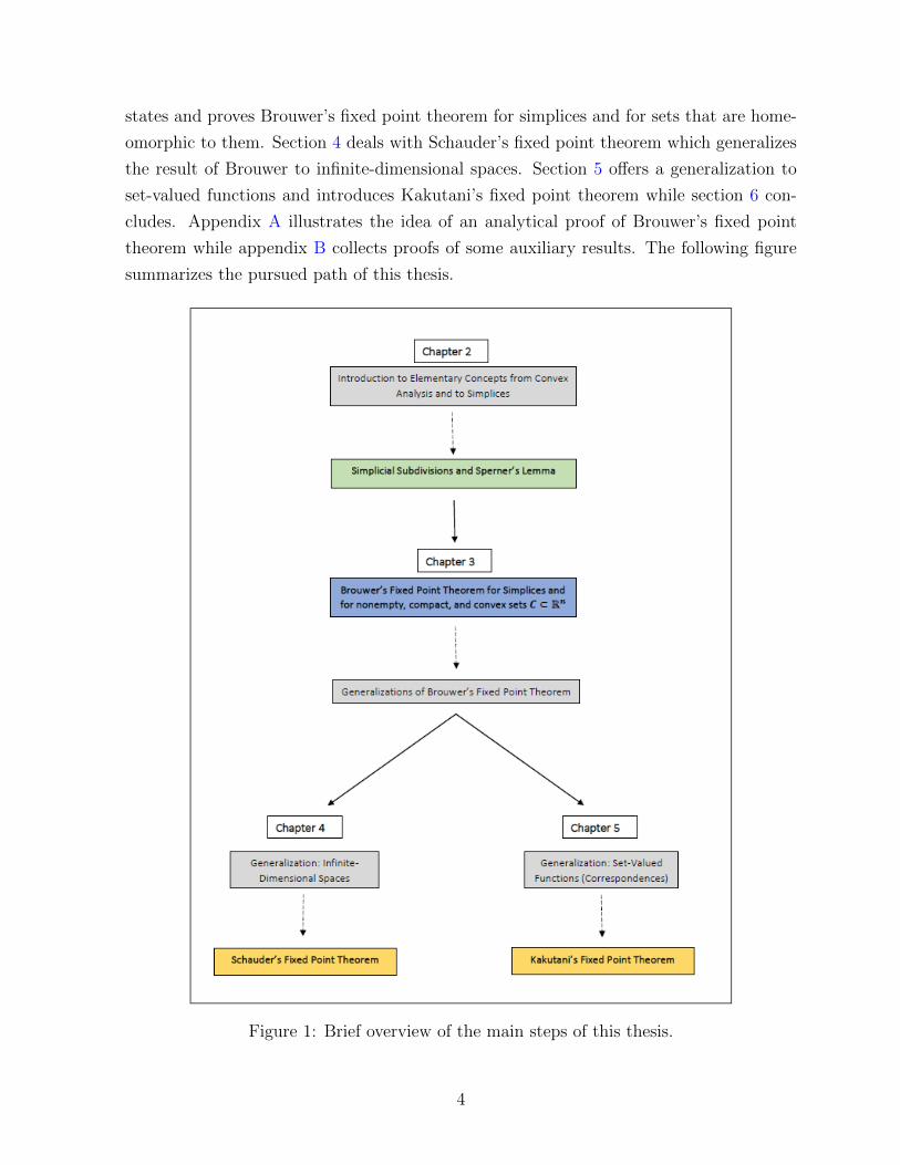


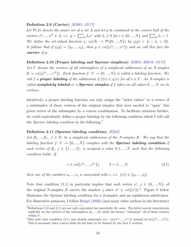


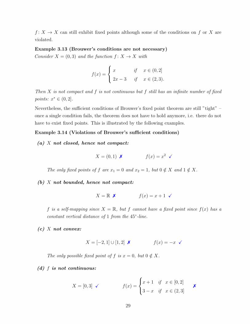

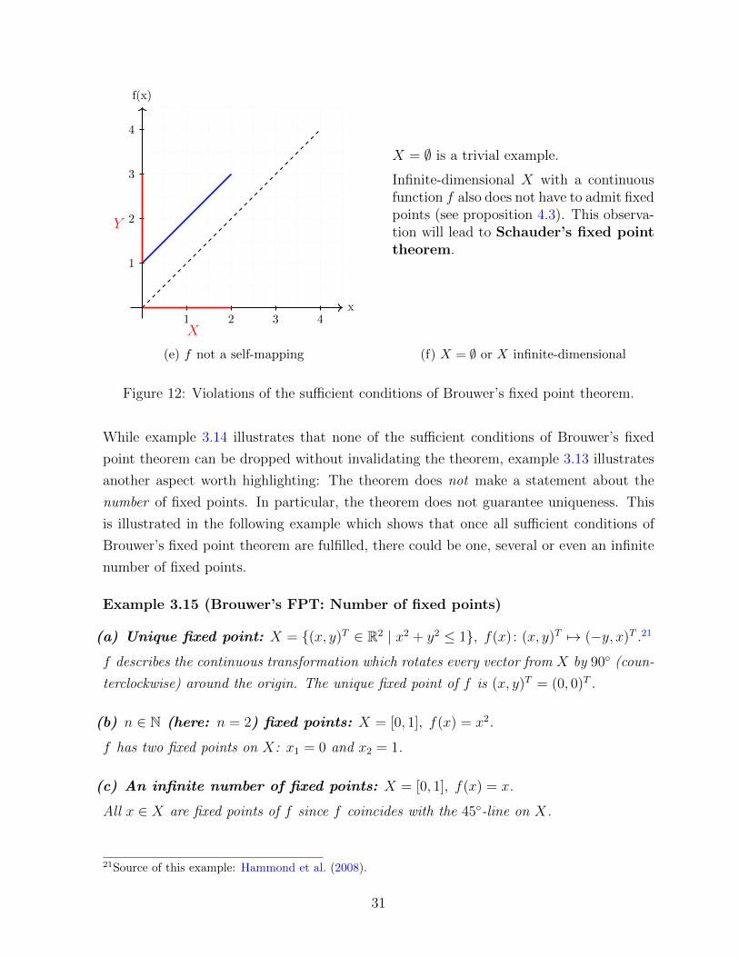

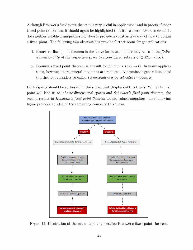


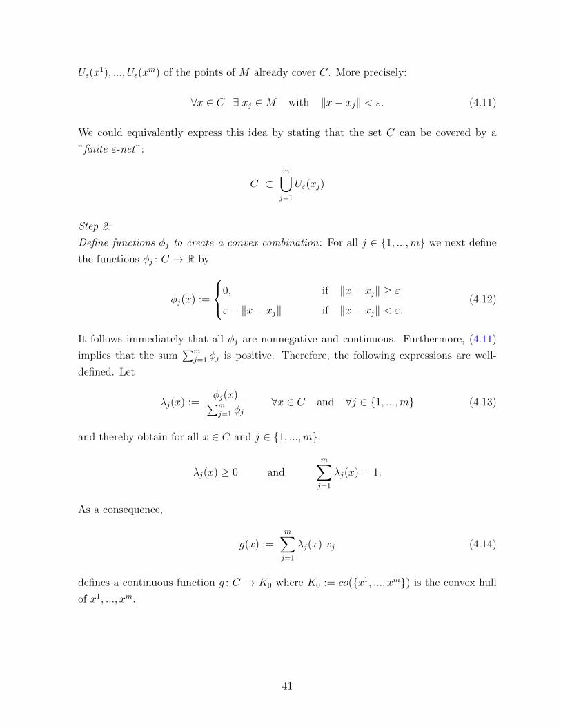


![Several Fixed Point Theorems on Partially Ordered Banach ... · point. Tarski’s Fixed Point Theorem on chain-complete lattice for single-valued mappings (see [12]) initiated a new](https://static.documents.pub/doc/80x56/5fdbb3bb000013674944e8db/several-fixed-point-theorems-on-partially-ordered-banach-point-tarskias-fixed.jpg)


