M¨ alardalen University Doctoral Thesis No.9 Flexible Scheduling for Media Processing in Resource Constrained Real-Time Systems Damir Isovi´ c November 2004 Department of Computer Science and Engineering M¨ alardalen University V¨ aster˚ as, Sweden
Transcript
Malardalen University Doctoral ThesisNo.9
Flexible Scheduling for MediaProcessing in ResourceConstrained Real-Time
Systems
Damir Isovic
November 2004
Department of Computer Science and EngineeringMalardalen University
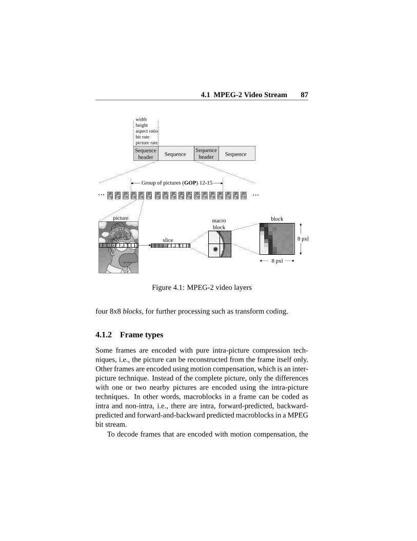
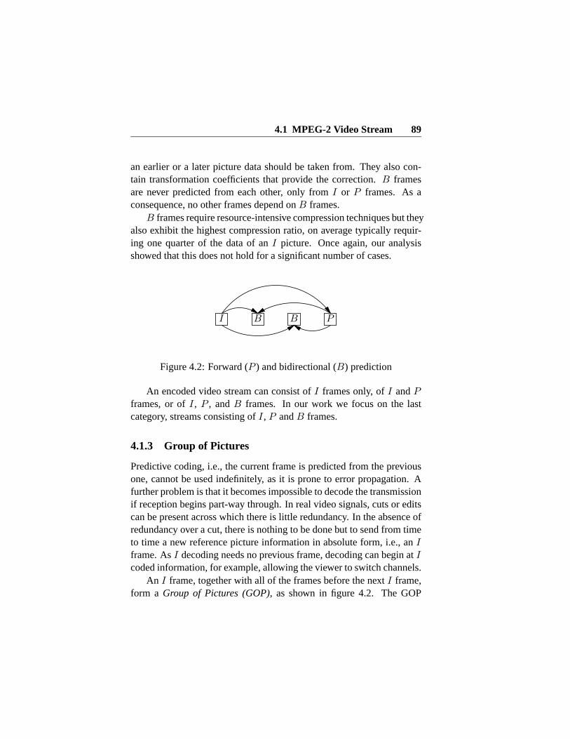
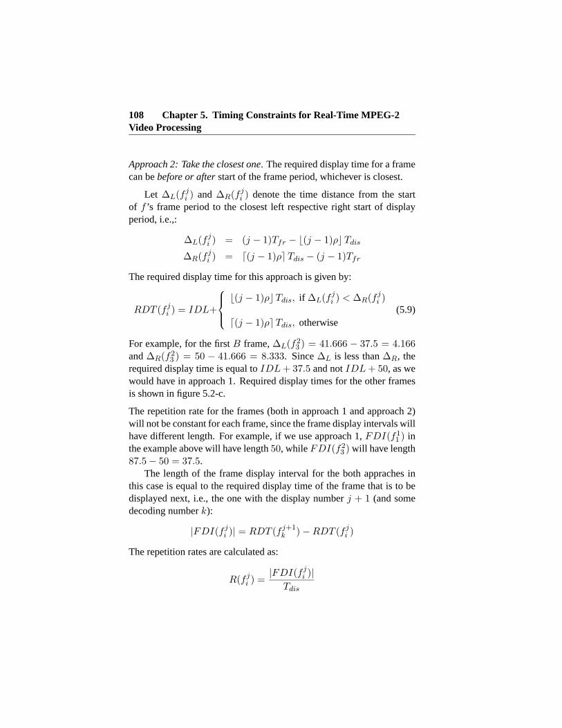
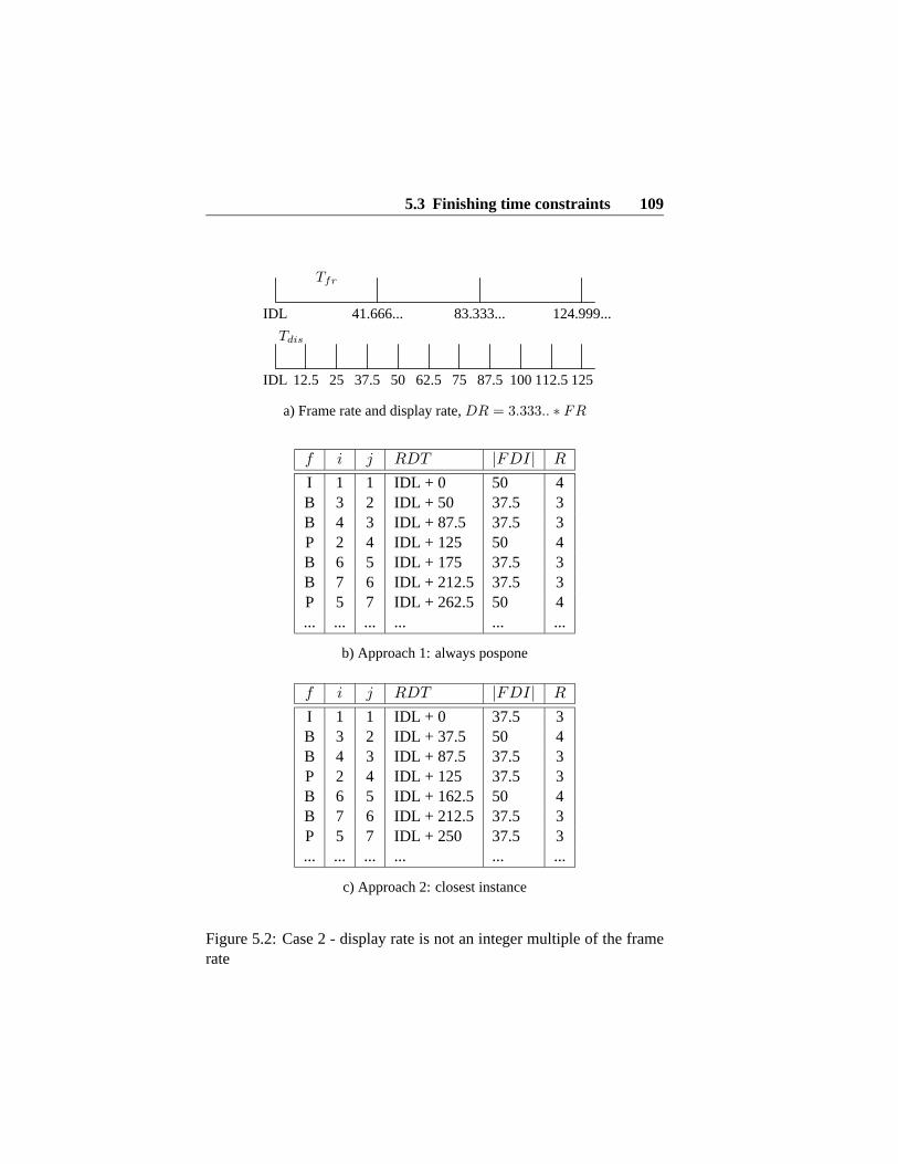
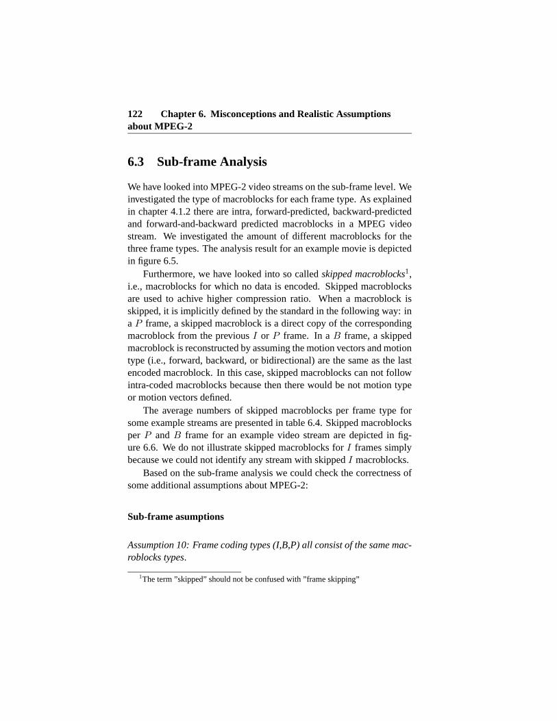
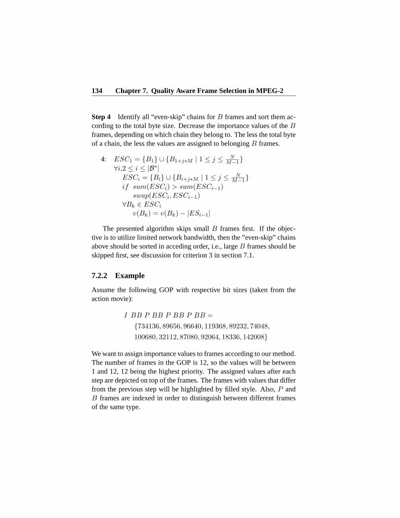
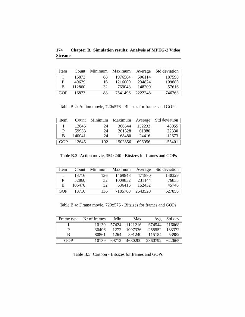
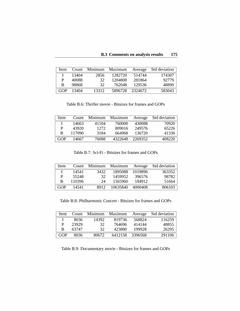
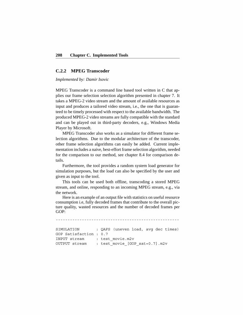
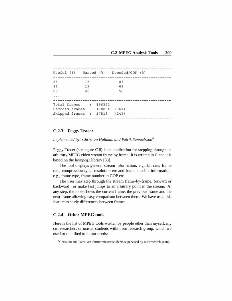
The MPEG-2 standard for video coding is predominant in consumerelectronics for DVD players, digital satellite receivers, and TVs today.MPEG-2 processing puts high demands on audio/video quality, which isachieved by continuous and synchronized playout without interrupts. Atthe same time, there are restrictions on the storage media, e.g.., limitedsize of a DVD disc, communication media, e.g., limited bandwidth ofthe Internet, display devices, e.g., the processing power, memory andbattery life of pocket PCs or video mobile phones, and finally the users,i.e., humans ability of perceiving motion. If the available resources arenot sufficient to process a full-size MPEG-2 video, then video streamadaptation must take place. However, this should be done carefully,since in high quality devices, drops in perceived video quality are nottolerated by consumers.
We propose real-time methods for resource reservation of MPEG-2video stream processing and introduce flexible scheduling mechanismsfor video decoding. Our method is a mixed offline and online approachfor scheduling of periodic, aperiodic and sporadic tasks, based on slotshifting. We use the offline part of slot shifting to eliminate all typesof complex task constraints before the runtime of the system. Then,we propose an online guarantee algorithm for dealing with dynamicallyarriving tasks. Aperiodic and sporadic tasks are incorporated into theoffline schedule by making use of the unused resources and leeways inthe schedule. Sporadic tasks are guaranteed offline for the worst-casearrival patterns and scheduled online, where an online algorithm keeps
i
ii
track of arrivals of instances of sporadic tasks to reduce pessimism aboutfuture sporadic arrivals and improve response times and acceptance offirm aperiodic tasks. At runtime, our mechanism ensures feasible exe-cution of tasks with complex constraints in the presence of additionaltasks or overloads.
We use the scheduling and resource reservation mechanism aboveto flexibly process MPEG-2 video streams. First, we present resultsfrom a study of realistic MPEG-2 video streams to analyze the valid-ity of common assumptions for software decoding and identify a num-ber of misconceptions. Then, we identify constraints imposed by framebuffer handling and discuss their implications on the decoding architec-ture and timing. Furthermore, we propose realistic timing constraintsdemanded by high quality MPEG-2 software video decoding. Based onthese, we present a MPEG-2 video frame selection algorithm with focuson high video quality perceived by the users, which fully utilize limitedresources. Given that not all frames in a stream can be processed, itselects those which will provide the best picture quality while matchingthe available resources, starting only such decoding, which is guaran-teed to be completed. As a final result, we provide a real-time methodfor flexible scheduling of media processing in resource constrained sys-tem. Results from study based on realistic MPEG-2 video underline theeffectiveness of our approach.
To my beloved wife Eminaand daughter Hanna
Preface
After finishing my Licentiate thesis in 2001, as a part of my graduatestudies, I realized how confusing this exam was to other people. Noteven many Swedes were familiar with this odd degree. Is it the same as”master degree” in the USA? As ”magistrat” in my country of origin,Bosnia and Hercegovina? I have tried to explain it for people with moreor less success by describing it as ”half-PhD” or a ”super-engineer”exam. I do not have that problem any more – ”Doctor of Philosophy”sounds pretty much the same all over the world!
The journey here was not easy. Without support of many people, thiswork, probably, would not have been possible. I am grateful to them all,not only for their technical support, but also good time I have sharedwith them. Here, I would like to express my gratitude to all (and pleaseforgive me if I forget somebody, it is getting really late:)
First of all, my family: my greatest thanks go to my beloved wifeEmina and my daughter Hanna for their love and support during the longnight hours when completing this thesis. I am grateful to my parents andfamily for always encouraging me to pursue my ideas and desires andfor their unfailing support and love throughout my entire education. Iwould never make it without you.
I would like to thank my supervisor Gerhard Fohler for believing inme and leading me all the way to this degree. Thank you, Gerhard, foralways pushing me to my limits. It might not have been fun all the time,but now I know it was the right way to go. Doing anything less than myabsolute best would have never given me this type of satisfaction that I
v
vi
feel now. I appreciate it a lot.My deepest gratitude goes to the rest of the SALSART group: Radu,
Tomas, Larisa, and Pau, for the great time we spent together, no only inmeeting rooms, but also at pubs. It’s been a real pleasure to work withyou.
I also want to thank my colleagues at the Department of ComputerScience at Malardalen University, especially the members of the SystemDesign Lab. Thanks, Ylva, for giving me instructions how to describemy research in a popular-scientific way. Without you ”massacring” thefirst draft of my proposed description, I would never be able to explainto my parents what I do.
During the last phase of my graduate studies, I’ve spent some time atthe University of North Carolina at Chapel Hill. I would like to expressmy gratitude to all members of the department, especially to Sanjoy andhis family, and Shelby, for taking such a good care of me, Emina andHanna during our visit, and to Ketan for the technical discussions andhelp. Thanks to Ketan’s almost ridiculously extensive knowledge aboutthe darkest secrets of MPEG, many sub-frame level issues became moreclear.
I would also like to express my gratitude to all the people that Icooperated with in one way or another, especially people form ReTiSlab in Pisa: Giorgio, Peppe, Marco, Paolo, and peopple from the PhilipsResearch, Liesbeth and Clemens. Thank you for fruitfull discussionsand to the reviewers for helpful comments.
Finally, a piece of advice for all graduate students: do not wait withwriting the preface until the last day before printing the thesis, as I did!After all the pain and the agony you are going to suffer while ”just writ-ing it down”, believe me, you are not in the right mood to thank people:)
Damir IsovicVasteras, October 17, 2004, 02:25
Publications
I have authored or co-authored the following publications:
Journals
• Damir Isovic, Gerhard Fohler and Liesbeth Steffens: Real-timeissues of MPEG-2 playout in resource constrained systems, Inter-national Journal on Embedded Systems, June 2004.
Articles in collection
• Damir Isovic and Christer Norstrom: Requirements for Real-TimeComponents, Building Reliable Component-Based Systems, edi-tors: Ivica Crnkovic and Magnus Larsson, Artech House Publish-ers, 2002.
Conferences and workshops
• Damir Isovic and Gerhard Fohler: Quality aware MPEG-2 streamadaptation in resource constrained systems, 16th Euromicro Con-ference on Real-time Systems (ECRTS ’04), Catania, Sicily, Italy,July 2004.
• Damir Isovic, Gerhard Fohler and Liesbeth Steffens: Timing con-straints of MPEG-2 decoding for high quality video: misconcep-tions and realistic assumptions, Proceedings of the 15th Euromi-
vii
viii
cro Conference on Real-Time Systems (ECRTS ’03), Porto, Por-tugal, July 2003.
• Damir Isovic, Gerhard Fohler and Liesbeth Steffens: Some Mis-conceptions about Temporal Constraints of MPEG-2 Video De-coding, WiP of the 23rd IEEE International Real-Time SystemsSymposium (RTSS ’03), Austin, Texas, USA, December 2002.
• Damir Isovic and Christer Norstrom: Components in Real-TimeSystems, The 8th International Conference on Real-Time Com-puting Systems and Applications (RTCSA ’02), Tokyo, Japan,March 2002.
• Gerhard Fohler, Damir Isovic, Tomas Lennvall and Roger Vuolle:SALSART - A Web Based Cooperative Environment for OfflineReal-time Schedule Design, 10th Euromicro Workshop on Paral-lel, Distributed and Network-based Processing (PDP ’02), GranCanaria, Spain, January 2002.
• Damir Isovic and Gerhard Fohler: Efficient Scheduling of Spo-radic, Aperiodic, and Periodic Tasks with Complex Constraints,Proc. of the 21st IEEE Real-Time Systems Symposium (RTSS’00), Walt Disney World, Orlando, Florida, USA, November 2000.
• Damir Isovic, Markus Lindgren and Ivica Crnkovic: System De-velopment with Real-Time Components, Proc. of ECOOP 2000Workshop 22 - Pervasive Component-based systems, Sophia An-tipolis and Cannes, France, June 2000.
• Damir Isovic and Gerhard Fohler: Online Handling of Firm Ape-riodic Tasks in Time Triggered Systems, 12th EUROMICRO Con-ference on Real-Time Systems (ECRTS ’00), Stockholm, Swe-den, June 2000.
• Damir Isovic and Gerhard Fohler: Handling Sporadic Tasks inOff-line Scheduled Distributed Real-Time Systems, 11th EUROMI-CRO Conference on Real-Time Systems (ECRTS ’99), York, Eng-land, July 1999.
ix
Technical reports
• Damir Isovic, Gerhard Fohler: Analysis of MPEG-2 Video Streams,MRTC Report , Malardalen Real-Time Research Centre, MalardalenUniversity, August 2002
• Damir Isovic, Gerhard Fohler: Resource Aware MPEG-2 PlayoutUsing Real-time Scheduling, Technical Report , Malardalen Real-Time Research Centre, March 2001.
• Damir Isovic, Christer Norstrm: Components in Real-Time Sys-tems, MRTC Report, Malardalen Real-Time Research Centre, MalardalenUniversity, December 2001.
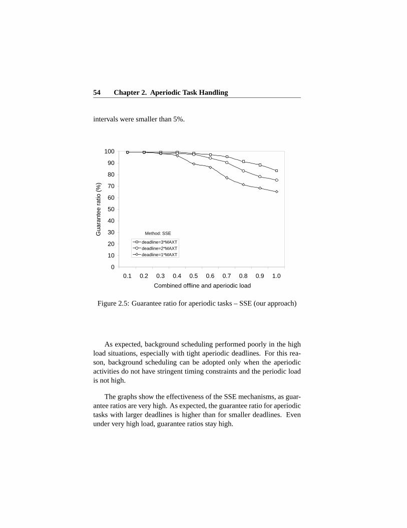
• Damir Isovic, Gerhard Fohler: Simulation Analysis of Sporadicand Aperiodic Task Handling, MRTC Report ISSN 1404-3041ISRN MDH-MRTC-38/2001-1-SE, Malardalen Real-Time ResearchCentre, Malardalen University, May 2001
Licentiate Thesis
• Damir Isovic: Handling Sporadic Tasks in Real-time Systems -Combined Offline and Online Approach, Licentiate Thesis, MalardalenUniversity Press, June 2001.
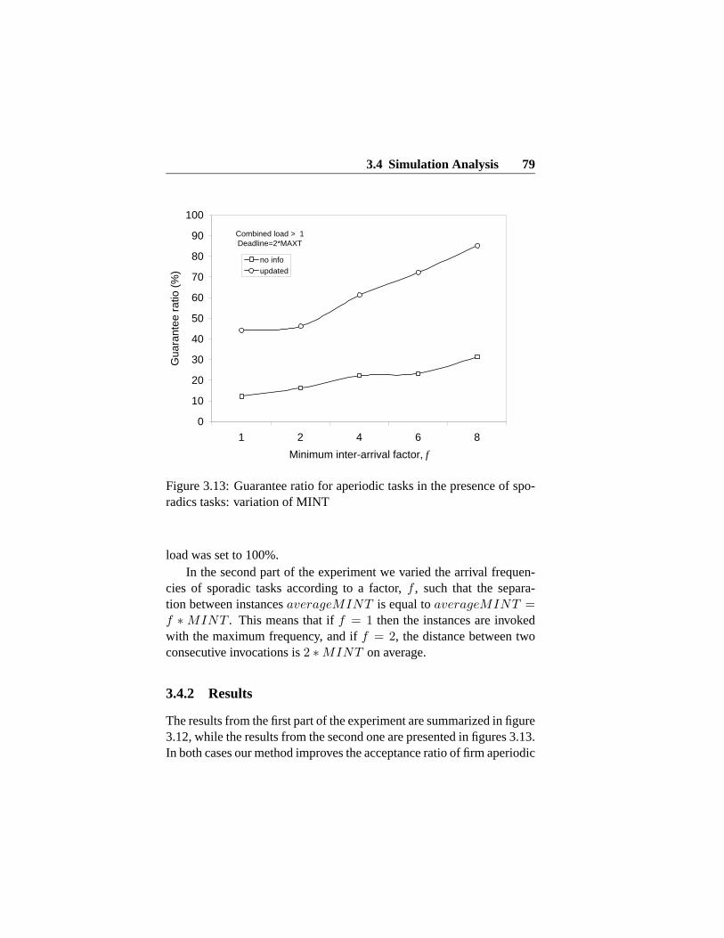
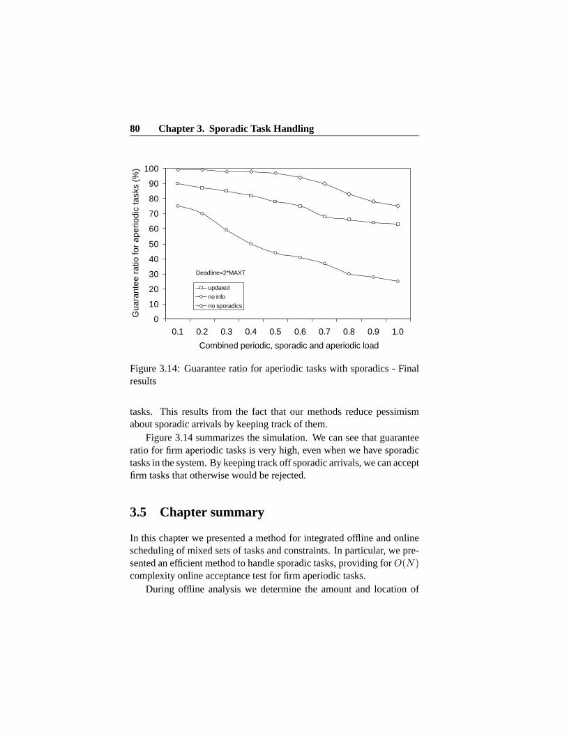
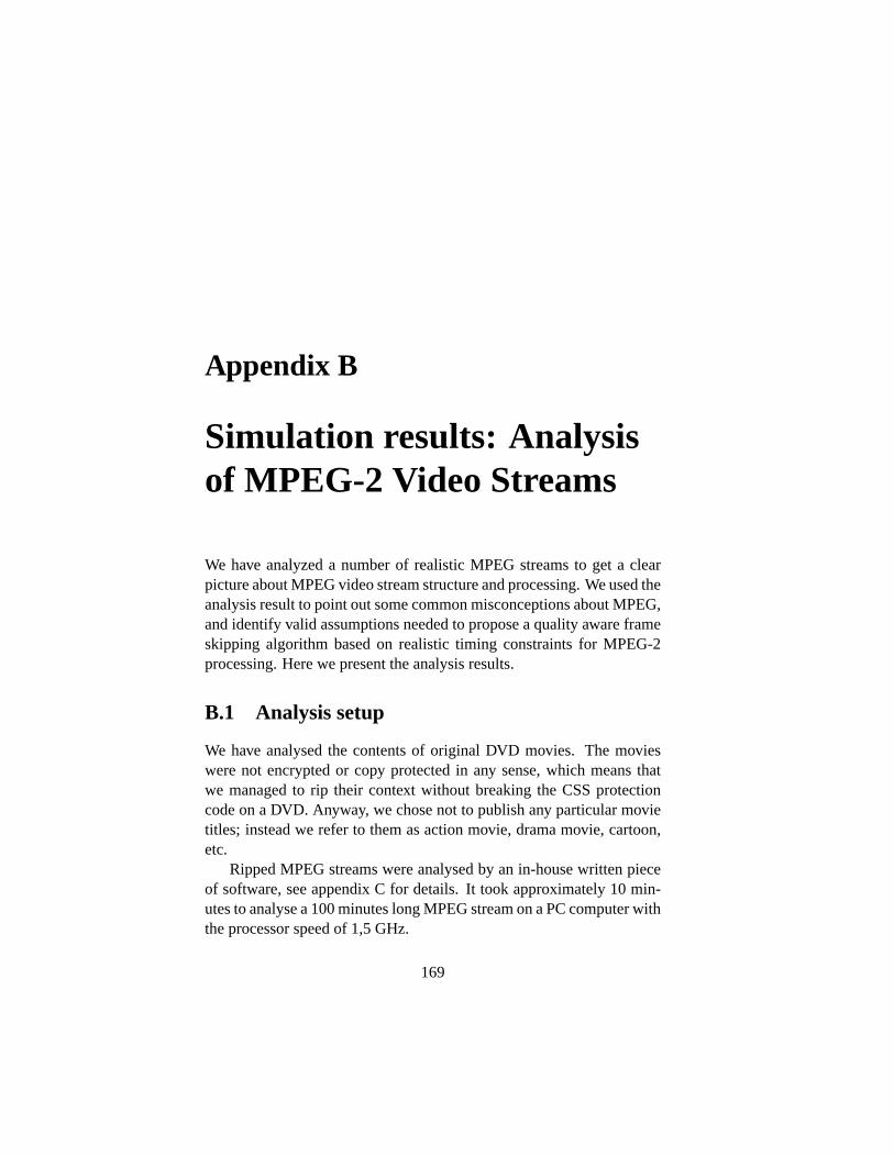
A.4 Guarantee ratio for aperiodic tasks – Background . . . . 163A.5 Guarantee ratio for aperiodic tasks – SSE (our approach) 163A.6 Guarantee ratio for aperiodic tasks in the presence of
sporadics tasks, dl=MAX: load variation . . . . . . . . . 165A.7 Guarantee ratio for aperiodic tasks in the presence of
sporadics tasks, dl=2*MAXT: load variation . . . . . . . 165A.8 Guarantee ratio for aperiodic tasks in the presence of
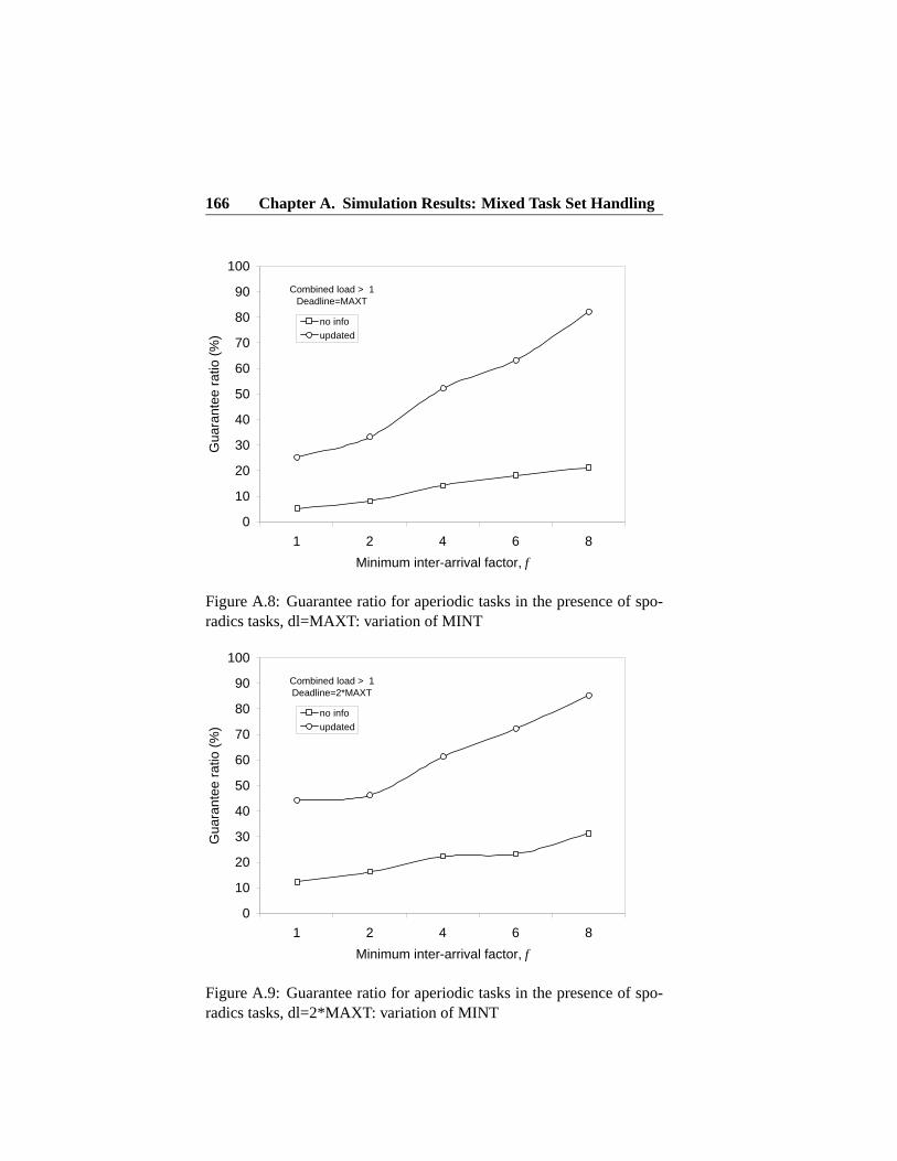
sporadics tasks, dl=MAXT: variation of MINT . . . . . 166A.9 Guarantee ratio for aperiodic tasks in the presence of
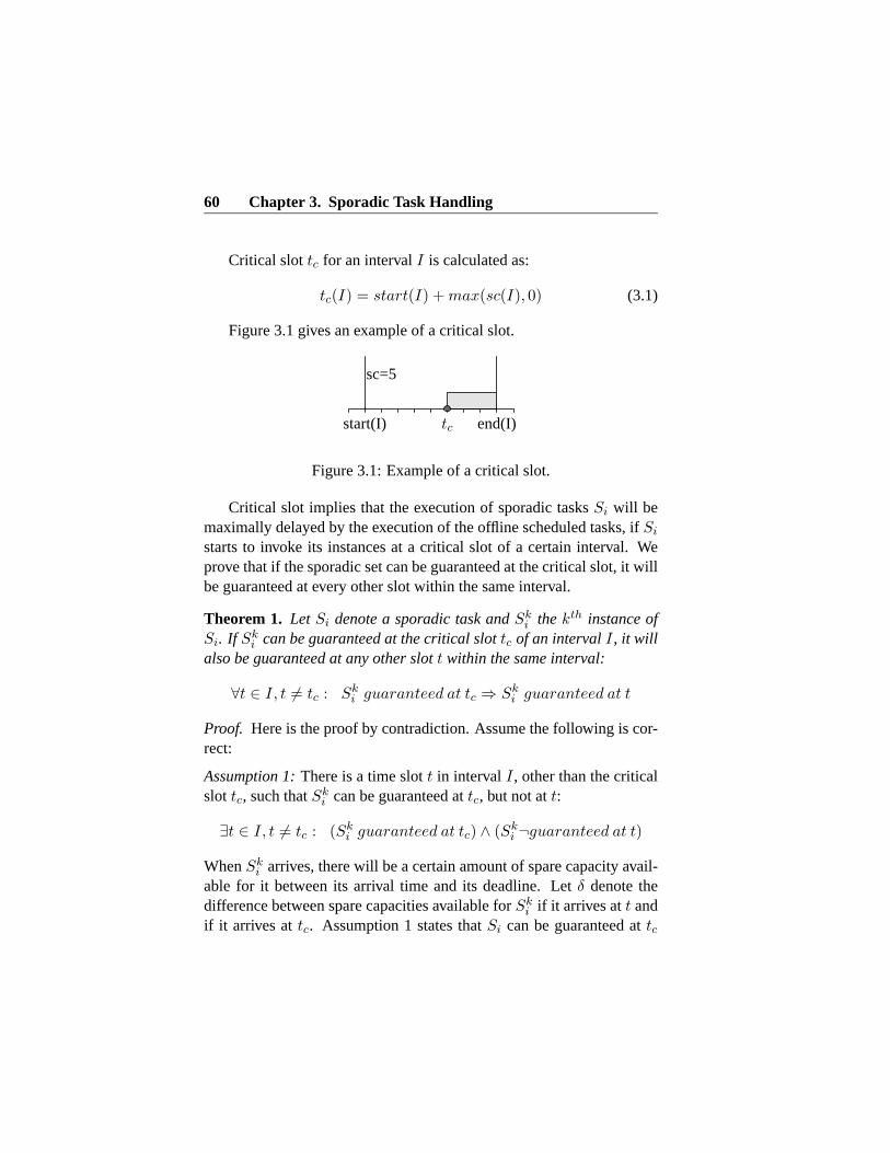
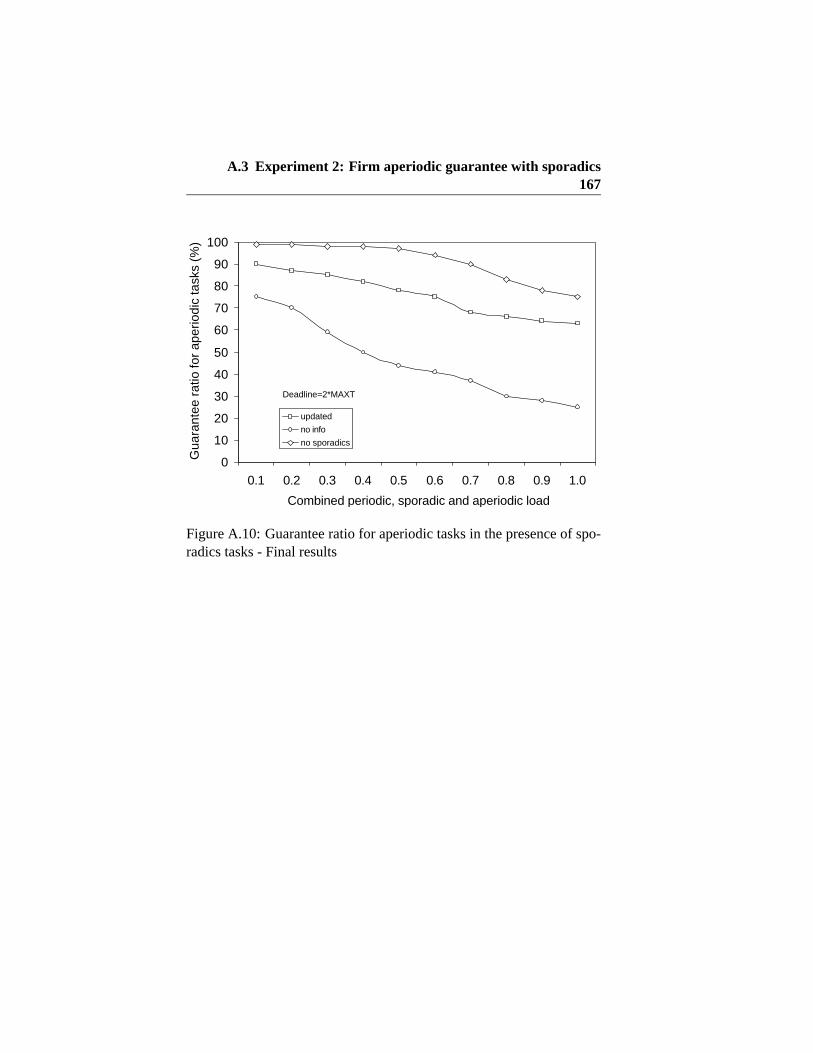
sporadics tasks, dl=2*MAXT: variation of MINT . . . . 166A.10 Guarantee ratio for aperiodic tasks in the presence of
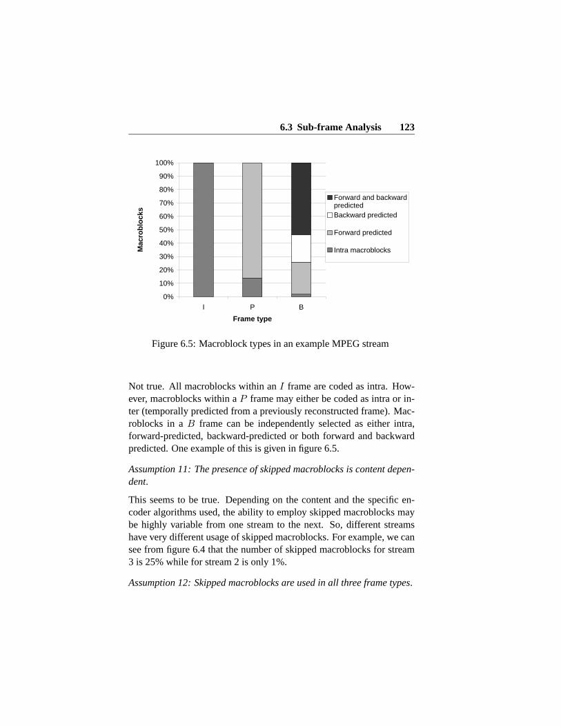
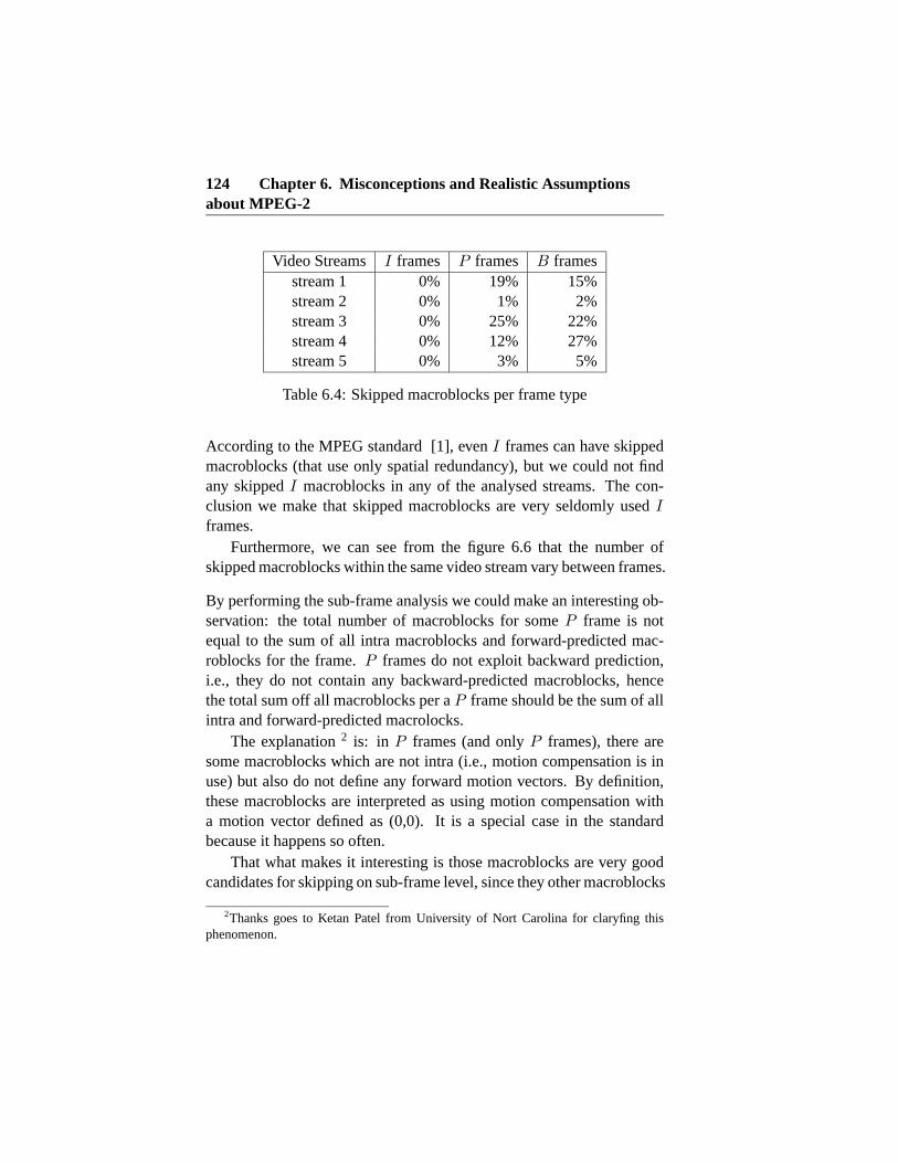
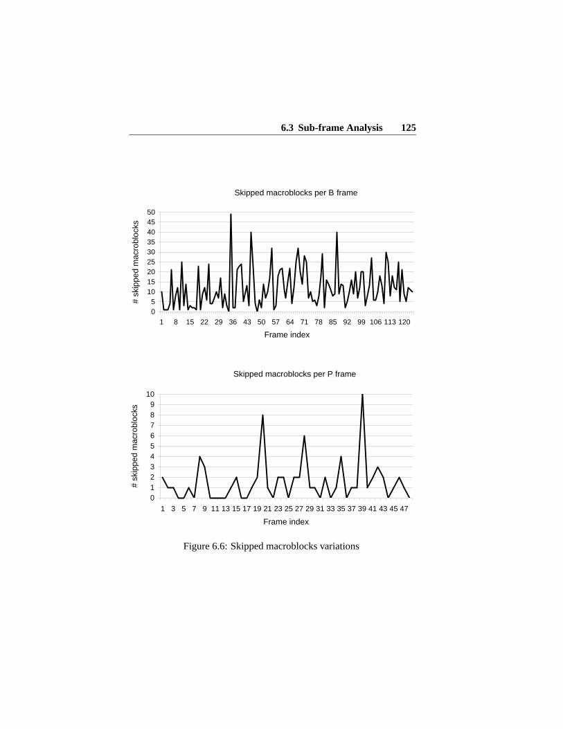
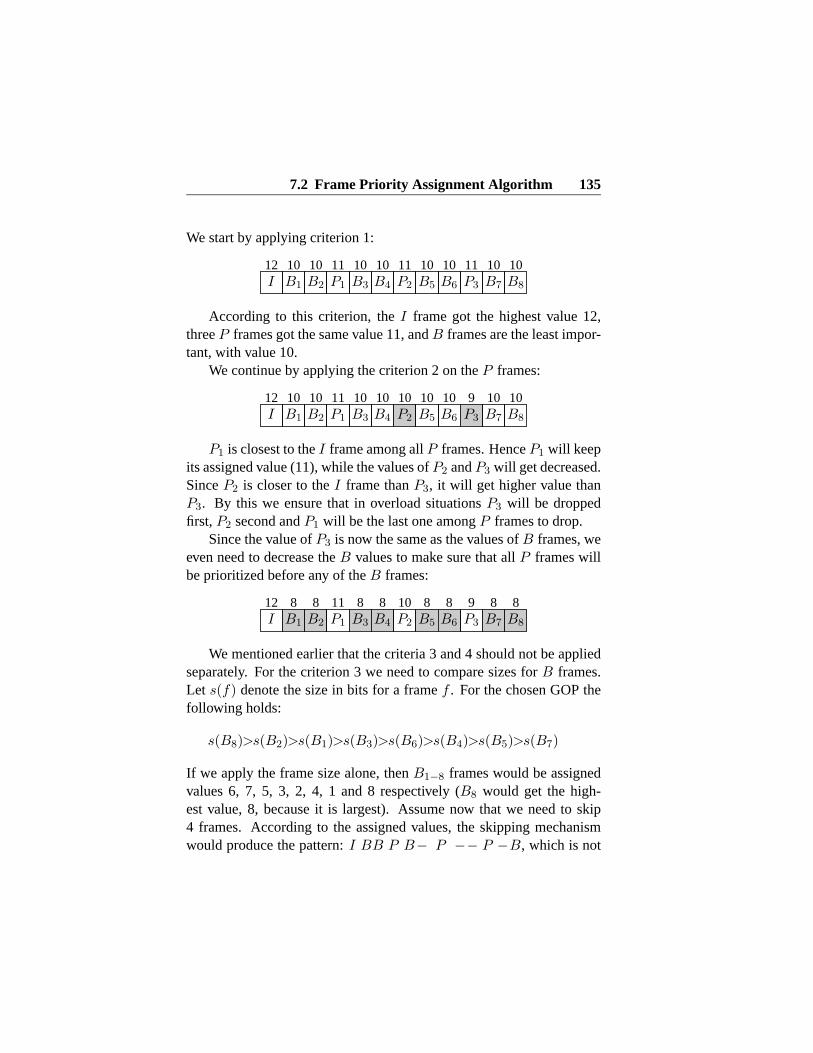
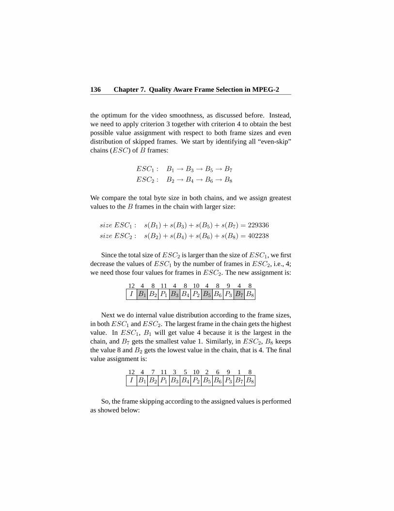
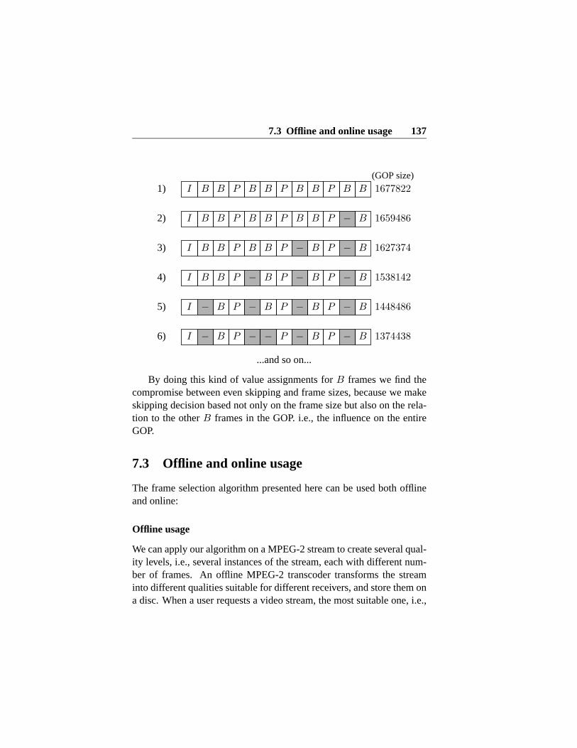
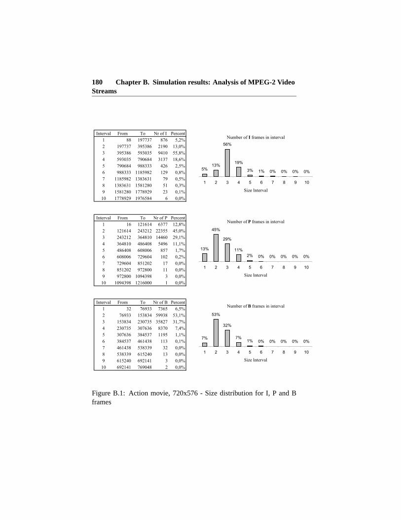
B.1 Action movie, 720x576 - Size distribution for I, P andB frames . . . . . . . . . . . . . . . . . . . . . . . . . . 180
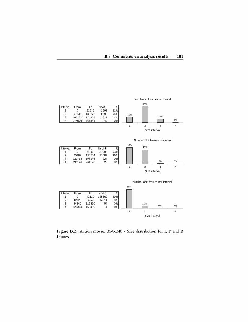
B.2 Action movie, 354x240 - Size distribution for I, P andB frames . . . . . . . . . . . . . . . . . . . . . . . . . . 181
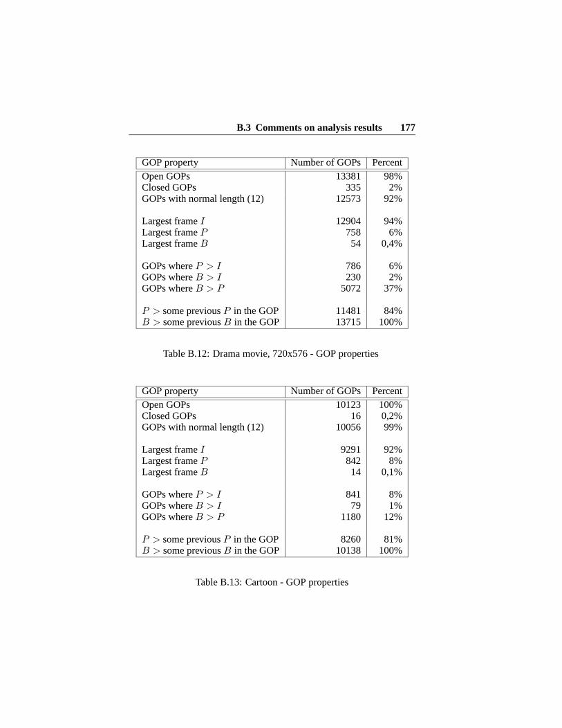
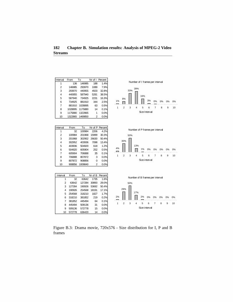
B.3 Drama movie, 720x576 - Size distribution for I, P andB frames . . . . . . . . . . . . . . . . . . . . . . . . . . 182
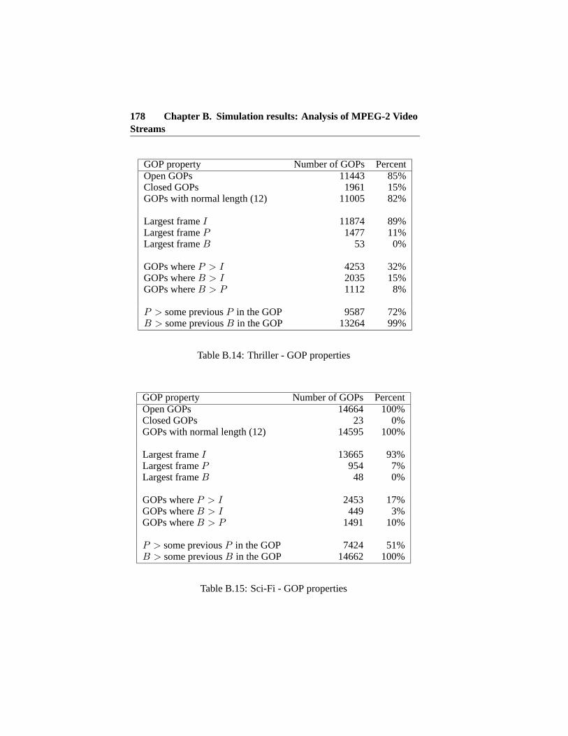
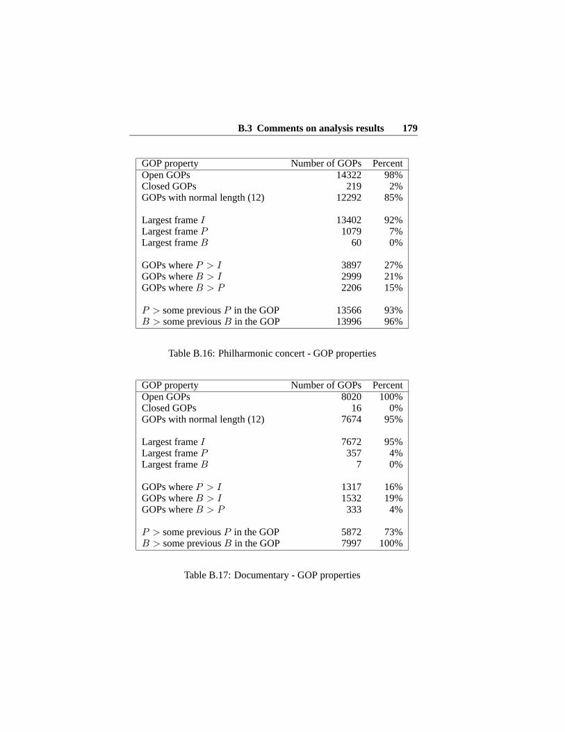
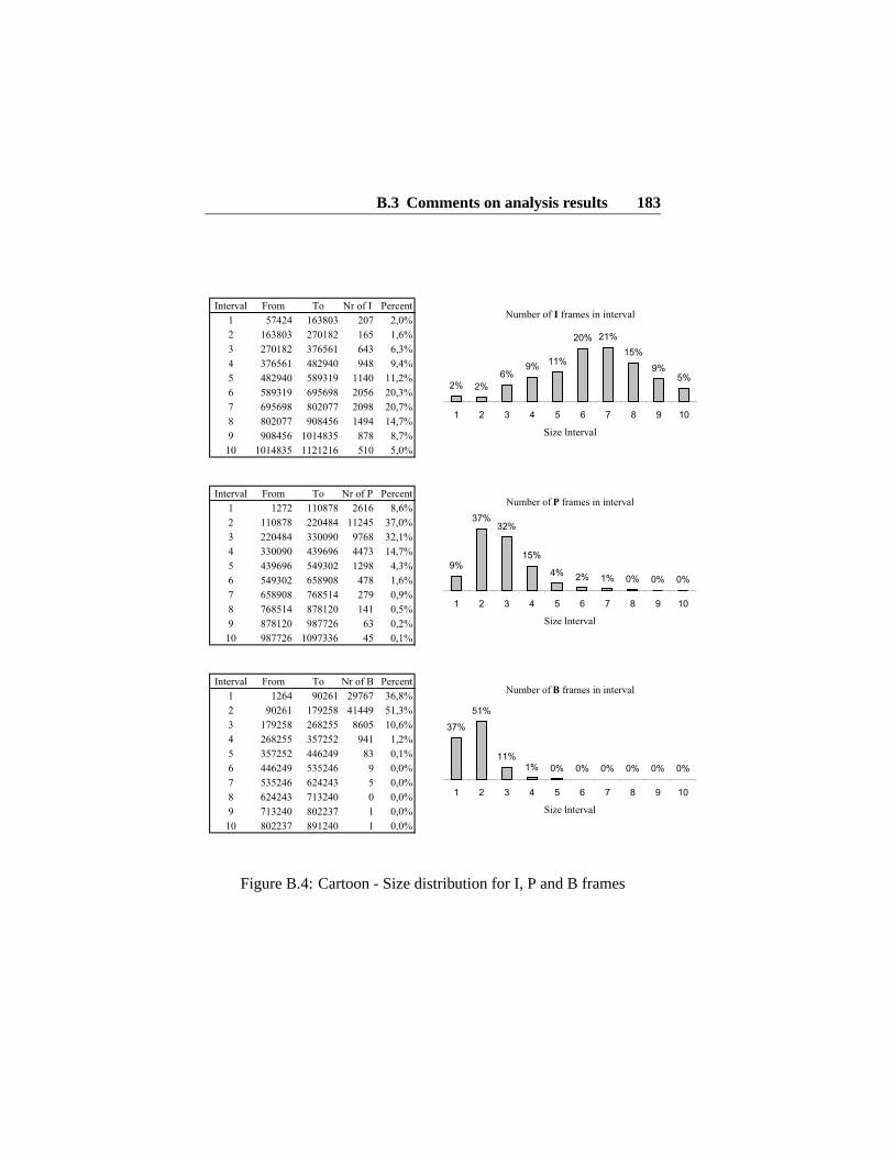
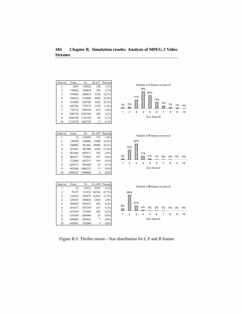
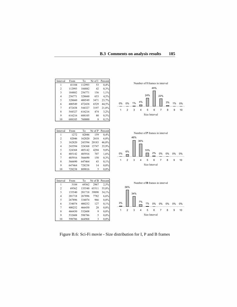
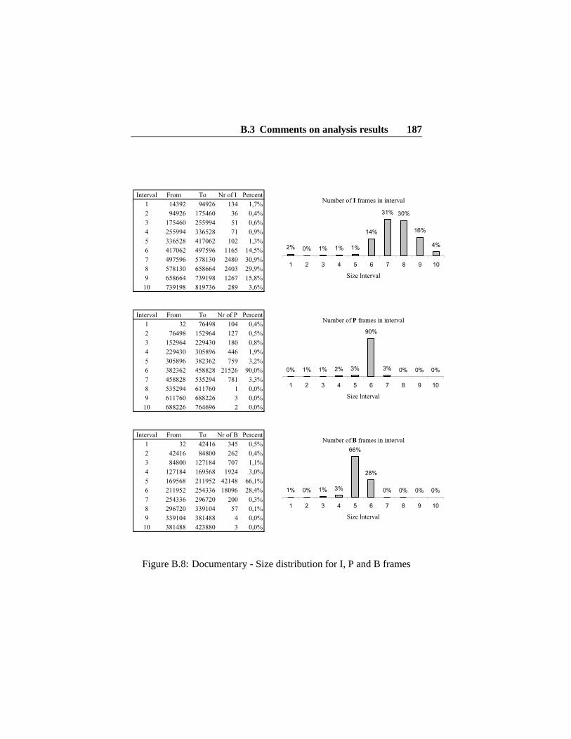
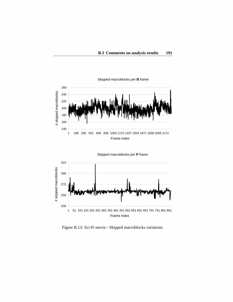
B.4 Cartoon - Size distribution for I, P and B frames . . . . . 183B.5 Thriller movie - Size distribution for I, P and B frames . 184B.6 Sci-Fi movie - Size distribution for I, P and B frames . . 185B.7 Philharmonic - Size distribution for I, P and B frames . . 186B.8 Documentary - Size distribution for I, P and B frames . . 187B.9 Action movie - Macroblock types . . . . . . . . . . . . 188B.10 Drama movie - Macroblock types . . . . . . . . . . . . 188B.11 Action movie - Skipped macroblocks variations . . . . . 189B.12 Drama movie - Skipped macroblocks variations . . . . . 190
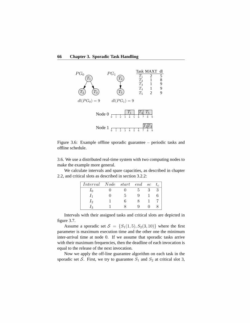
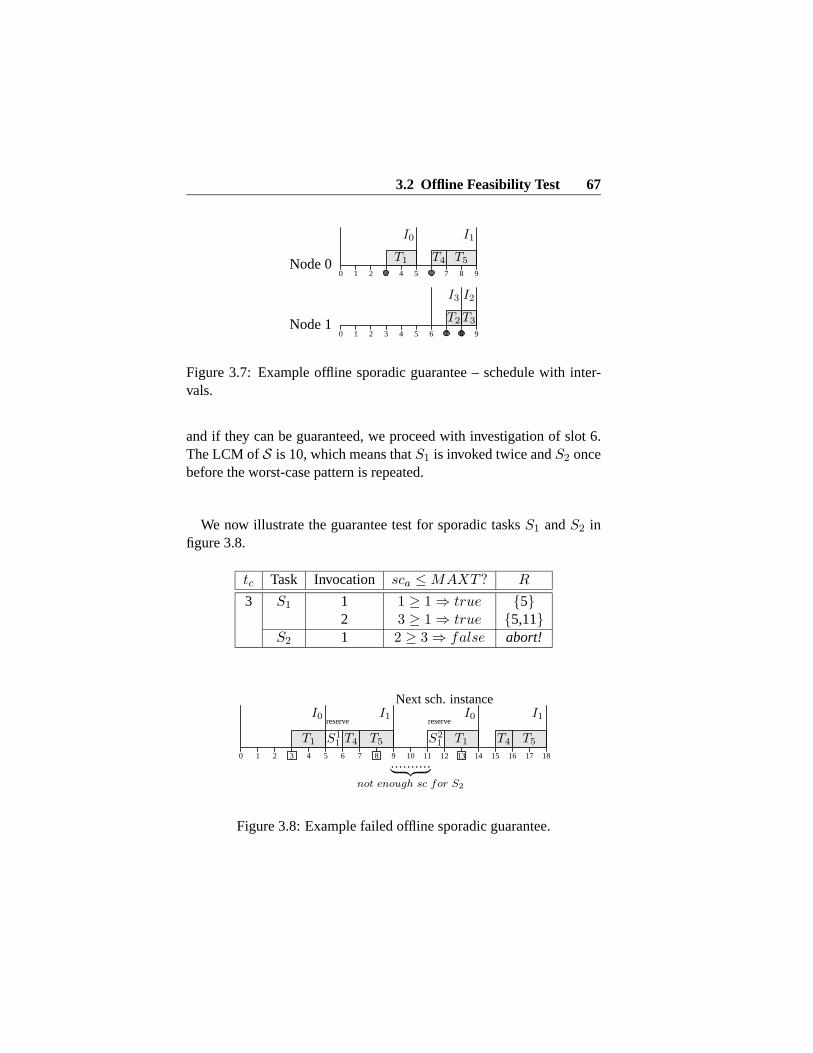
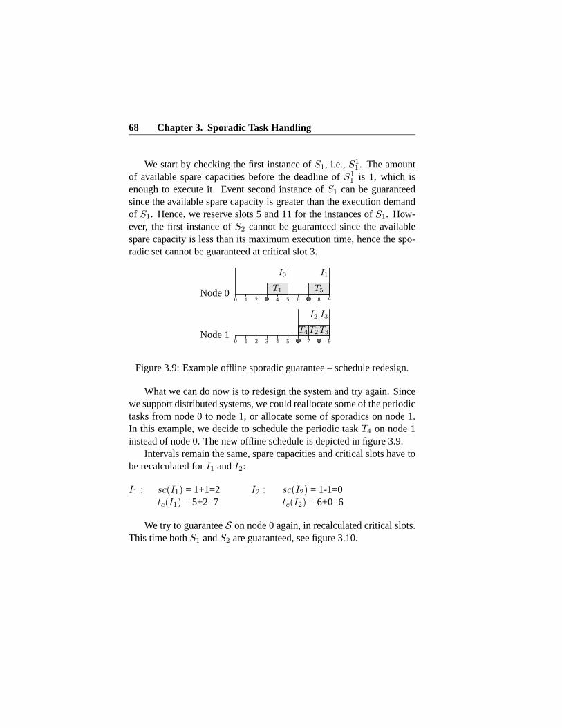
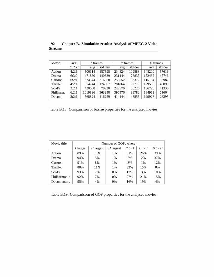
B.18 Comparrison of bitsize properties for the analysed movies192B.19 Comparisson of GOP properties for the analysed movies 192
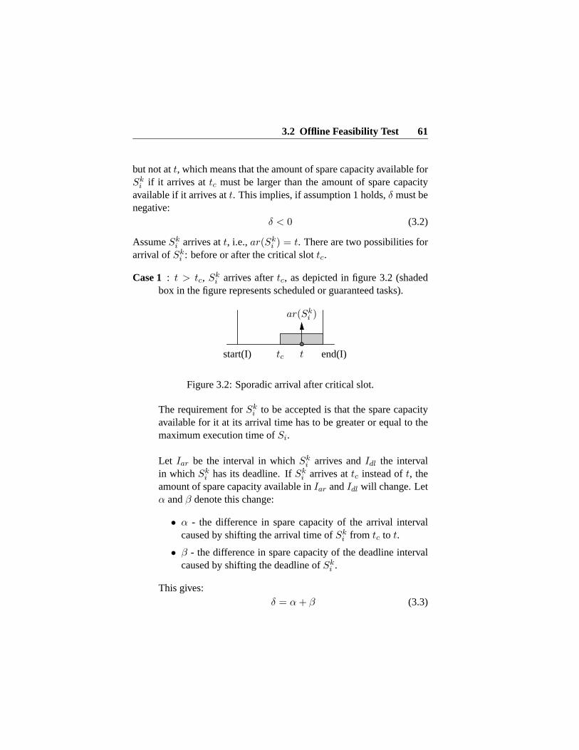
Chapter 1
Introduction
In a near future, most of the existing analog home entertainment de-vices, such as TVs and VCRs, will be replaced by corresponding digitalproducts. In 2008, all analog television broadcasting in Sweden will bereplaced by digital signals that better utilize the communication mediaand provide for a greater variety of TV channels and interactive servicesthat are not possible in the analog domain. Examples of other sourcesof digital video and audio include DVDs, Video CDs, and Internet.
Compared to the analog domain, digital media introduces additionaland different requirements on the environment. At the same time, thereare restrictions on the communication and storage media, display de-vices and users. In their original form, digital multimedia streams arevery big in size, while the storage and the communication media havelimited resources. Thus, media files must be compressed before beingstored on e.g., a DVD, or transmitted through a network, e.g., the In-ternet. MPEG – Moving Picture Expert Group – is the most popularcompression technique for digital video and audio today. It defines agroup of standards for digital storage and distribution of video and au-dio. Currently, the most used standard of the MPEG group is MPEG-2,used in e.g., DVDs or digital satellite broadcasting.
Display devices are also restricted, e.g., with respect to processingpower, memory, and battery life. For instance, the processing power of
1
2 Chapter 1. Introduction
hand held devices, such as pocket PCs or video mobile phones, is notsufficient to play out a full-size video stream without impairing videoquality.
Additional requirements are imposed by the user, e.g., human’s abil-ity of perceiving motion. An MPEG-2 movie is a stream of still imagesdisplayed after each other fast enough that the human eye cannot no-tice the delay between consecutive pictures, i.e., the stream is perceivedas motion. For example, a DVD movie is displayed on a TV set witha rate of approximately 25 frames per second. This implies there are40 milliseconds per picture available to read the picture from the disc,decode its contents and display it on the screen. Delays in this processmay result in severe video quality degradation of the played stream.
Matching video processing requirements to system limitations
One way of matching some of the requirements imposed by process-ing of MPEG-2 streams with the limitations of the target systems is touse dedicated hardware solutions. However, dedicated hardware cannotcompensate for the limitations in the network bandwidth: in the case ofvideo streaming, it does not matter if there is enough processing powerto decode a full-size MPEG-2 video stream if there is not enough net-work bandwidth available for its transmission. Besides, within the nextfew years, MPEG-2 decoding will move from dedicated hardware tosoftware, for reasons of cost, rapid upgradeability, and configurability.While being more flexible, software solutions are more irregular, sincevideo processing will compete for the CPU with other applications inthe system. Besides, cost-effective software media processing requiresa high average resource utilization, leading to instability upon worst-case resource demands. Consequently, we need methods for decreasingthe load required by media applications in resource constrained systems.
There are three ways for compensating for limited resources for me-dia processing: decrease bit rate of the stream, use degraded decodingalgorithm and frame skipping, as depicted in figure 1.1. Which methodsshould be used depends on the situation. If the network bandwidth islimited, the streaming server can replace the current stream with a lower
3
Network
Stream sources Display devices
Need for stream adaptation
Limited NW bandwidth
Degradeddecoding algorithm
Frameskipping
methodsDecreased
stream bitrate
Videostream
Limitedprocessingpower
Figure 1.1: MPEG-2 video stream adaptation under limited resources
bit rate alternative. If the processing power on the display device is anissue, then downgraded decoding algorithm that uses less CPU powercan be used.
The third apprach is frame skipping. It means if not all video framesin a MPEG-2 stream cannot be decoded due to limited resources, someframes are not decoded and displayed, i.e., they skipped. Frame skip-ping can be used in both cases above: it can take place both before send-ing the stream on the network, if the network bandwidth is restricted, oron the display device, if the processing power is limited.
In our work, we use the frame skipping approach with focus on highvideo quality perceived by the users.
4 Chapter 1. Introduction
Our approach
In this thesis, we propose a method for flexible scheduling of MPEG-2video stream processing in resource constrained systems. We use real-time methods for scheduling and resource reservation to fulfill the re-quirements of software MPEG-2 video decoding.
In the first part of this thesis we present scheduling mechanisms forintegrated offline and online scheduling, which we later apply to flexibleprocessing of MPEG-2 video decoding. The scheduling methods pre-sented here provide for easy access of the amount and the distribution ofavailable resources, needed to optimize the adaptation of video streamsupon limited resources. We show how to flexibly schedule mixed setsof tasks, i.e., periodic, aperiodic and sporadic, with simple and complexconstraints by using an integrated offline and online approach. Offlinescheduling methods can resolve many specific constraints but at the ex-pense of runtime flexibility, in particular inability to handle dynamicallyarriving tasks. Online scheduling provides for flexibility, but it might in-troduce a high overhead for resolving complex constraints, if even possi-ble. Our method is a combined offline and online approach. We use theoffline part of slot shifting, introduced by Fohler [30], to eliminate alltypes of complex constraints before the runtime of the system. Then wepropose a an online guarantee algorithm for dealing with dynamic tasks.Aperiodic and sporadic tasks, are incorporated into the offline scheduleby making use of the unused resources and leeways in the schedule. Atruntime, our mechanism ensures feasible execution of tasks with com-plex constraints in the presence of additional tasks or overloads.
In the second part of the thesis, we use the scheduling and avail-able resource reservation mechanisms from the first part of the thesisto flexibly schedule MPEG-2 video streams. First, we present resultsfrom a study of realistic MPEG-2 video streams to analyze the validityof common assumptions for software decoding and identify a number ofmisconceptions. Then, we identify constraints imposed by frame bufferhandling and discuss their implications on decoding architecture andtiming. Furthermore, we propose realistic timing constraints demandedby high quality MPEG-2 software video decoding. Based on these, we
1.1 Real-Time Systems Background 5
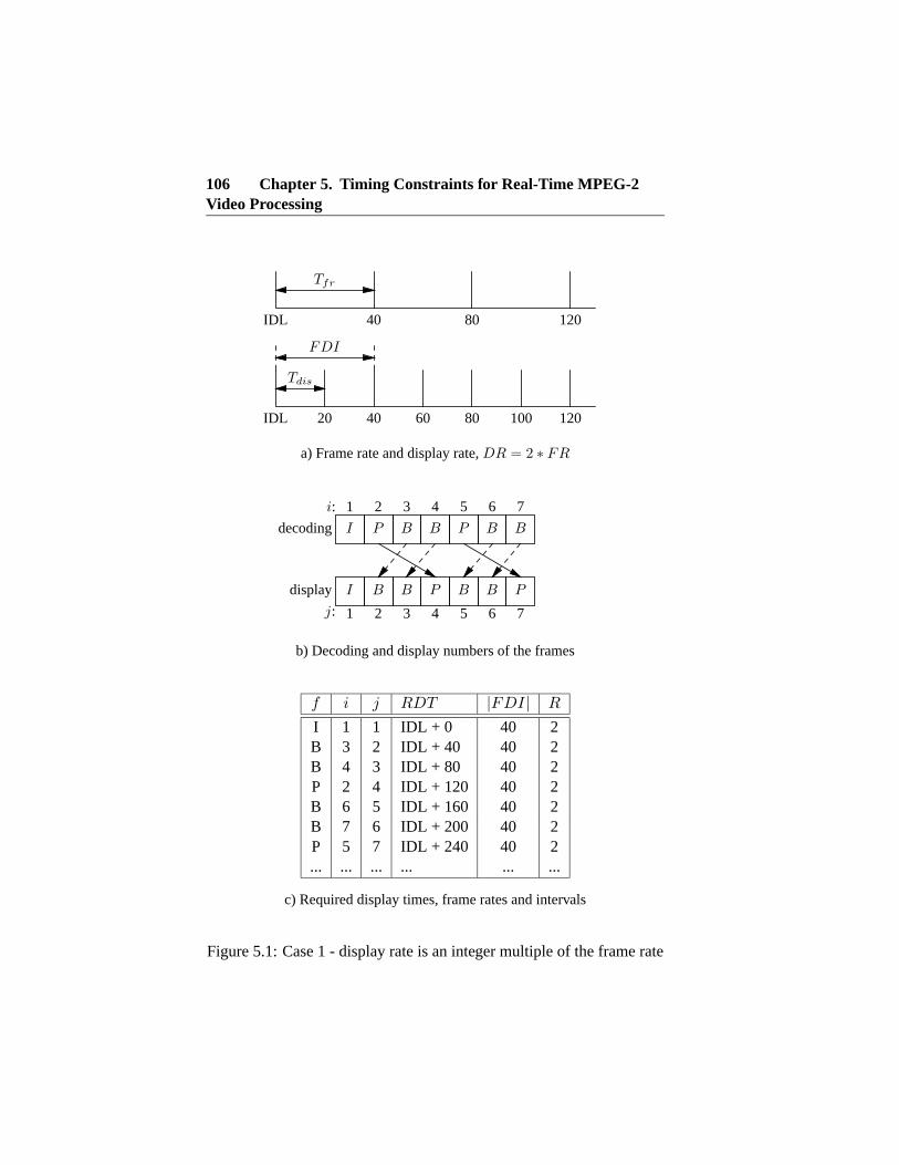
present a quality aware frame selection algorithm, to fully utilize limitedresources. Given that not all frames can be processed, it selects thosewhich will provide the best picture quality while matching the avail-able resources, starting only such decoding, which is guaranteed to becompleted.
As a final result, we provide a real-time method for flexible schedul-ing of media processing in resource constrained system. Results froma study based on realistic MPEG-2 video underline the effectiveness ofour approach.
We start by giving a general description of real-time systems andMPEG standard, followed by introduction to the two research areas andfinally their interaction.
1.1 Real-Time Systems Background
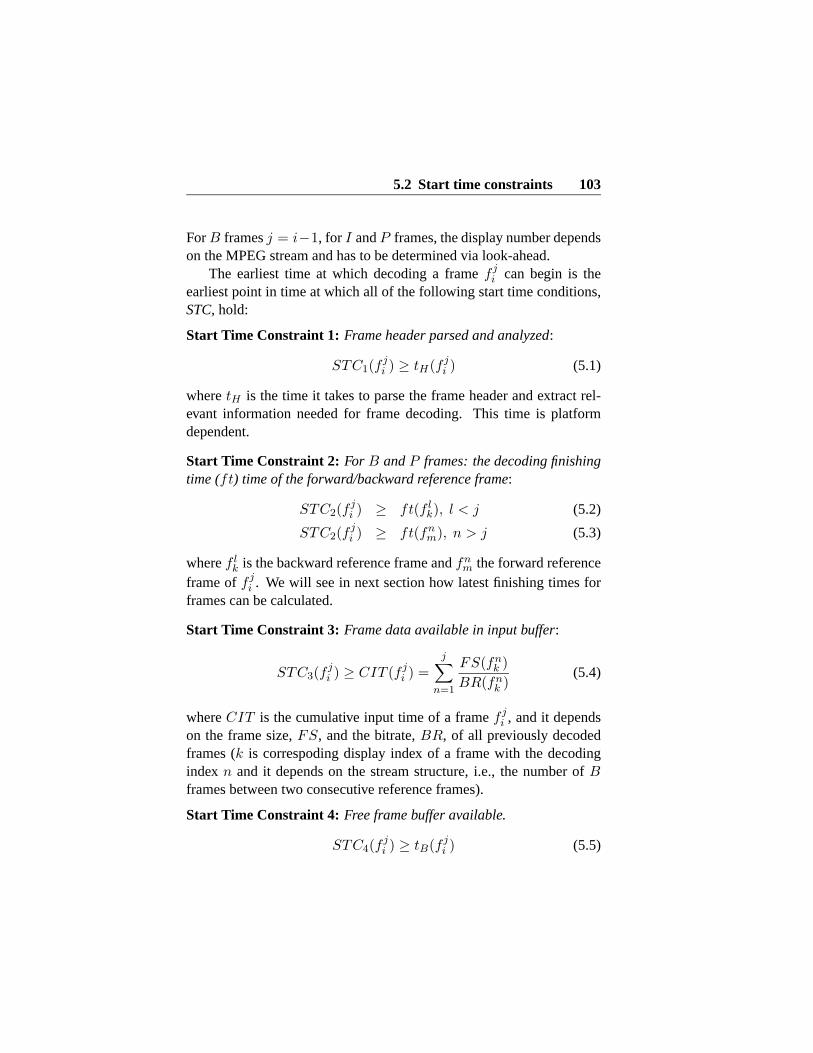
Real-time systems are computing systems in which meeting timing con-straints is essential to correctness. Usually, real-time systems are used tocontrol or interact with a physical system, where timing constraints areimposed by the environment. As a consequence, the correct behaviourof these systems depends not only on the result of the computation butalso at which time the results are produced [55]. If the system deliversthe correct answer after a certain deadline, it can be regarded as havingfailed.
Many applications are inherently of real-time nature; examples in-clude aircraft and car control systems, chemical plants, automated fac-tories, medical intensive care devices and numerous others. Most ofthese systems interact directly or indirectly with electronic and mechan-ical devices. Sensors provide information to the system about the stateof its external environment. For example, medical monitoring devices,such as ECG, use sensors to monitor patient status. Air speed, attitudeand altitude sensors provide aircraft information for proper execution offlight control plans etc.
Design of real-time systems must make sure that the system reactson external events in a timely way. The reaction may be a simple state
6 Chapter 1. Introduction
change, such as switching from red to green light, or a complicatedcontrol loop controlling many actuators simultaneously.
Real-time systems can be constructed out of sequential programs,but are typically built of concurrent programs, called tasks. A typicaltiming constraint on a real-time task is the deadline, i.e., the maximumtime interval within which the task must complete its execution. De-pending on the consequences that may occur due to a missed deadline,real-time systems are distinguished into two classes, hard and soft.
In hard real-time systems all task deadlines must be met, while insoft real-time systems the deadlines are desirable but not necessary. Inhard real-time systems, late data is bad data. Soft real-time systems areconstrained only by average time constraints, e.g., handling input datafrom the keyboard. In these systems, late data is still good data. Manysystems consist of both hard and soft real-time subsystems, and fromnow on we will refer to them as mixed real-time systems.
1.1.1 Real-time scheduling
When a processor has to execute a set of concurrent tasks, the CPU hasto be assigned to the various tasks according to a predefined criterion,called a scheduling policy. There is a great variety of algorithms pro-posed for scheduling of real-time systems today. Here we give a briefintroduction to some most common classifications, which have beenadopted in our research.
Offline vs online
Real-time scheduling algorithms fall into two categories [26]: offlineand online scheduling.
In offline scheduling, the scheduler has complete knowledge of thetask set and its constraints, such as deadlines, computation times, prece-dence constraints, etc. Scheduling decisions are based on fixed param-eters, assigned to tasks before their activation. The offline guaranteedschedule is stored and dispatched later during runtime of the system. Of-fline scheduling is also referred as static or pre-runtime or table-driven
1.1 Real-Time Systems Background 7
scheduling.On the other hand, online scheduling algorithms make their schedul-
ing decisions at run-time. All active tasks are reordered every time anew task enters the system or a new event occurs. Online schedulers areflexible and adaptive, but they can incur significant overheads becauseof run-time processing. Besides, online scheduling algorithms do notneed to have the complete knowledge of the task set or its timing con-straints. For example, an external event that arrives at the runtime ofthe system: we need to deal with it upon its arrival. Scheduling deci-sions are based on dynamic parameters that may change during systemevolution. Online scheduling is often referred to as dynamic or runtimescheduling.
Event-trigged vs time-trigged
There are two fundamentally different principles of how to control theactivity of a real-time system, event-trigged and time-trigged.
In event-trigged systems all activities are carried out in response torelevant events external to the system. When a significant event in theoutside world happens, it is detected by some sensor, which then causesthe attached device (CPU) to get an interrupt. For soft real-time sys-tems with lots of computing power to spare, this approach is simple,and works well. A problem with event-trigged systems is that they canfail under conditions of heavy load, i.e., when many events are happen-ing at once. As an example of an event-trigged system we can mentionthe SPRING system [52], which applies an online guarantee algorithmwith complex task models in distributed environments.
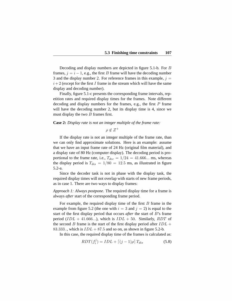
In a time-trigged system, all activities are carried out at certain pointsin time known a priori. Accordingly, all nodes in time-trigged systemshave a common notion of time, based on approximately synchronizedclocks. One of the most important advantages of time-trigged controlare predictable temporal behaviour of the system, which eases systemvalidation and verification considerably. An example of a time-triggedsystem is the MARS system [20].
In summary, event-triggered designs give faster response at low load
8 Chapter 1. Introduction
but more overhead and chance of failure at high load. This approach ismost suitable for dynamic environments, where dynamic activities canarrive at any time. Time triggered systems have the opposite propertiesand are suitable in relatively static environment in which a great deal isknown about the system behaviour in advance.
We will show in this work how event-triggered methods can be com-bined with time-triggered systems to provide for efficient inclusion ofdynamic activities, in particular sporadic ones.
Resource sufficient vs resource constrained
Scheduling can be further divided into scheduling algorithms that workin resource sufficient and those that work into resource constrained en-vironments [53], i.e., in overload situations.
A real-time system with enough resources is a system in which wealways can guarantee that all functions in the system will be able to per-form in time, i.e., before their deadlines. In these systems, the CPU willnever get overloaded, since those systems are designed for the worst-case scenario (peak load). In resource sufficient environments, eventhough tasks arrive dynamically, at any given time all tasks are schedu-lable. Examples include ABS brake systems, flight control systems, etc.,i.e., safety-critical systems.
On the other hand, in resource constrained systems, there will beoccasions when we cannot guarantee that all functions will make it intime. One example is a telephone switch system which is designed forthe average case load. In most of the cases the telephone switch systemworks well: when we call somebody, we usually get the dial tone rightaway, but when we try to dial on the New Year’s Eve, when all otherpeople try to call at the same time, the system might not be able toconnect our call (or we need to wait for some time).
Preemptive vs non-preemptive
Preemption is an operation of the kernel that interrupts the currentlyexecuting task and assigns the processor to a more urgent task ready to
1.1 Real-Time Systems Background 9
execute. Both offline and online scheduling can be either preemptive ornon-preemptive. Preemption increases the schedulability of the systemwhile non-preemtion gives an automatic mutual exclusion for access ofshared resources. Most of the scheduling algorithms are preemptive.
Heuristic vs optimal
An scheduling algorithm is said to be optimal if it minimizes some givencost function defined over the task set. On the other hand, if an algorithmtends toward but does not guarantee to find the optimal schedule is saidto be heuristic.
1.1.2 System model
Real-time systems span a large part of computer industry. So far most ofthe real-time systems research has been mostly confined to single nodesystems and mainly for single-processor scheduling. This needs to beextended for multiple resources and distributed nodes. In our work, weconsider a distributed system, i.e., one that consist of several processingand communication nodes [54]. We assume a discrete time model [40].Time ticks are counted globally, by a synchronized clock with granular-ity of slot length. Slots have uniform length and start and end at thesame time for all nodes in the system. Task periods and deadlines mustbe multiples of the slot length.
1.1.3 Task model
Real-time systems react on events that can be predictable (e.g., samplingof pulses generated by a pulse generator) or unpredictable (e.g., inter-rupts). Obviously, we need different task models for different types ofevents. There are three major types for real-time tasks:
Periodic Tasks
There are several definitions of periodic tasks. The most common one,that has also been adopted in our work, is that a periodic task consist of
10 Chapter 1. Introduction
an infinite sequence of identical activities, called instances, that are in-voked within regular time periods. Periodic tasks are commonly foundin applications such as avionics and process control where accurate con-trol requires continual sampling and processing data. We also refer toperiodic tasks as static, which indicates their exclusive treatment by theoffline scheduler.
Aperiodic Tasks
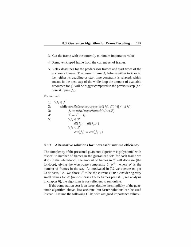
A type of task that consist of a sequence of identical instances, activatedat irregular intervals. Events that triggers an aperiodic task may occurat any time, e.g., a device generates interrupts, an operator presses theemergency button, alarms, etc. In general, aperiodic tasks are viewed asbeing activated randomly.
Furthermore, aperiodic tasks can be hard, soft and firm. Hard aperi-odic tasks have stringent timing constraint that must be met, while softaperiodic do not have deadlines at all. A firm aperiodic task has a dead-line that must be met once the task is guaranteed online. The differencebetween firm and hard aperiodic tasks is that hard tasks are guaranteedoffline, while firm tasks are guaranteed online, upon their arrival. Theycan also be rejected by the guarantee algorithm used.
Sporadic Tasks
Sporadic tasks [45] are introduced to model external events, such as aemergency button being pushed or a train crossing a sensor. However,the interval between successive events is imposed by the environment,i.e., events arrive at the system at arbitrary points in time, but with de-fined maximum frequency. They are invoked repeatedly with a (non-zero) lower bound on the duration between consecutive occurrences ofthe same event. Therefore, each sporadic task will be invoked repeat-edly with a lower bound on the interval between consecutive invocationsi.e., minimum inter-arrival time between two consecutive invocations.
In other words, a sporadic task is a dynamic type of task charac-terized by a minimum inter-arrival time (mint) between consecutive in-
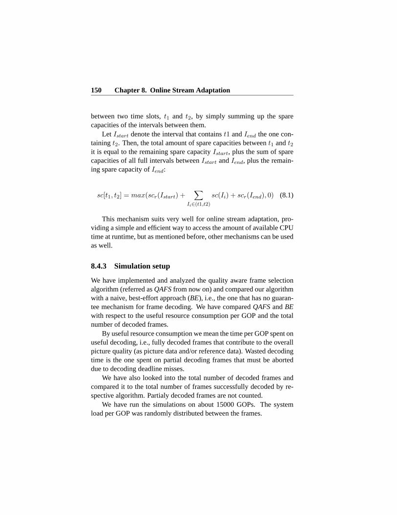
1.1 Real-Time Systems Background 11
stances. After the minimum inter-arrival time has elapsed, the next in-stance can get activated at any time – we do not know when.
In the study of mixed real-time systems, it is a common model thatperiodic tasks are hard and therefore deterministic, while aperiodic tasksare soft or firm. Sporadic tasks, on the other hand, provide enoughknowledge to assess their timing. They can therefore be required tobe hard.
1.1.4 Simple and complex constraints
We distinguish between simple constraints, i.e., period, start-time, anddeadline, for the earliest deadline first scheduling model [23], and com-plex constraints. We refer to such relations or attributes of tasks as com-plex constraints, which cannot be expressed directly in the earliest dead-line first scheduling model using period, start-time, and deadline. Inmost of the cases, offline transformations are needed to schedule theseat runtime (some can be resolved online at the cost of the higher over-head). Here are some examples of complex constraints:
• Synchronization – Execution sequences, such as sampling - com-puting - actuating require a precedence order of task execution.
• Jitter – The execution start or end of certain tasks, e.g., samplingor actuating in control systems, is constrained by maximum vari-ations.
• Non-periodic execution – Non-periodic constraints, such as someforms of jitter, require instances of tasks to be separated by nonconstant length intervals. Similar reasoning applies to constraintsover more than one instance of a task, e.g., for iterations, datahistory or ages. A constraint can be of the type “separate theexecution of instance i and i + 4 by no more than max and noless than min”.
12 Chapter 1. Introduction
• Non-temporal constraints – Demands for reliability, performance,or other system parameters impose demands on tasks from a sys-tem perspective, e.g., to not allocate two tasks to the same node,or, e.g., to have minimum separation times, etc.
• Application specific constraints – Applications may have demandsspecific to their nature. Duplicated messages on a bus in an au-tomotive environment, for example, may need to follow a cer-tain pattern due to interferences such as EMI. Wiring can havelength limitations, imposing allocation of certain tasks to nodesaccording to their geographical positions. An engineer may wantto improve schedules, creating constraints reflecting his practicalexperience.
1.2 Overview of PART I: Efficient Scheduling ofMixed Task Sets with Complex Constraints
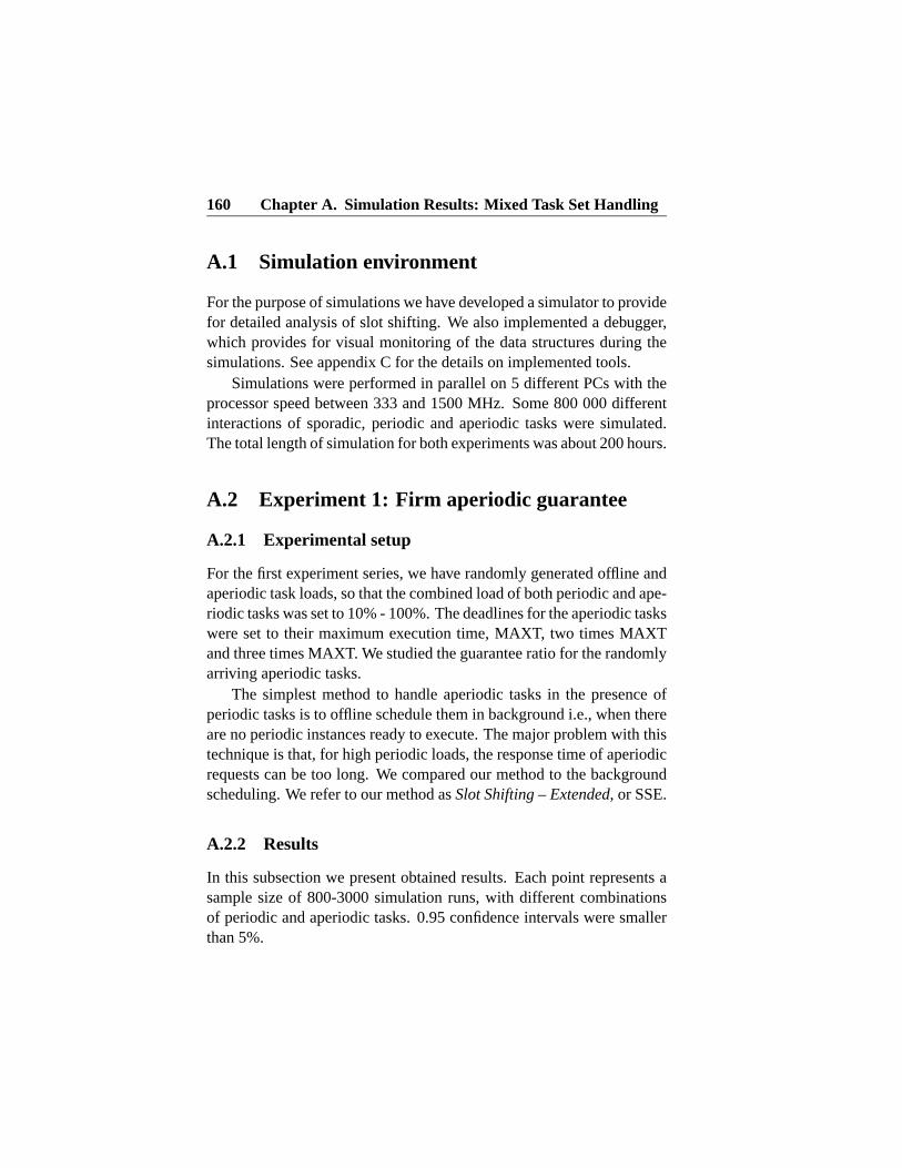
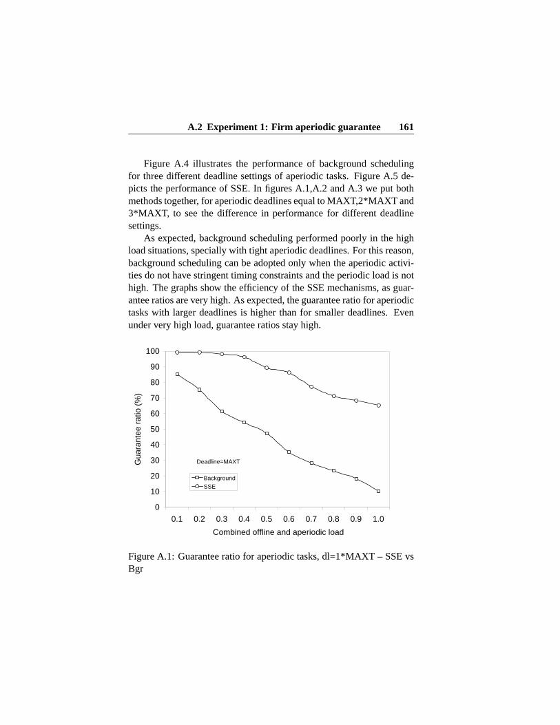
The design of safety-critical real-time systems has to put focus on de-mands for predictability, flexibility, and reliability. If we have an ap-plication with completely known characteristics, we can achieve pre-dictable behaviour of the system, e.g., linear and angular position sen-sors that read a robot’s arm position every 20 ms and adjust it via steppermotors. On the other hand, many external events are not predictable, forexample, an external stimulus such as pressing a button. Systems mustreact to these sporadic events when they occur rather than when it mightbe convenient. By taking care of them we introduce flexibility to thesystems.
As a first part of this thesis, we provide mechanisms to handle un-predictable, dynamic events together with predictable ones. We presenta combined offline and online approach to deal with a combination ofmixed sets of tasks and constraints: periodic tasks with complex andsimple constraints, soft and firm aperiodic tasks, and in particular spo-radic tasks.
1.2 Overview of PART I: Efficient Scheduling of Mixed Task Setswith Complex Constraints 13
1.2.1 Related work
A variety of algorithms have been presented to handle periodic and dy-namically arriving tasks. Here we restrict ourselves to work most sig-nificant for our own work.
Aperiodic task handling
One common method to handle aperiodic task is the server-based ap-proach. Dynamic arrivals are given access to the resources reserved fora so called server task. If an aperiodic task arrives it executes with theresources of the server task. If no dynamic task is demanding execution,the server task will not execute.
Handling of firm aperiodic requests using a Total Bandwidth Serverhas been presented in [51]. Online guarantees of aperiodic tasks in firmperiodic environments, where tasks can skip some instances, have beendescribed in [16].
The Deferrable Server [42] algorithm is a method to improve theaverage response times of aperiodic tasks with respect to polling service.
Sporadic server [50] algorithm allows to enhance the average re-sponse time of aperiodic tasks without degrading the utilization boundof periodic tasks. It aims at the shortest response time in the presence ofhard real time periodic tasks executing on a fixed priority basis.
Example algorithms for the selection of tasks to reject in overloadsituations have been discussed in [14], [41], [7], [3]. These algorithmsassume control over all tasks in the system and do not take into accountthe impact of offline scheduled tasks.
Sporadic task handling
There are two major techniques to handle sporadic tasks. One is toassume maximum arrival frequency and fit them in the periodic frame-work. The other one is to always be prepared for their unknown arrivaltimes by performing an offline schedulability test for their worst-casearrival scenario.
14 Chapter 1. Introduction
In [45] sporadic tasks are fitted into the periodic framework by trans-forming them into pseudo-periodic tasks. A set of rules are applied toderive the deadline and period of a sporadic task to fulfill the requiredtiming.
An online algorithm for scheduling sporadic tasks with shared re-sources in hard real-time systems has been presented in [38]. Schedul-ing of sporadic requests with periodic tasks on an earliest-deadline-first(EDF) basis has been presented in [59].
A schedulability test for sporadic tasks on single processors has beenpresented in [8]. Necessary and sufficient conditions are derived for asporadic task set to be feasible.
An offline guarantee algorithm for sporadic tasks based on band-width reservation has been presented in [15] for single processor sys-tems.
Complex timing constraints handling
An algorithm for the transformation of precedence constraints on sin-gle processor to suit the EDF scheduling model has been presented in[19]. However, many industrial applications require allocation of taskswith precedence constraints on different nodes, i.e., a distributed systemwith internode communication. The transformation of precedence con-straints with an end-to-end deadline in this case requires subtask dead-line assignment to create execution windows on the individual nodes sothat precedence is fulfilled, e.g., [24].
A schedulability analysis for pairs of tasks communicating via a net-work instead of decomposition has been presented in [60].
In [68] static scheduling is discussed as a general technique for solv-ing the problem of satisfying complex timing constraints in hard real-time systems. The conclusion is that pre-run-time scheduling is essen-tial to meeting such constraints in large systems.
The application of standard timing constraints, such as deadlinesand periods, can sometimes overconstrain specifications. One way toovercome this is to use dynamic timing constraints with a feasibilityfunction describing temporal requirements instead of providing concrete
1.2 Overview of PART I: Efficient Scheduling of Mixed Task Setswith Complex Constraints 15
constraints such as periods and deadlines. A method that shows how dy-namic timing constraints can be used instead with standard schedulingalgorithms has been presented in [30].
Combined offline and online scheduling
The slot shifting algorithm to combine offline and online schedulingwas presented in [28]. It focuses on inserting aperiodic tasks into of-fline schedules by modifying the runtime representation of available re-sources. The use of information about the amount and distribution ofunused resources for non-periodic activities is similar to the basic ideaof slack stealing [58], [21] which applies to fixed priority scheduling.Slot shifting does not provide for easy removal of guaranteed tasks. Be-sides, while appropriate for including sequences of aperiodic tasks, theoverhead for sporadic task handling becomes too high.
A similar approach for combined offline and online scheduling hasbeen recently proposed in [65, 64, 63]. It creates a generalized offlinepre-schedule for a set of time-trigged tasks, with some slack left foreventual event-driven workload competing for resources. The differ-ence between this method and the slot shifting is that slot shifting doesa reactive approach, i.e., taking an existing offline schedule and try-ing to accommodate aperiodic and sporadic tasks, while pre-schedulingapproach is proactive, i.e., it makes a schedule that can fit the aperiod-ics and sporadics later on. Besides, this approach is aimed for singleprocessor and independent tasks, whereas slot shifting can be used indistributed real-time systems, with inter-node communication and notindependent tasks.
1.2.2 Motivation
The methods for handling dynamic tasks described above can generallybe classified as latest start time methods, since they all share the charac-teristic of postponing the execution of hard tasks in order to give moreresources to the soft tasks. Normally, as long as all guaranteed tasks
16 Chapter 1. Introduction
meet their deadlines, it does not matter if they complete their executionin advance of their deadline or just before it.
However, these methods concentrate most on particular types ofconstraints. As mentioned before, a real-time system might need to ful-fill some complex constraints, in addition to basic temporal constraintsof tasks, such as periods, start-times and deadlines. Those complex con-straints can not be expressed as generally as the simple ones. Addingcomplex constraints to a chosen scheduling strategy increases schedul-ing overhead [69] or requires new, specific schedulability tests whichmay have to be developed.
Constraints such as some forms of jitter, e.g., for feedback loop de-lay in control systems [61], require instances of tasks to be separatedby non-constant length intervals. In order to fit these constraints intothe periodic task model, it can easily happen that we end up with anover-constrained specification. At the same time, algorithms are com-putationally expensive [6].
Besides, most of the existing methods for handling sporadic tasksperform only an online acceptance test, which introduces extra overheadto the system. When a set of sporadic tasks arrives at runtime, a sched-uler performs an acceptance test. The test succeeds if each sporadic taskin the set can be scheduled to meet its deadline, without causing anypreviously guaranteed tasks to miss its deadline, else it is rejected. Adisadvantage with this approach is that if the set has been rejected, it istoo late for countermeasures.
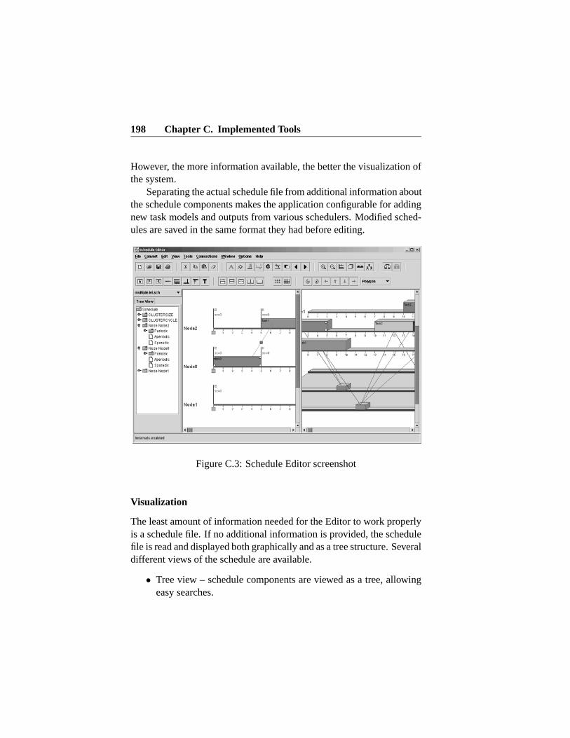
1.2.3 Approach
Dynamically arriving tasks cannot be fitted into a fixed periodic frame-work, i.e., their handling has to be prepared explicitly for unknown oc-currence times. Offline schedules will generally not be tight, i.e., therewill be times where resources are unused. In this work we try to ef-ficiently reclaim those resources, and use it for dynamic arrivals, i.e.,aperiodic and sporadic tasks.
Our method provides an offline schedulability test for sporadic tasks,based on slot shifting [28]. It constructs a worst case scenario for the ar-
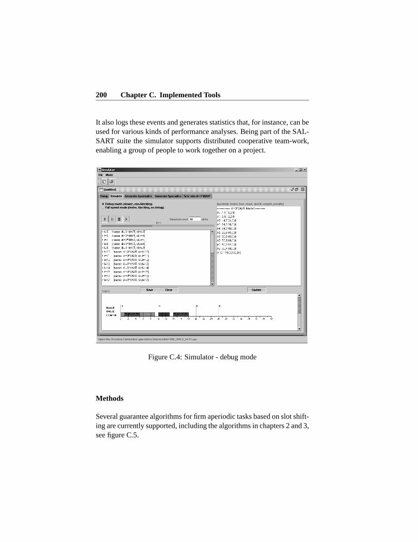
1.2 Overview of PART I: Efficient Scheduling of Mixed Task Setswith Complex Constraints 17
rival of the sporadic task set and tries to guarantee it on the top of the of-fline schedule. The guarantee algorithm is applied at selected slots only.At runtime, it uses the slot shifting mechanisms to feasibly schedulesporadic tasks in union with the offline scheduled periodic tasks, whileallowing resources to be reclaimed for aperiodic tasks. Since the majorpart of preparations is performed offline, the involved online mecha-nisms are simple. Furthermore, the reuse of resources allows for highresource utilization.
As a final result of this work, we provide algorithms to deal witha combination of mixed sets of tasks and constraints: periodic taskswith complex and simple constraints, soft and firm aperiodic, and inparticular sporadic tasks. Instead of providing algorithms tailored for aspecific set of constraints, we propose an EDF based runtime algorithm,and the use of an offline scheduler for complexity reduction to transformcomplex constraints into the EDF model. At runtime, an extension toEDF, two level EDF, ensures feasible execution of tasks with complexconstraints in the presence of additional tasks or overloads.
Combined offline and online Scheduling
Offline scheduling methods can accommodate many specific constraintsbut at the expense of runtime flexibility, in particular inability to handledynamic activities such as aperiodic and sporadic tasks. Consequently, adesigner given an application composed of mixed tasks and constraintshas to choose which constraints to focus on in the selection of schedul-ing algorithm; others have to be accommodated as well as possible. Ifwe only use online scheduling, then we might introduce high overheadfor resolving complex constraints, or, in the worst case, we cannot re-solve them at all.
Our method is a combined offline and online approach: it integratesoffline, time-trigged scheduling and dynamic, event-trigged scheduling.We use slot shifting to eliminate all types of complex constraints be-fore the runtime of the system. They are transformed into a simpleEDF model, i.e., periodic tasks with start times and deadlines. Dynamicactivities, i.e., aperiodic and sporadic tasks, are incorporated into of-
18 Chapter 1. Introduction
fline schedule by making use of the unused resources and leeways in theschedule.
We assume a resource restricted environment, where dynamic ac-tivities have to be guaranteed to fit into the offline schedule, withoutaffecting any of previously scheduled or guaranteed activities. We pro-vide both offline and online mechanisms for dealing with such a prioriunknown activities.
The method requires a small runtime data structure, simple run-time mechanisms, going through a list with increments and decrements,provides O(N) acceptance tests, N being the number of aperiodic in-stances, and facilitates changes in the set of tasks, for example to handleoverloads. Furthermore, our method provides for handling of slack ofnon-periodic tasks as well, e.g., instances of tasks can be separated byintervals other than periods.
Handling aperiodic tasks
The methods presented in this thesis provide for inclusion of both firmand soft aperiodic tasks. Firm tasks must be guaranteed while the softones do not require any acceptance test.
Upon arrival of a firm aperiodic task, a test determines whether thereare enough resources available to include it feasibly in the set of previ-ously guaranteed tasks and if the scheduling strategy will ensure timelycompletion. If the task can be accepted, it is guaranteed by providing amechanism which ensures that the resources it requires will be availablefor its execution.
Handling sporadic tasks
Offline scheduling is not suitable for handling sporadic tasks due to un-known arrival times. One approach could be to transform sporadic tasksinto equivalent pseudo-periodic tasks [45] offline, which can be sched-uled simply at runtime. However, this may lead to significant under-utilization of the processor time, especially when the deadline of thepseudo-periodic task is small compared to the minimum inter-arrival
1.2 Overview of PART I: Efficient Scheduling of Mixed Task Setswith Complex Constraints 19
time of the sporadic task. That because a great amount of time has tobe reserved offline, before the runtime of the system, for servicing dy-namic request from sporadic tasks. In extreme cases, a task handling anevent which is rare, but has a tight deadline, may require reservation ofall resources.
We present a combined offline and online approach for handlingsporadic tasks. The offline transformation determines resource usageand distribution as well, which we use to handle sporadic tasks. Offlinewe assume the worst case scenario for arrival patterns for sporadic tasks,and online we try to reduce this pessimism by using the current infor-mation about the system. Dynamic activities are accommodated withoutaffecting the feasible execution of statically scheduled tasks.
1.2.4 Contribution summary
We present methods to schedule sets of mixed types of tasks with com-plex constraints, by using earliest deadline first scheduling and offlinecomplexity reduction. In particular, we proposed an algorithm to handlesporadic tasks to improve response times and acceptance of firm aperi-odic tasks.
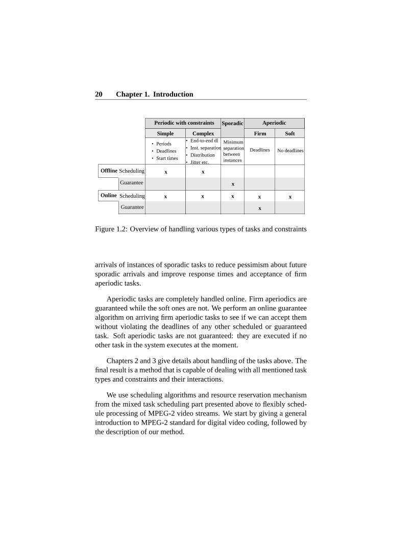
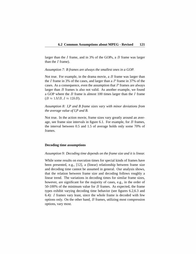
Our methods use a general technique, capable of incorporating var-ious types of constraints and their combinations. Those are resolvedin the offline part of the method, without degrading the system perfor-mance at runtime. Table 1.2 gives an overview of when different typesof tasks are handled by our method (simple periodic and complex peri-odic in the table refer to periodic tasks with simple respective complexconstraints).
Periodic tasks are completely handled offline. Complex constraintsare translated into simple ones, i.e., only start times and deadlines andthe tasks are scheduled to execute before their deadline. Originally, thetasks are scheduled to execute as soon as possible, but they may also beshifted online within their feasibility intervals in order to accept moreaperiodic or sporadic tasks.
Sporadic tasks are guaranteed offline for the worst-case arrival pat-terns and scheduled online, where an online algorithm keeps track of
20 Chapter 1. Introduction
• Periods• Deadlines• Start times
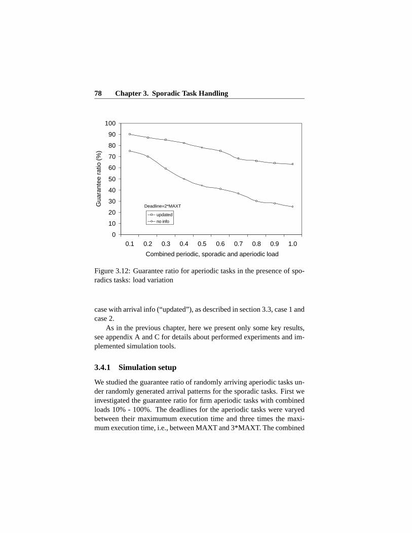
SchedulingOffline
Deadlines
Aperiodic
No deadlines
Firm Soft
Sporadic
Minimumseparationbetweeninstances
Periodic with constraints
• End-to-end dl• Inst. separation• Distribution• Jitter etc.
Simple Complex
x
x
x
x
x
x x
x
x
Guarantee
Online
Guarantee
Scheduling
Figure 1.2: Overview of handling various types of tasks and constraints
arrivals of instances of sporadic tasks to reduce pessimism about futuresporadic arrivals and improve response times and acceptance of firmaperiodic tasks.
Aperiodic tasks are completely handled online. Firm aperiodics areguaranteed while the soft ones are not. We perform an online guaranteealgorithm on arriving firm aperiodic tasks to see if we can accept themwithout violating the deadlines of any other scheduled or guaranteedtask. Soft aperiodic tasks are not guaranteed: they are executed if noother task in the system executes at the moment.
Chapters 2 and 3 give details about handling of the tasks above. Thefinal result is a method that is capable of dealing with all mentioned tasktypes and constraints and their interactions.
We use scheduling algorithms and resource reservation mechanismfrom the mixed task scheduling part presented above to flexibly sched-ule processing of MPEG-2 video streams. We start by giving a generalintroduction to MPEG-2 standard for digital video coding, followed bythe description of our method.
1.3 MPEG-2 Background 21
1.3 MPEG-2 Background
The Moving Picture Experts Group (MPEG) standard for coded repre-sentation of digital audio and video [1] is used in a wide range of ap-plications. MPEG is one of the most popular audio/video digital com-pression technique because it is not just a single standard. Instead, itis a range of standards suitable for different applications but based onsimilar principles.
MPEG group defines several standards in digital video, among it theMPEG-1 standard, used e.g., in Video CDs, the MPEG-2 standard, usede.g., in DVDs, digital video broadcasting, high-definition TVs (HDTV),and the MPEG-4 standard, used e.g., in picture phones, streaming me-dia, Internet. It also defines several audio standards – among them MP3and AAC.
MPEG-2 is currently the most used video standard of the MPEGgroup. In particular, MPEG-2 has become the coding standard for digi-tal video streams in consumer content and devices, such as DVD moviesand digital television set top boxes for Digital Video Broadcasting (DVB).
It should be noted that MPEG is a standard for the format, a syntax,not for the actual encoding. The specification only defines the bit streamsyntax and decoding process. Generally, this means that any decoderswhich conform to the specification should produce near identical outputpictures. However, decoders may differ in how they respond to errorsintroduced in the transmission channel. For example, an advanced de-coder might attempt to conceal faults in the decoded picture if it detectserrors in the bit stream. As a consequence, the same content, e.g., amovie, can be encoded in many ways while adhering to the same stan-dard. In fact, MPEG encoding has to meet diverse demands, depending,e.g., on the medium of distribution, such as overall size in the case ofDVD, maximum bit rate for DVB, or speed of encoding for live broad-casts.
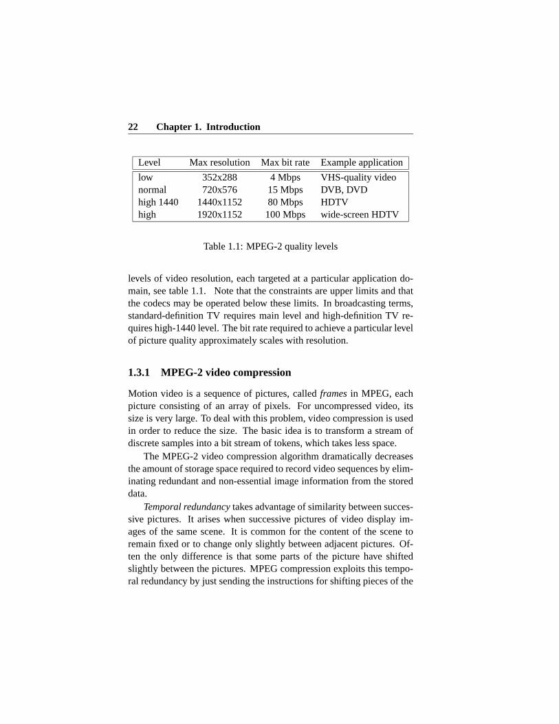
In this thesis we deal with MPEG-2, which is currently the mostused MPEG standard. It aims to be a generic video coding system sup-porting a diverse range of applications. The standard covers four quality
22 Chapter 1. Introduction
Level Max resolution Max bit rate Example application
levels of video resolution, each targeted at a particular application do-main, see table 1.1. Note that the constraints are upper limits and thatthe codecs may be operated below these limits. In broadcasting terms,standard-definition TV requires main level and high-definition TV re-quires high-1440 level. The bit rate required to achieve a particular levelof picture quality approximately scales with resolution.
1.3.1 MPEG-2 video compression
Motion video is a sequence of pictures, called frames in MPEG, eachpicture consisting of an array of pixels. For uncompressed video, itssize is very large. To deal with this problem, video compression is usedin order to reduce the size. The basic idea is to transform a stream ofdiscrete samples into a bit stream of tokens, which takes less space.
The MPEG-2 video compression algorithm dramatically decreasesthe amount of storage space required to record video sequences by elim-inating redundant and non-essential image information from the storeddata.
Temporal redundancy takes advantage of similarity between succes-sive pictures. It arises when successive pictures of video display im-ages of the same scene. It is common for the content of the scene toremain fixed or to change only slightly between adjacent pictures. Of-ten the only difference is that some parts of the picture have shiftedslightly between the pictures. MPEG compression exploits this tempo-ral redundancy by just sending the instructions for shifting pieces of the
1.3 MPEG-2 Background 23
previous picture to their new positions in the current picture. The cod-ing technique that exploit temporal redundancy is called Inter-coding(inter=between).
Spatial redundancy takes advantage of similarity among most neigh-boring pixels within the same picture. It occurs because parts of the pic-ture are often replicated (with minor changes) within a single picture.For example, regions of sky or walls are almost entirely the same color.If several pixels point in the same area, MPEG compression exploitsthis spatial redundancy by sending the color for whole region just once,instead of sending it for each pixel. The coding technique that exploitspatial redundancy is called Intra-coding (intra=within).
Another way to archive higher compression ratios is amplitude scal-ing, i.e., the reduction of the color depth of each pixel in a picture andcolor space scaling, i.e., the number of colors available for displayingan image is reduced.
Furthermore, an MPEG-2 video stream can be coded with constantor variable bit rate. Constant bit rate, CBR, means that the rate at whichthe video data should be consumed is constant. It varies the quality levelof the video frames in order to ensure a consistent bit rate throughout anencoded file. Variable bit rate, VBR, varies the amount of output datain each time segment based on the complexity of the input data in thatsegment. The goal is to maintain constant quality instead of maintaininga constant data rate by making intelligent bit-allocation decisions duringthe encoding process. CBR is useful for streaming multimedia contenton limited capacity channels since CBR would make usage all of theavailable capacity. VBR is preferred for storage because it makes betteruse of storage space: more space is allocated to more complex segmentswhile less space is allocated to less complex segments.
1.3.2 MPEG-2 stream organization
The output of a single video or audio encoder is known as elementarystream. MPEG standard defines ways of multiplexing more than oneelementary stream (video, audio and data) into one single system stream.In MPEG-2 there are two different types of system streams, transport
24 Chapter 1. Introduction
stream and program stream.The program stream is used for combining together elementary streams
that have a common time base and need to be displayed in a synchro-nized way. Such streams are suited for transmission in a relatively error-free environment and enable easy software processing of the receiveddata. Program Stream packets may be of variable and relatively greatlength. This form of multiplexing is used for video playback and forsome network applications. DVD uses Program Streams.
The transport stream is used for multiplexing streams that do not usea common time base. The transport streams packets have fixed length of188 bytes. Transport streams are suited for transmission in which theremay be potential packet loss or corruption by noise, or/and where thereis a need to send more than one program at a time. Digital broadcastinguses Transport Streams.
In this thesis we deal with MPEG-2 Elementary Video Streams. Weuse real-time methods to adjust video streams in overload situations.
1.4 Overview of PART II: Real-Time Processingof MPEG-2 Video in Resource Constrained Sys-tems
The MPEG-2 standard is predominant in consumer electronics for DVDplayers, digital satellite receivers, and TVs today. One common thingfor all devices is that the encoded content has to be decoded and playedout. Decoding can be performed in hardware or in software, or in a mixof both. Both dedicated and programmable decoders can be based onaverage-case requirements if they provide means to gracefully handleoverload situations. If not, both must support worst-case requirements.
Within the next few years, MPEG-2 decoding will move from ded-icated hardware to software, for reasons of cost, rapid upgradeability,and configurability. In a software implementation, it is possible to usethe slack on the processor for other applications in average case. Withdedicated hardware, there are no such possibilities. As a consequence,
1.4 Overview of PART II: Real-Time Processing of MPEG-2 Videoin Resource Constrained Systems 25
the behavior of a software decoder will be less regular than that of adedicated hardware decoder. Coping with these irregularities is one ofthe objectives dealt with in this thesis.
Furthermore, video will not only be watched on classic TV sets, butincreasingly displayed on smaller devices ranging from mobile phonesto web pads, providing mobility. Consequently, MPEG-2 decoding willbe performed in software under limited resources.
Most current software decoders, however, operate under the assump-tion of sufficient resources, using buffering and rate adjustment based onaverage-case assumptions. These provide acceptable quality for appli-cations such as video transmissions over the Internet, when decreasesin quality, delays, uneven motion or changes in speed are tolerable. Inhigh quality consumer terminals, however, quality losses of such meth-ods are not acceptable. In fact, producers of such devices have arguedto mandate the use of hard real-time methods instead [10].
In this thesis, we present methods for quality aware MPEG-2 videostream adaptation under limited resources, based on realistic timing con-straints for MPEG-2 decoding.
1.4.1 Related work
Here is an overview of related work relevant to ours.
Real-time multimedia processing
The Constant Bandwidth Server (CBS) algorithm for integrating multi-media and hard real-time tasks has been presented in [2]. It providesreal-time guarantees for hard real-time tasks and probabilistic guaran-tees for soft multimedia tasks. Hard tasks are guaranteed based onworst-case execution time and minimum interarrival times, while CBSis used for soft multimedia tasks. Each multimedia task is assigned amaximum bandwidth, calculated using the average execution time anddesired activation time. If a task needs more bandwidth, it may slowdown, but still not jeopardize hard tasks. Our work shows that the aver-age assumptions will not hold for a significant number of cases.
26 Chapter 1. Introduction
A method for real-time scheduling and admission control of MPEG-2 video streams that fits the need for adaptive CPU scheduling has beenpresented in [25]. The method qualifies for continuous re-processingand guarantees quality of service. However, it requires separate decod-ing tasks for different frame types. We found this to be an unnecessaryrestriction: one decoding task can be used for all frame types. Besides,frame skipping decisions are made based on frame type only. As a con-sequence, stream quality might be degraded more than neccessary.
An approach that allows close-to-average-case resource allocationto a single video processing task has been proposed in [67]. It is basedon asynchronous, scalable processing, and QoS adaptation. No frametype distinction has been made and the method applies only on a specialcase when the display rate of the display device is equal to the framerate of the movie. We solve this problem for the general case, where thedisplay rates are different from the frame rates.
A method to process multimedia in fixed-priority based systems hasbeen presented in [11]. Resource allocation for media processing isachieved by using periodic budgets provided by a budget scheduler. Themethod introduces notion of conditionaly guaranteed budgets as a wayto handle structural overloads. The idea is to assign budgets to multime-dia applications and if an application is not using its budget, it is given toanother application. The method requires extensions to existing budgetscheduler and online budget management.
A frame skipping pattern based on QoS-human has been presentedin [46]. QoS-human is a measurement of video quality from a humanperception, i.e., a group of people watch movies with different numberof skipped frames and write down their perception of the video quality.Then, the user perception is mapped to the number of skipped frames todetermine different values of QoS-human. However, only one skippingcriterion, QoS human, has been applied when selecting frames, takingno consideration about frame sizes, buffer and latency requirements, orcompression methods used.
Quality reduction for MPEG decoding and other video algorithmsis discussed in [48], [70], [32], and [39]. The decoder reduces the load
1.4 Overview of PART II: Real-Time Processing of MPEG-2 Videoin Resource Constrained Systems 27
by using a downgraded decoding algorithm. This approach requires al-gorithms that can be downgraded, with sufficient quality levels to allowsmooth degradation. Such algorithms are not yet widely available.
Worst-case execution times for multimedia tasks
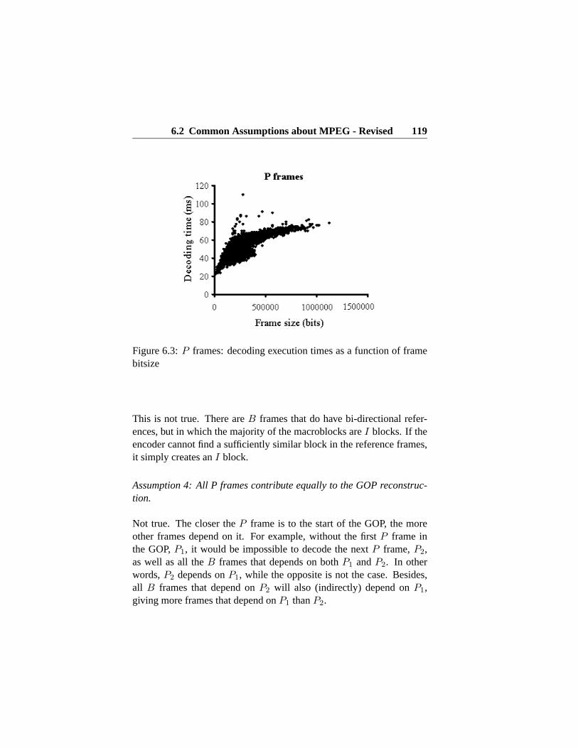
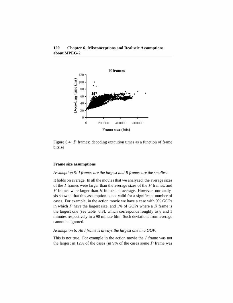
It is difficult to predict WCET for decoding parts. MPEG-2 can use dif-ferent bit rates which can result in large differences in decoding timesfor different streams. This could lead to big overestimations of theWCETs. Work on predicting MPEG execution times has been presentedin [9, 12]. It assumes a linear relationship between frame size and de-coding, which we show not to be the case in general.
The design and implementation of a software decoder for MPEGvideo bit streams is described in [44]. It shows how MPEG video couldbe decoded in real-time using a software-only implementation on desk-top computers. Worst-case execution times for the different parts of thedecoding process are reported. Frame prediction from reference framesis found to be most computationally expensive. We relate to this find-ings when making frame skipping decisions if the processing power islimited.
1.4.2 Motivation
MPEG-2 encoding has to meet diverse demands, depending, e.g., on themedium of distribution, such as overall size in the case of DVD, maxi-mum bit rate for DVB, or encoding speed for live broadcasts. In the caseof DVD and DVB, sophisticated provisions to apply spatial and tempo-ral compression are applied, while a very simple, but quickly codedstream will be used for the live broadcast. Consequently, video streams,and in particular their decoding demands will vary greatly between dif-ferent media.
Most standard decoders fail to satisfy the demands of MPEG-2 inoverload situations as they do not consider the specifics of this com-pression standard. In resource limited situations the processor cannot
28 Chapter 1. Introduction
work fast enough to decode all the frames, the workload for the soft-ware decoder has to be reduced. One way to achieve this is skip someof the frames.
Naive best-effort decoders perform frame skipping by simply run-ning out of time at frame display time, incurring either a sudden distur-bance in smoothness, as pictures are missing, or a delay of subsequentframes, disturbing motion speed. As frame decoding starts and pro-ceeds without knowing about timely completion, it may happen that theresources are fully used, but wasted, as partially decoded video framesare generally not useful. In extreme cases, the decoding of a large andimportant frame might just not make it, therefore being lost and imped-ing quality, while simply skipping to decode a small preceding framemight have freed the resources for completion, with only slight qualityreduction.
In addition, skipping a frame may affect also other frames due tointer frame dependencies. In a typical movie, a single frame skip canruin around 0.5 seconds of motion video. Thus frame skipping needsappropriate assumptions and constraints about streams to be effective.
1.4.3 Approach
In this thesis we present a method for quality aware MPEG-2 streamadaptation in resource constrained systems. The method provides bestquality by selecting frames if not all can be decoded under limited re-sources. It is based on a priority ordering for frame skipping takingframe importance for the overall video quality into account. It cre-ates ensembles of decoding tasks for the video frames, each with tim-ing constraints suited specifically for the particular frame, transformingthe video stream into such tailored for actual demand and available re-sources.
Using a real-time system for resource management, the frame selec-tion algorithm takes into account the actual state of the system, by deter-mining the best frames utilizing the available resources and consideringthe priority ordering for skipping. Thus, our algorithm selects framesbased on concrete frame knowledge and ensures that only decoding of
1.4 Overview of PART II: Real-Time Processing of MPEG-2 Videoin Resource Constrained Systems 29
frames which can be completed in time is started.Below is the overview of the steps used in our method. Each of them
will be described in details in separate chapters of this thesis.
MPEG-2 processing under limited resources
As a initial step in our work, we have studied MPEG-2 standard in de-tails and looked into the requirements for timely processing of MPEG-2 video streams. We identified the stream requirements, as well as thebuffer and latency requirements that need to be fulfilled for smooth play-out. Furthermore, we outlined possible methods for stream adaptationwhen the system resources are not enough to process entire stream.
Timing constrains for MPEG-2 decoding
Video stream processing has real-time deadlines in a sense missing adecoding deadline of an important frame can result in significant visualartifact. Based on the requirements above, we present actual demandsfor MPEG-2 playout and derive timing constraints for frame decoding.We show that standard, fixed timing constraints are restrictive and flexi-ble ones are better suited for MPEG-2 software decoding.
Analysis of MPEG-2 streams
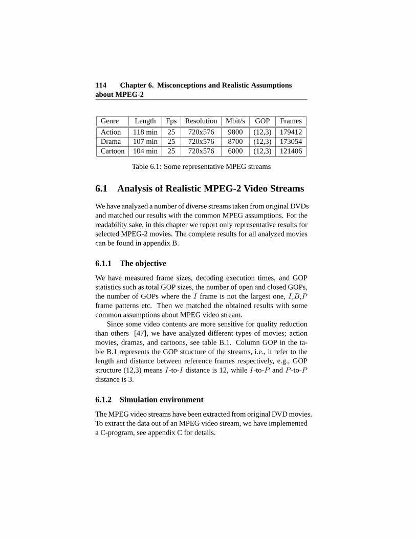
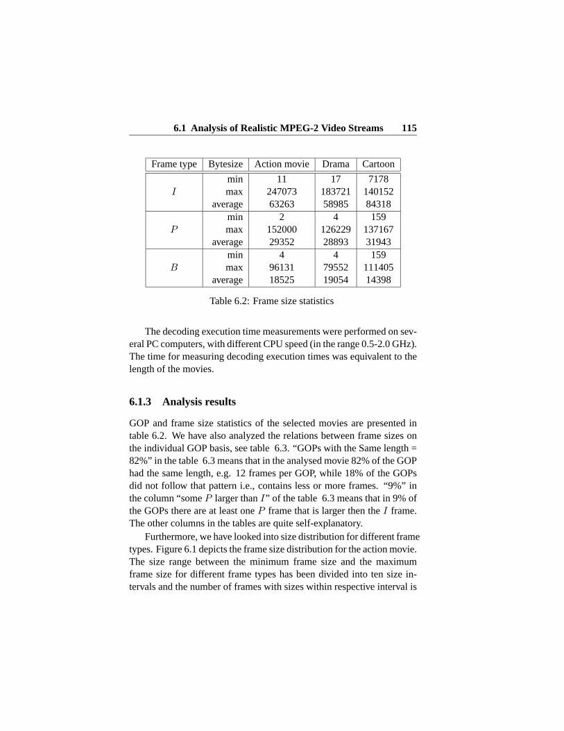
As the next step towards a method for flexible processing of mediastream, we have performed a proper analysis of diverse MPEG-2 videostreams to identify realistic assumptions about MPEG-2. We have matchedthe results with common assumptions about MPEG, and found a numberof misconceptions present in the literature.
Criteria for frame skipping
Frame skipping needs appropriate assumptions to be effective. Drop-ping the wrong frame at the wrong time can result in a noticeable distur-bance in the played video stream. Here we use the realistic assumptions
30 Chapter 1. Introduction
from our MPEG-2 analysis to propose a set of criteria for frame skip-ping.
Frame selection algorithm
Based on identified frame skipping criteria, we present an algorithm forquality aware frame selection when it is not possible to decode all framesin time. We apply the proposed criteria on a set of frames and assigndifferent importance values to the frames. These will be used to makedecision which frames are to be skipped first in overload situations.
Online stream adaptation
Here we unite the frame selection algorithm, decoding timing constraintsand real-time resource management from our work on mixed task setshandline to provide a method for for quality aware MPEG-2 streamadaptation in resource constrained systems. The algorithm provides bestvideo quality by selecting frames if not all can be decoded under limitedresources.
While the frame selection algorithm is independent of the actual guar-antee algorithm used, making it suitable to work with a variety of algo-rithms and paradigms, we present its use with a concrete scheduler – theone that we used to schedule mixed sets of task in the first part of thethesis.
1.4.4 Contribution summary
Here is a summary of contributions from our work on MPEG-2 videostream processing. We have:
• identified requirements for real-time MPEG-2 processing
• identified misconceptions about MPEG-2
• proposed realistic assumptions for MPEG-2
1.5 Relation between Contributions in PART I and PART II 31
• proposed criteria for frame skipping
• derived timing constraints for MPEG-2 decoding
• showed how MPEG-2 streams can flexibly be scheduled underlimited resources
We present a method for quality aware MPEG-2 stream adaptationunder limited resources, based on realistic timing constraints for MPEGdecoding. As an example, we show how we can adjust streams in thecontext of our previous work, i.e., combined offline and online schedul-ing. Simulation study underlines the effectiveness of our approach.
1.5 Relation between Contributions in PART I andPART II
In the first part of the thesis we show how we can flexibly schedulemixed sets of tasks, i.e., periodic, aperiodic and sporadic, with simpleand complex constraints by using integrated offline and online approachbased on the slot shifting method [28].
In the second part, we present a method for flexible processing ofmedia streams under limited resources. Here we need a mechanism toaccess the available system resources in order to know how to adapt avideo stream, i.e., how many frames can be timely decoded. We alsoneed a real-time scheduler to schedule processing of the stream.
We use the scheduling mechanism and the resource reservation mech-anism from the first part of the thesis to flexibly schedule MPEG-2 videostreams. As a final result of the thesis, we provide a real-time method forflexible scheduling of media processing in resource constrained system.
1.6 Outline of the thesis
The rest of this thesis is organized as follows:
32 Chapter 1. Introduction
Chapter 2 describes handling of soft and firm aperiodic task togetherwith offline scheduled tasks. It starts by giving an overview of the origi-nal slot shifting method for joint online and offline scheduling, followedby the new method for handling firm aperiodic tasks.
Chapter 3 presents a method to handle sporadic tasks by guarantee-ing them offline for the worst-case, and reducing this pessimism onlineby keeping track on sporadic arrivals. As a final result, we present amethod to schedule mixed sets of tasks with simple and complex con-straints.
Chapter 4 gives an overview of MPEG-2 video streams and sets upreal-time model for their processing. Latency and buffer requirementsare discussed. This chapter gives a basis for the remaining work onMPEG in this thesis.
Chapter 5 uses results and finding about MPEG-2 processing andrequirements from chapter 4 to derive realistic timing constraints forMPEG-2 video decoding.
Chapter 6 presents an exhaustive analysis of MPEG-2 video streams,identifies a number of misconceptions about MPEG-2 and proposes re-alistic assumptions about MPEG-2 processing.
Chapter 7 identifies valid criteria for frame skipping, based on as-sumptions from previous chapter, and proposes an algorithm for qualityaware frame selection when it is not possible to decode all frames intime.
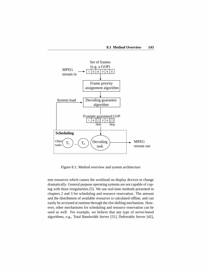
Chapter 8 presents a final method for quality aware MPEG-2 streamadaptation. It combines the two research parts by using the schedul-ing mechanisms from the first part to flexible schedule processing ofMPEG-2 video in resource limited systems.
Chapter 9 concludes the thesis and outlines possible application ar-eas and future work.
A significant amount of our work and results has been moved to sev-eral appendixes for readability reasons:
Appendix A presents all simulation results for scheduling of mixedtasks sets. It gives details about the simulation setup, performed experi-
1.6 Outline of the thesis 33
ments and confidence intervals.Appendix B contains analysis setup and results for diverse realistic
MPEG-2 video streams.Appendix C gives an overview of all tools used for obtaining results
in this thesis. Both own implemented tools and tools done by otherpeople but used by us are described here.
– PART I –
Efficient Scheduling of Mixed Task Sets withComplex Contraints
Chapter 2
Aperiodic Task Handling
A number of industrial applications advocate the use of time-triggeredapproaches for reasons of predictability, cost, product reuse, and mainte-nance. The rigid offline scheduling schemes used for time-triggered sys-tems, however, do not provide for flexibility. Offline scheduling meth-ods can resolve many specific constraints but at the expense of runtimeflexibility, in particular inability to handle dynamically arriving tasks,such as aperiodic and sporadic tasks. At runtime, aperiodic tasks thathandle asynchronous external events can only be included into the un-used resources of the offline schedule, supporting neither guarantees norfast response times.
In this chapter we present an algorithm for flexible handling of firmaperiodic tasks in offline scheduled systems. Aperiodic tasks that arriveat runtime, are guaranteed and incorporated into the offline schedule bymaking use of the unused resources and leeways in the schedule. Weuse the offline part of slot shifting [30], to eliminate all types of com-plex constraints before the runtime of the system. Then we propose anew online guarantee algorithm for dealing with dynamic tasks. Ouralgorithm provides an O(N) complexity acceptance test, where N isthe number of aperiodic tasks, to determine if a set of aperiodics can befeasibly included into the offline scheduled tasks, and does not requireruntime handling of resource reservation for guaranteed tasks. Thus, it
37
38 Chapter 2. Aperiodic Task Handling
supports flexible schemes for rejection and removal of aperiodic tasks,overload handling, and simple reclaiming of resources. As a result, ouralgorithm [34] provides for a combination of offline scheduling and on-line firm aperiodic task handling.
We start by presenting the basic idea for aperiodic task handling insection 2.1, followed by the description of the original slot shifting ap-proach, section 2.2. In section 2.3, we present our new online algorithmfor flexible aperiodic task handling. We compare the original slot shift-ing approach for aperiodic handling with the new method in section 2.4followed by the simulation results, section 2.5 and the chapter summaryin section 2.6.
2.1 Basic Idea for Aperiodic Task Guarantee
Guaranteeing and handling of firm aperiodic tasks involves three steps:
Acceptance test
Upon arrival of a firm aperiodic task, a test determines whether thereare enough resources available to include it feasibly in the set of previ-ously guaranteed tasks and if the scheduling strategy will ensure timelycompletion.
Reservation of resources
If the task can be accepted, it is guaranteed by providing a mechanismwhich ensures that the resources it requires will be available for its ex-ecution. This can be achieved, e.g., by removing these resources fromthe available ones, or by ensuring that subsequent guarantees will notremove them. Note that acceptance test and guarantee can be separated.
Rejection strategy
A failed acceptance test indicates an overload situation. The commonresponse, not to guarantee the task under consideration, assumes that
2.2 Slot Shifting - Original Approach 39
already guaranteed tasks are more important than newly arriving ones.This is, however, not generally the case. Rather, the importance order ofthe tasks is independent of their arrival time. Consequently, a rejectionstrategy is required, which determines which task or tasks – out of allguaranteed or newly arrived tasks – to reject or abort.
2.2 Slot Shifting - Original Approach
In this section, we briefly describe the slot shifting method [28] whichwe use as a basis to combine offline and online scheduling. It providesfor the efficient handling of aperiodic tasks on top of a table-driven,offline schedule with general task constraints. Slot shifting extracts in-formation about unused resources and leeway in an offline schedule anduses this information to add tasks feasibly, i.e., without violating re-quirements on the already scheduled tasks.
2.2.1 Offline preparations
First, a standard offline scheduler, e.g., [49], or [29] creates schedulingtables for the periodic tasks. The scheduling tables list fixed start-and end times of task executions, eliminating all flexibility. The onlyassignments fixed by the specification of the tasks’ feasibility, however,are the initiating and concluding tasks in the precedence graph, all othertasks may vary within the precedence order, i.e., they can be shifted.
After offline scheduling, and calculation of start-times and dead-lines, the schedule is divided into a set of disjoint execution intervalsfor each node. Spare capacities to represent the amount of availableresources are defined for these intervals.
Each deadline calculated for a task defines the end of an interval Ii.Several tasks with the same deadline constitute one interval. Note thatthese intervals differ from execution windows, i.e. start times and dead-line: execution windows can overlap, intervals with spare capacities, asdefined here, are disjoint. The deadline of an interval is identical to thedeadline of the task. The start, however, is defined as the maximum of
40 Chapter 2. Aperiodic Task Handling
the end of the previous interval or the earliest start time of the task. Theend of the previous interval may be later than the earliest start time, orearlier (empty interval). Thus it is possible that a task executes outsideits interval, i.e., earlier than the interval start, but not before its earlieststart time.
The spare capacities of an interval Ii are calculated as given in for-mula 2.1:
sc(Ii) = |Ii| −∑T∈Ii
wcet(T ) + min(sc(Ii+1), 0) (2.1)
The length of Ii, minus the sum of the activities assigned to it, is theamount of idle time in that interval. These have to be decreased by theamount “lent” to subsequent intervals: Tasks may execute in intervalsprior to the one they are assigned to. Then they “borrow” spare capac-ity from the “earlier” interval. See [28] for details on the borrowingmechanism of slot shifting.
2.2.2 Online mechanism
After determination of intervals and spare capacities, the offline prepa-rations are completed and the amount and location of unused resourcesis available for online use, i.e., for guaranteeing firm aperiodic tasks.The basic idea is to use two level EDF, i.e., to schedule tasks accordingto - “normal level”, but give priority -“priority level” to an offline taskwhen it needs to start at latest, similar to the basic idea of slack stealing[58] [21] for fixed priority scheduling. Thus, the CPU is not completelyavailable for runtime tasks, but reduced by the amount allocated for of-fline tasks. So, we need to know the amount and location of resourcesavailable after the offline tasks are guaranteed, which we calculate in theoffline part of slot shifting as described above.
During system operation, the on-line scheduler is invoked after eachslot. It checks whether aperiodic tasks have arrived, performs the guar-antee algorithm, and selects a task for execution. This decision is thenused to update the intervals and spare capacities. Finally the schedulingdecision is executed in the next slot.
2.2 Slot Shifting - Original Approach 41
Guarantee algorithm
Assume that an aperiodic task A with deadline dl(A) is tested for guar-antee at current time t. We identify three parts of the total spare capaci-ties available:
• sc(Ic)t, the remaining spare capacity of the current interval,
• ∑sc(Ii), c < i ≤ l, end(Il) ≤ dl(A) ∧ end(Il+1) > dl(A),
sc(Ii) > 0, the positive spare capacities of all full intervals be-tween t and dl(A), and
• min(sc(Il+1), dl(A)−start(Il+1)), the spare capacity of the lastinterval, or the execution need of A before its deadline in thisinterval, whichever is smaller.
If the sum of all three is larger than the worst-case execution time of A,then A can be accommodated, and therefore guaranteed.
Upon guarantee of a task, the spare capacities are updated to reflectthe decrease in available resources. Also, if dl(A) is not equal to the endof an interval, the interval in which dl(A) occurs must be split, resultingin a creation of a new interval.
Scheduling
If the spare capacities of the current interval sc(Ic) > 0, EDF is appliedon the set of ready tasks - “normal level”. sc(Ic) = 0 indicates that aguaranteed task has to be executed or else a deadline violation in thetask set will occur. It will execute immediately - “priority level”. Sincethe amount of time spent at priority level is known and represented inspare capacity, guarantee algorithms include this information.
In original slot shifting, after each scheduling decision, the sparecapacities of the affected intervals are updated. If, in the current in-terval Ic, an aperiodic task executes, or the CPU remains idle for oneslot, current spare capacity in Ic is decreased. If an offline task assignedto Ic executes spare capacity does not change. If an offline task T as-signed to a later interval Ij , j > c executes, the spare capacity of Ij is
42 Chapter 2. Aperiodic Task Handling
increased - T was supposed to execute there but does not, and that ofIc decreased. If Ij “borrowed” spare capacity, the “lending” interval(s)will be updated. The reader is referred to [27, 28] for details on slotshifting.
2.3 Slot Shifting - New approach
The runtime mechanisms of the original version of slot shifting addedtasks by modifying this data structure, creating new intervals, which isnot suitable for frequent changes as required by e.g., sporadic tasks. Ournew guarantee method separates acceptance and guarantee. It only mod-ifies spare capacity, without creating new intervals, which eliminates theonline modifications of intervals and spare capacities as in original slotshifting and, thus, allows rejection strategies over the entire aperiodictask set.
2.3.1 Basic idea
The basic idea behind the method is based on standard earliest deadlinefirst guarantee, but sets it to work on top of the offline schedule: EDFis based on having full availability of the CPU; we have to considerinterference from offline scheduled tasks and pertain their feasibility.
Assume, at time t1, we have a set of guaranteed aperiodic tasks Gt1
and an offline schedule represented by offline tasks, intervals, and sparecapacities. At time t2, t1 < t2 , a new aperiodic A arrives. Meanwhile,a number of tasks of Gt1 may have executed; the remanining task setat t2 is denoted Gt2 . We test if A ∪ Gt2 can be accepted, consideringoffline tasks. If so, we add A to the set of guaranteed aperiodics. Noexplicit reservation of resources is done, which would require changesin the intervals and spare capacities. Rather, resources are guaranteed byaccepting the task only if it can be accepted together with the previousguaranteed and offline scheduled ones. This enables the efficient use ofrejection strategies.
2.3 Slot Shifting - New approach 43
2.3.2 Algorithm description
Let Gt1 denote a set of guaranteed, not yet finished firm aperiodic tasksat time t1, ordered by increasing deadlines:
where n is the number of tasks in Gt1 , ct1(Gi) denotes the remainingexecution time of task Gi at time t1, and dl(Gi) is its absolute dead-line. We keep track of how much each task has executed, which meanswe know the remaining execution times of each task at any time. If aguaranteed task has not yet started to execute, the remaining executiontime is equal to its actual execution time, i.e., ct1(Gi) = c(Gi). Tasks inGt1 are ordered by increasing deadlines, meaning that task Gi has ear-lier deadline than task Gi+1. We also know that each task in Gt1 has adeadline later than t1.
Now assume a new firm aperiodic task A arrives at time t2, with theexecution time c(A) and absolute deadline dl(A). From time t1 to t2,some tasks in Gt1 could have executed up to t2, which is reflected asfollows:
• {G1, ..., Gk−1} are the tasks completed by t2:
{∀Gi ∈ Gt1 | ct2(Gi) = 0, 1 ≤ i ≤ k − 1}
where ct2(Gi) denotes the remaining execution time of task Gi attime t2.
• Gk is the current task, according to EDF. It may have executedpartially before t2, so we need only to consider its remaining ex-ecution time, ct2(Gk) ≤ c(Gk).
• {Gk+1, ..., Gn} are not yet started tasks that need to execute fully:
{∀Gi ∈ Gt1 | ct2(Gi) = c(Gi), k + 1 ≤ i ≤ n}
44 Chapter 2. Aperiodic Task Handling
So, when guaranteeing a new aperiodic task A at time t2, we need notconsider already completed tasks, but only the remaining portion of thecurrent task and the tasks that have not started yet:
Gt2 ⊂ Gt1 , Gt2 = {Gk, Gk+1, ...Gn}
A new aperiodic task A is accepted if the set G′ = Gt2 ∪ A is feasible,considering the offline scheduled and guaranteed tasks.
2.3.3 Acceptance test for aperiodic tasks
Spare capacities and intervals of slot shifting make sure that all of-fline scheduled tasks are guaranteed to complete before their deadlines.Those offline tasks are scheduled to execute as late as possible, but underrun-time they can be executed earlier, i.e., we can shift their executionwithin their feasibility window.
Aperiodic tasks utilize unused resources in the offline schedule. Theamount and location of available resources are represented as intervalsand spare capacities. So, we want to insert aperiodic tasks without vio-lating the feasibility of offline tasks.
Let A = {A1, A2, ..., An} be a set of firm aperiodic tasks that needto be scheduled together with the offline tasks. We accept the aperiodicset if each task in A is guaranteed to complete before its deadline, i.e.,the following must hold:
∀i, 1 ≤ i ≤ n : c(Ai) ≤{
sc[t, dl(A1)] , i = 1sc[ft(Ai−1), dl(Ai)] , i > 1
where t is current time and notation sc[t1, t2] means the spare capacityfrom time t1 to time t2. Otherwise, we need to reject some task(s).
Note that the spare capacities are not distributed in a uniform waythroughout the schedule. Rather, as described in 2.2, the schedule isdivided into intervals, each with an individual value of spare capacity.Consequently, the amount of spare capacity in a window depends on theposition of that window in the schedule.
2.3 Slot Shifting - New approach 45
The finishing time of a firm aperiodic task Ai is calculated withrespect to the finishing time of the previous task, Ai−1. Without anyoffline tasks, it is calculated the same as in EDF algorithm:
ft(Ai) = ft(Ai−1) + c(Ai)
Since we guarantee firm aperiodic tasks on a top of an offline schedule,we need to consider the feasibility of offline tasks. This extends theformula above with a new term that reflects the amount of resourcesreserved for offline tasks:
ft(Ai) = c(Ai) +
{t + R[t, ft(A1)] , i = 1ft(Ai−1) + R[ft(Ai−1), ft(Ai)] , i > 1
where R[t1, t2] stands for the amount of resources (in slots) reserved forthe execution of offline tasks from time t1 to time t2. We can accessR[t1, t2] via spare capacities and intervals at runtime:
R[t1, t2] = (t2 − t1) − max(sc[t1, t2], 0)
As ft(Ai) appears on both sides of the equation, a simple solution is notpossible. Rather, we present an algorithm for computation of finishingtimes of firm aperiodic tasks with complexity of O(N), which is furtherdiscussed in next subsection.
2.3.4 Algorithm description
We now present the acceptance test for a firm aperiodic tsk A and algo-rithm for finishing time calculation in pseudo code.
Step 1: Let Gt denote the set of previously guaranteed aperiodic tasksat time t, with sorted deadlines, as described in subsection 2.3.2 above.Find the position of the last task, Gi, in the set Gt, that has deadlinebefore the currently guranteed task A, i.e., the place in Gt where A willbe inserted:
for(i = 1; dl(Gi) < dl(A); i + +);
46 Chapter 2. Aperiodic Task Handling
Step 2: Get the finishing time of A based on the finishing time of itspredecessor Gi, and A’s execution demand. The start point for calcu-lation of the finishing time is either the current time t or the finishingtime of A’s predecessor, whichever is later (see below for details ongetFinishingTime(..) function).
ft = getF inishingT ime(max(ft(Gi), t), c(A));
Step 3: If A can be finished before its deadline, then go through allthe tasks in Gt with deadlines after dl(A) and for each task calculate itsnew finishing time, with respect to the new task A (execution of all taskswith the deadline later by A will be delayed by A). New finishing timesare then compared to the tasks’ deadlines. If any of the investigatedtasks fails to complete before its deadline, that means that adding A toGt would result in a set that is not feasible, i.e., not all tasks in Gt willcomplete before their deadlines. We can either reject A or some othertask(s) in Gt. Otherwise, if all tasks can be finished by their deadlineseven if A added, then insert A into the set of previously guaranteed firmaperiodic tasks Gt.
if(ft ≤ dl(A)){
/* check if accepting A will cause any of the previously/* guaranteed firm aperiodic tasks to miss its deadline*/for(j = i + 1; j < n; j + +){
ft = getFT (ft, ct(Gj));if(ft> dl(Gj)){
/* not feasible! */reject = true;break;
}}
2.3 Slot Shifting - New approach 47
if(!reject)insert(A,Gt);
else/* apply some rejection startegy */
}else reject A
Function: getFinishingTime() calculates the finishing time of a taskbased on predecessor task’s finishing time, ftp, and the remaining ex-ecution demand, cr, of the task to investigate. First, it calculates theremaining spare capacity, scr, of the current interval, Ik, i.e., the inter-val that contains the finishing time of the previous task, ftp, which isthe earliest possible start time for the current task. Without offline tasks,finishing time is equal to the finishing time of the predecessor task in-creased by the computation demand of the current task. In the presenceof offline tasks, however, we do not have all CPU time available, butonly the spare capacities in intervals. Hence, we need to go through allthe intervals between the starting point ftp until execution demand isexhausted, i.e., we “simulate” the execution of the investigated task bygoing through intervals and “filling up free slots”, until the remainingexecution time is exhausted. The function returns the calculated finish-ing time of the current task.
getF inishingT ime(ftp, cr){
/* get current interval */Ik = getInterval(ftp);
/* get remaining spare capacity of the current interval */scr = start(Ik) + sc(Ik) − ftp;
/* go through the intervals and ”fill up” free slotsuntil the remaining execution demand is exhaused */
48 Chapter 2. Aperiodic Task Handling
while(cr > scr){if(scr (Ik) > 0)
cr = cr − scr;k + +;ftp = start(Ik)scr = sc(Ik);
}return (ftp + cr);
}
2.3.5 Complexity
The complexity of our algorithm is O(N), N being the number of firmaperiodic tasks to be guaranteed, because we go through all tasks onlyonce, and calculate their finishing times on the way, as depicted in figure2.1. The for-loop picks a task and start the while-loop, which calculatesits finishing time by going through the intervals. Then we pick anothertask, and continue traversing the intervals at the point where we gotinterrupted by for-loop, and so on. We do not have any nested loops,and we always continue forward.
fti fti+1 fti+2 fti+3
Ik Ik+1 Ik+2 Ik+3
while while while
Ai+1 Ai+2 Ai+3 Ai+4for
Figure 2.1: Online acceptance test for firm aperiodic tasks – algorithmcomplexity
2.3 Slot Shifting - New approach 49
2.3.6 Example
Assume an offline schedule with intervals and spare capacities as de-picted in figure 2.2 (the shaded boxes represent offline tasks). Let G3 be
0 1 2 3 4 5 6 7 8 9 10 11 12 13 14 15 16 17 18 19
I1,sc=3 I2,sc=2 I3,sc=2 I4,sc=3
Figure 2.2: Example online firm aperiodic guarantee– static schedule
the set of previously guaranteed but not completed firm aperiodic tasksat current time t = 3:
G3 = {G1(3, 10), G2(2, 18), G3(1, 19)}where the first parameter is the remaining execution time, the secondabsolute deadline. Tasks is G3 are ordered by increasing deadlines. Attime t = 3 we have the execution scenario of both offline scheduledtasks and guaranteed aperiodic tasks from G3 as described in figure 2.3.Guaranteed firm aperiodic tasks will execute in the first available slots,in EDF order.
0 1 2 3 4 5 6 7 8 9 10 11 12 13 14 15 16 17 18 19
I1 I2 I3 I4
G1 G1G2 G2G3
Figure 2.3: Example online firm aperiodic guarantee – execution with-out new task.
Now assume a firm aperiodic task A(4, 16) arrives at run-time att = 3. We perform the online guarantee algorithm to investigate if wecan accept A:
1. Task G1 has earlier deadline than A, so G1’s position in the set G3
remains unchanged, i.e., before A. We do not need to guarantee itagain.
50 Chapter 2. Aperiodic Task Handling
0 1 2 3 4 5 6 7 8 9 10 11 12 13 14 15 16 17 18 19
I1 I2 I3 I4
G1 G1
2. Task G2 has a deadline after the deadline of A, which meansthat the A should execute before G2. We must check if there areenough resources available for A to complete before its deadline.We calculate the finishing time of A which is slot 15:
ftA = getFT (ftG1 , c(A)) = 15 < 16
The finishing time is less than the deadline of A, which meansthat A could complete in time.
0 1 2 3 4 5 6 7 8 9 10 11 12 13 14 15 16 17 18 19
I1 I2 I3 I4
G1 G1 A A A
3. Now we must check if accepting task A will cause any of otherguaranteed firm aperiodic tasks (G2, G3) to miss their deadlines.We calculate their finishing times:
Both G2 and G3 can complete before their deadlines, which meansthat the new task A can be guaranteed and therefore inserted in theset of guaranteed firm aperiodic tasks G3.
0 1 2 3 4 5 6 7 8 9 10 11 12 13 14 15 16 17 18 19
I1 I2 I3 I4
G1 G1 A A A G2 G3
2.4 Improvements over original slot shifting 51
2.4 Improvements over original slot shifting
Here are the improvements over the original slot shifting acceptance testfor a set of firm aperiodic tasks:
Implicit resource reservation
The method presented here reserves resources implicitly, by only ac-cepting a new task if it can be guaranteed together with all previouslyguaranteed ones, and does not require runtime handling of resourcereservation for guaranteed tasks, as the original slot shifting. Conse-quently, removal of guaranteed tasks and changes in the set of tasks canbe handled efficiently.
Flexible rejection strategies
Our method allows for easy changes in the set of guaranteed tasks andthus supports flexible rejection strategies. It allows a new set of candi-dates to be submitted to the acceptance test and does not require modi-fications to the reserved resources for guaranteed tasks. In original slotshifting, if a firm aperiodic task cannot be feasibly included into the ex-isting schedule, then the task is rejected. In our approach, we can choseto reject any of the guaranteed but not yet finished firm aperiodic tasks,and keep the currently guaranteed tasks instead.
Efficient resource reclaiming
Should aperiodic tasks use less resources than expressed in worst caseparameters, our method directly reclaims these without recalculation ofavailable resources. The next time the acceptance test is performed, thefact that a task has an earlier finishing time is considered in the calcu-lations by simply starting the calculation of the finishing point of thecurrently guaranteed task earlier, i.e., we start to ”fill up” remaining ex-ecution time for the currently guaranteed task at an earlier point in time.
52 Chapter 2. Aperiodic Task Handling
This also results in an earlier finishing time of the current task, leavingmore space for other executions.
Improved overload handling
Overload handling schemes can easily be applied, since our method pro-vide a set of firm aperiodic tasks from which any of the tasks can berejected. One such overload handling method based on our algorithmhas been presented in [17]. Even other overload handling schemes, suchas presented in [14] and [3] can be used.
2.5 Simulation Analysis
We have implemented the algorithms for firm aperiodic tasks describedabove and have run simulations for various scenarios. We have studiedthe guarantee ratio for aperiodic tasks for different combinations of totalsystem loads and aperiodic deadlines.
For the purpose of simulations we have developed a simulator toprovide for detailed analysis of slot shifting. We also implemented adebugger, which provides for visual monitoring of the data structuresduring the simulations.
Here we present some key results, see appendix A for details aboutthe simulation setup, performed experiments and confidence intervals.Also see appendix C for the information about the tools that we imple-mented for the simulation purpose.
2.5.1 Simulation setup
We have randomly generated offline and aperiodic task loads, so thatthe combined load of both periodic and aperiodic tasks was set between10% and 100%. The deadlines for the aperiodic tasks were set to theirmaximum execution time, MAXT, two times MAXT and three timesMAXT. We studied the guarantee ratio for the randomly arriving aperi-odic tasks.
2.5 Simulation Analysis 53
Method: Background
0
10
20
30
40
50
60
70
80
90
100
0.1 0.2 0.3 0.4 0.5 0.6 0.7 0.8 0.9 1.0
Combined offline and aperiodic load
Gua
rant
ee r
atio
(%
)
deadline=3*MAXTdeadline=2*MAXTdeadline=1*MAXT
Figure 2.4: Guarantee ratio for aperiodic tasks – Background scheduling
The simplest method to handle aperiodic tasks in the presence ofperiodic tasks is to offline schedule them in background i.e., when thereare no periodic instances ready to execute. The major problem with thistechnique is that, for high periodic loads, the response time of aperiodicrequests can be too long. We compared our method to the backgroundscheduling. We refer to our method as Slot Shifting – Extended, or SSE.
2.5.2 Results
Figure 2.4 illustrates the performance of background scheduling forthree different deadline settings of aperiodic tasks, while figure 2.5 de-picts the performance of the extended slot shifting approach. Each pointin the graphs represents a sample size of 800-3000 simulation runs, withdifferent combinations of periodic and aperiodic tasks. 0.95 confidence
54 Chapter 2. Aperiodic Task Handling
intervals were smaller than 5%.
Method: SSE
0
10
20
30
40
50
60
70
80
90
100
0.1 0.2 0.3 0.4 0.5 0.6 0.7 0.8 0.9 1.0
Combined offline and aperiodic load
Gua
rant
ee r
atio
(%
)
deadline=3*MAXTdeadline=2*MAXTdeadline=1*MAXT
Figure 2.5: Guarantee ratio for aperiodic tasks – SSE (our approach)
As expected, background scheduling performed poorly in the highload situations, especially with tight aperiodic deadlines. For this rea-son, background scheduling can be adopted only when the aperiodicactivities do not have stringent timing constraints and the periodic loadis not high.
The graphs show the effectiveness of the SSE mechanisms, as guar-antee ratios are very high. As expected, the guarantee ratio for aperiodictasks with larger deadlines is higher than for smaller deadlines. Evenunder very high load, guarantee ratios stay high.
2.6 Chapter summary 55
2.6 Chapter summary
In this chapter we presented an algorithm for flexible handling of firmaperiodic tasks in offline scheduled systems. It is based on slot shifting,a method to combine offline and online scheduling methods.
First, a standard offline scheduler constructs a schedule, resolvingcomplex task constraints such as precedence, distribution, and end-to-end deadlines. Then, the offline schedule is analyzed for unused re-sources, i.e., intervals and spare capacities are calculated. Offline sched-uled task can flexibly execute within their corresponding intervals. It isalso possible for an offline task to executes outside its interval, i.e., ear-lier than the interval start, but not before its earliest start time.
The run-time scheduler uses this information to handle aperiodictasks, shifting the execution of offline scheduled tasks to reduce re-sponse times without affecting feasibility. We provide an O(N) accep-tance test for a set of aperiodic tasks on a top of the offline schedule andguarantee tasks without explicit reservation of resources. Compared tothe original slot shifting approach, our method supports more flexible,value based selections of tasks to reject or remove in overload situa-tions, and simple resource reclaiming. Simulation results illustrate theeffectiveness of the algorithm.
In the next chapter, we will extend this approach to handle sporadictasks.
Chapter 3
Sporadic Task Handling
Sporadic tasks are suitable for handling events that arrive at the systemat arbitrary points in time, but with defined maximum frequency. Weshowed in previous chapter how aperiodic tasks can be guaranteed andscheduled together with offline, periodic tasks. Here we extend thatapproach to handle sporadic tasks as well.
Offline scheduling is not suitable for handling sporadic tasks dueto the unknown arrival times. For the same reason, online handlingonly can be computationally expensive. We use a combined offline andonline approach. Offline we assume the worst-case scenario for arrivalpatterns for sporadic tasks, and online we try to reduce this pessimismby using the current information about the system. Dynamic activatesare accommodated without affecting the feasible execution of offlinescheduled tasks. As a final result, we provide a combined offline andonline method to deal with mixed periodic, aperiodic and sporadic tasksets with simple and complex constraints.
We start by presenting the basic idea for sporadic task handling insection 3.1. In section 3.2 we show how a set of sporadic tasks can beguaranteed offline for the worst-case scenario, followed by an onlinemethod to reduce this pessimism at runtime, presented in section 3.3.Section 3.4 describes the simulation results for our method, followed bythe chapter conclusions in section 3.5.
57
58 Chapter 3. Sporadic Task Handling
3.1 Basic Idea for Sporadic Task Handling
We present a combined offline and online approach for handling spo-radic tasks. Offline we assume the worst-case arrival scenario for thesporadic tasks and guarantee their feasible execution once they start in-voking at runtime. Online, we reduce the pessimism assumed at designtime by taking advantage of the current information about the system.
Offline part
The offline transformation of slot shifting, described in previous chapter,determines resource usage and distribution as well, which we use tohandle sporadic tasks. The sporadic tasks are guaranteed offline, duringdesign time, which allows rescheduling or redesign in the case of failure.
An offline test determines and allocates resources for sporadic taskssuch that worst-case arrivals can be accommodated at any time. Sincewe do not know the arrival pattern of the sporadic set, we guarantee themfor the worst-case, i.e., we assume all sporadic are released at the sametime and with the maximum frequency between consecutive invocation.
Online part
Assuming the worst-case scenario for sporadic arrivals at design timeis a necessary, but too pessimistic assumption. At runtime, we try toreduce this pessimism by using the current knowledge about the system,e.g., when a sporadic task arrives, we know that the next invocation willnot occur at least for the period of its minimum inter-arrival time, whichwe use for firm aperiodic tasks guarantee.
An online algorithm keeps track of arrivals of instances of sporadictasks to reduce pessimism about future sporadic arrivals and improveresponse times and acceptance of firm aperiodic tasks. If a sporadic taskinvokes its instances with less frequency than the worst-case one, thenwe can easily reclaim its reserved resources for other dynamic activities,i.e., firm and soft aperiodic tasks.
3.2 Offline Feasibility Test 59
3.2 Offline Feasibility Test
Here we introduce an offline guarantee algorithm for a set of sporadictasks. Firstly, the off-line periodic schedule is created and analyzed forintervals and spare capacities of slot shifting, as described in chapter2.2.1. Secondly, the set of sporadic tasks is tried to fit into the periodicschedule. If the sporadic set is not accepted, it is up to designer to re-design the system, i.e., reschedule periodic tasks or change the sporadicset.
3.2.1 Sporadic task set
All tasks in the sporadic set are assumed to be invoked with their max-imum frequency, creating the worst case scenario for the scheduler. Ifthe deadline of a sporadic task can be guaranteed for the release withits maximum frequency, then all subsequent deadlines are guaranteed.Examples of this approach are given in [4].
The minimum time difference between successive releases of a spo-radic task is its minimum inter-arrival time. It has been shown in [13]that a sporadic task which is released with its maximum frequency be-haves exactly like a periodic task with period equal to its minimum inter-arrival time.
Now that we know the deadline, the maximum execution time andthe ’period’ of each sporadic task in the set, we can use that informationto perform an offline guarantee test on the set for its worst load pattern.
3.2.2 Critical slots
One way of investigating if the sporadic set fits into the periodic sched-ule is to investigate if it fits at each time slot of the periodic schedule,but this is impractical. It is sufficient to investigate only some selectedpoints in time, called critical slots.
Definition 1. The critical slot, tc, of an interval I is the time slot in Isuch that if a dynamic task arrives at tc, its execution will be maximallydelayed, compared to all other slots in I .
60 Chapter 3. Sporadic Task Handling
Critical slot tc for an interval I is calculated as:
tc(I) = start(I) + max(sc(I), 0) (3.1)
Figure 3.1 gives an example of a critical slot.
start(I) end(I)tc
sc=5
Figure 3.1: Example of a critical slot.
Critical slot implies that the execution of sporadic tasks Si will bemaximally delayed by the execution of the offline scheduled tasks, if Si
starts to invoke its instances at a critical slot of a certain interval. Weprove that if the sporadic set can be guaranteed at the critical slot, it willbe guaranteed at every other slot within the same interval.
Theorem 1. Let Si denote a sporadic task and Ski the kth instance of
Si. If Ski can be guaranteed at the critical slot tc of an interval I , it will
also be guaranteed at any other slot t within the same interval:
∀t ∈ I, t �= tc : Ski guaranteed at tc ⇒ Sk
i guaranteed at t
Proof. Here is the proof by contradiction. Assume the following is cor-rect:
Assumption 1: There is a time slot t in interval I , other than the criticalslot tc, such that Sk
i can be guaranteed at tc, but not at t:
∃t ∈ I, t �= tc : (Ski guaranteed at tc) ∧ (Sk
i ¬guaranteed at t)
When Ski arrives, there will be a certain amount of spare capacity avail-
able for it between its arrival time and its deadline. Let δ denote thedifference between spare capacities available for Sk
i if it arrives at t andif it arrives at tc. Assumption 1 states that Si can be guaranteed at tc
3.2 Offline Feasibility Test 61
but not at t, which means that the amount of spare capacity available forSk
i if it arrives at tc must be larger than the amount of spare capacityavailable if it arrives at t. This implies, if assumption 1 holds, δ must benegative:
δ < 0 (3.2)
Assume Ski arrives at t, i.e., ar(Sk
i ) = t. There are two possibilities forarrival of Sk
i : before or after the critical slot tc.
Case 1 : t > tc, Ski arrives after tc, as depicted in figure 3.2 (shaded
box in the figure represents scheduled or guaranteed tasks).
start(I) end(I)tc t
ar(Ski )
Figure 3.2: Sporadic arrival after critical slot.
The requirement for Ski to be accepted is that the spare capacity
available for it at its arrival time has to be greater or equal to themaximum execution time of Si.
Let Iar be the interval in which Ski arrives and Idl the interval
in which Ski has its deadline. If Sk
i arrives at tc instead of t, theamount of spare capacity available in Iar and Idl will change. Letα and β denote this change:
• α - the difference in spare capacity of the arrival intervalcaused by shifting the arrival time of Sk
i from tc to t.
• β - the difference in spare capacity of the deadline intervalcaused by shifting the deadline of Sk
i .
This gives:δ = α + β (3.3)
62 Chapter 3. Sporadic Task Handling
Iar Idl
α β
tc t dltc dltshift ⇒
Figure 3.3: Sporadic arrival shifted to the right.
This is illustrated in figure 3.3.
Shifting the arrival time of Ski from tc to t means that the dead-
line of Ski is shifted to the right. In the arrival interval, Iar, slots
from tc to t are reserved for the execution of the scheduled peri-odic tasks, giving α = 0. In the deadline interval, Idl, shifting thedeadline of Sk
i may only increase the portion of available sparecapacities in that interval. This gives that β has to be greater orequal to zero (β ≥ 0).
The maximum value of δ occurs when the deadline of Ski does not
intersect with any other activity, that is, execution of some othertask. In other words, β = t − tc > 0. If so, then:
δ = α + β > 0, (α = 0, β > 0) (3.4)
Otherwise, if dl(Ski ) occurs during the execution of some other
task, the worst case scenario is that we do not get any new re-sources for Sk
i , that is:
δ = α + β = 0, (α = 0, β = 0) (3.5)
(4) and (5) give:δ ≥ 0
which is contradictory to (2), making assumption 1 false.
3.2 Offline Feasibility Test 63
Case 2 : t < tc, Ski arrives before tc, as depicted in figure 3.4.
Now we shift the arrival time of Ski to the left, that is before the
critical point tc. This is shown in figure 3.5.
start(I) end(I)tct
ar(Ski )
Figure 3.4: Sporadic arrival before critical slot.
Iar Idl
α β
tct dltcdlt⇐ shift
Figure 3.5: Sporadic arrival shifted to the left.
Let α and β denote the same as in case 1. Shifting the arrivaltime of Sk
i results in a positive α that is equal to the differencebetween tc and t, i.e., α = tc− t > 0. In the deadline interval, theamount of lost spare capacities caused by shifting can maximallybe the same as the amount of gained spare capacities in the arrivalinterval, giving βworst = −α. This implies:
δ = α + β = α + (−α) = 0, (β = βworst) (3.6)
In a more optimistic scenario, we can even lose less spare capaci-ties in the deadline interval than we get in the arrival interval, thatis β < α. In that case, we get:
δ = α + β > 0, (|β| < α) (3.7)
64 Chapter 3. Sporadic Task Handling
(6) and (7) implies:δ ≥ 0
which is contradictory to (2). This implies the assumption 1 doesnot hold for case 2. Assumption 1 doesn’t hold either for case 1or case 2. Therefore theorem 1 is true. This concludes the proof.
Critical points are calculated offline for each interval, and only thosepoints are checked for the feasibility of the sporadic task set.
3.2.3 Offline feasibility test for sporadic tasks
The feasibility test for the set of sporadic tasks works by creating a worstcase load demand of the sporadic tasks as described in section 3.2.1. Weassume that all sporadic tasks arrive with their maximum frequency andtest if the demand created can be accommodated into the static scheduleat all critical slots.
Algorithm description
Here follows the pseudo-code for the guarantee algorithm for a set ofsporadic tasks S (read the comment below in parallel):
Let:sca = available sc for Sk
i from ar(Ski ) to dl(Sk
i )R = an array containing slots reserved for previously
guaranteed sporadic tasksinitR() = initiates R to empty setcountR(x, y) = number of reserved slots between slots x and yreserve(x, y) = reserves x slots as close to y as possible
1. ∀tc2. initR()3. ∀Sk
i ∈ S4. sca(Sk
i ) =∑
Ij∈[end(Iar),start(Idl)]max(sc(Ij), 0)
3.2 Offline Feasibility Test 65
5. +min(sc(Idl), dl(Ski ) − start(Idl))
6. −countR(ar(Ski ), dl(Sk
i ))7. if (sca(Sk
i ) ≥ c(Si))8. then reserve(c(Si), dl(Sk
i ))9. else abort (set rejected)
Comments:
1. Investigate every critical slot.
2. No slots reserved yet.
3. Guarantee every invocation Ski in S.
4. Calculate spare capacity available for Ski from its arrival until its
deadline. It is equal to the sum of spare capacity for all full inter-vals between the arrival interval and the deadline interval of Sk
i ,increased by...
5. ...the remaining spare capacity of the Idl available until dl(Ski ),
decreased by
6. the amount of spare capacity reserved for previously guaranteedsporadics that intersect with Sk
i .
7. If the available spare capacity is greater or equal to the maximumexecution time of Si, then...
8. ...reserve slots needed for Ski as close to its deadline as possible,
and continue.
9. If not enough spare capacity, abort the guarantee algorithm andreport that the guarantee failed.
Example
Assume the following periodic tasks with maximum execution times(MAXT), deadline (dl) and precedence constraints as described in figure
Intervals with their assigned tasks and critical slots are depicted infigure 3.7.
Assume a sporadic set S = {S1(1, 5), S2(3, 10)} where the firstparameter is maximum execution time and the other one the minimuminter-arrival time at node 0. If we assume that sporadic tasks arrivewith their maximum frequencies, then the deadline of each invocation isequal to the release of the next invocation.
Now we apply the off-line guarantee algorithm on each task in thesporadic set S. First, we try to guarantee S1 and S2 at critical slot 3,
3.2 Offline Feasibility Test 67
Node 0
Node 1
0 1 2 3 4 5 6 7 8 9
T1 T4 T5
0 1 2 3 4 5 6 7 8 9
T2 T3
I0 I1
I2I3
Figure 3.7: Example offline sporadic guarantee – schedule with inter-vals.
and if they can be guaranteed, we proceed with investigation of slot 6.The LCM of S is 10, which means that S1 is invoked twice and S2 oncebefore the worst-case pattern is repeated.
We now illustrate the guarantee test for sporadic tasks S1 and S2 infigure 3.8.
tc Task Invocation sca ≤ MAXT? R
3 S1 1 1 ≥ 1 ⇒ true {5}2 3 ≥ 1 ⇒ true {5,11}
S2 1 2 ≥ 3 ⇒ false abort!
0 1 2 3 4 5 6 7 8 9 10 11 12 13 14 15 16 17 18
T1 T4 T5 T1 T4 T5S11
reserve
S21
reserveI0 I1 I0 I1
Next sch. instance
..........︸ ︷︷ ︸not enough sc for S2
Figure 3.8: Example failed offline sporadic guarantee.
68 Chapter 3. Sporadic Task Handling
We start by checking the first instance of S1, i.e., S11 . The amount
of available spare capacities before the deadline of S11 is 1, which is
enough to execute it. Event second instance of S1 can be guaranteedsince the available spare capacity is greater than the execution demandof S1. Hence, we reserve slots 5 and 11 for the instances of S1. How-ever, the first instance of S2 cannot be guaranteed since the availablespare capacity is less than its maximum execution time, hence the spo-radic set cannot be guaranteed at critical slot 3.
Node 0
Node 1
0 1 2 3 4 5 6 7 8 9
T1
T4
T5
0 1 2 3 4 5 6 7 8 9
T2 T3
I0 I1
I2 I3
Figure 3.9: Example offline sporadic guarantee – schedule redesign.
What we can do now is to redesign the system and try again. Sincewe support distributed systems, we could reallocate some of the periodictasks from node 0 to node 1, or allocate some of sporadics on node 1.In this example, we decide to schedule the periodic task T4 on node 1instead of node 0. The new offline schedule is depicted in figure 3.9.
Intervals remain the same, spare capacities and critical slots have tobe recalculated for I1 and I2:
Figure 3.10: Example successful offline sporadic guarantee.
70 Chapter 3. Sporadic Task Handling
3.3 Online Handling
We showed above how a sporadic set can be guaranteed offline. In thissection we show how this set can be scheduled online together withperiodic and aperiodic tasks. The algorithm presented here keeps trackof sporadic arrivals and reduces pessimism introduces by the worst-caseassumption in the offline phase, something that improves guarantees andresponse times of aperiodic tasks.
Our algorithm performs the offline test for sporadic tasks, but doesnot change intervals and spare capacity for runtime efficiency. At run-time, it keeps track of sporadic arrivals to reduce pessimism, by remov-ing sporadic tasks from the worst case arrival which are known to notarrive up to a certain point. An aperiodic task algorithm utilizes thisknowledge for short response times.
3.3.1 Acceptance test for aperiodic tasks in presence of spo-radic tasks
In section 2.3.3 we provided a method to guarantee firm aperiodic taskson top of an offline schedule. Now we will see how to perform the sameguarantee for firm aperiodic tasks in the presence of offline guaranteedsporadic tasks.
Interference window
When guaranteeing a firm aperiodic task Aj , we need to take into con-sideration the preemptions from offline guaranteed sporadic tasks thatcan execute their instances between the arrival time and the deadlineof Aj . The time interval in which a sporadic task Si can preempt andhence interfere with the execution of an aperiodic task Aj is called theinterference window of Aj by Si and it is denoted as IW (Aj , Si). Asthe first step of the aperiodic acceptance test we need to determine thisinterval for each sporadic task in the offline guaranteed sporadic set S.
We do not know when a sporadic task Si ∈ S will start to invoke itsinstances, but once it starts, we do know the minimum time between its
3.3 Online Handling 71
invocations – the minimum inter-arrival time of Si. We also know theworst case execution time of Si, c(Si). We use this information for theacceptance test of Aj .
Assume Si invokes an instance at time t (see figure 3.11). Let Ski
denote current invocation of Si, and Sk+1i the successive one. At time t
we know that Sk+1i will arrive no sooner than t+λ, where λ is the mini-
mum inter-arrival time of Sj . So, when Ski has finished its execution, Si
will not interfere with any of the firm aperiodic tasks until Sk+1i arrives,
which is at least λ time units. This means, when calculating the amountof resources available for a firm aperiodic task Aj with an execution thatintersects with Si’s execution window, we do not need to take into ac-count the interference from Si at least between the finishing time of itscurrent invocation, Sk
i , and the start time on the next invocation, Sk+1i ,
as depicted in figure 3.11.
Ski Sk+1
i
t t + λ
no influence on firm aperiodic tasks︷ ︸︸ ︷
Figure 3.11: A sporadic task.
Let EW (Aj) denote the execution window of Aj , i.e., the intervalbetween Aj’s arrival and its deadline:
Now we will see how the execution of a previously guaranteed sporadictask Si ∈ S can influence Aj’s guarantee.
Assume Aj arrives at system at time t, i.e., ar(Aj) = t. Let Ski
the last invocation of Si before t. There are two cases to consider whencalculating the interference window IW (Aj , Si):
case 1: Ski is unknown, i.e., the sporadic task Si has not started yet to
invoke its instances. Si can arrive any time and we must assumethe worst case, that is Si will start to invoke its instances with
72 Chapter 3. Sporadic Task Handling
maximum frequency at the same time as Aj arrives, i.e., at timet. The interference window is the entire execution window of Aj ,IW (Aj , Si) = EW (Aj).
case 2: Ski is known, i.e., Si has invoked an instance before t. The
following sub-cases can occur:
a) start(Ski ) + λ ≤ t, i.e., the last invocation completed before
Aj arrived, and the next invocation, Sk+1i , could have ar-
rived but it has not yet. This means Sk+1i can enter Aj’s
execution window at any time, thus the same as in case 1:IW (Aj , Si) = EW (Aj).
b) end(Ski ) ≤ t < start(Sk
i ) + λ, i.e., the current invocation Ski
has completed before t, and the next one has not arrived yet.But now we know that the next one, Sk+1
i will not arriveuntil λ time slots, counted from the start time of Sk
i .
Ski Sk+1
i
ar(Aj) dl(Aj)
IW︷ ︸︸ ︷
This means the interference window can be decreased withthe amount of time slots in EW for which we know thatSk+1
i cannot possibly arrive:
IW (Aj , Si) = [start(Ski ) + λ, dl(Aj)]
c) t < end(Ski ), i.e., the current invocation is still executing.
In the worst case, the interference window is entire EW ,IW = EW .
Now we will see how the interference window can actually “shrunk”when guaranteeing a firm aperiodic task A under runtime. It is usuallynot the case that A will start to execute as soon it arrives. This because
3.3 Online Handling 73
of the offline tasks and previously guaranteed firm aperiodic tasks. Insection 2.3.3, we presented a method for guaranteeing firm aperiodictasks on top of offline tasks. The start time of the firm aperiodic task Aj ,which is currently tested for acceptance, is based on the finishing timeof its predecessor, Aj−1, i.e., another firm aperiodic task with earlierdeadline. Hence, in some cases the start of the interference windowIW (Aj , Si) is set to the finishing time of Aj−1.
Here is an example: assume a firm aperiodic task Aj to be quar-anteed and a sporadic task Si as in case 2b above. The interferencewindow is defined as below:
Sk+1i Sk+2
i Sk+3i
ar(Aj) dl(Aj)
IW︷ ︸︸ ︷
Assume another previously accepted firm aperiodic task Aj−1 whichwill delay the execution of Aj :
Sk+1i Sk+2
i Sk+3i
ar(Aj) dl(Aj)ft(Aj−1)
IW︷ ︸︸ ︷
We see that the earliest time Aj can start is set to the finishing time ofits predecessor, ft(Aj−1). So, all invocations of Si that occurred be-fore earliest start time of Aj , est(Aj), have been taken care of whencalculating ft(Aj−1), and are not needed to be considered when calcu-lating ft(Aj). The start of the interference window is now set to thestart time of the first possible instance of Si that can interfere with Aj ,that is Sk+2
i .
74 Chapter 3. Sporadic Task Handling
Now we calculate the finishing time of Aj using the algorithm de-scribed in section 2.3.3. Without sporadic tasks, Aj would be guaran-teed to finish at time ft(Aj). Since A is guaranteed to finish before itsdeadline, we do not need to take into consideration the impact from Si
after the finishing time of Aj . Hence, the end of the interference windowIW (Aj , Si)) is set to ft(Aj).
Sk+1i Sk+2
i Sk+3i
ar(Aj) dl(Aj)ft(Aj−1) ft(Aj)
IW︷ ︸︸ ︷
So, what actually happens in this example is that only one instance ofSi is considered when calculating ft(Aj).
At this point, we can formalize the impact of a sporadic task Si on afirm aperiodic task Aj :
If Si has not yet started to invoke its instances at the time we startwith the acceptance test for Aj , we must assume the worst case, that isthe first instance of Si will start at the same time as the earliest start timeof Ai:
est(S1i ) = est(Aj) = max(t, ft(Aj−1))
We have max because Aj−1 could have completed before the currenttime t, or Aj has no predecessor at all.
On the other hand, if Si has started to invoke its instances, we cancalculate when the next one after the earliest possible time of Aj canoccur (Sk+2
i in example above):
est(Sk+mi ) = est(Sk
i ) +
⌈ft(Aj−1) − est(Sk
i )λ(Si)
⌉λ(Si)
To conclude, the time interval IW (Aj , Si) in which a sporadic taskSi may preempt and interfere with the execution of a firm aperiodic taskAj is obtained as:
IWi = [δ, ft(Aj)] (3.8)
3.3 Online Handling 75
where δ is the earliest possible time Si could preempt Aj and is calcu-lated as:
δ =
{est(Sk+m
i ) if Si knownmax(t, ft(Aj−1)) otherwise
(3.9)
The index k +m points out the first possible invocation of Si which hasearliest start time after the finishing time of Aj’s predecessor.
The processor demand approach, [8], can be used to determine thetotal processing time, cT (S), needed for all sporadic tasks in S that willinterfere with Aj :
cT (S) =n∑
i=1
⌊ |IW (Aj , Si)|λ(Si)
⌋c(Si) (3.10)
Algorithm description
Assume a firm aperiodic task Ai that is tested for acceptance upon itsarrival time, current time t. We want to make sure that Ai will completebefore its deadline, without causing any of the guaranteed tasks to missits deadline. A guaranteed task is either an offline task, a previouslyguaranteed firm aperiodic task or a sporadic task. Offline and sporadictasks are guaranteed before the run-time of the system, see sections 2.2and 3.2, while firm aperiodic tasks are guaranteed online, upon theirarrival. The guarantee algorithm is performed as follows:
step 1: Assume no sporadic tasks and calculate the finishing time of Ai
based only on offline tasks and previously guaranteed firm aperi-odic tasks (as described in section 2.3.3).
step 2: Calculate the impact from all sporadic tasks that could preemptAi before its finishing time calculated in the previous step (equa-tion 3.10).
step 3: If the impact is greater than zero, the finishing time of Ai willbe postponed (moved forward), because at run-time we need to
76 Chapter 3. Sporadic Task Handling
execute all sporadic instances with deadlines1 less than dl(Ai).The impact reflects the amount of Ai that is to be executed afterthe finishing time calculated in step 1. Now we treat the remainingpart of Ai as a firm aperiodic task and repeat the procedure (go tostep 1). But this time we start calculating the sporadic impact atthe finishing time of the first part of Ai. The procedure is repeateduntil there is no sporadic impact on Ai.
Example
Assume a firm aperiodic task A which arrives at current time t = 3, withthe execution demand c(A) = 5 and deadline dl = 12. Also assume asporadic task S that has started to invoke its instances before t, in slot1, with a minimum inter-arrival time λ = 3 and worst case computationtime c(S) = 1. For simplicity reasons, assume no offline tasks andno previously guaranteed hard aperiodic tasks. First we calculate thefinishing time of A, without considering the sporadic task S, i.e., ft1 =8.
0 1 2 3 4 5 6 7 8 9 10 11 12 13
S1 S2 S3 S4
ar(A) dl(A)ft1 ft2
The interference window of A is IWi = [4, 8]. The impact of S inIWi is equal to 2 (two instances). Now we take the impact (whichtells us how much A is delayed by S) and calculate its finishing time,starting at time t1 = ft1, i.e., ft2 = 10. We must check if we haveany sporadic instances in the new interference interval IW
′i = [10, 10]
(note that original IW′i would be [8, 10], but we always take the start
time of the next instance after the previous finishing time, in this caseest(S4) = 10). The new impact is zero, which means that we can stopand the last calculated finishing time, ft2 = 10, is A’s finishing time.
1The deadline of a sporadic instance is set to the earliest start time of the next in-stance
3.4 Simulation Analysis 77
Implementation
The first part of the algorithm is the same as described in 2.3.2: first welocate the position of hard aperiodic task to be guaranteed, calculate itsfinishing time and check if any of previously guaranteed hard aperiodictasks will miss its deadline. The second part, that calculates the finish-ing time, is extended to handle the impact from the sporadic tasks asfollows:
getF inishingT ime(ftpred, c)/*“fill up” free slots until the c is exhausted.*/∀Si ∈ S
if Si started to invokeδ = est(Sk+m
i ) /*eq (3.9)*/else
δ = max(t, ftpred)IWi = [δ, ft] /*eq (3.8)*/
sum = sum +⌊|IWi|λ(Si)
⌋c(Si) /*eq (3.10)*/
if sum �= 0getF inishingT ime(ft, sum)
elsereturn ft
The recursive formulation was chosen for simplicity of explanation:our implementation uses a loop. In the loop, time is increased fromcurrent to finish time, without going back. Thus the complexity remainslinear, similar to the finishing time algorithm in 2.3.2.
3.4 Simulation Analysis
We have tested the acceptance ratio for firm aperiodic tasks with themethods to handle sporadic tasks: worst case arrivals without knowl-edge about sporadic invocations (refered as “no info”) and updated worst
78 Chapter 3. Sporadic Task Handling
Deadline=2*MAXT
0
10
20
30
40
50
60
70
80
90
100
0.1 0.2 0.3 0.4 0.5 0.6 0.7 0.8 0.9 1.0
Combined periodic, sporadic and aperiodic load
Gua
rant
ee r
atio
(%
)
updated
no info
Figure 3.12: Guarantee ratio for aperiodic tasks in the presence of spo-radics tasks: load variation
case with arrival info (“updated”), as described in section 3.3, case 1 andcase 2.
As in the previous chapter, here we present only some key results,see appendix A and C for details about performed experiments and im-plemented simulation tools.
3.4.1 Simulation setup
We studied the guarantee ratio of randomly arriving aperiodic tasks un-der randomly generated arrival patterns for the sporadic tasks. First weinvestigated the guarantee ratio for firm aperiodic tasks with combinedloads 10% - 100%. The deadlines for the aperiodic tasks were varyedbetween their maximumum execution time and three times the maxi-mum execution time, i.e., between MAXT and 3*MAXT. The combined
3.4 Simulation Analysis 79
Combined load > 1Deadline=2*MAXT
0
10
20
30
40
50
60
70
80
90
100
1 2 4 6 8
Minimum inter-arrival factor, f
Gua
rant
ee r
atio
(%
)
no infoupdated
Figure 3.13: Guarantee ratio for aperiodic tasks in the presence of spo-radics tasks: variation of MINT
load was set to 100%.In the second part of the experiment we varied the arrival frequen-
cies of sporadic tasks according to a factor, f , such that the separa-tion between instances averageMINT is equal to averageMINT =f ∗ MINT . This means that if f = 1 then the instances are invokedwith the maximum frequency, and if f = 2, the distance between twoconsecutive invocations is 2 ∗ MINT on average.
3.4.2 Results
The results from the first part of the experiment are summarized in figure3.12, while the results from the second one are presented in figures 3.13.In both cases our method improves the acceptance ratio of firm aperiodic
80 Chapter 3. Sporadic Task Handling
Deadline=2*MAXT
0
10
20
30
40
50
60
70
80
90
100
0.1 0.2 0.3 0.4 0.5 0.6 0.7 0.8 0.9 1.0
Combined periodic, sporadic and aperiodic load
Gua
rant
ee r
atio
for
aper
iodi
c ta
sks
(%)
updated
no info
no sporadics
Figure 3.14: Guarantee ratio for aperiodic tasks with sporadics - Finalresults
tasks. This results from the fact that our methods reduce pessimismabout sporadic arrivals by keeping track of them.
Figure 3.14 summarizes the simulation. We can see that guaranteeratio for firm aperiodic tasks is very high, even when we have sporadictasks in the system. By keeping track off sporadic arrivals, we can acceptfirm tasks that otherwise would be rejected.
3.5 Chapter summary
In this chapter we presented a method for integrated offline and onlinescheduling of mixed sets of tasks and constraints. In particular, we pre-sented an efficient method to handle sporadic tasks, providing for O(N)complexity online acceptance test for firm aperiodic tasks.
During offline analysis we determine the amount and location of
3.5 Chapter summary 81
unused resources, which we use to include dynamic activities duringthe runtime of the system. The sporadic tasks are guaranteed duringdesign time, allowing rescheduling or redesign in the case of failure.At runtime, resources reserved for sporadic tasks can be reclaimed andused for efficient aperiodic task handling.
Thus, our method combines handling of complex constraints, ef-ficient and flexible runtime scheduling, as well as offline and onlinescheduling, providing a basis for predictably flexible real-time systems.Results of simulation study show the effectiveness of the algorithms.
In the second part of the thesis, we will use the scheduling and re-source reservation mechanism presented here to flexibly schedule mediaprocessing in resource constrained systems.
– PART II –
Real-Time Processing of MPEG-2 Video in ResourceConstrained Systems
Chapter 4
MPEG-2 Video Processingunder Limited Resources
Media files are very large in size in their original form, thus, they mustbe compressed before being stored on e.g., a DVD, or transmitted througha network, e.g., the Internet. MPEG-2 is the most popular compressiontechniques for digital video and audio today, widely used in consumerelectronics for DVD players, digital satellite receivers, and TVs today.
In this chapter we give an overview of MPEG-2 and set up a pro-cessing model for handling MPEG-2 video streams that is going to beused in the rest of this thesis. In particular, we give a detailed descriptionof MPEG-2 video stream, and show how it is processed. Furthermore,we extend the work by Liesbeth Steffens1 presented in [56] to identifybuffer and latency requirements for continuous MPEG-2 playout, thework that has been published in our joint papers with her [36, 35, 37].
We start by a giving a description of MPEG-2 video stream in sec-tion 4.1. Here we discuss different MPEG-2 video layers, coding tech-niques for the frames and the stream organization. In section 4.2 wepresent the task model needed for video processing, followed by the
1Liesbeth Steffens from Philips Research The Netherlands, Eindhoven, has co-authored three of my MPEG publications. However, any figures on buffers and latencydone by Liesbeth are not included in this thesis. We refer to our joint papers.
85
86 Chapter 4. MPEG-2 Video Processing under LimitedResources
latency and buffer requirements in section 4.3. We discuss the differ-ent techniques for video processing under limited system resources insection 4.4. Section 4.5 summarizes the chapter.
4.1 MPEG-2 Video Stream
Here we present the main characteristics of MPEG-2 video stream. Acomplete description of the MPEG-2 compression scheme is beyond thescope of this thesis. For details on MPEG see e.g., [1, 66, 57].
4.1.1 MPEG-2 video layers
An MPEG-2 video stream is a sequence of compressed frame pictures.Henceforth we will use the terms picture and frame interchangeably.
MPEG-2 video is broken up into a hierarchy of layers to help witherror handling, random search and editing, and synchronization. Thelayers are depicted in figure 4.1. From the top, the first layer is known asthe video sequence layer, and it is any self-contained video bit-stream,e.g., a part of a movie. A sequence layer begins with a sequence header,which contains the information about the picture size (width and height),overall display aspect ratio (for example, 4:3 for regular TV, or 16:9 forwidescreen), the intended display rate (e.g., 24 frames per second) andthe stream bit-rate.
Each sequence consists of one or more groups of pictures, whichconsist of a header and a series of several pictures, and it is intended toallow random access into the sequence.
A picture is the primary coding unit of a video sequence. It consistof slices. Slices are important for error handling. If the bit stream con-tains an error, the decoder can skip to the start of the next slice. Havingmore slices in the bit stream allows better error handling, but use spacethat could otherwise be used to improve picture quality.
Each slice consists of one or more adjacent macroblocks, which are16x16 arrays of luminance pixels, or picture data elements, grouped in
4.1 MPEG-2 Video Stream 87
Sequenceheader Sequence
Sequenceheader Sequence
widthheightaspect ratiobit ratepicture rate
Group of pictures (GOP) 12-15
... ...
picture
slice
macroblock
block
8 pxl
8 pxl
Figure 4.1: MPEG-2 video layers
four 8x8 blocks, for further processing such as transform coding.
4.1.2 Frame types
Some frames are encoded with pure intra-picture compression tech-niques, i.e., the picture can be reconstructed from the frame itself only.Other frames are encoded using motion compensation, which is an inter-picture technique. Instead of the complete picture, only the differenceswith one or two nearby pictures are encoded using the intra-picturetechniques. In other words, macroblocks in a frame can be coded asintra and non-intra, i.e., there are intra, forward-predicted, backward-predicted and forward-and-backward predicted macroblocks in a MPEGbit stream.
To decode frames that are encoded with motion compensation, the
88 Chapter 4. MPEG-2 Video Processing under LimitedResources
nearby frames that were used in the encoding, have to be available forreference. These frames are called reference frames. We distinguishforward references and backward references, to past and future frames,i.e., frames that are displayed earlier and later, respectively.
The MPEG-2 standard defines three types of frames, I , P and Bframes.
I frames
The I frames or intra frames are simply frames coded as still images.They contain absolute picture data and are self-contained, meaning thatthey require no additional information for decoding. I frames have onlyspatial redundancy providing the least compression among all frametypes. Therefore they are not transmitted more frequently than neces-sary.
P frames
The second kind of frames are P or predicted frames. They are forwardpredicted from the most recently reconstructed I or P frame, i.e., theycontain a set of instructions to convert the previous picture into the cur-rent one. P frames are not self-contained, i.e., if the previous referenceframe is lost, decoding is impossible. On average, P frames requireroughly half the data of an I frame, but our analysis in chapter 6 alsoshowed that this is not the case for a significant number of cases.
B frames
The third type is B or bi-directionally predicted frames. They use bothforward and backward prediction, i.e., decoding a B frame requires pre-vious I or P frame, and next I or P frame, see figure 4.2. Forwardand backward references are always to the nearest I or P picture inthe intended direction. B frames contain vectors describing where in
4.1 MPEG-2 Video Stream 89
an earlier or a later picture data should be taken from. They also con-tain transformation coefficients that provide the correction. B framesare never predicted from each other, only from I or P frames. As aconsequence, no other frames depend on B frames.
B frames require resource-intensive compression techniques but theyalso exhibit the highest compression ratio, on average typically requir-ing one quarter of the data of an I picture. Once again, our analysisshowed that this does not hold for a significant number of cases.
I B B P
Figure 4.2: Forward (P ) and bidirectional (B) prediction
An encoded video stream can consist of I frames only, of I and Pframes, or of I , P , and B frames. In our work we focus on the lastcategory, streams consisting of I , P and B frames.
4.1.3 Group of Pictures
Predictive coding, i.e., the current frame is predicted from the previousone, cannot be used indefinitely, as it is prone to error propagation. Afurther problem is that it becomes impossible to decode the transmissionif reception begins part-way through. In real video signals, cuts or editscan be present across which there is little redundancy. In the absence ofredundancy over a cut, there is nothing to be done but to send from timeto time a new reference picture information in absolute form, i.e., an Iframe. As I decoding needs no previous frame, decoding can begin at Icoded information, for example, allowing the viewer to switch channels.
An I frame, together with all of the frames before the next I frame,form a Group of Pictures (GOP), as shown in figure 4.2. The GOP
90 Chapter 4. MPEG-2 Video Processing under LimitedResources
length is flexible, but 12 or 15 frames is a common value. Further-more, it is common industrial practice to have a fixed pattern (e.g.,I BB P BB P BB P BB). However, more advanced encoders willattempt to optimize the placement of the three frame types according tolocal sequence characteristics in the context of more global characteris-tics.
I B B P B B P B B I B B
GOP n GOP n+1
. . .
Figure 4.3: Frame types and Group of Pictures
Note that the last B frame in a GOP requires the I frame in the nextGOP for decoding and so the GOPs are not truly independent. SuchGOPs are called open GOPs. Independence can be obtained by creatinga closed GOPs which may contain B frames but end with a P frame. Ina closed GOP, all references are within the GOP, because the GOP startsand ends with a reference frame.
4.1.4 Decoding and display order
As mentioned above, B frames are predicted from two I or P frames,one in the past and one in the future. Clearly, information in the futurehas yet to be transmitted and so is not normally available to the decoder.MPEG-2 gets around the problem by sending and decoding frames inthe “wrong” order. The frames are sent out of sequence and temporarilystored. Figure 4.4 shows that although the original frame sequence isI BB P ..., this is transmitted and decoded as I P BB ..., so that thefuture frame is already in the decoder before bi-directional decodingbegins.
Here is an example that involves three consecutive (open) GOPs.The second GOP is presented in bold face font for clarity reason:
In the decoding order, the two B frames after the second I frame arepart of the first GOP, and the last two B frames of the second GOP comeafter the third I frame. Note that regularity is not intrinsic in the MPEGstandard. Generally, an encoder will follow a certain scheme, like thisone, but this is not required by the standard.
Picture reordering requires additional memory at the encoder anddecoder and delay in both of them to put the order right again. Thenumber of bi-directionally coded frames between I and P frames mustbe restricted to reduce cost and minimize delay, if delay is an issue.
4.2 MPEG-2 Processing Model
In its simplest form, playing out an MPEG-2 video stream requires threeactivities: input, decoding, and display. These activities are performedby three tasks, which are separated by an input buffer and a set of framebuffers, see figure 4.5.
92 Chapter 4. MPEG-2 Video Processing under LimitedResources
Decoding DisplayInputInput
buffer
Frame
buffer
space
Figure 4.5: MPEG-2 processing model – tasks and buffers
4.2.1 Input task
The input task directly responds to the incoming stream. It places enencoded video stream in the input buffer at a certain rate, expressed inbits per second, the bit rate, BR. In the simple case, the input activityis very regular, and only determined by the fixed, constant bit rate. In amore general case, the input may be of a more bursty character due toan irregular source (e.g., the Internet), or due to a varying multiplex inthe transport stream.
4.2.2 Decoding task
The decoding task extract the video data from the input buffer at a spe-cific frame rate, FR, which is the number of frames per second, fps, andit is specified in the MPEG stream. Some common frame rate values aree.g., 24 fps, 25 fps and 30 fps (or to be more precise, 23.999.., 24.999...and 29.999..fps). It decodes extracted frames and puts the result (de-coded frames) in the frame buffers. The decoding times for frames canvary, depending on the frame bit size and the used compression tech-nique.
If sufficient buffer space is available, the decoders may work asyn-chronously, spreading the load more evenly over time. Its deadline is de-termined by the requirements of the display task. If B frames are presentin the stream, the decoder performs frame reordering, i.e., the displayorder differs from the decoding order. This means that the frames areoffered to the display task at irregular intervals. Reference frames areoffered to the display task after the B frames they helped to decode.
4.3 Latency and Buffer Requirements for video processing ofMPEG-2 93
4.2.3 Display task
The display task is IO bounded, and often performed by a dedicatedco-processor. It is driven by the refresh rate of the screen, the displayrate, DR. The display task, once started, must always find a frame to bedisplayed. In the simple case, the display rate equals the frame rate, butwe will also consider situations where the display rate is higher than theframe rate.
4.3 Latency and Buffer Requirements for videoprocessing of MPEG-2
Once we start to play out a video stream, the end-to-end latency is fixedand it is measured from the arrival of the first bit at the input task to thedisplay of the first pixel or line on the screen. If this latency is not fixed,the system cannot work correctly over time [56].
The end-to-end latency is the sum of the decoding latency, and thedisplay latency, see figure 4.6. The decoding latency and the displaylatency are not necessarily fixed.
Decoding
task reads
first bit
First bit
arrives at
input task
First pixel
displayed on
the screen
decoding latency
End-to-end latency
display latencytime
Figure 4.6: End-to-end latency for MPEG playout
The initial decoding latency is measured from the arrival of the firstbit at the input task to the reading of the first bit of the first frame, afterthe header, by the decoder.
94 Chapter 4. MPEG-2 Video Processing under LimitedResources
The initial display latency is measured from the reading of the firstbit of the first frame, after the header, by the decoder, to the display ofthe first pixel on the screen.
If the decoding task is strictly periodic, the decoding and display la-tencies are constant. If the decoder is asynchronous, i.e., if its activity isdetermined by the buffer fillings, both latencies can vary due to differentdecoding times for frames.
4.3.1 Input buffer requirements
We have mentioned earlier that the input task reads the MPEG streamand puts the video data in the input buffer. The buffer occupancy riseslinearly during the decoding of each frame, and drops vertically at thestart of a new frame, when the picture data are removed from the inputbuffer.
The input buffer serves several purposes. First, it has to compen-sate for the irregular data size for different frames. This irregularity isbounded, and the bounding is encoded in the stream, in the form of aparameter called VBV buffer size. VBV stands for Video Buffering Ver-ifier, a hypothetical reference decoder that is conceptually connected tothe output of the encoder. It has an input buffer known as the VBVbuffer. VBV’s purpose is to provide a constraint on the variability ofthe data rate that an encoder or editing process may produce. In VBV,decoding starts when the first frame has completely arrived in its inputbuffer, and retrieves a complete encoded frame out of the input buffer atthe start of a new frame period. The contents of the VBV input buffernever exceeds VBV buffer size, thus, part of the definition of a compli-ant video stream is that it does not cause underflow or overflow of thismodel buffer, see MPEG video standard [1] for details.
Second, the input buffer has to compensate for varying decodingtimes, which are not foreseen by the encoder. Therefore, this compen-sation cannot be bounded a priori.
Third, a realistic decoder retrieves the data from the input bufferaccording to its processing. The resulting non-zero retrieval time relaxesthe buffer requirement, but can also not be bounded a priori. Therefore,
4.3 Latency and Buffer Requirements for video processing ofMPEG-2 95
the input buffer size is essentially a design choice, closely related to theinitial decoding latency and the desired end-to-end latency.
Once the size of the input buffer is chosen, the maximum decodinglatency of the reference decoder, RDLmax, is fixed:
RDLmax =IBS
BR
where IBS is the input buffer size, and BR the bit rate.
4.3.2 Frame buffers requirements
The frame buffers serve a dual purpose. They serve as reference buffersfor the decoder and as input buffers for the display task, or output bufferfor the decoding task. It is possible that a certain frame buffer is usedin both capacities at the same time. This makes frame buffer manage-ment somewhat more complicated than input buffer management. Thedisplay task cannot start until the first frame has been placed in the out-put buffer, and does not release the current output buffer until a secondoutput buffer is available (double buffering scheme). In this way, thedisplay task always has a frame to display.
If the stream contains two or more B frames in sequence, the min-imum number of frame buffers needed is four: two for the referenceframes, one for the B frame being displayed, one for the B frame be-ing decoded. The use of four frame buffers allows a certain irregularityin the delivery of output frames by the decoder. For example, if wehave a GOP structure with two B frames between each pair of referenceframes, i.e., IBBPBBP..., the second B frame can be decoded in thesame frame period as the first B frame is being displayed, since they areusing different frame buffers. In general, when the n-th frame is beingdisplayed, the (n+1)-th frame is decoded. Therefore, the minimum dis-play latency equals two frame periods. If there are no B frames, thereis no frame reordering, and the minimum display latency will be oneframe period instead of two.
In the example above, the decoding cannot be done with less thanfour frame buffers, but these four frame buffers do allow a larger dis-
96 Chapter 4. MPEG-2 Video Processing under LimitedResources
play latency. For example, we can maximize the display latency by notdisplaying B frames when they are completely decoded, but when thebuffer is needed to decode the next frame. Now the n-th frame is beingdisplayed while the (n + 3)-th frame is being decoded, i.e., the displaylatency equals three frame periods. Thus the display latency is boundedbetween the minimum of two frame periods and a maximum of threeframe periods.
4.3.3 Buffer overflow and underflow
Since the decoder is asynchronous, there is a risk of buffer overflow andunderflow, which could result in severe visual artifacts.
Buffer underflow and overflow are illustrated in figure 4.7. Inputbuffer underflow, and frame buffer overflow occur when the decoder istoo fast, i.e., when the decoding latency is too small and/or the displaylatency too large. The decoder is blocked until the input and/or outputtask catches up. This can be prevented by synchronization.
Too largedecodinglatency
Too slowdecoderunder
flow
Too fastdecoder
overflow
underflow
Too smalldisplaylatency
overflow
Too smalldecodinglatency
Too largedisplaylatency
Decodingtask
Displaytask
Inputtask
Figure 4.7: MPEG buffer overflow and underflow
Input overflow and output underflow occur when the decoder is tooslow, i.e., when the decoding latency is too large and/or the display la-
4.4 Playout under Limited Resources 97
tency is too small. In case of output underflow, the display does nothave a new frame to display, but this has been foreseen by retaining theprevious frame for display until a new one arrives. Input overflow canbe much more serious. In some cases, the input can be delayed, e.g., incase of a DVD player. In other cases, the input task cannot be blocked,especially in case of a broadcast input, where the input buffer must bemade large enough to accommodate at least the variation that is allowedby the frame buffers.
The overflow is most likely to occur close to the end of a GOP. Thedecoder reads from the head of the buffer queue, the input task writes tothe tail of the buffer queue. When the input buffer is full, two options areopen for the input task: overwrite data at the head of the queue, or dropincoming data. In both cases, reference data will be destroyed, whichwill lead to a very serious artifact, because the remainder of the GOPcannot be decoded without these reference data. Therefore, preventingoverflow at the input is imperative.
There are three measures that contribute to preventing overflow: ju-dicious choice of end-to-end latency and input buffer size, speeding upthe processing by allocating more processing resources, and preventiveload reduction, e.g., by skipping frames. This will be discussed in de-tails in the next section.
4.4 Playout under Limited Resources
The latency variation allowed is a design decision, based on the maxi-mum allowed end-to-end latency, and the available buffer space. If theprocessor cannot work fast enough to meet the time constraints, the de-coder has to speed up. There are two ways to do this: quality reduction,and frame skipping.
Whichever strategy is chosen, we assume that the system organiza-tion is such that the display task is never without data to display. Thisis not difficult to achieve. If a decoded frame does not arrive on time,and the display task has to redisplay the previous frame, this is a dead-line miss for the decoder. With the given arrangement deadline misses
98 Chapter 4. MPEG-2 Video Processing under LimitedResources
have a penalty, in the form of a perceived quality reduction. Moreover,since the frame count has to remain consistent, the decoder must skipone frame.
4.4.1 Quality reduction
With the quality reduction strategy, the decoder reduces the load by us-ing a downgraded decoding algorithm. This approach has two advan-tages over frame skipping. In general the decoding load is higher whenthere is more motion, but in that case, skipping frames may be more vis-ible than reducing the quality of individual pictures. Moreover, qualityreduction can be more subtle, whereas skipping frames is rather coarsegrained.
The main disadvantage of the quality reduction approach is that itrequires algorithms that can be downgraded, with sufficient quality lev-els to allow smooth degradation. Such algorithms are not yet widelyavailable.
4.4.2 Frame skipping
Frame skipping means not decoding and displaying some of the frames.Frame skips speed up the decoder, and increase the display latency, i.e.,the display latency is increased by a complete frame period when aframe is skipped.
There are two forms of frame skips, reactive and preventive. A re-active frame skip is a frame skip at or after a deadline miss to restorethe frame count consistency. In case of a deadline miss, there are twooptions, aborting the late frame, which is probably almost completelydecoded, or completing the late frame, and skipping the decoding of alater frame. In the former case, the display latency stays low, and a nextdeadline miss is to be expected soon. In the latter case, the display la-tency is drastically reduced, because the decoder will be blocked dueto output buffer overflow. An additional frame buffer would give morefreedom, and a more stable system, at the cost of using additional mem-ory. In both cases, we have to make sure that the input buffer is large
4.5 Chapter summary 99
enough to allow the minimal display latency.A preventive frame skip preventively increases the display latency.
Skipping a frame takes a certain time, but much less than decoding it.Instead of rising, which is normal for B frames, the buffer occupancydrops during the frame skipping. The decision to skip preventively istaken at the start of a new frame, and is based on an measurement of thelateness of the decoder.
4.5 Chapter summary
MPEG-2 video stream is a sequence of frame pictures. I frames areself-contained, while P and B frames are predicted from other frames;the first one from a previous reference frame and the second one bothfrom a previous and a next reference frame.
MPEG video processing consists of three tasks: input, decoding,and display. Input and display are usually IO bound and are executedon specialized co-processors. Decoding is computation-bound, and isexecuted on the CPU. The three tasks are separated by buffers, one inputbuffer, and a frame buffer space that contains at least two frame buffers.
The input task accepts the incoming stream at a certain bit rate,which can be constant and variable. The display task operates at fixeddisplay rate. Both are hard timed. As a consequence, there is a fixedend-to-end latency between input and display. The decoding task issqueezed between the input task, which pushes the encoded data intothe input buffer, and the display task, which pulls the decoded data outof the frame buffers. Hence, the decoding latency and the display la-tency can vary.
Underflow and overflow can occur in each of the buffers, havingdifferent consequences. For example, output underflow is less severeand it can be compensated for by redisplaying the last decoded frame.Input overflow can be much more serious: wrong data overwrite canruin an entire GOP resulting in a severe visible artifact. Thus, preventingoverflow at the input is imperative.
In this thesis, we use preventive frame skipping to speed up decod-
100 Chapter 4. MPEG-2 Video Processing under LimitedResources
ing and hence prevent this problem. In forthcoming chapters we willpresent criteria for frame skipping and use those to propose a qualityaware MPEG-2 stream adaptation upon overload situations, but first willlook into requirements for decoding frames and propose in next chapterrealistic timing constraints for MPEG-2 video processing.
Video and audio, as well as stream processing in general, have through-put requirements and real-time deadlines. For example, decoding a 25fps video stream requires periodically a newly decoded frame every 40ms. These deadlines are hard in the sense that missing a deadline causesan error, which can render a whole GOP unusable: if the decoding of anI frame is aborted due to a deadline miss, then no other frames in thesame GOP can be reconstructed.
One way of meeting deadlines for MPEG-2 processing is to performa guarantee test for frame decoding, based on the amount of availablesystem resources. As a first step toward such a guarantee algorithm, weneed to know the timing constrains imposed by MPEG-2 processing,i.e., we need start times and deadlines for frame decoding in order to beable to guarantee its timely execution.
In this chapter we derive realistic timing constraints for MPEG-2video decoding. We start by outlining the sources of the constraints insection 5.1, followed by derivation of start time constraints and finishingtime constraints for the decoding of video frames, in sections 5.2 and
101
102 Chapter 5. Timing Constraints for Real-Time MPEG-2Video Processing
5.3. We use these constraints in section 5.4 to propose earliest start timesand deadlines for frame decoding. Section 5.5 concludes the chapter.
5.1 Sources of constraints
Timing constraints for an MPEG video decoder stem from roughly threesources:
• MPEG stream constraints – in particular frame ordering and theirdependencies, poses mostly relative constraints. For example, inorder to decode a B frame, its reference frames need to be de-coded first. Besides, the backward reference frame must be trans-mitted and decoded before the B frame, meaning that it will haveearlier decoding start-time but later display time than the B frame.
• Display rate constraints – related to the refresh rate of the screen,defines mostly absolute constraints. It depends on hardware char-acteristics, which in turn define when a picture should be readyto be displayed. Consumer TV sets typically have refresh ratesof 50, 60, or 100Hz, computer screens may have more diversevalues.
• Resource and synchronization constraints – incurred by the framebuffers. The number and handling of frame buffers depends onhardware and architecture design, i.e., the constraints will be im-plementation dependent. Therefore we do not include specificconstraints, which would change with design decisions.
5.2 Start time constraints
Let f ji denote a frame with the decoding number i and the display num-
ber j. Note that, as outlined in chapter 4.1.4, the decoding order willdiffer from the display order, i.e., i �= j, if the stream contains B frames.
5.2 Start time constraints 103
For B frames j = i−1, for I and P frames, the display number dependson the MPEG stream and has to be determined via look-ahead.
The earliest time at which decoding a frame f ji can begin is the
earliest point in time at which all of the following start time conditions,STC, hold:
Start Time Constraint 1: Frame header parsed and analyzed:
STC1(fji ) ≥ tH(f j
i ) (5.1)
where tH is the time it takes to parse the frame header and extract rel-evant information needed for frame decoding. This time is platformdependent.
Start Time Constraint 2: For B and P frames: the decoding finishingtime (ft) time of the forward/backward reference frame:
STC2(fji ) ≥ ft(f l
k), l < j (5.2)
STC2(fji ) ≥ ft(fn
m), n > j (5.3)
where f lk is the backward reference frame and fn
m the forward referenceframe of f j
i . We will see in next section how latest finishing times forframes can be calculated.
Start Time Constraint 3: Frame data available in input buffer:
STC3(fji ) ≥ CIT (f j
i ) =j∑
n=1
FS(fnk )
BR(fnk )
(5.4)
where CIT is the cumulative input time of a frame f ji , and it depends
on the frame size, FS, and the bitrate, BR, of all previously decodedframes (k is correspoding display index of a frame with the decodingindex n and it depends on the stream structure, i.e., the number of Bframes between two consecutive reference frames).
Start Time Constraint 4: Free frame buffer available.
STC4(fji ) ≥ tB(f j
i ) (5.5)
104 Chapter 5. Timing Constraints for Real-Time MPEG-2Video Processing
where tB is the earliest time when a frame buffer is available. Thisis always naturally true for reference frames: they require at least twobuffers, one for the current frame and one for the previous referenceframe it references to, see section 4.3. When a new reference frame isbeing decoded, at most one of them is needed for reference. As a con-sequence, for reference frames, STC4 becomes true one frame periodearlier than it would for B frames.
The last two constraints are necessary for unblocked video stream pro-cessing.
5.3 Finishing time constraints
The latest time at which decoding a frame has to be completed is theearliest point in time at which any of the following finishing time con-ditions, FTC, holds:
Finishing Time Constraint 1: Required display time of the frame.
FTC1(fji ) ≤ RDT (f j
i ) (5.6)
where RDT denotes the required display time of the frame. We will seenow how it can be obtained.
If we have a TV set displaying a digital broadcast stream, DTV, theinput frame rate is equal to the display frame rate: 50 - 60 Hz, dependingon the region. Other input streams may have different frame rates, andother displays may have different display rates, i.e., the display rate is amultiple of the frame rate:
DR = ρ ∗ FR
The frame period, Tfr, is equal to 1/FR, while the display period, Tdis,is equal to 1/DR. This means that ρ can be expressed as:
ρ =DR
FR=
Tfr
Tdis
5.3 Finishing time constraints 105
If the display rate is an integer multiple of the frame rate, i.e., ρ isan integer, the solution is simple, since the frame period and the dis-play period will be harmonic. If this is not the case, things are morecomplicated. We will discuss both cases.
Case 1: Display rate is an integer multiple of the frame rate:
ρ ∈ Z+
where Z+ is a set of positive integers (i.e., ρ = 1, 2, 3, ...).
In this case, the required display time, RDT , of a frame with thedecoding number i and the display number j is given by:
RDT (f ji ) = IDL + (j − 1)Tfr (5.7)
where IDL stands for initial display latency, i.e., the display time of thefirst frame, as described in section 4.3. IDL includes ”catching in” onthe display period.
The length of the time interval in which a frame can be displayed is,in this case, the same for each frame, i.e., the length of the frame displayinterval, FDI , is equal to the frame period:
|FDI(f ji )| = Tfr
This implies that each frame will be re-displayed the same number oftimes, i.e., the repetition rate for the frames, R, is constant and it isequal to:
R(f ji ) =
|FDI(f ji )|
Tdis=
Tfr
Tdis= ρ
Figure 5.1 depicts a simple example: assume an MPEG stream witha GOP structure I BB P BB P . If the frame rate is 25 fps, and thedisplay rate is 50 fps, then we will have two invocations of the displaytask per frame. The frame period, Tfr, is equal to 1/25 = 40ms, whilethe display period, Tdis, is equal to 1/50 = 20ms, as shown in figure5.1-a.
106 Chapter 5. Timing Constraints for Real-Time MPEG-2Video Processing
c) Required display times, frame rates and intervals
Figure 5.1: Case 1 - display rate is an integer multiple of the frame rate
5.3 Finishing time constraints 107
Decoding and display numbers are depicted in figure 5.1-b. For Bframes, j = i− 1, e.g., the first B frame will have the decoding number3 and the display number 2. For reference frames in this example, j =i+2 (except for the first I frame in the stream which will have the samedisplay and decoding number).
Finally, figure 5.1-c presents the corresponding frame intervals, rep-etition rates and required display times for the frames. Note differentdecoding and display numbers for the frames, e.g., the first P framewill have the decoding number 2, but its display time is 4, since wemust display the two B frames first.
Case 2: Display rate is not an integer multiple of the frame rate:
ρ �∈ Z+
If the display rate is not an integer multiple of the frame rate, thanwe can only find approximate solutions. Here is an example: assumethat we have an input frame rate of 24 Hz (original film material), anda display rate of 80 Hz (computer display). The decoding period is pro-portional to the frame rate, i.e., Tdec = 1/24 = 41.666... ms, whereasthe display period is Tdis = 1/80 = 12.5 ms, as illustrated in figure5.2-a.
Since the decoder task is not in phase with the display task, therequired display times will not overlap with starts of new frame periods,as in case 1. There are two ways to display frames:
Approach 1: Always postpone. The required display time for a frame isalways after start of the corresponding frame period.
For example, the required display time of the first B frame in theexample from figure 5.2 (the one with i = 3 and j = 2) is equal to thestart of the first display period that occurs after the start of B’s frameperiod (IDL + 41.666...), which is IDL + 50. Similarly, RDT ofthe second B frame is the start of the first display period after IDL +83.333.., which is IDL + 87.5 and so on, as shown in figure 5.2-b.
In this case, the required display time of the frames is calculated as:
RDT (f ji ) = IDL + �(j − 1)ρ�Tdis (5.8)
108 Chapter 5. Timing Constraints for Real-Time MPEG-2Video Processing
Approach 2: Take the closest one. The required display time for a framecan be before or after start of the frame period, whichever is closest.
Let ∆L(f ji ) and ∆R(f j
i ) denote the time distance from the startof f ’s frame period to the closest left respective right start of displayperiod, i.e.,:
∆L(f ji ) = (j − 1)Tfr − �(j − 1)ρ�Tdis
∆R(f ji ) = �(j − 1)ρ�Tdis − (j − 1)Tfr
The required display time for this approach is given by:
RDT (f ji ) = IDL+
⎧⎪⎨⎪⎩
�(j − 1)ρ�Tdis, if ∆L(f ji ) < ∆R(f j
i )
�(j − 1)ρ�Tdis, otherwise(5.9)
For example, for the first B frame, ∆L(f23 ) = 41.666 − 37.5 = 4.166
and ∆R(f23 ) = 50 − 41.666 = 8.333. Since ∆L is less than ∆R, the
required display time is equal to IDL + 37.5 and not IDL + 50, as wewould have in approach 1. Required display times for the other framesis shown in figure 5.2-c.
The repetition rate for the frames (both in approach 1 and approach 2)will not be constant for each frame, since the frame display intervals willhave different length. For example, if we use approach 1, FDI(f1
1 ) inthe example above will have length 50, while FDI(f2
3 ) will have length87.5 − 50 = 37.5.
The length of the frame display interval for the both appraches inthis case is equal to the required display time of the frame that is to bedisplayed next, i.e., the one with the display number j + 1 (and somedecoding number k):
Figure 5.2: Case 2 - display rate is not an integer multiple of the framerate
110 Chapter 5. Timing Constraints for Real-Time MPEG-2Video Processing
Approach 1 is a little more relaxed in terms of precise latencies,and thus deadlines. Apparently, the choice between approach 1 and 2does not really matter with respect to relative frame jitter. In both cases,we get a cycle of three frame intervals: 50, 37.5, 37.5. However, therelative frame jitter is important for perception. In high quality videowhere the jitter is not accepted, this problem has been solved by usinginterpolation, i.e., making new frames. This feature is known as naturalmotion [22].
Finishing Time Constraint 2: Imminent overflow of input buffer.
FTC2(fji ) ≤ tO(f j
i ) (5.10)
where tO is the time at which the input buffer overflow occurs. By a
judicious choice of input buffer size, as outlined in section 4.3, FTC2
will always be met. Should the completion constraint be missed, though,data loss at the input buffer will occur, with the risk of having to recap-ture the stream, which will take at least the complete GOP or until thenext sequence header.
5.4 Earliest start times and deadlines for framedecoding
We use the timing constraints presented above to propose start timesand deadlines for frame decoding. Simply, we set the earliest start timeand the deadline for decoding a frame to be the most strict start time andfinishing time constraint for that frame. Thus, the earliest start time, est,and the deadline, dl, for decoding the frame f j
i are equal to:
est(f ji ) = max{STC1, STC2, STC3, STC4}
dl(f ji ) = min{FTC1, FTC2}
We will use those start times and deadlines in chapter 8 to proposea quality aware guarantee algorithm for frame decoding.
5.5 Chapter summary 111
5.5 Chapter summary
MPEG streams are played on different display devices with differentscreen refresh rates. The challenge here is to match frame rates encodedin the stream with display rates used by the display devices. While thisis quite straight forward for the case where the frame rate is an integermultiple of the display rate, e.g., frame rate is 25fps and the display rateis 50Hz, things gets more complicated when this is not the case, e.g.,frame rate is 24 fps and display rate is 80Hz.
In this chapter we derived realistic timing constraints for MPEG-2decoding. We proposed two ways of dealing with the later case; the firstone is to display the current frame in the first instance of the displaytask that occurs after the frame deadline, i.e., always postpone, and thesecond method is to use closest instance of the display task, either beforeor after the frame deadline, whichever is closest.
As a final result, we proposed a set of start time and completiontime constraints for MPEG video decoding and used these to set theearliest start times and the deadlines for frame decoding. These will beused later to provide a real-time guarantee algorithm for frame decodingupon limited resources.
Chapter 6
Misconceptions and RealisticAssumptions about MPEG-2
Frame skipping needs appropriate assumptions to be effective. Skip-ping the wrong - even small - frame at the wrong time can ruin a wholeGOP. As one of the initial steps towards a quality aware frame selec-tion method upon resricted system resources, we have performed an ex-hausted analysis of diverse realistic MPEG-2 video streams, both on theframe and the sub-frame level.
In this chapter we report the results from our analysis and matchthose with common assumptions about MPEG. The objective was tocheck the validity of common assumptions for software MPEG-2 de-coding and to propose realistic assumptions about MPEG-2 stream andprocessing, needed for frame skipping with focus on high video quality.We found a number of misconceptions present in the real-time commu-nity.
We start by presenting the analysis results in section 6.1. In section6.2 we discuss the validity of common assumptions about MPEG-2 bycomparing them to our results and findings. Furthermore, we present thesub-frame level analysis results in section 6.3, followed by conclusionsin section 6.5.
113
114 Chapter 6. Misconceptions and Realistic Assumptionsabout MPEG-2
Genre Length Fps Resolution Mbit/s GOP Frames
Action 118 min 25 720x576 9800 (12,3) 179412Drama 107 min 25 720x576 8700 (12,3) 173054Cartoon 104 min 25 720x576 6000 (12,3) 121406
Table 6.1: Some representative MPEG streams
6.1 Analysis of Realistic MPEG-2 Video Streams
We have analyzed a number of diverse streams taken from original DVDsand matched our results with the common MPEG assumptions. For thereadability sake, in this chapter we report only representative results forselected MPEG-2 movies. The complete results for all analyzed moviescan be found in appendix B.
6.1.1 The objective
We have measured frame sizes, decoding execution times, and GOPstatistics such as total GOP sizes, the number of open and closed GOPs,the number of GOPs where the I frame is not the largest one, I ,B,Pframe patterns etc. Then we matched the obtained results with somecommon assumptions about MPEG video stream.
Since some video contents are more sensitive for quality reductionthan others [47], we have analyzed different types of movies; actionmovies, dramas, and cartoons, see table B.1. Column GOP in the ta-ble B.1 represents the GOP structure of the streams, i.e., it refer to thelength and distance between reference frames respectively, e.g., GOPstructure (12,3) means I-to-I distance is 12, while I-to-P and P -to-Pdistance is 3.
6.1.2 Simulation environment
The MPEG video streams have been extracted from original DVD movies.To extract the data out of an MPEG video stream, we have implementeda C-program, see appendix C for details.
6.1 Analysis of Realistic MPEG-2 Video Streams 115
Frame type Bytesize Action movie Drama Cartoon
min 11 17 7178I max 247073 183721 140152
average 63263 58985 84318min 2 4 159
P max 152000 126229 137167average 29352 28893 31943
min 4 4 159B max 96131 79552 111405
average 18525 19054 14398
Table 6.2: Frame size statistics
The decoding execution time measurements were performed on sev-eral PC computers, with different CPU speed (in the range 0.5-2.0 GHz).The time for measuring decoding execution times was equivalent to thelength of the movies.
6.1.3 Analysis results
GOP and frame size statistics of the selected movies are presented intable 6.2. We have also analyzed the relations between frame sizes onthe individual GOP basis, see table 6.3. “GOPs with the Same length =82%” in the table 6.3 means that in the analysed movie 82% of the GOPhad the same length, e.g. 12 frames per GOP, while 18% of the GOPsdid not follow that pattern i.e., contains less or more frames. “9%” inthe column “some P larger than I” of the table 6.3 means that in 9% ofthe GOPs there are at least one P frame that is larger then the I frame.The other columns in the tables are quite self-explanatory.
Furthermore, we have looked into size distribution for different frametypes. Figure 6.1 depicts the frame size distribution for the action movie.The size range between the minimum frame size and the maximumframe size for different frame types has been divided into ten size in-tervals and the number of frames with sizes within respective interval is
116 Chapter 6. Misconceptions and Realistic Assumptionsabout MPEG-2
Number of GOPs: Action Drama Cartoon
Closed GOPs 17% 2% 1%Open GOPs 83% 98% 99%GOP with the same length 82% 92% 98%I largest in GOP 90% 94% 92%P largest in GOP 9% 5% 7%B largest in GOP 1% 1% 1%some P larger than I 9% 6% 8%some B larger than I 5% 3% 1%some B larger than P 39% 37% 12%some P larger than a previous P 81% 84% 81%some B larger than a previous B 97% 100% 100%
Table 6.3: GOP statistics
shown. For example, we can see from the figure that 50.4% of P frameshave sizes between 37869 and 50492 bytes.
Finally, we have measured the decoding times for different frametypes, see figures 6.2,6.3 and 6.4 for an example.
6.2 Common Assumptions about MPEG - Revised
Here we present some common assumptions about MPEG and matchthem with our analysis results. We have looked into stream assumptions,frame size assumptions, and a decoding time assumption.
Stream assumptions
Assumption 1: The sequence structure of all GOPs in the same videostream is fixed to a specific I ,P ,B frame pattern.
This is not true. For example, in 18% of the GOPs in the action moviethe GOP length was not 12 frames. Not all GOPs consist of the samefixed number of P and B frames following the I frame in a fixed pat-
Figure 6.1: Frame size distribution for the action movie
118 Chapter 6. Misconceptions and Realistic Assumptionsabout MPEG-2
Figure 6.2: I frames: decoding execution times as a function of framebitsize
tern. That is because more advanced encoders will attempt to optimizethe placement of the three picture types according to local sequencecharacteristics in the context of more global characteristics.
Assumption 2: MPEG streams always contain B frames.
Not true. We have been able to identify MPEG streams that contain onlyI and P frames (IPP ), or even only the I frames in some rare cases.Video streams that use only I frames exploit an older MPEG-2 technol-ogy that does not take advantage of MPEG-2 compression techniques.The IPP technology provides high quality digital video and storage,making it suitable for professional video editing. B frames provide thehighest compression ratio, making the MPEG file smaller and hencemore suitable for video streaming, but if the file size is not an issue,they can be excluded from the stream.
Assumption 3: All B frames are coded as bi-directional.
6.2 Common Assumptions about MPEG - Revised 119
Figure 6.3: P frames: decoding execution times as a function of framebitsize
This is not true. There are B frames that do have bi-directional refer-ences, but in which the majority of the macroblocks are I blocks. If theencoder cannot find a sufficiently similar block in the reference frames,it simply creates an I block.
Assumption 4: All P frames contribute equally to the GOP reconstruc-tion.
Not true. The closer the P frame is to the start of the GOP, the moreother frames depend on it. For example, without the first P frame inthe GOP, P1, it would be impossible to decode the next P frame, P2,as well as all the B frames that depends on both P1 and P2. In otherwords, P2 depends on P1, while the opposite is not the case. Besides,all B frames that depend on P2 will also (indirectly) depend on P1,giving more frames that depend on P1 than P2.
120 Chapter 6. Misconceptions and Realistic Assumptionsabout MPEG-2
Figure 6.4: B frames: decoding execution times as a function of framebitsize
Frame size assumptions
Assumption 5: I frames are the largest and B frames are the smallest.
It holds on average. In all the movies that we analyzed, the average sizesof the I frames were larger than the average sizes of the P frames, andP frames were larger than B frames on average. However, our analy-sis showed that this assumption is not valid for a significant number ofcases. For example, in the action movie we have a case with 9% GOPsin which P have the largest size, and 1% of GOPs where a B frame isthe largest one (see table 6.3), which corresponds roughly to 8 and 1minutes respectively in a 90 minute film. Such deviations from averagecannot be ignored.
Assumption 6: An I frame is always the largest one in a GOP.
This is not true. For example in the action movie the I frame was notthe largest in 12% of the cases (in 9% of the cases some P frame was
6.2 Common Assumptions about MPEG - Revised 121
larger than the I frame, and in 3% of the GOPs, a B frame was largerthan the I frame).
Assumption 7: B frames are always the smallest ones in a GOP.
Not true. For example, in the drama movie, a B frame was larger thanthe I frame in 3% of the cases, and larger than a P frame in 37% of thecases. As a consequence, even the assumption that P frames are alwayslarger than B frames is also not valid. As another example, we founda GOP where the B frame is almost 100 times larger than the I frame(B ≈ 1MB, I ≈ 12kB).
Assumption 8: I,P and B frame sizes vary with minor deviations fromthe average value of I,P and B.
Not true. In the action movie, frame sizes vary greatly around an aver-age, see frame size intervals in figure 6.1. For example, for B frames,the interval between 0.5 and 1.5 of average holds only some 70% offrames.
Decoding time assumptions
Assumption 9: Decoding time depends on the frame size and it is linear.
While some results on execution times for special kinds of frames havebeen presented, e.g., [12], a (linear) relationship between frame sizeand decoding time cannot be assumed in general. Our analysis shows,that the relation between frame size and decoding follows roughly alinear trend. The variations in decoding times for similar frame sizes,however, are significant for the majority of cases, e.g., in the order of50-100% of the minimum value for B frames. As expected, the frametypes exhibit varying decoding time behavior (see figures 6.2,6.3 and6.4): I frames vary least, since the whole frame is decoded with fewoptions only. On the other hand, B frames, utilizing most compressionoptions, vary most.
122 Chapter 6. Misconceptions and Realistic Assumptionsabout MPEG-2
6.3 Sub-frame Analysis
We have looked into MPEG-2 video streams on the sub-frame level. Weinvestigated the type of macroblocks for each frame type. As explainedin chapter 4.1.2 there are intra, forward-predicted, backward-predictedand forward-and-backward predicted macroblocks in a MPEG videostream. We investigated the amount of different macroblocks for thethree frame types. The analysis result for an example movie is depictedin figure 6.5.
Furthermore, we have looked into so called skipped macroblocks1,i.e., macroblocks for which no data is encoded. Skipped macroblocksare used to achive higher compression ratio. When a macroblock isskipped, it is implicitly defined by the standard in the following way: ina P frame, a skipped macroblock is a direct copy of the correspondingmacroblock from the previous I or P frame. In a B frame, a skippedmacroblock is reconstructed by assuming the motion vectors and motiontype (i.e., forward, backward, or bidirectional) are the same as the lastencoded macroblock. In this case, skipped macroblocks can not followintra-coded macroblocks because then there would be not motion typeor motion vectors defined.
The average numbers of skipped macroblocks per frame type forsome example streams are presented in table 6.4. Skipped macroblocksper P and B frame for an example video stream are depicted in fig-ure 6.6. We do not illustrate skipped macroblocks for I frames simplybecause we could not identify any stream with skipped I macroblocks.
Based on the sub-frame analysis we could check the correctness ofsome additional assumptions about MPEG-2:
Sub-frame asumptions
Assumption 10: Frame coding types (I,B,P) all consist of the same mac-roblocks types.
1The term ”skipped” should not be confused with ”frame skipping”
6.3 Sub-frame Analysis 123
0%
10%
20%
30%
40%
50%
60%
70%
80%
90%
100%
I P BFrame type
Mac
robl
ocks
Forward and backwardpredictedBackward predicted
Forward predicted
Intra macroblocks
Figure 6.5: Macroblock types in an example MPEG stream
Not true. All macroblocks within an I frame are coded as intra. How-ever, macroblocks within a P frame may either be coded as intra or in-ter (temporally predicted from a previously reconstructed frame). Mac-roblocks in a B frame can be independently selected as either intra,forward-predicted, backward-predicted or both forward and backwardpredicted. One example of this is given in figure 6.5.
Assumption 11: The presence of skipped macroblocks is content depen-dent.
This seems to be true. Depending on the content and the specific en-coder algorithms used, the ability to employ skipped macroblocks maybe highly variable from one stream to the next. So, different streamshave very different usage of skipped macroblocks. For example, we cansee from figure 6.4 that the number of skipped macroblocks for stream3 is 25% while for stream 2 is only 1%.
Assumption 12: Skipped macroblocks are used in all three frame types.
124 Chapter 6. Misconceptions and Realistic Assumptionsabout MPEG-2
Video Streams I frames P frames B framesstream 1 0% 19% 15%stream 2 0% 1% 2%stream 3 0% 25% 22%stream 4 0% 12% 27%stream 5 0% 3% 5%
Table 6.4: Skipped macroblocks per frame type
According to the MPEG standard [1], even I frames can have skippedmacroblocks (that use only spatial redundancy), but we could not findany skipped I macroblocks in any of the analysed streams. The con-clusion we make that skipped macroblocks are very seldomly used Iframes.
Furthermore, we can see from the figure 6.6 that the number ofskipped macroblocks within the same video stream vary between frames.
By performing the sub-frame analysis we could make an interesting ob-servation: the total number of macroblocks for some P frame is notequal to the sum of all intra macroblocks and forward-predicted mac-roblocks for the frame. P frames do not exploit backward prediction,i.e., they do not contain any backward-predicted macroblocks, hencethe total sum off all macroblocks per a P frame should be the sum of allintra and forward-predicted macrolocks.
The explanation 2 is: in P frames (and only P frames), there aresome macroblocks which are not intra (i.e., motion compensation is inuse) but also do not define any forward motion vectors. By definition,these macroblocks are interpreted as using motion compensation witha motion vector defined as (0,0). It is a special case in the standardbecause it happens so often.
That what makes it interesting is those macroblocks are very goodcandidates for skipping on sub-frame level, since they other macroblocks
2Thanks goes to Ketan Patel from University of Nort Carolina for claryfing thisphenomenon.
126 Chapter 6. Misconceptions and Realistic Assumptionsabout MPEG-2
depend on them.
6.4 Valid assumptions about MPEG-2
Previously, we presented a number of common assumptions about MPEG-2 and then commented on their correctness. Here is a summary of iden-tified valid assumptions that we are going to use in the reminder of thisthesis:
• GOP sequences are not fixed to a specific I , P , B pattern.
• Not all MPEG-2 video streams contain B frames.
• Not all B frames are coded as bi-directional.
• The closer P frame to the start of the GOP , the more other framesdepend on it.
• I frames are not necessarily the largest in a GOP.
• B frames are not necessarily the smallest in a GOP.
• Fame sizes can vary a lot from the average value (for a certainframe type).
• Decoding times for frames do not necessarily follow a linear trendwith respect to the frame sizes.
• A frame can contain several macroblock types.
• The presence of skipped macroblocks is content dependent.
• Skipped macroblocks are used very rarely in I frames.
6.5 Chapter summary 127
6.5 Chapter summary
In this chapter, we presented a study of realistic MPEG-2 video streamsand showed a number of misconceptions for software decoding, in par-ticular about the relation of frame structures and sizes.
For example, an intuitive conclusion is that I will be the largestframes, followed by P and B frames, and frames have similar sizeswithin their respective frame type. While true on average, such assump-tions do not hold for a considerable number of cases. The analysis ofrealistic streams, movie DVDs, shows a case with 9% GOPs in whichP frames have the largest size, and 1% GOPs where the largest frame isa B frame. This corresponds to roughly 8 and 1 minutes in a 90 minutemovie. Clearly, such deviations from average cannot be ignored.
Algorithms based on average behavior, regarding the variations inframe sizes as small deviations will not provide acceptable quality.
Chapter 7
Quality Aware FrameSelection in MPEG-2
MPEG-2 video playout requires adequate system resources to be timelyprocessed. This is especially true in software decoding, where videoprocessing compete for the CPU with other tasks in the system. If wecannot provide enough resources to process a full-size MPEG-2 video,then video stream adaptation must take place. In the case of limited net-work bandwidth, we need to decrease the amount of transmitted videodata but still ensure that enough relevant video data delivered in time toprovide continuous and synchronized playout. If the processing powerof the display device is restricted, we need to speed up decoding by, forexample, not processing all video frames.
Frame skipping is a way to adapt video streams to the availablesystem resources. Frames in a video stream can be skipped both be-fore sending the stream on the network, if the network bandwidth isrestricted, and on the display device, if the processing power is lim-ited. However, frame skipping needs appropriate assumptions about thevideo stream to be effective. Skipping the wrong frame at the wrongtime can result in a noticeable disturbance in the played video stream.On the other hand, if frames are skipped properly, we can provide highvideo quality while achieving good resource utilization.
129
130 Chapter 7. Quality Aware Frame Selection in MPEG-2
In this chapter we provide a frame skipping approach for MPEG-2with focus on high video quality perceived by users, that fully utilizethe available system resource. In section 7.1, we use the identified validassumptions about MPEG-2 processing from chapter 6 to propose a setof criteria for frame skipping. Based on these criteria, we propose insection 7.2 an algorithm for quality aware frame selection when it isnot possible to decode all frames in time. Section 7.4 summarizes thechapter.
7.1 Criteria for Preventive Frame Skipping
Not all frames are equally important for the overall video quality. Skip-ping some of them will result in more degradation than others. Basedon the analysis presented in the previous chapter, we here identify somecriteria to decide the relative importance of frames.
Criterion 1: Frame type
According to this criterion, the I frame is the most important one in aGOP since all other frames depend on it, see chapter 4.1.2. If we losethe I frame in a GOP, then the decoding of all consecutive frames inthe GOP will not be possible, since all other frames in the GOP dependdirectly or indirectly on the I frame, see chapter 4.1.2. B frames are theleast important ones because they are not reference frames. Skippingone B frame will not make any other frame undecodable, while skippingone P frame will cause the loss of all its subsequent frames and thetwo preceding B frames within the same GOP. If we would apply thiscriterion only, then we would pull out all B frames first, then P framesand finally the I frame.
Criterion 2: Frame position in the GOP
This is applied to P frames. Not all P frames are equally important, seeassumption 4 in the previous chapter, section 6.2. Skipping a P frame
7.1 Criteria for Preventive Frame Skipping 131
will cause the loss of all its subsequent frames, and the two precedingB frames within the GOP. For instance, skipping the first P frame (P1)would make it impossible to reconstruct the next P frame (P2), as wellas all B frames that depends on both P1 and P2. And if we skip P2 thenwe cannot decode P3 and so on.
Criterion 3: Frame size
Applies to B frames. According to the previously presented analysisresults, see assumption 9 in 6.2, there is a relation between frame sizeand decoding time, and thus between size and gain in display latency.The purpose of skipping is to increase display latency. So, the biggerthe size of the frame we skip, the larger display latency obtained.
However, skipping large B frames might not always be the best op-tion. Small B frames might exploit complex compression techniqueswhich minimize frame size, but are more expensive to decode, in termsof needed processing power. Frame prediction from reference frames isfound to be most computationally expensive [44]. Hence, if the networkbandwidth is limited, then large B frames should be skipped first, andif the objective is to decrease the CPU load, small, more compressedframes should be skipped.
Criterion 4: Skipping distribution
With the same number of skipped B frames, a GOP with evenly skippedB frames will be smoother than a GOP with uneven skipped B frames,e.g if we have a GOP=IBBPBBPBBPBB then even skipping I −BP − BP − BP − B will give smoother video than uneven skippingI −−PBBPBB −−, since the picture information loss will be morespread [47].
Criterion 5: Buffer size
Buffer requirements has to be taken into account when designing a frameskipping algorithm. There is no point in having a nice skipping algo-
132 Chapter 7. Quality Aware Frame Selection in MPEG-2
rithm without having sufficient space to store input data and decodedframes, see chapter 4.3.3.
Criterion 6: Latency
This is not really a criterion, but one must be aware of the fact that analgorithm that takes entire GOP into account requires a large end-to-endlatency, and corresponding buffer size, see chapter 4.3.
When deciding the relative importance of a set of frames, e.g. aGOP, for the overall video quality, we assign values to them accordingto all criteria collectively applied, rather than applying a single criterion.Since the criterion 1 is the strongest one, the I frame will always get thehighest priority, as well as the reference frames in the beginning of theGOP, while in some cases we would prefer to skip a P frame towardsthe end of the GOP than a big B frame close to the GOP start.
7.2 Frame Priority Assignment Algorithm
In this section we present our algorithm to select frames based on thecriteria above. We apply the skipping criteria on a set of frames to assigndifferent importance values to the frames. The lower the value for aframe, the sooner the frame will be skipped. The number of importancevalues is equal to the number of frames in the chosen set. That willprovide for unique priorities between frames.
We apply our algorithm on a per GOP basis. However, our methodcan be applied even on larger frame sequences that consist of severalGOPs. We chose GOP length since MPEG-2 video stream are divided inGOPs which provides for easier access of the relevant information. Be-sides, running the algorithm on a smaller number of frames, decreasesthe run-time overhead of the importance value assignment.
Note that, even if we need to check entire GOP to assign values tothe frames, we do not need to buffer the entire GOP, since we only do alook-ahead in the stream where we check the GOP structure and countframe sizes.
7.2 Frame Priority Assignment Algorithm 133
7.2.1 Algorithm description
Here is the description and the pseudo-code for the assignment of theimportance values among frames in a GOP:
Let:N = GOP lengthM = distance between reference framesP = a set containing all P frames in the GOPB = a set containing all B frames in the GOPv(f) = importance value of frame fESCi = ith even-skip chain of B frames
Step 1 Assign the highest value to the I frame (equal to the number offrames in the GOP)
v(I) = N
Step 2 The set P contains all P frames, P = {P1, P2, ..., Pk}, sortedaccording to their position in GOP (P1 is closest to the I frame, i.e, thefirst P frame in the GOP, while Pk is the last frame in the GOP). Thelonger the distance from the I frame, the lower the importance value (P1
will get the highest value and Pk the lowest one).
∀Pi ∈ P, 1 ≤ i ≤ |P|v(Pi) = N − i
Step 3 Initially set all values for B frames to the lowest P value (e.g.Pk above)
∀Bk ∈ B, 1 ≤ k ≤ |B|v(Bk) = min[v(Pi) | 1 ≤ i ≤ |P|] − 1
134 Chapter 7. Quality Aware Frame Selection in MPEG-2
Step 4 Identify all “even-skip” chains for B frames and sort them ac-cording to the total byte size. Decrease the importance values of the Bframes, depending on which chain they belong to. The less the total byteof a chain, the less the values are assigned to belonging B frames.
4: ESC1 = {B1} ∪ {B1+j∗M | 1 ≤ j ≤ NM−1}
∀i,2 ≤ i ≤ |B∗|ESCi = {Bi} ∪ {Bi+j∗M | 1 ≤ j ≤ N
M−1}if sum(ESCi) > sum(ESCi−1)
swap(ESCi, ESCi−1)∀Bk ∈ ESCi
v(Bk) = v(Bk) − |ESi−1|
The presented algorithm skips small B frames first. If the objec-tive is to utilize limited network bandwidth, then the ”even-skip” chainsabove should be sorted in acceding order, i.e., large B frames should beskipped first, see discussion for criterion 3 in section 7.1.
7.2.2 Example
Assume the following GOP with respective bit sizes (taken from theaction movie):
I BB P BB P BB P BB ={734136, 89656, 96640, 119368, 89232, 74048,
100680, 32112, 87080, 92064, 18336, 142008}
We want to assign importance values to frames according to our method.The number of frames in the GOP is 12, so the values will be between1 and 12, 12 being the highest priority. The assigned values after eachstep are depicted on top of the frames. The frames with values that differfrom the previous step will be highlighted by filled style. Also, P andB frames are indexed in order to distinguish between different framesof the same type.
7.2 Frame Priority Assignment Algorithm 135
We start by applying criterion 1:
I B1 B2 P1 B3 B4 P2 B5 B6 P3 B7 B8
12 10 10 11 10 10 11 10 10 11 10 10
According to this criterion, the I frame got the highest value 12,three P frames got the same value 11, and B frames are the least impor-tant, with value 10.
We continue by applying the criterion 2 on the P frames:
I B1 B2 P1 B3 B4 P2 B5 B6 P3 B7 B8
12 10 10 11 10 10 10 10 10 9 10 10
P1 is closest to the I frame among all P frames. Hence P1 will keepits assigned value (11), while the values of P2 and P3 will get decreased.Since P2 is closer to the I frame than P3, it will get higher value thanP3. By this we ensure that in overload situations P3 will be droppedfirst, P2 second and P1 will be the last one among P frames to drop.
Since the value of P3 is now the same as the values of B frames, weeven need to decrease the B values to make sure that all P frames willbe prioritized before any of the B frames:
I B1 B2 P1 B3 B4 P2 B5 B6 P3 B7 B8
12 8 8 11 8 8 10 8 8 9 8 8
We mentioned earlier that the criteria 3 and 4 should not be appliedseparately. For the criterion 3 we need to compare sizes for B frames.Let s(f) denote the size in bits for a frame f . For the chosen GOP thefollowing holds:
s(B8)>s(B2)>s(B1)>s(B3)>s(B6)>s(B4)>s(B5)>s(B7)
If we apply the frame size alone, then B1−8 frames would be assignedvalues 6, 7, 5, 3, 2, 4, 1 and 8 respectively (B8 would get the high-est value, 8, because it is largest). Assume now that we need to skip4 frames. According to the assigned values, the skipping mechanismwould produce the pattern: I BB P B− P −− P −B, which is not
136 Chapter 7. Quality Aware Frame Selection in MPEG-2
the optimum for the video smoothness, as discussed before. Instead,we need to apply criterion 3 together with criterion 4 to obtain the bestpossible value assignment with respect to both frame sizes and evendistribution of skipped frames. We start by identifying all “even-skip”chains (ESC) of B frames:
ESC1 : B1 → B3 → B5 → B7
ESC2 : B2 → B4 → B6 → B8
We compare the total byte size in both chains, and we assign greatestvalues to the B frames in the chain with larger size:
Since the total size of ESC2 is larger than the size of ESC1, we firstdecrease the values of ESC1 by the number of frames in ESC2, i.e., 4;we need those four values for frames in ESC2. The new assignment is:
I B1 B2 P1 B3 B4 P2 B5 B6 P3 B7 B8
12 4 8 11 4 8 10 4 8 9 4 8
Next we do internal value distribution according to the frame sizes,in both ESC1 and ESC2. The largest frame in the chain gets the highestvalue. In ESC1, B1 will get value 4 because it is the largest in thechain, and B7 gets the smallest value 1. Similarly, in ESC2, B8 keepsthe value 8 and B2 gets the lowest value in the chain, that is 4. The finalvalue assignment is:
I B1 B2 P1 B3 B4 P2 B5 B6 P3 B7 B8
12 4 7 11 3 5 10 2 6 9 1 8
So, the frame skipping according to the assigned values is performedas showed below:
7.3 Offline and online usage 137
I B B P B B P B B P B B 1677822(GOP size)
1)
I B B P B B P B B P − B 16594862)
I B B P B B P − B P − B 16273743)
I B B P − B P − B P − B 15381424)
I − B P − B P − B P − B 14484865)
I − B P − − P − B P − B 13744386)
...and so on...
By doing this kind of value assignments for B frames we find thecompromise between even skipping and frame sizes, because we makeskipping decision based not only on the frame size but also on the rela-tion to the other B frames in the GOP. i.e., the influence on the entireGOP.
7.3 Offline and online usage
The frame selection algorithm presented here can be used both offlineand online:
Offline usage
We can apply our algorithm on a MPEG-2 stream to create several qual-ity levels, i.e., several instances of the stream, each with different num-ber of frames. An offline MPEG-2 transcoder transforms the streaminto different qualities suitable for different receivers, and store them ona disc. When a user requests a video stream, the most suitable one, i.e.,
138 Chapter 7. Quality Aware Frame Selection in MPEG-2
the one with quality level that matches best the receives resources, issent back to the user.
If we transcode streams offline, we do not need to consider the com-plexity of the frame selection algorithm. Thus, we can apply more ad-vanced selections strategies that involve longer frame sequences than asingle GOP.
However, a problem with this approach is the granularity, i.e., howmany quality levels should be create. Clearly, it is not feasible to pre-compute a stream for each possible combination of the available band-width and processing power. Therefore, in practice, we can only createstreams for a small number of resource budgets, and use approximationwhen choosing a stream for certain resource budget. An example ofsuch linear interpolation to approximate a policy for choosing qualitylevels to cope with load fluctuations has been proposed in [62].
Onine usage
The algorithm can also be used online, either by tailoring a certainstream before sending it on the network, or responding directly to anincoming stream and adapting it on the display device. In both cases,the stream is adapted according to the current system limitations, ratherthan producing offline streams for some bandwidth values.
This way, we can get more accurate stream adaptation based on realdemands at a moment. At the same time, we do not need to store anypre-computed streams, since we do stream adaptation on the fly, map-ping the current load to the number of frames to be skipped. However,runtime complexity must be kept low, which can be achieved by opera-tion on per GOP basis, i.e., a small set of frames.
We also need mechanism to access the amount of available systemresources online. We propose in the next chapter a method for onlinestream adaptation upon limited resources, that uses real-time methodsfor scheduling and resource reservation.
7.4 Chapter summary 139
7.4 Chapter summary
When the system resources, such as available network bandwidth fortransmitting or the processing power of the display device, are not suf-ficient to handle a full-size MPEG-2 stream, we decrease the load im-posed by the stream by skipping frames. Based on valid assumptionsabout MPEG-2 in chapter 6, we proposed a set of criteria to be appliedwhen determining the importance values of different frames for the over-all video quality perceived by the user. We use those values to determinein which order frames should be skipped. The algorithm operates on aGOP basis, but it can easily be generalized for longer frame sequences.
While some other methods for quality-of-service in software MPEG-2 decoding make skipping decision based only on the frame type, e.g.,[25],[46], or make no distinction between frames at all [67], we lookinto several important properties and relationships between frames. Forexample, we distinguish between P frames in a GOP, and assign dif-ferent importance values to different P frames. Furthermore, we makedifference between B frames, with respect to several criteria such asframe size, buffer and latency requirements, and the type of resourcerestriction, e.g., the processing power or the network bandwidth.
In the next chapter, we will use the real-time scheduling mecha-nisms presented in chapters 2 and 3 together with the frame selectionalgorithm presented here to flexibly schedule processing of MPEG-2video in resource limited systems.
Chapter 8
Online Stream Adaptation
In the first part of the thesis we showed how to flexibly schedule mixedsets of tasks, i.e., periodic, aperiodic and sporadic, by using integratedoffline and online approach. In the second part, we developed an al-gorithm for quality aware frame skipping, based on valid assumptionsabout MPEG-2 and realistic timing constraints for MPEG-2 video de-coding.
In this chapter we combine both for a method for quality awareMPEG-2 stream adaptation in resource constrained systems. It uses thereal-time scheduling mechanism presented in chapters 2 and 3 to flexi-bly schedule online processing of MPEG-2 video streams under limitedresources. The frame selection algorithm takes into account the actualstate of the system and determines the best set of frames utilizing theavailable resources and considering the quality based priority order forskipping. Thus, our algorithm selects frames based on concrete frameand system load knowledge and ensures that only decoding of frameswhich can be completed in time is started. While the frame skippingalgorithm is independent of the actual guarantee algorithm used, mak-ing it suitable to work with a variety of algorithms and paradigms, wepresent its use with a concrete scheduler.
We start by giving an overview of our method in section 8.1. In sec-tion 8.2 we present the task model for the decoding tasks, based on the
141
142 Chapter 8. Online Stream Adaptation
timing constraints from chapter 5. Section 8.3 describes the guaranteemechanism for frame decoding. Finally, we present results from a studyunderlining the effectiveness in section 8.4
8.1 Method Overview
Figure 8.1 gives an overview and the system architecture of our ap-proach. We deal with systems with limited resources where frame skip-ping has to take place. Our method takes a MPEG-2 stream, the amountof available system resources and frame importance values as input, andproduces a tailored MPEG-2 stream that can be timely processed withrespect to available resources.
In chapter 7.1 we proposed a number of criteria to be applied whenselecting the frames to be decoded. The frame priority assignment al-gorithm, proposed in the same chapter, uses those criteria to assign im-portance values to frames. The lower the value for a frame, the soonerthe frame will be skipped (compared to the other frames). We also men-tioned that the algorithm can be used for an arbitrary set of frames, butwe chose here to perform frame selection on per GOP basis, for in-creased runtime efficiency, see chapter 7 for details.
The frame set with assigned importance values is then examined forfeasibility by our guarantee algorithm. If not all frames in the current setcan be decoded in time with respect to available resources, the guaranteealgorithm uses the frame priorities to select which frames to skip first.It receives feedback from the system and decides how many and whichframes can be decoded in time, depending on the current system load. Ifthe guarantee algorithm fails to ensure decoding of all the frames in theset, it will start skipping some of them, starting with the frames that havethe least impact on the high overall video quality. The output from thealgorithm is the information about which frames can be successfully de-coded in time, without causing any of other guaranteed tasks in systemto miss its deadline.
The method above needs a mechanism to access the system loadonline. Video streams may vary significantly in their request for sys-
8.1 Method Overview 143
Set of frames(e.g. a GOP)
MPEGstream in
I B B BP B
Frame priority assignment algorithm
Decoding guarantee algorithm
System load
Decodingtask
I B P B
Othertasks
Scheduling
Example guaranteed GOP
skip skip
MPEGstream out
T1 Tn...
Figure 8.1: Method overview and system architecture
tem resources which causes the workload on display devices to changedramatically. General purpose operating systems are not capable of cop-ing with these irregularities [5]. We use real-time methods presented inchapters 2 and 3 for scheduling and resource reservation. The amountand the distribution of available resources is calculated offline, and caneasily be accessed at runtime through the slot shifting mechanism. How-ever, other mechanisms for scheduling and resource reservation can beused as well. For example, we believe that any type of server-basedalgorithms, e.g., Total Bandwidth Server [51], Deferrable Server [42],
144 Chapter 8. Online Stream Adaptation
Sporadic Server [50], candidate well as real-time scheduling methods tobe applied with our frame selection algorithm.
8.2 Decoding Task Model
The decoding task reads the video data from the input buffer, decodes itand puts it into the frame buffers. It executes asynchronously, since thedecoding latency and the display latency can vary, as discussed in chap-ter 4.3. In order to perform guarantee algorithm for timely decoding offrames, we need to know the timing constraints for the decoding tasks.
8.2.1 Start times and deadlines
Decoding task start time and deadline are determined by the require-ments of the display task, and the buffer fillings. We use earliest starttime and deadlines presented in chapter 5.4, which we calculated basedon proposed start time and finishing time constraints, see chapter 5 ontiming constraints for decoding task.
8.2.2 Execution times
It is difficult to predict worst-case execution times (WCET) for framedecoding. MPEG-2 can use different bit rates which can result in largedifferences in decoding times for different streams. This could lead tobig overestimations of the WCETs. Our analysis shows that the rela-tion between frame size and decoding follows roughly a linear trend.The variations in decoding times for similar frame sizes, however, aresignificant for the majority of cases, e.g., in the order of 50-100% ofthe minimum value for B frames. As expected, the frame types exhibitvarying decoding time behavior: I frames vary least, since the wholeframe is decoded with few options only. On the other hand, B frames,utilizing most compression options, vary most.
The guarantee algorithm for frame decoding that we present in nextsection requires known decoding times for optimal resource usage. There
8.3 Guarantee Algorithm for Frame Decoding 145
are two ways to make this information available at the guarantee time:offline analysis of the stream which gives exact decoding times, or, inmore realistic scenario, prediction at runtime. The focus of this thesisis not to predict frame decoding times. Instead, we refer to some pre-vious work. Predicting MPEG execution times has been presented in[9, 12], where the frame decoding time is predicted by frame type andsize, and the corresponding predictor is shown to have less than 25% ofprediction error.
However, it should be noted that our algorithm performs well evenwhen the decoding times for frame are not accurate, or event based onthe average decoding time for different frame types, as the evaluation insection 8.4 shows.
8.3 Guarantee Algorithm for Frame Decoding
Best-effort software decoders usually perform badly in the case of adeadline miss; they simply skip the current frame, without taking anyconsideration about the frame importance. In the worst case, the cur-rent frame could be an I frame, which would ruin the entire GOP. Webase our skipping decision on the assigned importance values betweenframes. If the current frame is an important one, we do not skip it, in-stead we skip a less important frame.
8.3.1 Basic idea
For each frame in a set of frames, we check how much available re-sources there are between the earliest start time and the deadline for theframe decoding. If the amount of available resources is less than thedecoding execution demand of the frame, we must skip frames. Whena frame is skipped, timing constraints for other frames in the set can berelaxed.
Assume, for example, the following earliest start times and decodingdeadlines:
146 Chapter 8. Online Stream Adaptation
est(f1) est(f2)
dl(f1)
est(f3)
dl(f2)
est(f4)
dl(f3)
est(f5)
dl(f4)
est(f6)
dl(f5)
est(f7)
dl(f6)
If we skip frame f3, then the required display times (and hence thedecoding deadlines) of all preceding frames can be relaxed, since weare neither decoding nor displaying f3. We shift deadlines of all preced-ing frames to the right, i.e., dl(f2) becomes equal to dl(f3) and dl(f1)becomes dl(f2), as illustrated below:
est(f1) est(f2)
dl(f1)
est(f3)
dl(f2)dl(f1)
est(f4)est(f4)
dl(f3)dl(f2)
est(f5)est(f5)
dl(f4)
est(f6)est(f6)
dl(f5)
est(f7)est(76)
dl(f6)
est(f8)
Similarly, the earliest start times of the successor frames are shiftedto the left, since the frames will become available in the input bufferearlier if we skip the current frame.
8.3.2 Algorithm description
Let F denote the currently guaranteed set of frames, and let fs be theframe that is to be skipped, i.e., the one with currently lowest importancevalue among remaining frames in F . Also let P and S denote subsetsof F , containing predecessor and successor frames of fs respectively:
F = {P︷ ︸︸ ︷
f1, f2, ..., fs,
S︷ ︸︸ ︷fs+1, fs+2, ..., fn}
P = {P ⊆ F | ∀fj ∈ P, 1 < j < s}S = {S ⊆ F | ∀fk ∈ S, s < k < n}
Here follows a description:
1. Go through the current set frame by frame.
2. Compare the execution demand of the current frame with theavailable resources between the earliest start time and the dead-line of the frame.
8.3 Guarantee Algorithm for Frame Decoding 147
3. Get the frame with the currently minimum importance value.
4. Remove skipped frame from the current set of frames.
5. Relax deadlines for the predecessor frames and start times of thesuccessor frames. The current frame fi belongs either to P or S,i.e., either its deadline or start time constraint is relaxed, whichmeans in the next step of the while loop the amount of availableresources for fj will be bigger compared to the previous step (be-fore skipping fs).
Formalized:
1: ∀fi ∈ F2: while availableResources[est(fi), dl(fi)] ≤ c(fi)3: fs = minImportanceV alue(F)4: F = F − fs
5: ∀fj ∈ Pdl(fj) = dl(fj+1)
∀fk ∈ Sest(fk) = est(fk−1)
8.3.3 Alternative solutions for increased runtime efficiency
The complexity of the presented guarantee algorithm is polynomial withrespect to number of frames in the guaranteed set: for each frame weskip (in the while-loop), the amount of frames in F will decrease (thefor-loop), giving the worst-case complexity O(N2), where N is thenumber of frames in the set. As motivated in 7.2 we operate on perGOP basis, i.e., we chose F to be the current GOP. Considering verysmall values for N (in most cases 12-15 frames per GOP, see analysisin chapter 6), the algorithm is cost-efficient to run online.
If the computation cost is an issue, despite the simplicity of the guar-antee algorithm above, less accurate, but faster solutions can be usedinstead. Assume the following GOP, with assigned importance values:
148 Chapter 8. Online Stream Adaptation
I B1 B2 P1 B3 B4 P2 B5 B6
9 8 76 543 21
We check frame by frame and find that P2 will not make it, unless weskip a frame.
Solution 1 - Relax timing constraints only where needed. When wediscover that there are not enough resources for the decoding of thecurrent frame fi, we will skip the lowest priority frame fs among allremaining frames. When we skip fs, we know that all frames that pre-cede fi have already been confirmed to have enough resources, and wedo not need to update their start times or deadlines. We only need to gothrough the frames between fs and fi and adjust their timing constraints.If s < i, we update start times, if s > i we update deadlines, and if s = iwe skip the current frame fi and continue with the other frames. In theexample above, the skipping candidates are all frames in the GOP, andwe choose to skip B3, since it has the lowest priority. Then we updatethe earliest start times of B4 and P2, which will increase their executionwindows.
This solution is sub-optimal in a sense that we do not relax timingconstraints for frames that actually could be relaxed, i.e., already guar-anteed frames I , B1, B2 and P1. This will reflect on the flexibility ofthe scheduling of other tasks, since the decoding task will be more re-stricted than necessary, i.e., it will have a shorter execution window thanneeded. Still, this approach is better that just skipping the current frame,as naive decoders would do.
Solution 2 - Skip only successor frames. The second sub-optimalsolution is to always skip either fi or some of its successor frames,whichever has the lowest value. The gain here is that we do not needto go back, since all frames prior to fi have already been checked. Inthe example above, the skipping candidates are frames P2, B5 and B6,and we chose to skip B5. Then we relax deadlines for P2 and B6. Thissolution is sub-optimal in a sense that we can skip a frame that has not
8.4 Evaluation 149
the lowest importance value, e.g., B3 has lower priority than skippedB5, but this solution is faster than the one above.
8.4 Evaluation
Our frame decoding algorithm is applicable on a variety of methodswhich provide mechanisms for online access of the available resources.As an example, we show how we can adapt streams in the context of ourprevious work, i.e., combined offline and online scheduling.
8.4.1 Available system resources
We get the amount of available CPU resources by using the slot shiftingmechanism, see chapter 2, and apply our guarantee algorithm to createa feasible stream.
First, an offline scheduler [27] creates scheduling tables for the se-lected periodic tasks with complex constraints. It allocates tasks tonodes and resolves complex constraints by constructing sequences oftask executions. The resulting offline schedule consist of independenttasks with start times and deadlines, which can be re-scheduled by EDFat runtime, preserving original constraints.
Second, the offline schedule is divided into a set of disjoint execu-tion intervals. Offline scheduled tasks can be executed flexibly withintheir intervals, i.e., they can be “shifted” in order to accommodate fortasks that arrive at runtime, e.g., aperiodic and sporadic tasks.
Third, we need to know amount and location of resources availableafter offline tasks are guaranteed. Spare capacities to represent availableresources are then calculated for each interval.
8.4.2 Online access of available system resources
At runtime, we can access the amount and the distribution of availableresources via intervals and spare capacities. For example, at any pointin time at runtime we can easily calculate the amount of spare capacity
150 Chapter 8. Online Stream Adaptation
between two time slots, t1 and t2, by simply summing up the sparecapacities of the intervals between them.
Let Istart denote the interval that contains t1 and Iend the one con-taining t2. Then, the total amount of spare capacities between t1 and t2it is equal to the remaining spare capacity Istart, plus the sum of sparecapacities of all full intervals between Istart and Iend, plus the remain-ing spare capacity of Iend:
sc[t1, t2] = max(scr(Istart) +∑
Ii∈(t1,t2)
sc(Ii) + scr(Iend), 0) (8.1)
This mechanism suits very well for online stream adaptation, pro-viding a simple and efficient way to access the amount of available CPUtime at runtime, but as mentioned before, other mechanisms can be usedas well.
8.4.3 Simulation setup
We have implemented and analyzed the quality aware frame selectionalgorithm (referred as QAFS from now on) and compared our algorithmwith a naive, best-effort approach (BE), i.e., the one that has no guaran-tee mechanism for frame decoding. We have compared QAFS and BEwith respect to the useful resource consumption per GOP and the totalnumber of decoded frames.
By useful resource consumption we mean the time per GOP spent onuseful decoding, i.e., fully decoded frames that contribute to the overallpicture quality (as picture data and/or reference data). Wasted decodingtime is the one spent on partial decoding frames that must be aborteddue to decoding deadline misses.
We have also looked into the total number of decoded frames andcompared it to the total number of frames successfully decoded by re-spective algorithm. Partialy decoded frames are not counted.
We have run the simulations on about 15000 GOPs. The systemload per GOP was randomly distributed between the frames.
8.4 Evaluation 151
8.4.4 Simulation results
Figure 8.2 summarizes the comparison of QAFS and BE with respectto useful resource consumption. The x-axis in the figure representsthe GOP satisfaction degree, which is the ratio between the resourcesneeded for timely decoding of a GOP and the available system resourcegiven to the GOP by the stream. E.g., if GOP satisfaction is 30%, thenthe GOP is given 30% resources of what it needs for decoding of all itsframes. The y-axis shows how much of the granted time is spent on theuseful decoding.
0%
10%
20%
30%
40%
50%
60%
70%
80%
90%
100%
10% 20% 30% 40% 50% 60% 70% 80% 90%
GOP satisfaction - percentage available of total needed per GOP
We have simulated the case with known exact execution times forthe decoding of frames, measured offline, and with the average decodingtimes for the respective frame types. As expected, the analysis showsthat QAFS will not waste any resources at all if the exact execution times
152 Chapter 8. Online Stream Adaptation
are known upon guaranteeing. Although there are not yet completelyaccurate method to predict decoding times online, we have shown theefficiency of our algorithm (once when such method is available).
In a more realistic case with the average decoding times, QAFS willwaste some resources due to the fact that it will guarantee decoding forsome frames that cannot be decoded in time, since it performs frameguarantee based on the average decoding times and not the exact decod-ing times. So, whenever it accepts a frame that has the exact executiontime that is larger than the average execution time, some resources willbe wasted. Still, it performs much better than the naive, best-effort al-gorithm, as can be seen in the figure.
Since the GOP load is distributed between all the frames, the besteffort algorithm will miss decoding deadlines whenever the total load inthe execution window of the currently decoded frame is larger than theexecution demand of the frame. This means that all decoding spent on
8.5 Chapter summary 153
the frame upon the deadline miss is wasted. On the other hand, whenframes are skipped by QAFS, it will adjust the start times and the dead-lines of the remaining frames in the GOP, giving them higher probabilityto meet their deadlines.
Figure 8.3 depicts the results from the second part of the experiment,the amount of successfully decoded frames.
As expected, the best-effort approach performs worse because itmakes no distinction between frames: when a P frame is skipped, allits referring frames will also be skipped, and if the I frame is skipped,then no other frame in the GOP can be decoded. Our algorithm willnever skip any reference frames unless it is absolutely necessary since itskips frames based on assigned importance values. If a frame need to beskipped skipped, we skip the one with the lowest importance value first,and since the lowest priority frames are not reference frame, no otherframes will be influenced.
8.5 Chapter summary
In this chapter we presented a method for quality aware MPEG-2 streamadaptation under limited resources. We use a real-time method to accessthe amount of available system resources and, based on that information,tailor the video stream by decoding only those frame that are guaranteedto be decoded on time. We use our frame selection algorithm to deter-mine which frames should be skipped if not all can be decoded in time.
We have compared our guarantee algorithm with a naive, best-effortapproach that does not provide any guarantee for frame decoding. Ouralgorithm selects frames based on concrete frame knowledge and en-sures that only decoding of frames which can be completed in time isstarted. It will not start decoding a frame unless we can ensure the thatframe will be completely decoded and displayed in time. A naive al-gorithm will try to decode even those frames that cannot be decodedin time. It will start to decode a frame, and when the decoding dead-line miss occurs, it will simply abort it, unnecessarily wasting the CPUtime. Furthermore, if no frame distinction between frame types is done,
154 Chapter 8. Online Stream Adaptation
a best-effort algorithm could, in the worst case, ruin an entire GOP byskipping the I frame.
We showed how our stream adaptation algorithm can be used to-gether with the slot shifting method, but since there is a clear separa-tion between the guarantee algorithm and the online resource reserva-tion mechanism, even other real-time methods can easily be used.
Chapter 9
Conclusions
MPEG-2 is widely used as digital video coding standard, used in con-sumer electronics for DVD players, digital satellite receivers, and TVstoday. In order to achieve high video and audio quality, digital mediaprocessing is required to provide continuous and synchronized playoutwithout interrupts. At the same time, there are restrictions on the stor-age media, e.g., limited size of a DVD disc, communication media, e.g.,limited bandwidth of the Internet, display devices, e.g., the processingpower, memory and battery life of pocket PCs or video mobile phones,and finally the users, i.e., human’s ability of perceiving motion. Thechallenge here is to to keep up the display speed even when resources,such as processing power and network bandwidth, are limited.
Most current software decoders, however, operate under the assump-tion of sufficient resources, using solutions based on average-case as-sumptions. The performance of such systems highly relies on the avail-able bandwidth, processing power and the utilization of a large amountof buffers. Furthermore, they do not provide quality of service guar-antees on the video. These provide acceptable quality for applicationssuch as video transmissions over the Internet, when decreases in quality,delays, uneven motion or changes in speed are tolerable. In high qual-ity consumer terminals, however, quality losses of such methods are notacceptable.
155
156 Chapter 9. Conclusions
In this thesis we presented a method to flexibly schedule media pro-cessing in resource constrained systems. We proposed real-time meth-ods for resource reservation of MPEG-2 video stream processing andintroduced flexible scheduling mechanisms for video decoding. Ourscheduling method is a mixed offline and online approach for schedulingof periodic, aperiodic and sporadic tasks, based on slot shifting, wherea complete offline schedule can be constructed, transformed into EDFtasks, and scheduled at runtime together with other EDF tasks. Thetransformation is performed to maximize flexibility of task executions.First, we use the offline part of slot shifting to eliminate all types ofcomplex task constraints before the runtime of the system. During of-fline analysis our algorithm determines the amount and location of un-used resources, which we use to include dynamic activities during theruntime of the system. Then, we propose a new online guarantee algo-rithm for dealing with dynamically arriving tasks. Aperiodic and spo-radic tasks are incorporated into offline schedule by making use of theunused resources and leeways in the schedule. In particular, we pre-sented an efficient method to handle sporadic tasks, providing for O(N)online acceptance test for firm aperiodic tasks. The sporadic tasks areguaranteed during design time, allowing rescheduling or redesign in thecase of failure. At runtime, resources reserved for sporadic tasks canbe reclaimed and used for efficient aperiodic task handling. Thus, ourmethod combines handling of complex constraints, efficient and flexibleruntime scheduling, as well as offline and online scheduling, providinga basis for predictably flexible real-time systems.
We used the scheduling mechanism and resource reservation mech-anism from the mixed task scheduling part above to flexibly scheduleprocessing of MPEG-2 video streams. First, we presented results froma study of realistic MPEG-2 video streams and showed a number of mis-conceptions for software decoding, in particular about relation of framestructures and sizes. We also identified constraints imposed by framebuffer handling and discussed their implications on timing constraints.Using the analysis, we determined realistic flexible timing constraintsfor MPEG decoding that call for novel scheduling algorithms, as stan-
157
dard ones that assume average values and limited variations, will failto provide for good video quality. Based on the MPEG-2 analysis andproposed timing constraints, we presented a MPEG-2 video frame selec-tion algorithm, to fully utilize limited resources and, at the same time,with focus on high video quality perceived by the users. The algorithmselects frames providing high video quality if not all frames can be com-pleted in time due to limited resources, such as processing power of thedisplay device or the network bandwidth, if the stream is transmitted. Itis based on a priority ordering for frame skipping taking frame impor-tance into account. The algorithm creates ensembles of decoding tasksfor the frames in the Groups of Pictures in the stream, each with parame-ters suited specifically for the particular frame, instead of working withfixed, constant task parameters for periodic tasks. Applying real-timeguarantee tests, the algorithm determines the best set of frames whilematching the available resources.
The final result of the stream adaptation process is a tailored MPEGstream that is guaranteed to be decoded and displayed in time. The dif-ference between our method and best-effort based algorithms that ran-domly skip frames if they run out of time, is that we:
• consider useful only what is finished. Partially decoded frames donot contribute to the overall video quality.
• decode only what is guaranteed to finish in time. We will notstart decoding a frame unless we can ensure the frame will becompletely decoded and displayed in time.
• select the frames that will give best possible video quality. We usea heuristic to determine which frames in a GOP are more impor-tant than the others.
While the frame selection algorithm is independent of the actualscheduling algorithm used, we presented an examplatory scheduler forour frame selection method.
Simulation results underline the effectiveness of our approach, evenwith imprecise execution times for frame decoding. The analysis showed
158 Chapter 9. Conclusions
that our method maximally utilize available resources if the exact exe-cution times are known upon guaranteeing. Although there are not yetcompletely accurate method to predict decoding times online, we haveshown the efficiency of our algorithm once a such method is available.In a more realistic case with the average decoding times, our methodstill performs much better than naive, best-effort algorithms.
It should be noted that media handling presented in this thesis is in-dependent of the scheduling and resource reservation mechanism, i.e.,other schedulers and resource management mechanisms can be used.Our approach is applicable on variety of other methods which providemechanisms for online access of the available system resources. Thesystem resources does not necessarily need to be the available CPUtime, it can also be e.g., available network bandwidth: we could applyour method for video streaming through a network, i.e., we take avail-able network bandwidth as input, and create feasible streams which areguaranteed to be transmitted in time. For example, we believe that anytype of server-based algorithms that provide bandwidth reservation can-didate well as real-time scheduling methods to be applied with our frameselection algorithm.
Appendix A
Simulation Results: MixedTask Set Handling
We have implemented the algorithms described in chapters 2 and 3 andhave run simulations for various scenarios.
In the first set of experiments we simulated the online guarantee al-gorithm for firm aperiodic tasks, described in chapter 2. We have studiedthe guarantee ratio for aperiodic tasks for different combinations of totalsystem loads and aperiodic deadlines.
In the second set of experiments we have introduced sporadic tasks,as suggested in chapter 3, and have repeated the simulations for dif-ferent combinations of periodic, sporadic and aperiodic tasks. We havemeasured the guarantee ratio of firm aperiodic tasks, depending on dif-ferent scenarios for sporadic tasks. We also investigated how the vari-ations in minimum inter-arrival times for sporadics influence aperiodicguarantee.
The simulation study underlines the effectiveness of the proposedapproach.
159
160 Chapter A. Simulation Results: Mixed Task Set Handling
A.1 Simulation environment
For the purpose of simulations we have developed a simulator to providefor detailed analysis of slot shifting. We also implemented a debugger,which provides for visual monitoring of the data structures during thesimulations. See appendix C for the details on implemented tools.
Simulations were performed in parallel on 5 different PCs with theprocessor speed between 333 and 1500 MHz. Some 800 000 differentinteractions of sporadic, periodic and aperiodic tasks were simulated.The total length of simulation for both experiments was about 200 hours.
A.2 Experiment 1: Firm aperiodic guarantee
A.2.1 Experimental setup
For the first experiment series, we have randomly generated offline andaperiodic task loads, so that the combined load of both periodic and ape-riodic tasks was set to 10% - 100%. The deadlines for the aperiodic taskswere set to their maximum execution time, MAXT, two times MAXTand three times MAXT. We studied the guarantee ratio for the randomlyarriving aperiodic tasks.
The simplest method to handle aperiodic tasks in the presence ofperiodic tasks is to offline schedule them in background i.e., when thereare no periodic instances ready to execute. The major problem with thistechnique is that, for high periodic loads, the response time of aperiodicrequests can be too long. We compared our method to the backgroundscheduling. We refer to our method as Slot Shifting – Extended, or SSE.
A.2.2 Results
In this subsection we present obtained results. Each point represents asample size of 800-3000 simulation runs, with different combinationsof periodic and aperiodic tasks. 0.95 confidence intervals were smallerthan 5%.
A.2 Experiment 1: Firm aperiodic guarantee 161
Figure A.4 illustrates the performance of background schedulingfor three different deadline settings of aperiodic tasks. Figure A.5 de-picts the performance of SSE. In figures A.1,A.2 and A.3 we put bothmethods together, for aperiodic deadlines equal to MAXT,2*MAXT and3*MAXT, to see the difference in performance for different deadlinesettings.
As expected, background scheduling performed poorly in the highload situations, specially with tight aperiodic deadlines. For this reason,background scheduling can be adopted only when the aperiodic activi-ties do not have stringent timing constraints and the periodic load is nothigh. The graphs show the efficiency of the SSE mechanisms, as guar-antee ratios are very high. As expected, the guarantee ratio for aperiodictasks with larger deadlines is higher than for smaller deadlines. Evenunder very high load, guarantee ratios stay high.
Deadline=MAXT
0
10
20
30
40
50
60
70
80
90
100
0.1 0.2 0.3 0.4 0.5 0.6 0.7 0.8 0.9 1.0
Combined offline and aperiodic load
Gua
rant
ee r
atio
(%
)
BackgroundSSE
Figure A.1: Guarantee ratio for aperiodic tasks, dl=1*MAXT – SSE vsBgr
162 Chapter A. Simulation Results: Mixed Task Set Handling
Deadline=2*MAXT
0
10
20
30
40
50
60
70
80
90
100
0.1 0.2 0.3 0.4 0.5 0.6 0.7 0.8 0.9 1.0
Combined offline and aperiodic load
Gua
rant
ee r
atio
(%
)
BackgroundSSE
Figure A.2: Guarantee ratio for aperiodic tasks, dl=2*MAXT – SSE vsBgr
Deadline=3*MAXT
0
10
20
30
40
50
60
70
80
90
100
0.1 0.2 0.3 0.4 0.5 0.6 0.7 0.8 0.9 1.0
Combined offline and aperiodic load
Gua
rant
ee r
atio
(%
)
BackgroundSSE
Figure A.3: Guarantee ratio for aperiodic tasks, dl=3*MAXT – SSE vsBgr
A.2 Experiment 1: Firm aperiodic guarantee 163
Method: Background
0
10
20
30
40
50
60
70
80
90
100
0.1 0.2 0.3 0.4 0.5 0.6 0.7 0.8 0.9 1.0
Combined offline and aperiodic load
Gua
rant
ee r
atio
(%
)
deadline=3*MAXTdeadline=2*MAXTdeadline=1*MAXT
Figure A.4: Guarantee ratio for aperiodic tasks – Background
Method: SSE
0
10
20
30
40
50
60
70
80
90
100
0.1 0.2 0.3 0.4 0.5 0.6 0.7 0.8 0.9 1.0
Combined offline and aperiodic load
Gua
rant
ee r
atio
(%
)
deadline=3*MAXTdeadline=2*MAXTdeadline=1*MAXT
Figure A.5: Guarantee ratio for aperiodic tasks – SSE (our approach)
164 Chapter A. Simulation Results: Mixed Task Set Handling
In the second experiment, we have tested the acceptance ratio for firmaperiodic tasks with the methods to handle sporadic tasks: worst casearrivals without knowledge about sporadic invocations (referred as “noinfo”) and updated worst case with arrival info (“updated”). See chapter3, section 3.3, case 1 and 2 for details about the different cases.
A.3.1 Experimental setup
We studied the guarantee ratio of randomly arriving aperiodic tasks un-der randomly generated arrival patterns for the sporadic tasks. Firstwe investigated the guarantee ratio for firm aperiodic tasks with com-bined loads 10% - 100%. The deadline for the aperiodic tasks was setto MAXT and 2*MAXT. The combined load was set to 100%.
In the second part of the experiment we varied the arrival frequen-cies of sporadic tasks according to a factor, f , such that the separa-tion between instances averageMINT is equal to averageMINT =f ∗ MINT . This means that if f = 1 then the instances are invokedwith the maximum frequency, and if f = 2, the distance between twoconsecutive invocations is 2 ∗ MINT on average.
A.3.2 Results
The results from the first part of the experiment are summarized in fig-ures A.6 and A.7, while the results from the second one are presented infigures A.8 and A.9.
We can see that our method improves the acceptance ratio of firmaperiodic tasks. This results from the fact that our methods reduce pes-simism about sporadic arrivals by keeping track of them.
Figure A.10 summarizes the simulation. We can see that guaranteeratio for firm aperiodic tasks is very high, even when we have sporadictasks in the system. By keeping track off sporadic arrivals, we can acceptfirm tasks that otherwise would be rejected.
A.3 Experiment 2: Firm aperiodic guarantee with sporadics165
Deadline=MAXT
0
10
20
30
40
50
60
70
80
90
100
0.1 0.2 0.3 0.4 0.5 0.6 0.7 0.8 0.9 1.0
Combined periodic, sporadic and aperiodic load
Gua
rant
ee r
atio
(%
)
updated
no info
Figure A.6: Guarantee ratio for aperiodic tasks in the presence of spo-radics tasks, dl=MAX: load variation
Deadline=2*MAXT
0
10
20
30
40
50
60
70
80
90
100
0.1 0.2 0.3 0.4 0.5 0.6 0.7 0.8 0.9 1.0
Combined periodic, sporadic and aperiodic load
Gua
rant
ee r
atio
(%
)
updated
no info
Figure A.7: Guarantee ratio for aperiodic tasks in the presence of spo-radics tasks, dl=2*MAXT: load variation
166 Chapter A. Simulation Results: Mixed Task Set Handling
Combined load > 1Deadline=MAXT
0
10
20
30
40
50
60
70
80
90
100
1 2 4 6 8
Minimum inter-arrival factor, f
Gua
rant
ee r
atio
(%
)
no infoupdated
Figure A.8: Guarantee ratio for aperiodic tasks in the presence of spo-radics tasks, dl=MAXT: variation of MINT
Combined load > 1Deadline=2*MAXT
0
10
20
30
40
50
60
70
80
90
100
1 2 4 6 8
Minimum inter-arrival factor, f
Gua
rant
ee r
atio
(%
)
no infoupdated
Figure A.9: Guarantee ratio for aperiodic tasks in the presence of spo-radics tasks, dl=2*MAXT: variation of MINT
A.3 Experiment 2: Firm aperiodic guarantee with sporadics167
Deadline=2*MAXT
0
10
20
30
40
50
60
70
80
90
100
0.1 0.2 0.3 0.4 0.5 0.6 0.7 0.8 0.9 1.0
Combined periodic, sporadic and aperiodic load
Gua
rant
ee r
atio
for
aper
iodi
c ta
sks
(%)
updated
no info
no sporadics
Figure A.10: Guarantee ratio for aperiodic tasks in the presence of spo-radics tasks - Final results
Appendix B
Simulation results: Analysisof MPEG-2 Video Streams
We have analyzed a number of realistic MPEG streams to get a clearpicture about MPEG video stream structure and processing. We used theanalysis result to point out some common misconceptions about MPEG,and identify valid assumptions needed to propose a quality aware frameskipping algorithm based on realistic timing constraints for MPEG-2processing. Here we present the analysis results.
B.1 Analysis setup
We have analysed the contents of original DVD movies. The movieswere not encrypted or copy protected in any sense, which means thatwe managed to rip their context without breaking the CSS protectioncode on a DVD. Anyway, we chose not to publish any particular movietitles; instead we refer to them as action movie, drama movie, cartoon,etc.
Ripped MPEG streams were analysed by an in-house written pieceof software, see appendix C for details. It took approximately 10 min-utes to analyse a 100 minutes long MPEG stream on a PC computer withthe processor speed of 1,5 GHz.
169
170 Chapter B. Simulation results: Analysis of MPEG-2 VideoStreams
B.1.1 Analyzed video streams
An overview of the movies we have analyzed is summarized in ta-ble B.1. N and M refer to the GOP length and distance between ref-erence frames respective, e.g. GOP(12,3) means I-to-I distance is 12,while I-to-P and P -to-P distance is 3.
Genre Length Fps Resolution Mbit/s GOP
Action 118 min 25 720x576 9800 (12,3)30 352x240 1411 (18,3)
Drama 115 min 25 720x576 8700 (12,3)30 352x240 1411 (18,3)
Cartoon 104 min 25 720x576 6000 (12,3)Thriller 106 min 30 720x480 9800 (12,3)Sci-Fi 122 min 30 720x480 7500 (12,3)
Philharmonic 120 min 25 720x576 7000 (12,3)Documentary 55 min 30 720x480 6500 (12,3)
Table B.1: Analyzed MPEG streams
The contents of the analysing movies is varying, i.e., we have anal-ysed action movies with a lot of rapid motion, drama movies with slowlychanging scenes, cartoons with less complex picture composition, doc-umentaries, music videos, etc. That because some types of videos aremore sensitive for frames skipping. For example, skipping 4 frames inan action video reduces half of the original video quality, 50%, whileonly 10% in a cartoon video [47].
Furthermore, we have looked into statistics for different resolutionsfor some of the analysed movies, 720x576 and 352x240.
B.1.2 Analyzed properties
In our analysis, we have looked into stream properties, frame sizes, GOPstructure and decoding times for the frames. We have also analysed the
B.2 Analysis results 171
distribution of the frame sizes. We have divided the range between min-imum and maximum frame size for respective frame type into size inter-vals, and identified the number of frames in respective interval. In thatway we can e.g., say that the majority of frames have bit size betweensome X and Y.
B.2 Analysis results
Action movie – Tables B.2 and B.10 summarize GOP and frame sizeproperties for the movie. Minimum, maximum and average size is givenin bits. Size distribution intervals are depicted in figure B.1. We haveperformed the same analysis for the same movie but with different res-olution and frame rate, see tables B.3, B.11 and figure B.2.
Drama – The GOP and frame sizes for the drama movie are presentedin table B.4. The GOP properties are described in table B.12 and the sizedistribution is shown in figure B.3.
Cartoon – The size data and GOP properties for the cartoon are pre-sented in tables B.5 and B.13. The size distribution is shown in figureB.4.
Thriller – The size data and GOP properties for the thriller movie canbe found in in tables B.6 and B.14. The size distribution is depicted infigure B.5.
Science Fiction – The GOP and frame sizes for the sci-fi movie arepresented in table B.7. The GOP properties are described in table B.15and the size distribution is shown in figure B.6.
Philharmonic Concert – The size data and GOP properties for theconcert are presented in tables B.8 and B.16. The size distribution isshown in figure B.7.
172 Chapter B. Simulation results: Analysis of MPEG-2 VideoStreams
Documentary – The GOP and frame sizes for the documentary movieare summarized in table B.9. The GOP properties are described in tableB.17 and the size distribution is shown in figure B.8.
An summary of the analysis on the frame level for all the movies ispresented in tables B.18 and B.19.
Sub-frame level We have also looked into stream properties at thesub-frame (macroblock) level for the action and the drama movie. Theresults are presented in figures B.9, B.10, B.11, B.12 and B.13.
B.3 Comments on analysis results
There is a significant variation in frame sizes arroung the average.
For each of the analysed movies we found that there is a significantvariation in frame sizes arround the average value. For example, in theaction movie, the size ratio between average values for respective frametype is I:P :B = 4:2:1, which means that on average I frames are twiceas big as P frames, and 4 times bigger than B frames. However, thisdoes not hold for a significant number of cases, which is depicted intable B.10. Also, from figure B.1 we can see that 88% of the I frameshas bit size between 197737 and 790684 bits (≈ 200 - 800 kB), which isa quite large interval. The assumptions about MPEG based on averageframe size will not hold, since the significant number of frames willhave twice as large respective twice as small bit size, compared to theaverage frame size (which is ≈ 500 kB).
The average frame ratio also depends on the movie content.
The average size ratio for the action movie is I:P :B = 4:2:1, whilethe ratio for the concert movie is 6:2:1. This because of a quite staticbackground in the philharmonic concert movie which is not changedoften, so the difference between current frame and the next one getssmaller. In other words, we need less bits for predicted frames.
The I frame is not necessarily the largest one in a GOP.
B.3 Comments on analysis results 173
For example, in the thriller movie we have a case with 11% GOPs inwhich P have the largest size, and 1% of B frames, which correspondsroughly to 14 and 1.5 minutes, resp, in a 90 minute feature film. Further-more we can see from table B.10 that frames in a GOP are not sortedaccording to their bit size, e.g., in 81% of the cases, the P frame thatis closest to the I frame was not the largest among all P frames in theGOP.
The sequence structure in a GOP is not fixed to a specific I,P,B framepattern.
In 28% of the GOPs in the drama movie the GOP length was not 12frames. Not all GOPs consist of the same fixed number of P and Bframes following the I frame in a fixed pattern. That is because more ad-vanced encoders will attempt to optimize the placement of the three pic-ture types according to local sequence characteristics in the context ofmore global characteristics. For instance scene changes or large changesin video content do not occur regularly, and hence the need for I framesin most video sequences is not at regular intervals.
All frames can be coded with different macroblock types.
All macroblocks within an I frame are coded as intra. However, mac-roblocks within a P frame may either be coded as intra or inter (tem-porally predicted from a previously reconstructed frame). Macroblocksin a B frame can be independently selected as either intra, forward-predicted, backward-predicted or both forward and backward predicted,see figures B.9 and B.10. We can also se from the figures that in the ac-tion movie, there are more intra macroblocks in P and B frames than forthe drama movie. The reason is more motion and more frequent scenechanges in the action movie; if the encoder cannot find a sufficientlysimilar block in the reference frames, it simply creates an I block.
We have used the findings above to identify a number of misconcep-tions about MPEG-2 and propose realistic assumptions, see chapter 6.2.
174 Chapter B. Simulation results: Analysis of MPEG-2 VideoStreams
Table B.19: Comparisson of GOP properties for the analysed movies
Appendix C
Implemented Tools
Here we describe all the tools that we have implemented and used forthe simulation purposes of the algorithms presented in this thesis. Wepresent both a set of real-time schedule design tools, which we usedfor the verification and simulation of the algorithm presented in chap-ters 2 and 3, and a set of MPEG analysis tools, needed for simulationsperformed in chapter 6.
Some of the tools have been implemented by myself while the othersby other members of our research group (SALSART). The tools imple-mented by other people will be briefly described and properly referred,and all the tools implemented by myself will be described in detail.
C.1 Real-time Schedule Design Tools
SALSART toolset is a web-based cooperative environment for the de-sign of real-time schedules, designed and implemented by our researchgroup. It comprises a set of stand alone tools interacting via an inter-net based central supervisor. It envisions a set of experts working as ageographically separated team on application specification, scheduling,editing, simulation and analysis of real-time schedules.
The SALSART interactive tools are implemented in JAVA for plat-form independence and using XML for interfacing. Thus, it is able to
193
194 Chapter C. Implemented Tools
be applied on a variety of systems and provides for configurable appli-cation demands.
The toolset consists of a precedence graph editor, a scheduler, aschedule editor, a simulator with random sporadic and aperiodic taskgenerators, and a supervisor, a central server that connects all the tools.More detailed description of all SALSART tools can be found in [31].
C.1.1 Precedence Graph Editor
Implemented by: Roger Vuolle1
The Precedence Graph Editor (PG editor) is an application used to pro-duce and edit precedence graphs to be scheduled with some offlinescheduler. It provides for intuitive creation, modification and mainte-nance of precedence graphs, see figure C.1.
Precedence graphs are created from scratch in a graphical drag-and-drop environment. The output is saved in XML format, providing foreasy distribution between different applications.
We have used Precedence Graph Editor to create specification filesfor the offline slot shifting scheduler that produces static schedules.
C.1.2 Scheduler
Implemented by: Roger Vuolle and Tomas Lennvall2
The offline scheduler reads the precedence graphs created by the PGeditor and creates static schedules with intervals and spare capacities, asdescribed in chapter 2.2. It allocates tasks to nodes and constructs tablesoutlining the temporal execution of tasks in a feasible way (see figureC.2). All complex constraints are resolved offline, providing for verysimple runtime mechanisms.
1Roger Vuolle is a former student of MdH. PG editor is a part of his MSc thesiswhich he did under supervison of our research group
2Tomas Lennvall is a Ph D student at MdH, a member of our research group
C.1 Real-time Schedule Design Tools 195
Figure C.1: Precedence Graph Editor screenshot
The scheduling algorithm is based on the simulated annealing tech-nique. The simulated annealing algorithm is a global optimization tech-nique, which attempts to find the lowest energy point in a world or land-scape of energy points. When the algorithm is used to find allocationand execution schedules, every point in the world represents an energylevel, an allocation and a schedule for all the instances of tasks in thesystem, at the same time. This energy level is calculated for every newstate the process stops at and the energy level is the sum of all alloca-tion and scheduling constraint violations in the system. The neighborspace of a point is the set of all points that are reachable by moving asingle task to another processor node or by moving the task in the time
196 Chapter C. Implemented Tools
Figure C.2: Scheduler screenshot
space available on some allocated processor. This means that the en-ergy calculated for some point in the world represents the suitability ofthe allocation and the schedule for the task instances involved at all theprocessors in the system.
Since the result of the scheduler are scheduling tables or an indica-tion that no schedule was found, it does not provide visualization itself.
C.1.3 Schedule Editor
Implemented by: Damir Isovic
Sometimes we do not want the scheduler to make all allocation deci-sions. Instead we would like to view the schedule and optimize it byhand, e.g. we want a task to be scheduled on node 2 instead of node 1.The schedule editor (see figure C.3) is an application used for viewingand editing of real-time schedules. The basic editing features, such asmoving, deleting, copying and pasting new objects, are extended withadditional functionality and constraints that allow advanced but con-trolled verification and modification of RT schedules. The schedule
C.1 Real-time Schedule Design Tools 197
editor can be executed as a stand-alone application, but it is also ableto establish an online cooperation with the other parts of the SALSARTtool, making the editing highly distributed.
Interfacing
Input to the Schedule Editor are offline schedule files in XML format,created by some offline scheduler. The editor can easily be configuredto get input from any static scheduler, assuming that the attributes to theschedule components are separated from the schedule file. Thereforethis additional information, i.e., which tasks belong to which precedencegraph, deadlines, colors, descriptions, resources etc. , is kept in separatefiles rather than in the schedule file. The more information provided themore editor features become available. This way, the schedule editor canutilize the additional information when it is supplied, which eliminatesall dependencies upon the file output formats of static schedulers.
The following file formats are recognized by the schedule editor:
• Basic schedule file – contains the minimum amount of informa-tion needed for graphical display of a schedule. The outputs fromsome standard schedulers are supported without any modification.The unsupported ones can easily be converted into this format -the only information needed is start and completion times of thetasks as well as their allocation nodes. This file is necessary forschedule visualization.
• Attribute file – contains the additional information about a sched-ule, such as intervals, spare capacities, deadlines, WCET, descrip-tions of the tasks. This file is optional.
• Network file - contains the information about the inter-node mes-sages between tasks. This file is also optional.
The Editor can read three different files describing the same sched-ule, though it’s enough to have only one of them to display the schedule.
198 Chapter C. Implemented Tools
However, the more information available, the better the visualization ofthe system.
Separating the actual schedule file from additional information aboutthe schedule components makes the application configurable for addingnew task models and outputs from various schedulers. Modified sched-ules are saved in the same format they had before editing.
Figure C.3: Schedule Editor screenshot
Visualization
The least amount of information needed for the Editor to work properlyis a schedule file. If no additional information is provided, the schedulefile is read and displayed both graphically and as a tree structure. Severaldifferent views of the schedule are available.
• Tree view – schedule components are viewed as a tree, allowingeasy searches.
C.1 Real-time Schedule Design Tools 199
• Node view – graphical display with nodes and belonging tasks.
• 3D view – sometimes it is difficult to distinguish between manyinter-node messages in 2D view, due to the overlaps when draw-ing those. In 3D views it’s much easier to follow a certain mes-sage. In this mode schedules can be rotated as well.
Functionality
Schedule editing can be performed with and without constraints on tasks.Editing with constraints supports the slot-shifting algorithm, enablingthe warning messages for violated constraints. The schedule can alsobe edited freely, without any constraints and warning messages, whichgives the user total control over the construction. On the other hand, thisapproach can result in unrealistic schedules due to lack of restrictions inallocation of the resources.
The Schedule Editor can be connected to a real application in or-der to monitor the run-time behavior of the systems running createdschedules, i.e., we can get a signal back to the editor when a task hascompleted, or a new aperiodic task has arrived. The connection is donevia a server, supervisor that could be running anywhere in the world.The Schedule Editor is already prepared for the connection to the su-pervisor, and the monitored application can connect by using a simplemonitor client, also available as a part of the SALSART tools. The onlyrestriction on the application is that it has to have support for socketcommunication.
C.1.4 Schedule Simulator
Implemented by: Damir Isovic
The Simulator (figure C.4) is used for simulation of various guaranteealgorithms for firm aperiodic tasks. It can be used to graphically displaywhat happens during the execution of a schedule using a chosen method,displaying the run-time activities and events that occur during execution.
200 Chapter C. Implemented Tools
It also logs these events and generates statistics that, for instance, can beused for various kinds of performance analyses. Being part of the SAL-SART suite the simulator supports distributed cooperative team-work,enabling a group of people to work together on a project.
Figure C.4: Simulator - debug mode
Methods
Several guarantee algorithms for firm aperiodic tasks based on slot shift-ing are currently supported, including the algorithms in chapters 2 and 3,see figure C.5.
The simulator supports a number of different views; each view showingdistinct kinds of information and data to graphically display the innerworkings and stages of a simulated algorithm. These views display thefollowing:
• The actual schedule with tasks, inter-node messages, intervals,spare capacities, etc.
• The set of tasks that are ready to execute.
• Aperiodic task queues; both soft and firm.
• Sporadic tasks queues
Statistics and information
As well as performing the actual simulation the simulator also logs thesimulation, gathering event data and generating statistics. This infor-mation can be used to analyse different aspects of a schedule. Someexamples of such data are the aperiodic task load, aperiodic responsetimes, guarantee ratios, and deadline violations.
Random task generators
The simulator includes random task generators for aperiodic and spo-radic task arrivals, see figure C.6. The generated task sets can be tunedby specifying attributes for the tasks, such as earliest start time, deadlineand WCET intervals.
C.1.5 Example: operational scenario
We envision the following setup for the use of presented scheduling de-sign tools. A schedule could be designed as follows:
C.2 MPEG Analysis Tools 203
• PG Editor: application designer specifies the relations betweentasks and their temporal constraints, including precedence, mu-tual exclusion, end-to-end deadlines in distributed systems, pre-allocation of some tasks to node in the systems.
• Scheduler: takes the application specification and applies a schedul-ing tool to construct an offline schedule. In the failure case newattempts with different settings, e.g., more comprehensive search,different heuristics are initiated. If these fail, the application de-signer is asked to change the designer.
• Scheduling Editor: product engineer takes the constructed sched-ule and is responsible for installing it on the system infield. Theschedule will be analyzed and tested for engineering constraints,e.g., separation of activities, and potentially edited and modifiedto meet these demands, while pertaining feasibility.
• Simulator: analysts perform extra analysis on the constructed sched-ule, e.g., simulation of run-time activities by “stress testing” viaoverload scenarios, reliability analysis, etc. The analysts may notbe tightly involved, but provide analysis results only.
C.2 MPEG Analysis Tools
We presented in chapter 6 the analysis results for a number of realisticMPEG-2 video stream. In order to perform the analysis we have bothimplemented and used/modified existing MPEG tools. Here we describeboth categories.
C.2.1 MPEG Stream Analyzer
Implemented by: Damir Isovic
This is a command line based tool implemented in C. It parses a MPEG-2 video stream and collects relevant information. It reads the input
204 Chapter C. Implemented Tools
stream byte by byte and as soon a relevant header is found, correspond-ing function is called to extract desired information from it.
Here is an implementation example of a function that extracts somestream info from the sequence header, depicted in figure C.7.
As we can see from the figure e.g., horizontal size information iscontained in two bytes: all bits in byte 43 plus the first four bytes of byte5. This requires some bit-shifting to extract relevant information.
/***************************************************NAME: getStreamInfoIN : MPEG-2 video stream pointerOUT : -
DESC: Get stream info from sequence header (SH)
width = byte4 and the first half of byte5height = the second half of byte5 and byte6aspect = the first half of byte7fps = the second half of byte7bitrate = bytes8,9 and two first bits of byte10
3Bytes 0-3 in the each header are reserved for start code prefix (byte 0-2) and headerstart code or stream ID (byte 3)
C.2 MPEG Analysis Tools 205
The extracted information is copied into theglobal variables:
// bitrate is measured in units of 400bits/secbitrate *=400;
}
The extracted information is collected in a text file, on per GOP ba-sis. For each GOP, frame information (type and size) is printed followedby some GOP statistics such as GOP size, GOP length, GOP type (openor closed), the smallest and the largest frame in GOP, and some unusualcases, e.g., some P or B frame is larger than the I frame.
Here is an example of an output file:
Stream : action_movie.m2v
C.2 MPEG Analysis Tools 207
aspect ratio: 9:16fps : 29.970000resolution : 720 x 480bitrate : 7500000 bits/sec=====================================================GOP 1 Type Size GOP summary=====================================================f [1] I 429568 sum = 3300816 bitsf [2] B 214752 len = 13 framesf [3] B 206208 type = open GOPf [4] P 355176 min = 214752 (B)f [5] B 240512 max = 429568 (I)f [6] B 243600f [7] P 335096 P>some_previous_P=truef [8] B 238144 B>some_previous_B=truef [9] B 233128f [10] P 336168f [11] B 233968f [12] B 234496=====================================================GOP 2
f [13] I 414336 sum = 1995408 bitsf [14] B 534944 len = 12 framesf [15] B 83856 type = open GOPf [16] P 214568 min = 56328 (B)f [17] B 66240 max = 534944 (B)f [18] B 61712f [19] P 187696 # B>I = 1f [20] B 59928 # B>P = 3f [21] B 56328 P>some_previous_P=truef [22] P 188888 B>some_previous_B=truef [23] B 62112f [24] B 64800=====================================================GOP 3
...
208 Chapter C. Implemented Tools
C.2.2 MPEG Transcoder
Implemented by: Damir Isovic
MPEG Transcoder is a command line based tool written in C that ap-plies our frame selection selection algorithm presented in chapter 7. Ittakes a MPEG-2 video stream and the amount of available resources asinput and produces a tailored video stream, i.e., the one that is guaran-teed to be timely processed with respect to the available bandwidth. Theproduced MPEG-2 video streams are fully compatible with the standardand can be played out in third-party decoders, e.g., Windows MediaPlayer by Microsoft.
MPEG Transcoder also works as a simulator for different frame se-lection algorithms. Due to the modular architecture of the transcoder,other frame selection algorithms can easily be added. Current imple-mentation includes a naive, best-effort frame selection algorithm, neededfor the comparison to our method, see chapter 8.4 for comparison de-tails.
Furthermore, the tool provides a random system load generator forsimulation purposes, but the load can also be specified by the user andgiven as input to the tool.
This tools can be used both offline, transcoding a stored MPEGstream, and online, responding to an incoming MPEG stream, e.g., viathe network.
Here is an example of an output file with statistics on useful resourceconsumption i.e, fully decoded frames that contribute to the overall pic-ture quality, wasted resources and the number of decoded frames perGOP:
Implemented by: Christian Hultman and Patrik Samuelsson4
Peggy Tracer (see figure C.8) is an application for stepping through anarbitrary MPEG video stream frame by frame. It is written in C and it isbased on the libmpeg2 library [33].
The tool displays general stream information, e.g., bit rate, framerate, compression type, resolution etc and frame specific information,e.g., frame type, frame number in GOP etc.
The user may step through the stream frame-by-frame, forward orbackward , or make fast jumps to an arbitrary point in the stream. Atany step, the tools shows the current frame, the previous frame and thenext frame allowing easy comparison between them. We have used thisfeature to study differences between frames.
C.2.4 Other MPEG tools
Here is the list of MPEG tools written by people other than myself, myco-researchers or master students within our research group, which weused or modified to fit our needs:
4Christian and Patrik are former master students supervised by our research group
210 Chapter C. Implemented Tools
Figure C.8: Peggy Tracer screenshot
mpeg2dec/libmpeg2
Authors: Aaron Holtzman, Michel Lespinasse et al
libmpeg2 [33] is a free library written in C for decoding MPEG-2 andMPEG-1 video streams. It is released under the terms of the GPL li-cense. mpeg2dec is a test program for libmpeg2. It decodes MPEG-1 and MPEG-2 video streams, and also includes a demultiplexer forMPEG program streams. We have modified this software to measuredecoding times for frames.
C.2 MPEG Analysis Tools 211
Berkeley MPEG player
Author: Berkeley Multimedia Research Center
The Berkeley MPEG player [18] is an open source MPEG player writtenin C. We have extended it to support different frame selection strategiesand to measure decoding times for the frames.
MPEG2event
Author: Ketan Mayer-Patel5
MPEG2Event [43] is a library written in C# (.NET) intended to facil-itate rapid prototyping of MPEG-2 analysis tools. It provides an event-based architecture: as the video stream is parsed, the library constructsand publishes an event for each coding element encounter. We have im-plemented C# programs that use MPEG2event library to analyze frameson sub-frame level, i.e., slices, macroblocks and blocks.
5Ketan is an Assistant Professor at the University of North Carolina at Chapel Hill,USA. I have interacted with Ketan and used his library MPEG2event during my visit ofUNC in Spring 2004.
212 Chapter C. Implemented Tools
Bibliography
[1] ISO/IEC 13818-2: Information technology - generic coding ofmoving pictures and associated audio information, part2: Video.1996.
[2] Luca Abeni and Giorgio C. Buttazzo. Integrating multimedia ap-plications in hard real-time systems. In Proceedings of the 19thIEEE Real-Time Systems Symposium, RTSS’98, Madrid, Spain,December 1998.
[3] S. A. Aldarmi and Alan Burns. Dynamic value-density forscheduling real-time systems. In Proceedings of the 11th Eu-romicro Conference on Real-Time Systems (ECRTS’99), Decem-ber 1999.
[4] N.C. Audsley, A. Burns, M.F. Richardson, and A.J. Wellings.Deadline monotonic scheduling theory. WRTP’92. Preprints ofthe IFAC Workshop. Pergamon Press, U.K, 1992.
[5] Veronica Baiceanu, Crispin Cowan, Dylan McNamee, Calton Pu,and Jonathan Walpole. Multimedia applications require adaptivecpu scheduling. In Proceedings of the Workshop on Resource Al-location Problems in Multimedia Systems, Washington, DC, USA,1996.
[6] S. Baruah, G. Buttazzo, S. Gorinsky, and G. Lipari. Schedulingperiodic task systems to minimize output jitter. In Proceedings of
215
216 Bibliography
the 6th International Conference on Real-Time Computing Systemsand Applications, Dec. 1999.
[7] S. Baruah, G. Koren, D. Mao, and B. Mishra. On the competi-tiveness of on-line real-time task scheduling. Real-Time SystemsJournal, 2(4), June 1992.
[8] S. Baruah, A.K. Mok, and L.E. Rosier. Preemptively schedulinghard real-time sporadic tasks on one processor. December 1990.
[9] A.C. Bavier, A.B. Montz, and L.L. Peterson. Predicting mpeg exe-cution times. In Proceedings of ACM International Conference onSurement and Modeling of Computer Systems (SIGMETRICS 98),Madison, Wisconsin, USA, June 1998.
[10] Reinder J. Bril, Maria Gabrani, Christian Hentschel, G. C. vanLoo, and E. F. M. Steffens. Qos for consumer terminals and itssupport for product families. In Proceedings of the InternationalConference on Media Futures, Florence, Italy, May 2001.
[11] Reinder J. Bril and Liesbeth F.M. Steffens. User focus in consumerterminals and conditionally guaranteed budgets. In Proceedings of9th International Workshop on Quality of Service - IWQoS 2001,June 2001.
[12] Lars O. Burchard and Peter Altenbernd. Estimating decodingtimes of mpeg-2 video streams. In Proceedings of InternationalConference on Image Processing (ICIP 00), Vancouver, Canada,September 2000.
[13] A. Burns, N.C. Audsley, M.F. Richardson, and A.J. Wellings. Hardreal-time scheduling: the deadline monotonic approach. Proceed-ings of the IFAC/IFIP Workshop, UK, 1992.
[14] G. Buttazzo and J. Stankovic. Adding Robustness in Dynamic Pre-emptive Scheduling. Kluwer Academic Publishers, 1995.
Bibliography 217
[15] G.C. Buttazzo, G. Lipari, and L. Abeni. A bandwidth reservationalgorithm for multi-application systems. Proceedings of the Inter-national Conference on Real-time Computing Systems and Appli-cations, Japan, 1998.
[16] M. Caccamo and Giorgio C. Buttazzo. Exploiting skips in periodictasks for enhancing aperiodic responsiveness. Proceedings of the18th Real-Time Systems Symposium, USA, Dec. 1997.
[17] Jan Carlson, Tomas Lennvall, and Gerhard Fohler. Enhancing timetriggered scheduling with value based overload handling and taskmigration. In Proceedings of 6th IEEE International Symposiumon Object-oriented Real-time distributed Computing ISORC’2003,May 2003.
[18] Berkeley Multimedia Research Center. Berkeley MPEG player.URL: http://bmrc.berkeley.edu/frame/research/mpeg/.
[19] H. Chetto, M. Silly, and T. Bouchentouf. Dynamic scheduling ofreal-time tasks under precedence constraints. Real-Time SystemsJournal, 2(3):181–194, Sept. 1990.
[20] A. Damm, J. Reisinger, W. Schwabl, and H. Kopetz. The real-time operating system of MARS. ACM Operating Systems Review,SIGOPS, 23(3):141–157, 1989.
[21] R.I. Davis, K.W. Tindell, and A. Burns. Scheduling slack time infixed priority pre-emptive systems. In Proceddings of the Real-Time Symposium, pages 222–231, December 1993.
[22] G. de Haan. IC for motion compensated deinterlacing, noise reduc-tion and picture rate conversion. IEEE Transactions on ConsumerElectronics, August 1999.
[23] M.L Dertouzos. Control robotics: the procedural control of physi-cal processes. Information Processing, Fall 1974.
218 Bibliography
[24] M. DiNatale and J.A. Stankovic. Applicability of simulated an-nealing methods to real-time scheduling and jitter control. In Pro-ceedings of Real-Time Systems Symposium, Dec. 1995.
[25] Michael Ditze and Peter Altenbernd. Method for real-timescheduling and admission control of MPEG-2 streams. In Pro-ceedings of the 7th Australasian Conference on Parallel and Real-Time Systems (PART2000), Sydney, Australia, November 2000.
[26] J.A. Stankovic et. al. Implications of classical scheduling resultsfor real-time systems. IEEE Computer, Volume 28, Number 6, pp.16-25, June 1995.
[27] G. Fohler. Flexibility in Statically Scheduled Hard Real-Time Sys-tems. PhD thesis, Technische Universitat Wien, Austria, Apr.1994.
[28] G. Fohler. Joint scheduling of distributed complex periodic andhard aperiodic tasks in statically scheduled systems. In Proceed-ings 16th Real-time Systems Symposium, Pisa, Italy, 1995.
[29] G. Fohler and C. Koza. Heuristic scheduling for distributed real-time systems. Technical Report 6/98, Institut fur Technische In-formatik, Technische Universitat Wien, April 1989.
[30] Gerhard Fohler. Dynamic timing constraints — relaxing overcon-straining specifications of real-time systems. In Proceedings of theIEEE Real-Time Systems Symposium – Work-in-Progress Session,December 1997.
[31] Gerhard Fohler, Damir Isovic, Tomas Lennvall, and Roger Vuolle.SALSART - a web based cooperative environment for offline real-time schedule design. In 10th Euromicro Workshop on Parallel,Distributed and Network-based Processing (PDP ’02), Gran Ca-naria, Spain, January 2002.
[32] Christian Hentschel, Ralph Braspenning, and Maria Gabrani. Scal-able algorithms for media processing. In Proceedings of the IEEE
Bibliography 219
International Conference on Image Processing (ICIP), Thessa-loniki, Greece, pp. 342-345, October 2001.
[33] Aaron Holtzman and Michel Lespinasse. libmpeg2 library. URL:http://libmpeg2.sourceforge.net/.
[34] D. Isovic and G. Fohler. Online handling of hard aperiodic tasksin time triggered systems. In Proceedings of the 11th Euromi-cro Conference on Real-Time Systems, Stockholm, Sweden, June1999.
[35] D. Isovic, G. Fohler, and Liesbeth F. Steffens. Timing constraintsof MPEG-2 decoding for high quality video: misconceptions andrealistic assumptions. In Proceedings of the 15th Euromicro Con-ference on Real-Time Systems, Porto, Portugal, June 2003.
[36] Damir Isovic, Gerhard Fohler, and Liesbeth F. Steffens. Somemisconceptions about temporal constraints of MPEG-2 video de-coding. Austin, Texas, USA, December 2002.
[37] Damir Isovic, Gerhard Fohler, and Liesbeth F. Steffens. Real-timeissues of MPEG-2 playout in resource constrained systems. June2004.
[38] K. Jeffay. Scheduling sporadic tasks with shared resources in hardreal-time systems. Deptartment of Computer Science, Universityof North Carolina at Chapel Hill, 1992.
[39] Yingwei Chen John Tse-Hua Lan and Zhun Zhong. MPEG-2 de-coding complexity regulation for a media processor. In Proceed-ings of the 4th IEEE Workshop on Multimedia Signal Processing(MMSP), Cannes, France, pp. 193 - 198, October 2001.
[40] H. Kopetz. Sparse time versus dense time in distributed real timesystems. Proceedings of the Second International. Workshop onResponsice Computer Systems, Saitama, Japan, Oct. 1992.
220 Bibliography
[41] G. Koren and D. Shasha. Skip-over: Algorithms and complexityfor overloaded systems that allow skips. In Proceedings of theReal-Time Systems Symposium (RTSS’02), Dec. 1992.
[42] J.P. Lehoczky, L. Sha, and J.K. Strosnider. Enhanched aperiodicresponsiveness in hard real-time environment. In Proceedings ofthe IEEE Real-Time Symposium, RTSS 1987, San Jose, California,USA, December 1987.
[44] Ketan Mayer-Patel. Performance of a software MPEG video de-coder. In ACM Multimedia Conference, 1993.
[45] A. K. Mok. Fundamental Design Problems of Distributed Sys-tems for the Hard Real-Time Environment. PhD thesis, MIT, 1983.Report MIT/LCS/TR-297.
[46] J. Kee-Yin Ng, C. Kin-Cheung Hui, and Wai Wong. A multi-server design for a distributed MPEG video system with streamingsupport and QoS control. In Proceedings of the 7th InternationalConference on Real-Time Systems and Applications (RTCSA’00),Cheju Island, South Korea, December 2000.
[47] Joseph K.Y. Ng, Karl R.P.H. Leung, W. Wong, Victor C.S. Lee,and Calvin K.C. Hui. Quality of service for MPEG video in hu-man perspective. In Proceedings of the 8th Conference on Real-Time Computing Systems and Applications (RTCSA 2002), Tokyo,Japan, March 2002.
[48] Sharon Peng. Complexity scalable video decoding via idct datapruning. In Digest of Technical Papers IEEE International Con-ference on Consumer Electronics (ICCE), pp. 74-75, June 2001.
[49] K. Ramamritham. Allocation and scheduling of complex periodictasks. In 10th International Conference on Distributed ComputingSystems, 1990.
Bibliography 221
[50] B. Sprunt, L. Sha, and J. Lehoczky. Aperiodic task scheduling forhard real-time systems. Real-Time Systems Journal, 1(1):27–60,June 1989.
[51] M. Spuri, Giorgio C. Buttazzo, and F. Sensini. Robust aperiodicscheduling under dynamic priority systems. Proceedings of theReal-time Systems Symposium IEEE RTSS’95, Dec. 1995.
[52] J. A. Stankovic and K. Ramamritham. The Spring kernel: A newparadigm for real-time operating systems. SOFTWARE, pages 62–72, May 1991.
[53] J.A. Stankovic, C. Lu, and S.H. Son. The case for feedback con-trol in real-time scheduling. In Proceedings 11th IEEE EuromicroConference on Real-Time, York, England, 1998.
[54] J.A. Stankovic, K. Ramamritham, and C.-S. Cheng. Evaluation ofa flexible task scheduling algorithm for distributed hard real-timesystems. IEEE Transactions on computing, 34(12), Dec 1995.
[55] John Stankovic and Krithi Ramamritham. Tutorial on hard real-time systems. IEEE Computer Society Press, 1988.
[56] Liesbeth Steffens. Software mpeg decoding. Koninklijke PhilipsElectronics N.V. 2001, Company restricted paper, April 2001.
[57] L. Teixera and M. Martins. Video compression: The MPEG stan-dards. In Proceedings of the 1st European Conference on Mul-timedia Applications Services and Techniques (ECMAST 1996),Louvian-la-Neuve, Belgium, May 1996.
[58] S. R. Thuel and J.P. Lehoczky. Algorithms for scheduling hardaperiodic tasks in fixed-priority systems using slack stealing. InProceddings of the Real-Time Symposium, pages 22–33, San Juan,Puerto Rico, December 1994.
[59] T. Tia, W.S. Liu, J. Sun, and R. Ha. A linear-time optimal accep-tance test for scheduling of hard real-time tasks. Deptartment of
222 Bibliography
Computer Science, University of Illinois at Urbana-Champaign,1994.
[60] K. Tindell and J. Clark. Holistic schedulability analysis for dis-tributed hard real-time systems. Microprocessing and Micropro-gramming, 50(2-3), 1994.
[61] M. Torngren. Fundamentals of implementing real-time controlapplications in distributed computer systems. Real-Time SystemsJournal, Volume 14, Number 3, May 1998.
[62] Clemens C. Wüst and Wim F. J. Verhaegh. Quality controlfor scalable media processing applications. Journal of Scheduling,7(2):105–117, 2004.
[63] Weirong Wang, Al Mok, and Gerhard Fohler. A hybrid proactiveapproach for integrating off-line and on-line real-time schedulers.In Proceedings of Third International Conference on EmbeddedSoftware (EMSOFT 03), October 2003.
[64] Weirong Wang, Aloysius K. Mok, , and Gerhard Fohler. General-ized pre-scheduler. In Proceedings of 16th Euromicro Conferenceon Real-time Systems (ECRTS 04).
[65] Weirong Wang, Aloysius K. Mok, and Gerhard Fohler. Pre-scheduling on the domain of integers. In Proceedings of IEEEReal-Time Systems Symposium (RTSS 04), December 2004.
[66] John Watkinson. The MPEG handbook. ISBN 0 240 51656 7,Focal Press, 2001.
[67] Clemens Wust, Liesbeth Steffens, Reinder J. Bril, and Wim F.J.Verhaegh. Qos control strategies for high-quality video processing.In Proceedings of the 15th Euromicro Conference on Real-TimeSystems, Catania, Sicily, Italy, June 2004.
[68] Jia Xu and David Lorge Parnas. On satisfying timing constraintsin hard-real-time systems. In Proceedings of the conference onSoftware for citical systems, 1991.
Bibliography 223
[69] V. Yodaiken. Rough notes on priority inheritance. Technical re-port, New Mexico Institut of Mining, 1998.
[70] Zhun Zhong and Yingwei Chen. Scaling in MPEG-2 decodingloop with mixed processing. In Digest of Technical Papers IEEEInternational Conference on Consumer Electronics (ICCE), pp.76-77, June 2001.
Glossary
AACAdvanced Audio Coding. An audio compression format definedby the MPEG standard. The audio part of MPEG-2 audio/videostandard that has been further improved in MPEG-4 , 21
Aperiodic taskA type of dynamically arriving task that consist of a sequenceof identical instances activated at irregular intervals. Events thattriggers an aperiodic task may occur at any time, e.g., a devicegenerates interrupts, an operator presses the emergency button,alarms, etc, 10
Bit rate, BRThe rate at which the coded bit stream is delivered from the stor-age medium to the input of a decoder, 91
CBRConstant bit rate means that the rate at which the video data ina stream should be consumed is constant. It varies the qualitylevel of the video frames in order to ensure a consistent bit ratethroughout an encoded file, 23
CodecShort for compressor/decompressor, a codec is any technology forcompressing and decompressing data, 22
225
226 Glossary
DTVDigital Television refers to the standard of transmitting and re-ceiving television signals using purely digital transmission. SeeHigh Definition Television for more info , 104
DVBDigital Video Bradcasting is a set of standards that define digitalbroadcasting using existing satellite, cable, and terrestrial infras-tructures, 20
DVDDigital Versatile Disc is an optical disc storage media format thatis used for playback of movies with high video and sound qualityand for storing data, 20
DeadlineA task deadline is the time within which a real-time task shouldcomplete its execution. A task deadline can be hard, soft and firm.A hard task deadline must never be missed. Missing a hard dead-line may cause catastrophic consequences on the environment be-ing controlled. A soft task deadline can be missed. Meeting softdeadline is desirable for performance reasons. A firm deadlinemust be met once the task is guaranteed to complete in time, 6
Decoding orderThe order in which frames are transmitted and decoded. Thisorder is not necessarily the same as the display order, 90
Display orderThe order in which the decoded frames are displayed. Normallythis is the same order in which they were presented at the input ofthe encoder, 90
Elementary StreamA general term for a coded bit stream such as audio or video. Anelementary stream contain a single type of (usually compressed)
Glossary 227
signal, e.g., digital control data, digital audio or digital video. El-ementary streams are made up of packs of packets, 23
Event-triggered approachIn event-trigged systems all activities are carried out in responseto relevant events external to the system, e.g., a sensor generatesan interrupt which triggers a certain task. Temporal control is en-forced from the environment onto the system in an unpredictablemanner (interrupts)., 7
Frame rate, FRThe number of frame frames processed by the decoder per unitof time. E.g., a frame rate of 30 fps means: thirty frames aredisplayed per second, 92
HDTVHigh Definition Television means broadcast of television signalswith a higher resolution than traditional formats (NTSC, SECAM,PAL) allow. The high resolution images (1920 pixels 1080 linesor 1280 pixels 720 lines) allow much more detail to be showncompared to analog television or regular DVDs. MPEG-2 is usedas the compression codec, 21
Inter-codingA coding technique for motion video that expolits spatial redun-dancy within a single picture, 23
Intra-codingA coding technique for motion video that exploits temporal redun-dancy between successive frames, i.e., instead of sending entirepicture information, only the difference from the previous pictureis sent, 22
MP3MPEG-1 Layer 3. A compression standard for audio. The audiopart of the MPEG-1 audio/video compression standard, 21
228 Glossary
MPEG-1An MPEG video/audio standard optimized for CD-ROM. Usedmostly in VCDs , 20
MPEG-2An MPEG video/audio standard optimized for broadcast qualityvideo. In particular, MPEG-2 has become the coding standardfor digital video streams in consumer content and devices, suchas DVD movies and digital television set top boxes for DigitalVideo Broadcasting (DVB) , 20
MPEG-3A proposed standard of the MPEG group that never has been im-plemented. MPEG-3 was intended as an extension of MPEG-2for HDTV but was eventually merged into MPEG-2 , 20
MPEG-4An MPEG video/audio standard primarily designed to handle lowbit rate content. MPEG-4 contains many of the features of MPEG-1 and MPEG-2, adding new features such as object-oriented com-posite files and various types of interactivity. Application areasinclude picture phones, streaming media, Internet, etc , 20
MPEGMoving Picture Experts Group (MPEG), standard for coded rep-resentation of digital audio and video, 20
Offline (pre-run-time) schedulingA scheduling method in which all scheduling decisions are pre-computed offline, before we start the system. Task are executedin predetermined fashion, according to a time-triggered approach,6
Online (run-time) schedulingA scheduling method in which all active tasks are reordered everytime a new task enters the system or a new event occurs. Online
Glossary 229
scheduling algorithms make their scheduling decisions at runtime,7
Periodic taskA type of task that consist of a sequence of identical instances,activated at regular intervals. Examples include audio and videosampling, speed regulation, monitoring of temperature, etc., 9
Precedence orderA partial ordering between individual task executions. If task Aprecedes B then both tasks runs with the same period, but A mustcomplete before B starts to execute, 11
PreemptionAn operation of the kernel that interrupts the currently executingtask and assigns the processor to a more urgent task ready to exe-cute., 8
Program StreamMPEG system stream that consists of one or several ElementaryStreams with the same time basis. This form of multiplexing isused transmission in a relatively error-free environment, 24
SchedulingReal-time scheduling is an activity that determines the order inwhich concurrent tasks are executed on a processor. If severalprocessors are used in the system, then a scheduling policy deter-mines both when (the order in time) and where (which processor)tasks are executed on, 6
Skipped macroblockA macroblock for which no data is encoded. , 122
Slot ShiftingA metod to combine offline and online scheduling. Dynamic ac-tivities are incorporated into static schedules by making use of theunused resources and leeways in the schedule, 39
230 Glossary
Spatial redundancyRedundant (nearly identical) information within the same picture.It occurs because pats withing a single picture are often replicated(with minor changes), 23
Sporadic taskA type of dynamically arriving task that consist of a sequence ofidentical instances activated at irregular intervals, but with knownminimum interarrival time between consecutive instances. Afterthe minimum interarrival time has elapsed, the next instance canarrive at any time, 10
Task constraintsTask constraints can be simple and complex. Simple task con-straints are task attributes such as period, start-time and the dead-line. Complex task constraints are such relations or attributeswhich cannot be expressed directly using simple task constraints,e.g., synchronization, precedence, end-to-end deadlines etc. Inthe most cases, offline transformations are needed to schedulethese at run-time, 11
TaskA sequential program that performs a specific activity and thatpossibly communicates with other tasks in the system. A taskoften has a priority relative to other tasks in the system, 6, 9
Temporal redundancyRedundant (nearly identical) information between adjacent videoframes. It arises when successive pictures of video display imagesof the same scene, 22
Time-triggered approachTime-triggered systems are those that react to passage of time,i.e., all activities are initiated at predetermined points in time.Real-time systems of this kind are time triggered in the sense thattheir overall behaviour is globally controlled by a recurring clocktick, 7
Glossary 231
Transport StreamMPEG system stream that consists of one or several ElementaryStreams with the different time basis. The transport stream is in-tended for broadcast systems where error resilience is one of themost important properties , 24
VBRVariable bit rate, varies the amount of output data in each timesegment based on the complexity of the input data in that segment.The goal is to maintain constant quality instead of maintaining aconstant data rate by making intelligent bit-allocation decisionsduring the encoding process, 23
VBVVideo Buffering Verifier, a hypothetical decoder that is concep-tually connected to the output of the encoder. Its purpose is toprovide a constraint on the variability of the data rate that an en-coder or editing process may produce. , 94
VCDVideo CD is the technology that allows around 70 minutes ofcompressed MPEG-1 video/audio to be stored on a CD, 21
AAC, see AACbit rate, see bit ratecompletion time constraints, 104decoding, 92
display, 93DR, display rate, 93Elementary Stream, see Elemen-
tary Streamfps, 92frame, see frameframe per second, see fpsframe rate, see frame rateGroup of Pictures, see GOPinput buffer, see bufferMP3, see MP3MPEG-1, see MPEG-1MPEG-2, see MPEG-2MPEG-3, see MPEG-3MPEG-4, see MPEG-4picture, see frameprocessing model, 91Program Stream, see Program
Streamquality reduction, 98reference decoder, see VBVstandard, 21start time constraints, 102timing constraints, 101Transport Stream, see Trans-
port StreamVideo Buffer Verifier, see VBVvideo stream, see video stream
MPEG-1, 20MPEG-2, 20MPEG-3, 20MPEG-4, 20
periodic task, 9deadlines, 39
Index 235
start times, 39picture, see frameprecedence order, 11preeemption, see Scheduling, pre-
emptionProgram Stream, 24
real-time systemsdistributed, 9event-trigged, see event-trigged
approachhard, 6mixed, 6soft, 6time-trigged, see time-trigged
approachreference decoder, see VBV
scheduling, 6event-trigged, see event-trigged
approachoffline, 6online, 7pre-run-time, see scheduling,
offlinepreemtion, 8resource constrained, 8resource sufficient, 8run-time, see scheduling, on-
aspect ratio, 86bit rate, see bit rateblock, 86decoding order, see decoding
orderdisplay order, see display or-
derframe rate, see frame rateGOP, see GOPmacroblock, see macroblockpicture, see framesequence, 86sequence header, 86slice, see slice
Popularvetenskaplig svensksammanfattning
”Flexibelt multimedia for resursbegransade system”
Inom nagra ar kommer de flesta underhallningsprodukter i hemmet,som till exempel TV och videobandspelare, att ersattas av motsvarandedigitala produkter. Digitala sandningar lamnar utrymme at ett bredareutbud av kanaler och helt nya tjanster med hog ljud- och bildkvalitet.Dessa sandningar staller andra krav an nuvarande analoga tekniker, sam-tidigt som det finns begransningar i bade uppspelningsenheterna i sig,men aven hos omgivningen och anvandaren. En begransning ar t ex attdet manskliga ogat inte kan arbeta hur fort som helst samtidigt som detstalls hoga krav pa att ljud och bild upplevs som avbrottsfritt och synkro-niserat. Ett annat krav ar att uppspelningsenheterna - videomobiltelefo-nen, handdatorn - skall vara lattare, mindre och energisnalare an idag,och i detta ligger en teknisk begransning avseende berakningskapacitet,minne och batteritid. Ett krav ar att overforingen maste ske snabbt ochmed hog och bibehallen kvalitet, samtidigt som natverken – som t exInternet – har en begransad kapacitet.
Var forskning gar ut pa att uppfylla krav som stalls av multimediamed tanke pa de begransningar som finns, pa ett hogkvalitativt satt. Omdet visar sig att uppspelningsenheten inte klarar av att visa en fullstandigvideofilm, anpassar var metod filmen till enheten genom att identifieraoch spela upp de delar av filmen som ger den basta mojliga kvaliteten pa
237
238 Popularvetenskaplig svensk sammanfattning
resulterande bild och ljud. Den digitala filmen anpassas antingen innanman skickar ivag den over natverket, t ex det mobila natet, eller nar manhar tagit emot den i sin enhet, t ex videomobiltelefonen. Sattet filmenanpassas pa ar beroende av vilka begransningar och krav som stalls i detspecifika tillfallet.
Vi anvander realtidssystem for att matcha krav som stalls av multi-media med begransningarna hos uppspelningsenheter och natverket forvideooverforing. Realtidssystem ar en typ av datorsystem som garan-terar att resultat av en viss berakning levereras vid ratt tidpunkt. Tackvare realtid kan de olika medierna for ljud och bild synkroniseras medvarandra, sa att ljudet foljer noggrant video som visas.
Anvandningsomradena for var forskning ar stora inom multimediabranschen. Om det skall vara mojligt att titta pa filmtrailers pa en mo-biltelefon maste man anpassa filmen till den kapacitet som mobiltele-fonen klarar av att spela upp. Andra omraden som kan behova anpas-sade videostrommar ar handhallna datorer, kameraovervakningssystem,videokonferenssystem, distansundervisning och sa vidare. I alla dessatillampningsomraden mojliggor var metod en kvalitetsmedveten anpass-ning av den digitala filmen som resulterar i den basta mojliga bilden medavseende pa tillgangliga resurser for dataoverforing och uppspelning.