23
STAT COMPUTING FINAL PROJECT SECTION 003 1 Stat Computing – Final Project BANA 6043 Section 003 Name M-Number Dhivya Rajprasad M10857825
| Date post: | 15-Apr-2017 |
| Category: |
Data & Analytics |
| Upload: | dhivya-rajprasad |
| View: | 60 times |
| Download: | 1 times |

STATCOMPUTINGFINALPROJECTSECTION003
1
Stat Computing – Final Project BANA 6043 Section 003
Name M-Number
Dhivya Rajprasad M10857825

STATCOMPUTINGFINALPROJECTSECTION003
2
Abstract: I have fitted the final model using 833 observations instead of the original 950 observations as 100 observations were duplicates and 17 observations were abnormal with respect to the defined parameters in the problem. The factors which impact the landing distance of a flight are the make of the aircraft, the ground speed of the aircraft and height of the aircraft when passing over the threshold of the runway. The relationship between the variables can be explained by the final regression equation y(distance)= 2230.448-399.37𝑥"+0.69815𝑥##- 69.97𝑥#+13.44𝑥$ where 𝑥"= make of an aircraft 𝑥# = ground speed of the aircraft 𝑥$ = height of the aircraft when passing over the run way. The landing distance is impacted by the make of the aircraft with higher landing distance for boeing when compared to airbus. The details are as below:

STATCOMPUTINGFINALPROJECTSECTION003
3
CHAPTER 1- DATA PREPARATION AND DATA CLEANING GOAL: Data cleaning is the first step in the process of data analysis and forms the most important step of the process. The quality of the output of the data analysis procedure depends on the quality of the input data. Data cleaning involves finding the errors and irregularities in the data and eliminating them from the data. The steps involved varies depending on the size of the data along with the number of variables being used. The steps which have been used in this assignment are:
1. Importing multiple datasets 2. Checking for missing rows in datasets 3. Removing missing rows from the dataset 4. Concatenating the multiple datasets into a single dataset 5. Finding missing values and understanding the missing values 6. Duplicates check 7. Applying conditions to the data to subset the abnormal data and finding the count of the
abnormal data 8. Removing abnormal data 9. Finding the basic parameters for all classes of data
The steps may be reiterated multiple times to get a cleaner dataset when more variables are given or larger datasets are considered. STEP 1- Importing multiple datasets: Proc Import statement is used to import the data sets with Out statement specifying the dataset name once it is imported. Datafile statement specifies the location of the file to be imported with DBMS statement to specify the database format to be imported along with replace function to replace any variables of the same name given before. Getnames statement specifies if the first record in the dataset should be taken as the variable names. /*Import the dataset 1*/ proc import out=flightinfo1 datafile= "/folders/myfolders/sasuser.v94/FAA1.xls" dbms= xls replace; getnames= yes; /*Import the dataset 2*/ proc import out=FAA2 datafile= "/folders/myfolders/sasuser.v94/FAA2.xls" dbms= xls replace; getnames= yes;

STATCOMPUTINGFINALPROJECTSECTION003
4
STEP 2 - Checking for missing rows in datasets Proc Means statement is used to find the missing rows in the data (repeated missing variables across all variables-nmiss) along with other basic parameters of the data. /*Checking for missing rows in datasets*/ title Basic Parameters for Dataset 1; proc means data=flightinfo1 n nmiss mean median std max min; title Basic Parameters for Dataset 2; proc means data=FAA2 n nmiss mean median std max min;
From the above output, we find that there are 50 missing rows in dataset 2 which is missing across all the variables and has to be removed. STEP 3- Removing missing rows from the dataset: We use Options missing statement to define the missing variables as a space. We then define a new dataset and Set the dataset 2 to it and find the missing values which is missing across all the variables and remove them. /*Removing missing rows in dataset 2*/ options missing=' '; data flightinfo2; set FAA2; if missing(cats(of _all_)) then delete; run; proc print data=flightinfo2; run;

STATCOMPUTINGFINALPROJECTSECTION003
5
STEP 4- Concatenating the multiple datasets into a single dataset We use Set statement to concatenate both the datasets into a single dataset. /*Combining datasets*/ data dataset; set flightinfo1 flightinfo2; run; STEP 5- Finding missing values and understanding them We use Proc Means statement to find the missing values after combining the dataset. We get a total of 950 observations with 150 missing values in duration (which is completely absent in dataset 2) and 711 missing values in speed_ air. We understand the correlation between speed_air and speed_ground which would have caused the missing values. There is no value of speed_air when speed_ground is less than 90 from the plot. /*Finding missing values*/ proc means data=dataset n nmiss mean median std min max; run; /*Understanding the missing values*/ proc plot data=dataset; plot speed_air*speed_ground='@'; run;

STATCOMPUTINGFINALPROJECTSECTION003
6
STEP 6- Duplicates check We use Proc Sort statement to sort the data by all parameters (except duration which is absent in dataset2) along with nodupkey to remove the duplicates and export to a new dataset. We use Proc means statement to find the basic parameters again after removing duplicates. The data has by 100 observations, which were exact duplicates to 850 observations. /*Duplicates check*/ proc sort data=dataset nodupkey out=dataset_nodups; by aircraft no_pasg speed_ground speed_air height pitch distance; run; proc means data=dataset_nodups n nmiss mean median min max; run;

STATCOMPUTINGFINALPROJECTSECTION003
7
STEP 7- Applying conditions to the data to subset the abnormal data and finding the count of the abnormal data We use the conditions provided in the project to subset the data and find the abnormal data using IF and Then statements. We also define similar classes for the normal and missing data. We then use Proc Freq statement to find the count of all the different classes and find 17 abnormal values and 638 missing values in the dataset. We don’t remove the missing values as they are not consistent over all rows. /*Finding abnormal values*/ data dataset2; set dataset_nodups; if duration=" " then Test='MISSING'; else if speed_air=" " then Test='MISSING'; else TEST='NORMAL'; if duration NE " " and duration<40 then Test='ABNORMAL' ; if speed_ground NE " " and 140<speed_ground<30 then Test='ABNORMAL' ; if speed_air NE " " and 140<speed_air<30 then Test='ABNORMAL' ; if height NE " " and height<6 then Test='ABNORMAL' ; if distance NE " " and distance>6000 then Test='ABNORMAL' ; run; /*Count of abnormal data*/ proc freq data=dataset2; table test; run; proc means data=dataset2 n nmiss mean median min max;
STATCOMPUTINGFINALPROJECTSECTION003
8
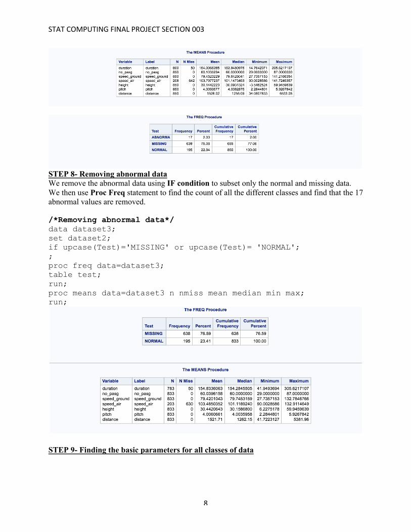
STEP 8- Removing abnormal data We remove the abnormal data using IF condition to subset only the normal and missing data. We then use Proc Freq statement to find the count of all the different classes and find that the 17 abnormal values are removed. /*Removing abnormal data*/ data dataset3; set dataset2; if upcase(Test)='MISSING' or upcase(Test)= 'NORMAL'; ; proc freq data=dataset3; table test; run; proc means data=dataset3 n nmiss mean median min max; run;
STEP 9- Finding the basic parameters for all classes of data

STATCOMPUTINGFINALPROJECTSECTION003
9
We find the basic parameters for all the classes of data using Proc Means statement again after sorting the data using Proc Sort by aircraft and by the test variables of missing and normal data. /*Finding the basic parameters for all classes of data*/ proc sort data=dataset3; by aircraft Test; run; proc means data=dataset3 n nmiss mean median min max; by aircraft Test; var duration no_pasg speed_ground speed_air height pitch distance; run;
CONCLUSION: We have now cleaned the data using different steps and iterations and have made the data ready for the next step of data analysis in accordance with CRISP DM methodology.

STATCOMPUTINGFINALPROJECTSECTION003
10
CHAPTER 2- DATA EXPLORATION GOAL: Data exploration is the second step in the process of data analysis and is an informative process to gain insights into the data that has been cleaned in the previous step. The process basically consists of variable identification as predictor and target variables and forming meaningful relationships between the classes of variables to understand the impact of variables. This stage involves creating the question which needs to be answered and identifying the information necessary to answer that particular question. The steps which have been used in this assignment are:
1. Plotting all the variables separated by the aircraft to understand the outliers and variation. 2. Plotting all the variables with distance to understand the effect of the variables on the
landing distance. 3. Finding the Correlation between the variables to understand the relationship
The steps may be reiterated multiple times to get a cleaner dataset when more variables are given or larger datasets are considered. STEP 1- Plotting all the variables separated by the aircraft to understand the outliers and variation. We use Proc boxplots on the dataset across all the variables with the aircraft type of Boeing and Airbus and the Insetgroup statement to have the data displayed in the box plots. We find there is a huge difference in the minimum value for distance between the aircrafts with Boeing having a higher minimum landing distance which is causing a marked change in the distribution of data. /*Plots for aircrafts*/ proc boxplot data=dataset3; plot (duration no_pasg speed_ground speed_air height pitch distance)*aircraft/ boxstyle = schematic nohlabel; insetgroup mean min max n nhigh nlow nout q1 q2 q3 range; run;

STATCOMPUTINGFINALPROJECTSECTION003
11

STATCOMPUTINGFINALPROJECTSECTION003
12

STATCOMPUTINGFINALPROJECTSECTION003
13
STEP 2- Plotting all the variables with distance to understand the effect of the variables on the landing distance. We use Proc Sgscatter and the Plot function to plot multiple plots of all the variables with distance in a single plot. We see a strong linear and positive relationship only for Speed_ground and Speed_air with the distance. /*Plots for distance*/ proc sgscatter data=dataset3; plot(duration no_pasg speed_ground speed_air height pitch aircraft)*distance; run;
STEP 3- Finding the Correlation between the variables to understand the relationship. We use Proc Corr to correlate the data by the variables to understand the correlation between the different variables pairwise. We find a strong correlation between distance and speed_air and speed_ground as expected from the plots. We also find that there is a correlation between speed_ground and speed_air which was shown before when understanding the missing data.

STATCOMPUTINGFINALPROJECTSECTION003
14
/*Correlation*/ proc corr data=dataset3; var duration no_pasg speed_ground speed_air height pitch distance; Title Pairwise Correlation Coefficients; run;
CONCLUSION: We have now explored the data in accordance with CRISP DM methodology using different steps and iterations and have understood the variables which have to be modelled to understand the relationship with landing distance which are- speed_air, speed_ground, height and pitch as their p values are less than 0.05 making statistically significant relationship.

STATCOMPUTINGFINALPROJECTSECTION003
15
CHAPTER 3 AND CHAPTER 4- MODELING AND MODEL CHECKING GOAL: Modeling is the third step in the process of data analysis and is used to model the predictor variables which are found to have an impact on the target variables found in the data exploration stage. In this step, typically various modeling techniques are selected and then applied and all the parameters calculated are then calibrated to obtain the optimal values. There are many modeling techniques which can be applied depending on the number of variables and the extent of data that is being provided. The steps which have been used in this assignment are:
1. Regression Analysis 2. Regression Analysis using significant variables 3. Regression Analysis using transformed variable 4. Check the distribution of residuals by plotting to check for independance 5. Check if the distribution of residuals is normally distributed 6. Perform hypothesis testing on the residuals
STEP 1- Using regression analysis on the distance variable with respect to all variables. We use Proc Reg to perform regression analysis for distance as response variable and all the remaining variables except aircraft as the predictor variables. We find that only 195 values were considered due to lot of missing values. We find p values below 0.05 level of significance for aircraft, speed_air and height showing statistically significant relationship with distance, which is also true from the correlation matrix. But we find no relation for speed_ground as found from correlation matrix as speed_ground and speed_air is highly correlated. We use speed_ground for further analysis as it does not have any missing values. We find that adjusted R square value is 0.9738 i.e. 97.38% of the variability is explained by this model. /*Regression Analysis*/ data dataset4; set dataset3; if aircraft='boeing' then aircraftcode = 0; else aircraftcode = 1; proc reg data=dataset4; model distance= aircraftcode duration no_pasg speed_ground speed_air height pitch ; title Regression analysis of the data set; run;

STATCOMPUTINGFINALPROJECTSECTION003
16

STATCOMPUTINGFINALPROJECTSECTION003
17
STEP 2- Using regression analysis using only significant variables. We use Proc Reg using only the three significant variables in the model. We find that 833 observations are now taken into account. The adjusted R square value predicts about 84% of the variability. We find all the variables are statistically significant for distance. /*Second iteration using significant variables*/ proc reg data=dataset4; model distance= aircraftcode speed_ground height; title Regression analysis of significant variables; run;

STATCOMPUTINGFINALPROJECTSECTION003
18
STEP 3- Regression analysis using transformed variable We use a new transformed variable for speed_ground which is a square of the variable in accordance with the transformation principles. We then use Proc Reg on the dataset with the four variables to achieve an optimum model. We get an adjusted R square of 97.60% to explain the variability for this model. We also find our assumptions of no relationship in residuals satisfied in the model. The final regression equation can be summed up as

STATCOMPUTINGFINALPROJECTSECTION003
19
y(distance)= 2230.448-399.37𝑥"+0.69815𝑥##- 69.97𝑥#+13.44𝑥$ where 𝑥"= make of an aircraft 𝑥# = ground speed of the aircraft 𝑥$ = height of the aircraft when passing over the run way. /*Third Iteration to achieve randomness of residuals*/ data dataset5; set dataset4; speed_ground_squared = speed_ground**2; proc reg data=dataset5; model distance= aircraftcode speed_ground_squared speed_ground height; title Regression analysis adjusting for speed_ground; run;

STATCOMPUTINGFINALPROJECTSECTION003
20
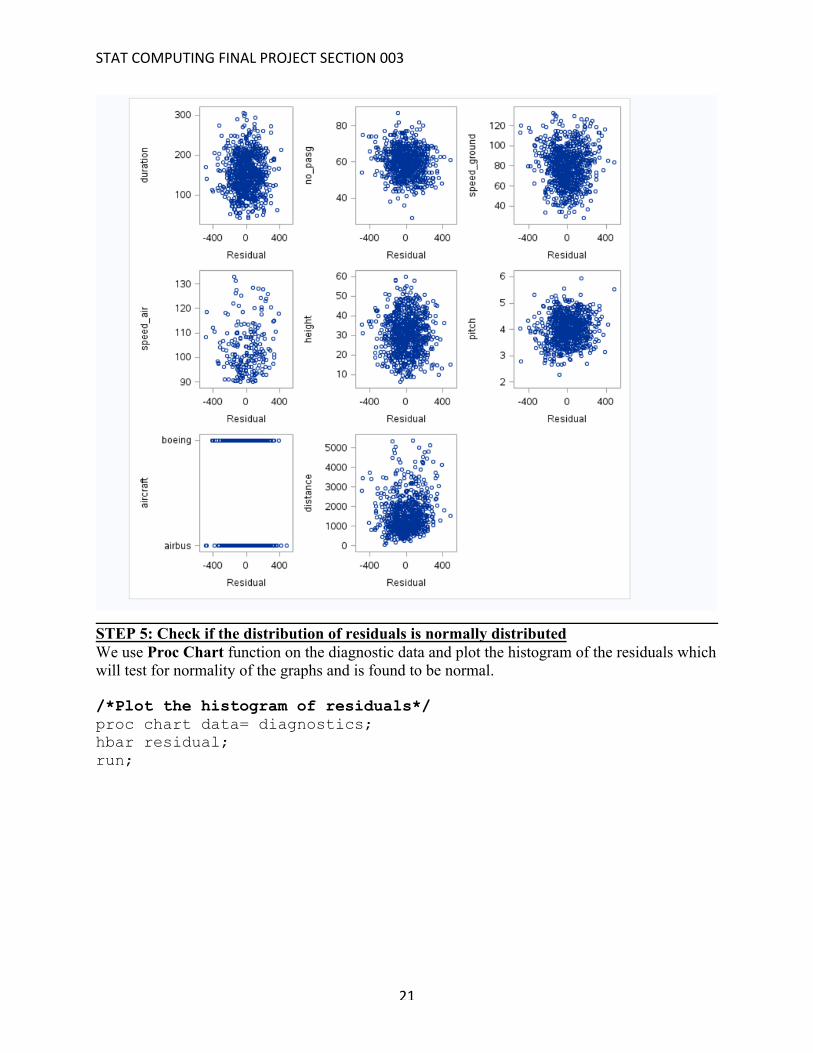
STEP 4: Check the distribution of residuals by plotting We can check the distribution of residuals by plotting all the residual against all the different variables using scatter plots. We don’t find any relationship being explained by the residuals which satisfies the first condition of error terms being independent. /*Plotting the residuals*/ proc sgscatter data=diagnostics; plot(duration no_pasg speed_ground speed_air height pitch aircraft distance)*residual; run;
STATCOMPUTINGFINALPROJECTSECTION003
21
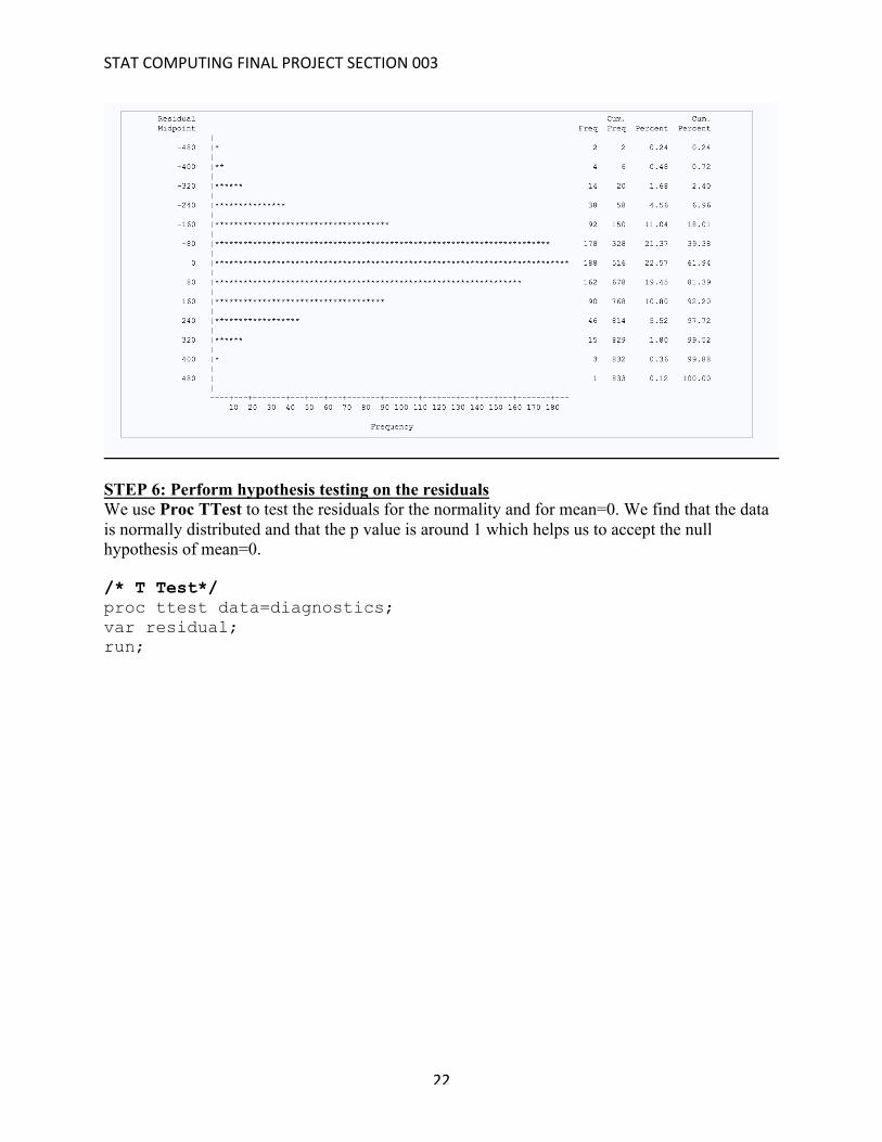
STEP 5: Check if the distribution of residuals is normally distributed We use Proc Chart function on the diagnostic data and plot the histogram of the residuals which will test for normality of the graphs and is found to be normal. /*Plot the histogram of residuals*/ proc chart data= diagnostics; hbar residual; run;
STATCOMPUTINGFINALPROJECTSECTION003
22
STEP 6: Perform hypothesis testing on the residuals We use Proc TTest to test the residuals for the normality and for mean=0. We find that the data is normally distributed and that the p value is around 1 which helps us to accept the null hypothesis of mean=0. /* T Test*/ proc ttest data=diagnostics; var residual; run;

STATCOMPUTINGFINALPROJECTSECTION003
23
CONCLUSION: We have now modeled and checked the model in accordance with CRISP DM methodology using different steps and iterations. We have also reframed our model with transformation to account for more variability and to also use predictor variables to define the relationship instead of the residuals. We find all the assumptions of the regression model satisfied which is
1. The error terms are independent. 2. The error terms are normally distributed. 3. Their mean is zero 4. They have constant variance.


