108
OR.A.SI © Orbit and Attitude Simulator Part I Antonios Arkas Flight Dynamics Engineer
| Date post: | 26-Jan-2017 |
| Category: |
Documents |
| Upload: | antonios-arkas |
| View: | 134 times |
| Download: | 2 times |
OR.A.SI © Orbit and Attitude
Simulator
Part I
Antonios Arkas Flight Dynamics Engineer
1.1 Orbit Determination

1.1.1 Orbit Determination Module Characteristics
Utilization of a batch weighted least-square estimator.
Enhancement of orbit determination accuracy with a priori information of the state
vector covariance matrix (Bayesian Estimation).
Radiation pressure coefficient Cp , ballistic coefficient and antenna biases for any
number of the Earth stations participating in the localization campaign, can be set as
solve-for parameters (provided that the problem formulation has good observability).
Raw measurement preprocessor for the reduction of noise.
Process of any kind of combination of tracking (azimuth-elevation) and/or range
measurements acquired from an arbitrary number of Earth stations.
Flexibility to configure the weighted least-square estimator with suitable choice
of the following parameters :
Combination of solve-for parameters.
Two different measurement rejection factors. One for the first number of
iterations and another for the subsequent iterations.
Maximum global WRMS (Weighted Root Mean Square) of residuals for
measurement rejection.
Minimum and maximum number of iterations.
Maximum number of divergent iterations.
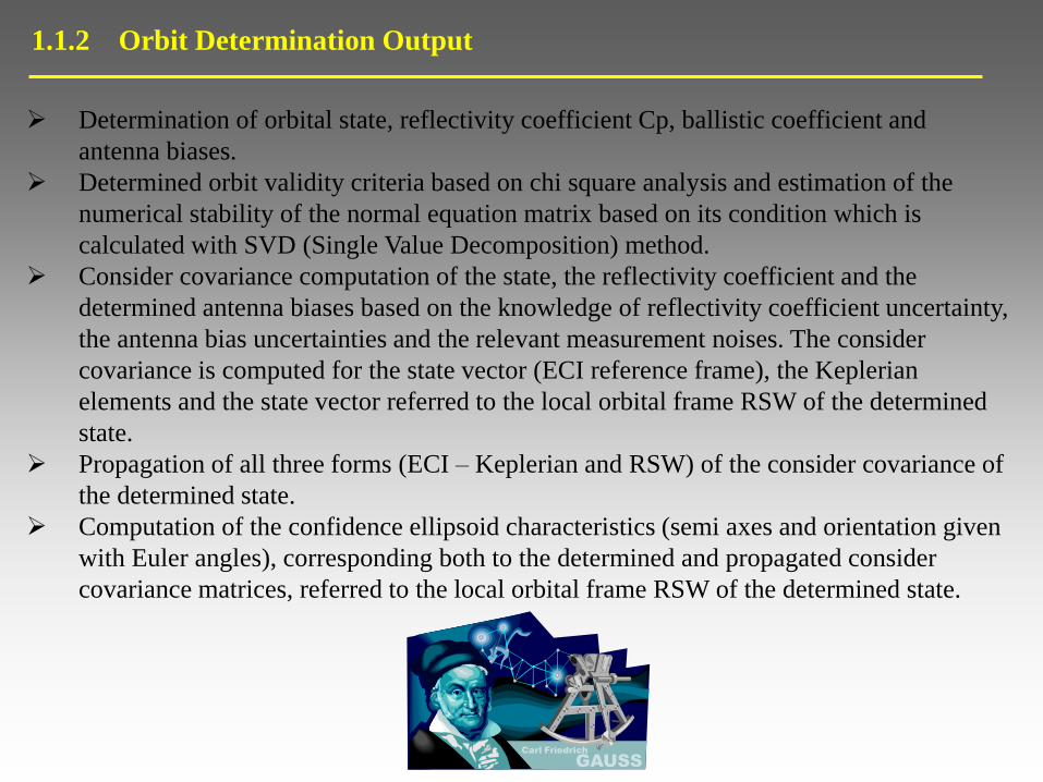
1.1.2 Orbit Determination Output
Determination of orbital state, reflectivity coefficient Cp, ballistic coefficient and
antenna biases.
Determined orbit validity criteria based on chi square analysis and estimation of the
numerical stability of the normal equation matrix based on its condition which is
calculated with SVD (Single Value Decomposition) method.
Consider covariance computation of the state, the reflectivity coefficient and the
determined antenna biases based on the knowledge of reflectivity coefficient uncertainty,
the antenna bias uncertainties and the relevant measurement noises. The consider
covariance is computed for the state vector (ECI reference frame), the Keplerian
elements and the state vector referred to the local orbital frame RSW of the determined
state.
Propagation of all three forms (ECI – Keplerian and RSW) of the consider covariance of
the determined state.
Computation of the confidence ellipsoid characteristics (semi axes and orientation given
with Euler angles), corresponding both to the determined and propagated consider
covariance matrices, referred to the local orbital frame RSW of the determined state.
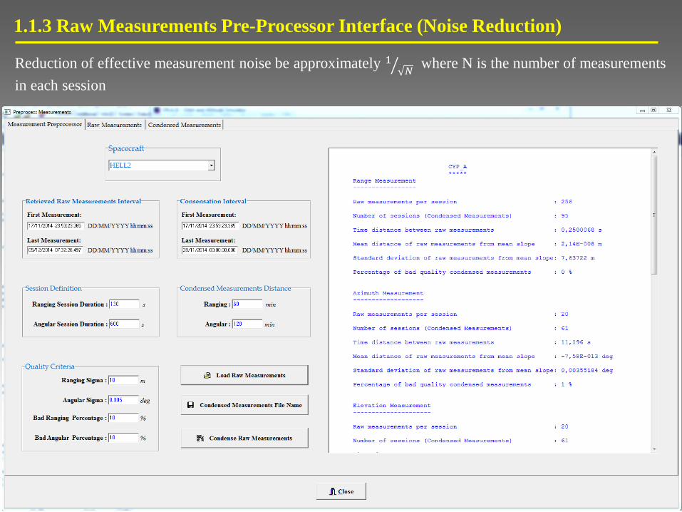
1.1.3 Raw Measurements Pre-Processor Interface (Noise Reduction)
Reduction of effective measurement noise be approximately 1𝑁 where N is the number of measurements
in each session
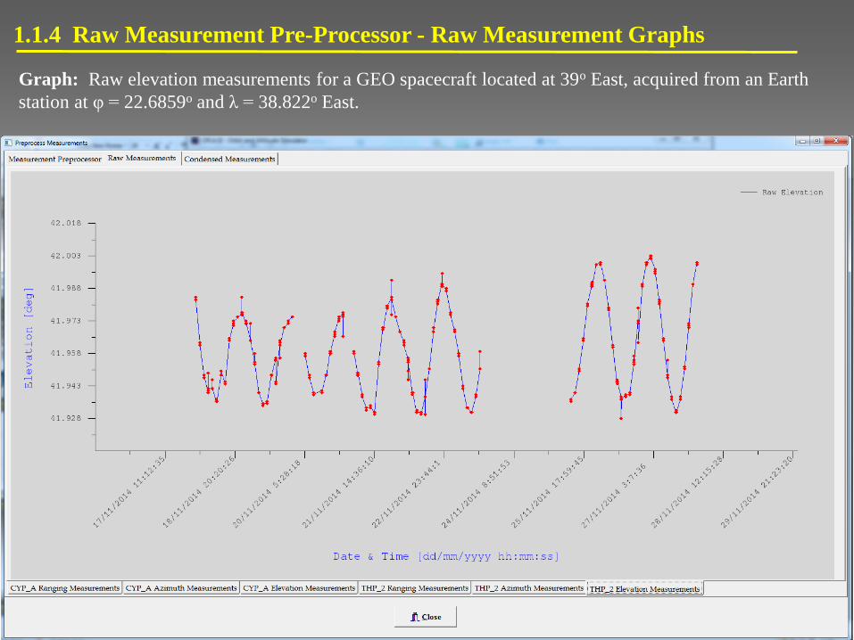
1.1.4 Raw Measurement Pre-Processor - Raw Measurement Graphs
Graph: Raw elevation measurements for a GEO spacecraft located at 39o East, acquired from an Earth
station at φ = 22.6859o and λ = 38.822o East.
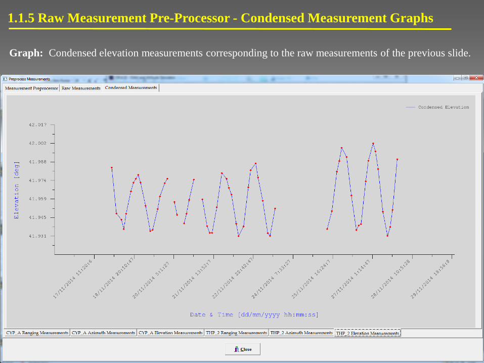
1.1.5 Raw Measurement Pre-Processor - Condensed Measurement Graphs
Graph: Condensed elevation measurements corresponding to the raw measurements of the previous slide.
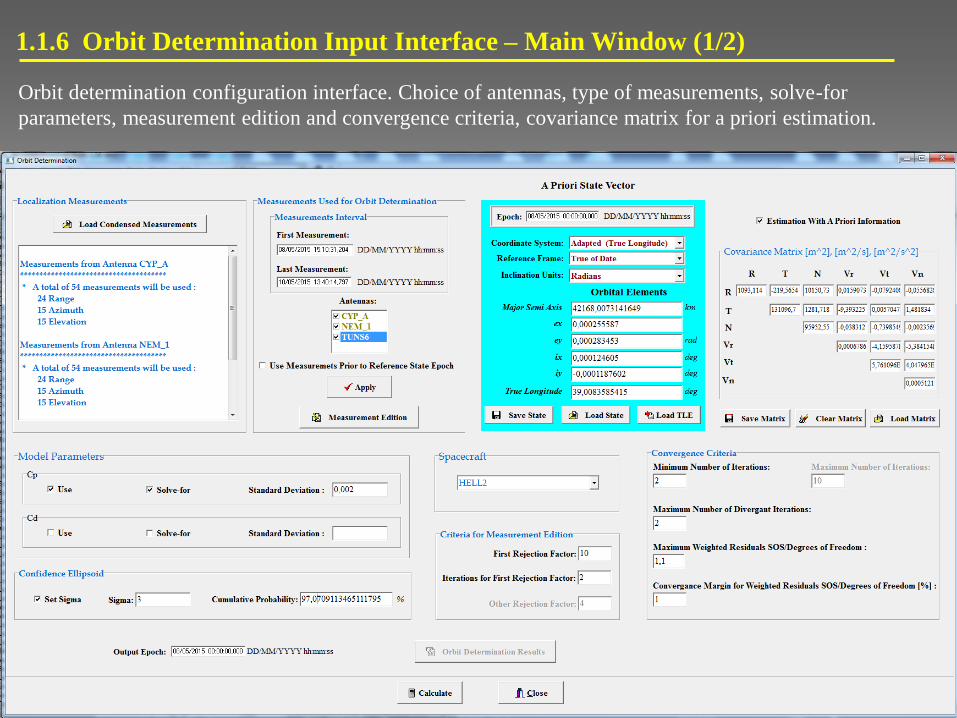
1.1.6 Orbit Determination Input Interface – Main Window (1/2)
Orbit determination configuration interface. Choice of antennas, type of measurements, solve-for
parameters, measurement edition and convergence criteria, covariance matrix for a priori estimation.

1.1.6 Orbit Determination Input Interface – Antenna Characteristics (1/2)
Selection of
1) antenna for localization measurements acquisition
2) antenna characteristics (noise and bias uncertainties for consider covariance analysis) and
3) antenna biases as solve-for parameters
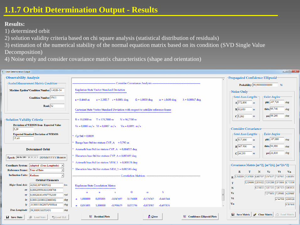
1.1.7 Orbit Determination Output - Results
Results:
1) determined orbit
2) solution validity criteria based on chi square analysis (statistical distribution of residuals)
3) estimation of the numerical stability of the normal equation matrix based on its condition (SVD Single Value
Decomposition)
4) Noise only and consider covariance matrix characteristics (shape and orientation)
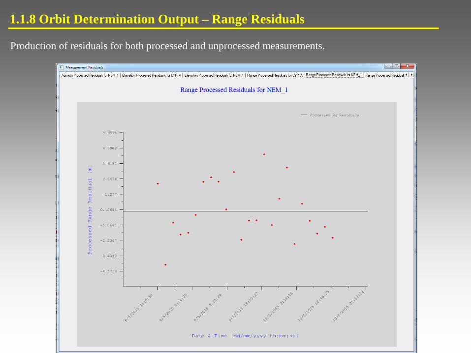
1.1.8 Orbit Determination Output – Range Residuals
Production of residuals for both processed and unprocessed measurements.

1.1.9 Orbit Determination Output - Confidence Ellipsoid Referred to the RSW Local Frame
1.2 Orbit Determination Validation
Comparison with COSMIC orbit determination. Actual measurements were acquired
from two distant antennas. From THP2 antenna both range and angular
measurements were used while from CYP antenna only range measurements were
used for orbit determination. COSMIC is the Flight Dynamics software for GEO
spacecrafts developed by AIRBUS (Former EADS-ASTRIUM).

1.2.1 Validation of Orbit Determination – Comparison with COSMIC Results (1/2)
Localization Campaign Characteristics
Localization measurements were acquired from two antennas :
Range, azimuth & elevation from Thermopylae station (THP) at Greece.
Range from Kakoratzia station (CYP) at Cyprus.
Number of sessions : 28
Time interval between sessions : 2 hours.
Solve-for parameters :
State vector.
Azimuth and elevation biases for Thermopylae station.
Range bias for Kakoratzia station.
Radiation pressure coefficient Cp.
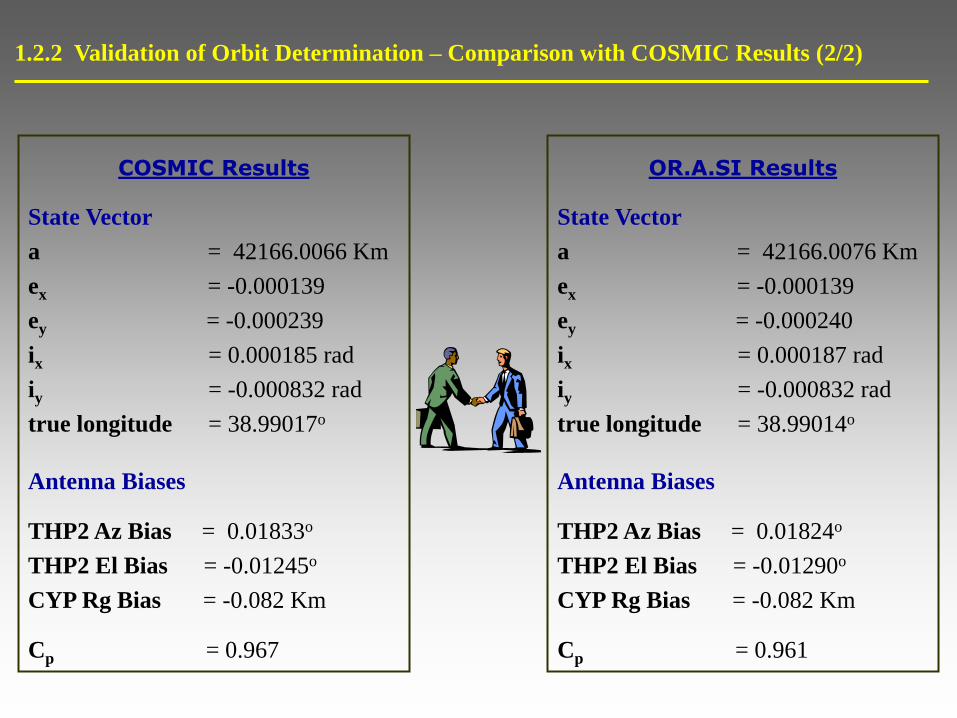
COSMIC Results
State Vector
a = 42166.0066 Km
ex = -0.000139
ey = -0.000239
ix = 0.000185 rad
iy = -0.000832 rad
true longitude = 38.99017o
Antenna Biases
THP2 Az Bias = 0.01833o
THP2 El Bias = -0.01245o
CYP Rg Bias = -0.082 Km
Cp = 0.967
OR.A.SI Results
State Vector
a = 42166.0076 Km
ex = -0.000139
ey = -0.000240
ix = 0.000187 rad
iy = -0.000832 rad
true longitude = 38.99014o
Antenna Biases
THP2 Az Bias = 0.01824o
THP2 El Bias = -0.01290o
CYP Rg Bias = -0.082 Km
Cp = 0.961
1.2.2 Validation of Orbit Determination – Comparison with COSMIC Results (2/2)

Range Residuals for Both Antennas
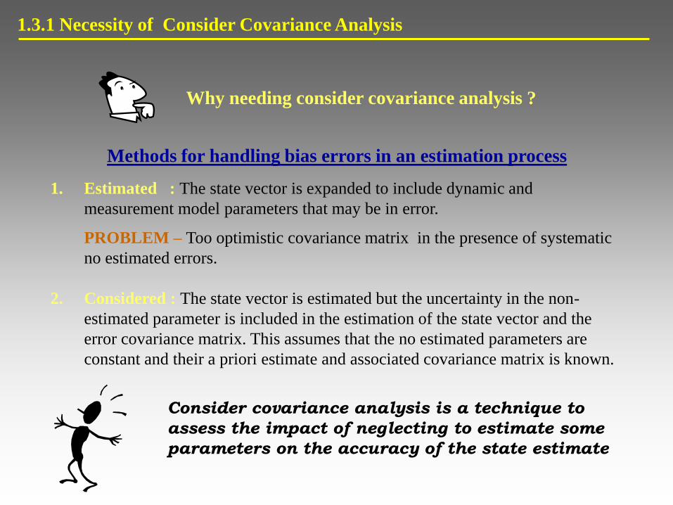
Why needing consider covariance analysis ?
Methods for handling bias errors in an estimation process
1. Estimated : The state vector is expanded to include dynamic and
measurement model parameters that may be in error.
PROBLEM – Too optimistic covariance matrix in the presence of systematic
no estimated errors.
2. Considered : The state vector is estimated but the uncertainty in the non-
estimated parameter is included in the estimation of the state vector and the
error covariance matrix. This assumes that the no estimated parameters are
constant and their a priori estimate and associated covariance matrix is known.
Consider covariance analysis is a technique to
assess the impact of neglecting to estimate some
parameters on the accuracy of the state estimate
1.3.1 Necessity of Consider Covariance Analysis
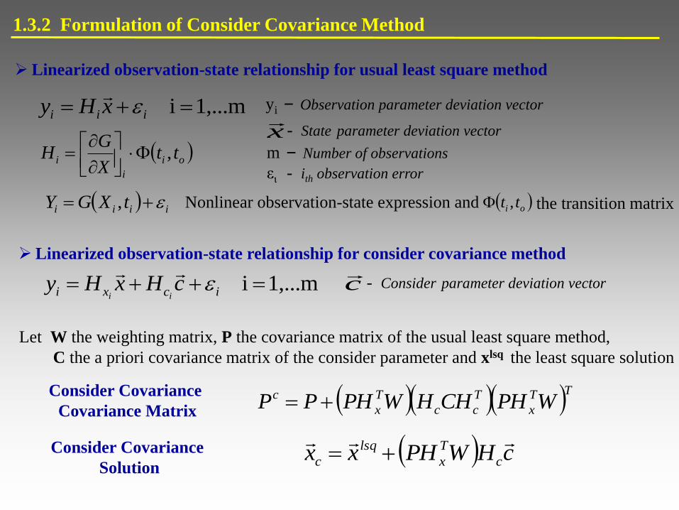
1.3.2 Formulation of Consider Covariance Method
1,...mi iii xHy
Linearized observation-state relationship for usual least square method
yi – Observation parameter deviation vector
x
- State parameter deviation vector
m – Number of observations
ει - ith observation error
Linearized observation-state relationship for consider covariance method
1,...mi icxi cHxHyii
c
- Consider parameter deviation vector
Let W the weighting matrix, P the covariance matrix of the usual least square method,
C the a priori covariance matrix of the consider parameter and xlsq the least square solution
TT
x
T
cc
T
x
c WPHCHHWPHPP Consider Covariance
Covariance Matrix
Consider Covariance
Solution cHWPHxx c
T
x
lsq
c
oi
i
i ttX
GH ,
iiii tXGY , Nonlinear observation-state expression and oi tt , the transition matrix
1.4 Formal Consider Covariance
Validation
Monte Carlo Orbit Determination:
Simulate range and angular localization measurements with Gaussian noise, from two
distant antennas. Incorporation of Gaussian uncertainty in the antenna biases and
subsequent orbit determination. Comparison of the formal covariance matrix with
the sample covariance matrix computed from the descriptive statistics of the Monte
Carlo orbit determination iterations.
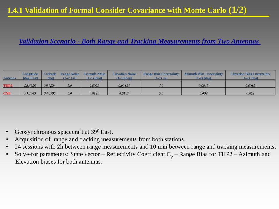
1.4.1 Validation of Formal Consider Covariance with Monte Carlo (1/2)
Validation Scenario - Both Range and Tracking Measurements from Two Antennas
Antenna
Longitude
[deg East]
Latitude
[deg]
Range Noise
(1-σ) [m]
Azimuth Noise
(1-σ) [deg]
Elevation Noise
(1-σ) [deg]
Range Bias Uncertainty
(1-σ) [m]
Azimuth Bias Uncertainty
(1-σ) [deg]
Elevation Bias Uncertainty
(1-σ) [deg]
THP2 22.6859 38.8224 5.0 0.0023 0.00124 6.0 0.0015 0.0015
CYP 33.3843 34.8592 5.0 0.0129 0.0137 5.0 0.002 0.002
• Geosynchronous spacecraft at 390 East.
• Acquisition of range and tracking measurements from both stations.
• 24 sessions with 2h between range measurements and 10 min between range and tracking measurements.
• Solve-for parameters: State vector – Reflectivity Coefficient Cp – Range Bias for THP2 – Azimuth and
Elevation biases for both antennas.
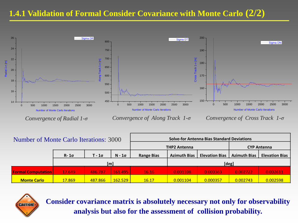
1.4.1 Validation of Formal Consider Covariance with Monte Carlo (2/2)
Solve-for Antenna Bias Standard Deviations
THP2 Antenna CYP Antenna
R- 1σ T - 1σ N - 1σ Range Bias Azimuth Bias Elevation Bias Azimuth Bias Elevation Bias
[m] [deg]
Formal Computation 17.649 486.787 161.495 16.16 0.001108 0.000363 0.002722 0.002611
Monte Carlo 17.869 487.866 162.529 16.17 0.001104 0.000357 0.002743 0.002598
Number of Monte Carlo Iterations: 3000
0 500 1000 1500 2000 2500 3000
14
16
18
20
22
24
26
Radia
l 1-[m
]
Number of Monte Carlo Iterations
Sigma DR
Convergence of Radial 1-σ
0 500 1000 1500 2000 2500 3000
450
500
550
600
650
700
750
800
Alo
ng T
rack 1
-[m
]
Number of Monte Carlo Iterations
Sigma DT
Convergence of Along Track 1-σ
Consider covariance matrix is absolutely necessary not only for observability
analysis but also for the assessment of collision probability.
0 500 1000 1500 2000 2500 3000
150
160
170
180
190
200
Cro
ss T
rack 1
-[m
]
Number of Monte Carlo Iterations
Sigma DN
Convergence of Cross Track 1-σ

1.5 Case Studies of Various Orbit
Determination Setups Based on
Consider Covariance Analysis
Case Studies for Consider Covariance Analysis – GEO Spacecraft at 39o East (1/2)
Antenna Diameter [m] λ [deg] φ [deg] h [m] σρ [m] σΑ,Ε [deg] σΔρ [m] σΔΑ,ΔΕ [deg]
THP 31 22.68 38.82 70 5 0.003 20 0.004
CYP 4,8 33.384 34.85 215 3 0.02 20 0.03
σR [m] σT [m] σN [m] σVr [m/s] σVt [m/s] σVn [m/s] σa [m]
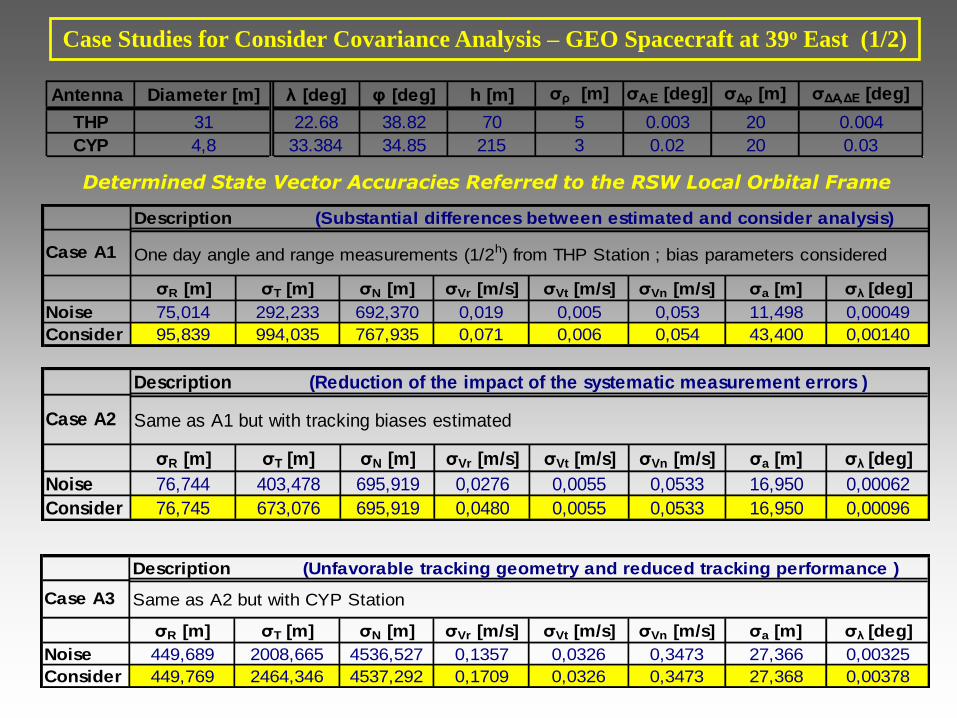
Noise 75,014 292,233 692,370 0,019 0,005 0,053 11,498
Consider 95,839 994,035 767,935 0,071 0,006 0,054 43,400
0,00049
0,00140
Description (Substantial differences between estimated and consider analysis)
Case A1 One day angle and range measurements (1/2h) from THP Station ; bias parameters considered
σλ [deg]
σR [m] σT [m] σN [m] σVr [m/s] σVt [m/s] σVn [m/s] σa [m]
Noise 76,744 403,478 695,919 0,0276 0,0055 0,0533 16,950
Consider 76,745 673,076 695,919 0,0480 0,0055 0,0533 16,950
0,00062
0,00096
Description (Reduction of the impact of the systematic measurement errors )
Case A2 Same as A1 but with tracking biases estimated
σλ [deg]
Determined State Vector Accuracies Referred to the RSW Local Orbital Frame
σR [m] σT [m] σN [m] σVr [m/s] σVt [m/s] σVn [m/s] σa [m]
Noise 449,689 2008,665 4536,527 0,1357 0,0326 0,3473 27,366
Consider 449,769 2464,346 4537,292 0,1709 0,0326 0,3473 27,368
0,00325
0,00378
Description (Unfavorable tracking geometry and reduced tracking performance )
Case A3 Same as A2 but with CYP Station
σλ [deg]
Case Studies for Consider Covariance Analysis – GEO Spacecraft at 39o East (2/2)
σR [m] σT [m] σN [m] σVr [m/s] σVt [m/s] σVn [m/s] σa [m]
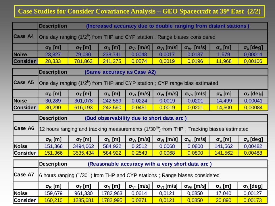
Noise 23,827 79,030 238,741 0,0048 0,0017 0,0187 1,579
Consider 28,333 781,862 241,275 0,0574 0,0019 0,0196 11,968
0,00014
0,00106
Description (Increased accuracy due to double ranging from distant stations )
Case A4 One day ranging (1/2h) from THP and CYP station ; Range biases considered
σλ [deg]
σR [m] σT [m] σN [m] σVr [m/s] σVt [m/s] σVn [m/s] σa [m]
Noise 30,289 301,078 242,589 0,0224 0,0019 0,0201 14,499
Consider 30,290 616,193 242,590 0,0451 0,0019 0,0201 14,500
0,00041
0,00084
Description (Same accuracy as Case A2)
Case A5 One day ranging (1/2h) from THP and CYP station ; CYP range bias estimated
σλ [deg]
σR [m] σT [m] σN [m] σVr [m/s] σVt [m/s] σVn [m/s] σa [m]
Noise 151,366 3494,062 584,922 0,2512 0,0068 0,0800 141,562
Consider 151,366 3535,434 584,922 0,2543 0,0068 0,0800 141,562
0,00482
0,00488
Description (Bud observability due to short data arc )
Case A6 12 hours ranging and tracking measurements (1/30m) from THP ; Tracking biases estimated
σλ [deg]
σR [m] σT [m] σN [m] σVr [m/s] σVt [m/s] σVn [m/s] σa [m]
Noise 159,679 961,330 1782,963 0,0614 0,0121 0,0850 17,040
Consider 160,210 1285,681 1782,995 0,0871 0,0121 0,0850 20,890
0,00127
0,00173
Description (Reasonable accuracy with a very short data arc )
Case A7 6 hours ranging (1/30m) from THP and CYP stations ; Range biases considered
σλ [deg]
1.6. Condition Number, Observability
And Relevance With
Orbit Determination Error Variance
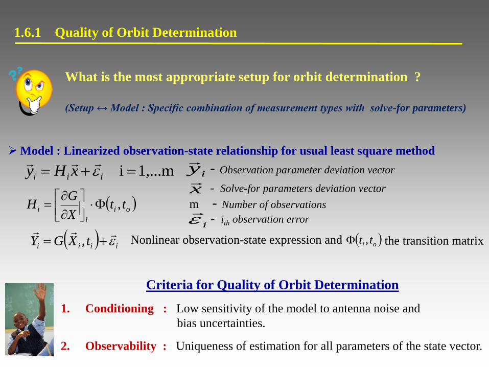
What is the most appropriate setup for orbit determination ?
(Setup ↔ Model : Specific combination of measurement types with solve-for parameters)
Criteria for Quality of Orbit Determination
1. Conditioning : Low sensitivity of the model to antenna noise and
bias uncertainties.
2. Observability : Uniqueness of estimation for all parameters of the state vector.
1,...mi iii xHy
Model : Linearized observation-state relationship for usual least square method
- Observation parameter deviation vector
x
- Solve-for parameters deviation vector
m - Number of observations
- ith observation error
oi
i
i ttX
GH ,
iiii tXGY
, Nonlinear observation-state expression and oi tt , the transition matrix
iy
i
1.6.1 Quality of Orbit Determination
1.6.2 Conditioning and Observability (1/2)
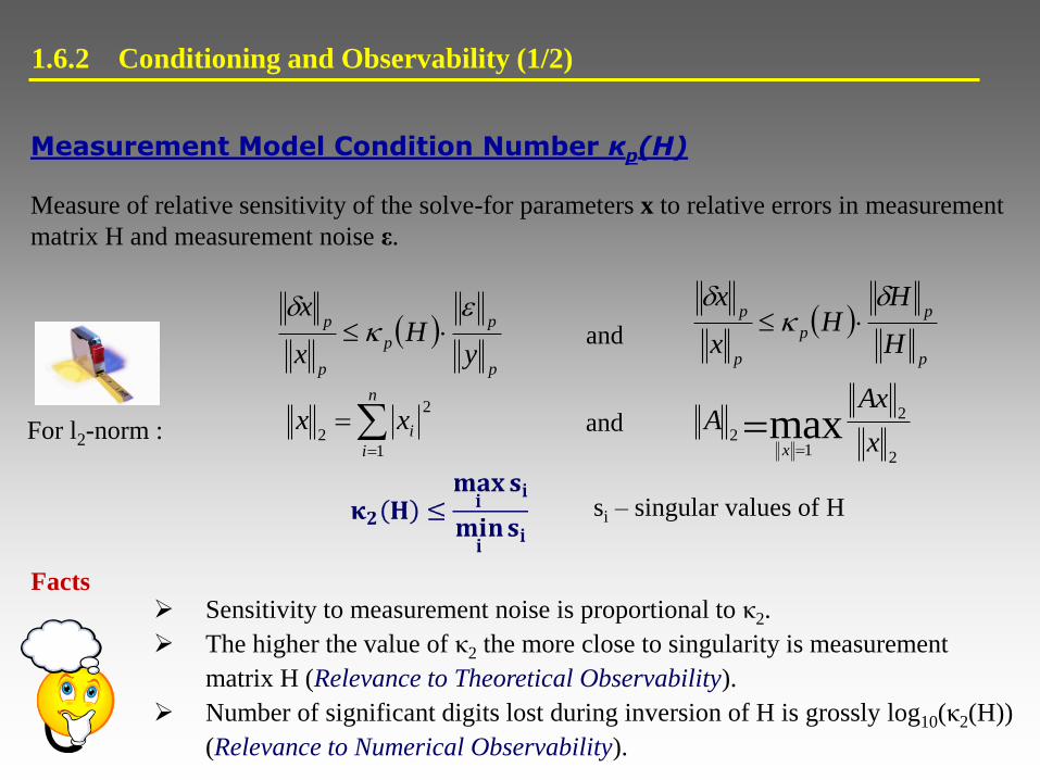
Measurement Model Condition Number κp(Η)
Measure of relative sensitivity of the solve-for parameters x to relative errors in measurement
matrix H and measurement noise ε.
Facts Sensitivity to measurement noise is proportional to κ2.
The higher the value of κ2 the more close to singularity is measurement
matrix H (Relevance to Theoretical Observability).
Number of significant digits lost during inversion of H is grossly log10(κ2(H))
(Relevance to Numerical Observability).
For l2-norm : and
si – singular values of H
and p
p
p
p
p
yH
x
x
p
p
p
p
p
H
HH
x
x
n
i
ixx1
2
2
2
2
12 max
x
AxA
x
1.6.3 Conditioning and Observability (2/2)
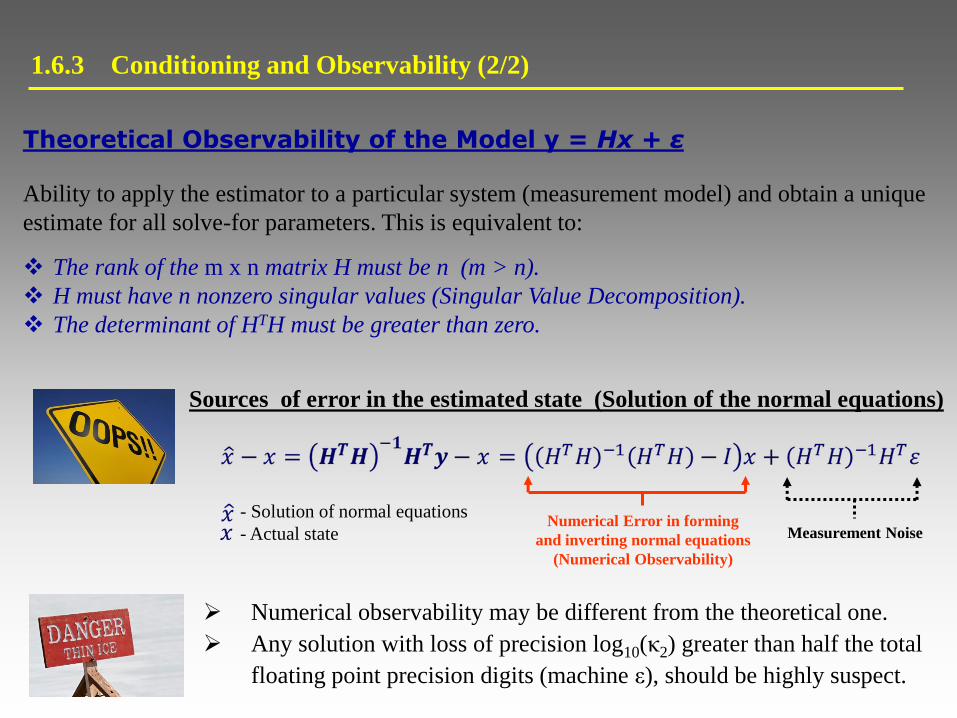
Theoretical Observability of the Model y = Ηx + ε
Ability to apply the estimator to a particular system (measurement model) and obtain a unique
estimate for all solve-for parameters. This is equivalent to:
The rank of the m x n matrix H must be n (m > n).
H must have n nonzero singular values (Singular Value Decomposition).
The determinant of HTH must be greater than zero.
Measurement Noise Numerical Error in forming
and inverting normal equations
(Numerical Observability)
Sources of error in the estimated state (Solution of the normal equations)
- Solution of normal equations
- Actual state
Numerical observability may be different from the theoretical one.
Any solution with loss of precision log10(κ2) greater than half the total
floating point precision digits (machine ε), should be highly suspect.
1.6.3 Observability Analysis Module Characteristics (1/2)
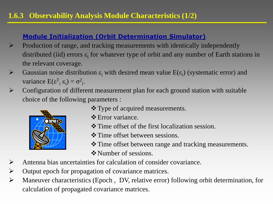
Module Initialization (Orbit Determination Simulator)
Production of range, and tracking measurements with identically independently
distributed (iid) errors εi for whatever type of orbit and any number of Earth stations in
the relevant coverage.
Gaussian noise distribution εi with desired mean value E(εi) (systematic error) and
variance E(εΤi εi) = σ2
i.
Configuration of different measurement plan for each ground station with suitable
choice of the following parameters :
Type of acquired measurements.
Error variance.
Time offset of the first localization session.
Time offset between sessions.
Time offset between range and tracking measurements.
Number of sessions.
Antenna bias uncertainties for calculation of consider covariance.
Output epoch for propagation of covariance matrices.
Maneuver characteristics (Epoch , DV, relative error) following orbit determination, for
calculation of propagated covariance matrices.
1.6.4 Observability Analysis Module Characteristics (2/2)
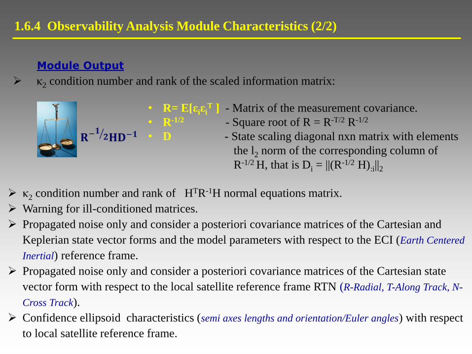
κ2 condition number and rank of HTR-1H normal equations matrix.
Warning for ill-conditioned matrices.
Propagated noise only and consider a posteriori covariance matrices of the Cartesian and
Keplerian state vector forms and the model parameters with respect to the ECI (Earth Centered
Inertial) reference frame.
Propagated noise only and consider a posteriori covariance matrices of the Cartesian state
vector form with respect to the local satellite reference frame RTN (R-Radial, T-Along Track, N-
Cross Track).
Confidence ellipsoid characteristics (semi axes lengths and orientation/Euler angles) with respect
to local satellite reference frame.
Module Output
κ2 condition number and rank of the scaled information matrix:
• R= E[εiεiT ] - Matrix of the measurement covariance.
• R-1/2 - Square root of R = R-T/2 R-1/2
• D - State scaling diagonal nxn matrix with elements
the l2 norm of the corresponding column of
R-1/2 H, that is Di = ||(R-1/2 H):i||2
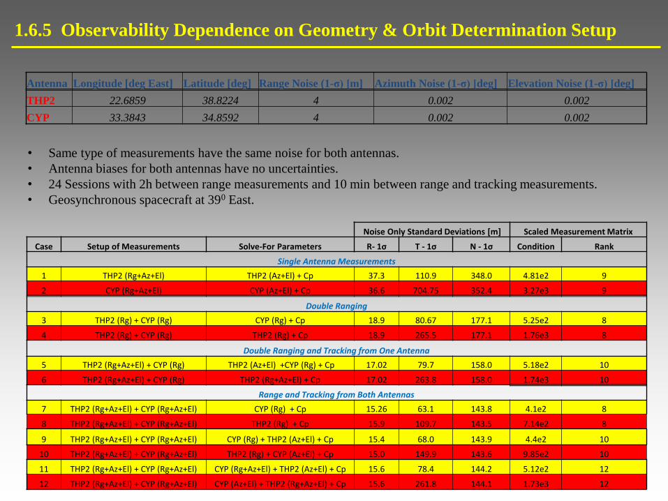
1.6.5 Observability Dependence on Geometry & Orbit Determination Setup
Antenna Longitude [deg East] Latitude [deg] Range Noise (1-σ) [m] Azimuth Noise (1-σ) [deg] Elevation Noise (1-σ) [deg]
THP2 22.6859 38.8224 4 0.002 0.002
CYP 33.3843 34.8592 4 0.002 0.002
• Same type of measurements have the same noise for both antennas.
• Antenna biases for both antennas have no uncertainties.
• 24 Sessions with 2h between range measurements and 10 min between range and tracking measurements.
• Geosynchronous spacecraft at 390 East.
Noise Only Standard Deviations [m] Scaled Measurement Matrix
Case Setup of Measurements Solve-For Parameters R- 1σ T - 1σ N - 1σ Condition Rank
Single Antenna Measurements
1 THP2 (Rg+Az+El) THP2 (Az+El) + Cp 37.3 110.9 348.0 4.81e2 9
2 CYP (Rg+Az+El) CYP (Az+El) + Cp 36.6 704.75 352.4 3.27e3 9
Double Ranging
3 THP2 (Rg) + CYP (Rg) CYP (Rg) + Cp 18.9 80.67 177.1 5.25e2 8
4 THP2 (Rg) + CYP (Rg) THP2 (Rg) + Cp 18.9 265.5 177.1 1.76e3 8
Double Ranging and Tracking from One Antenna
5 THP2 (Rg+Az+El) + CYP (Rg) THP2 (Az+El) +CYP (Rg) + Cp 17.02 79.7 158.0 5.18e2 10
6 THP2 (Rg+Az+El) + CYP (Rg) THP2 (Rg+Az+El) + Cp 17.02 263.8 158.0 1.74e3 10
Range and Tracking from Both Antennas
7 THP2 (Rg+Az+El) + CYP (Rg+Az+El) CYP (Rg) + Cp 15.26 63.1 143.8 4.1e2 8
8 THP2 (Rg+Az+El) + CYP (Rg+Az+El) THP2 (Rg) + Cp 15.9 109.7 143.5 7.14e2 8
9 THP2 (Rg+Az+El) + CYP (Rg+Az+El) CYP (Rg) + THP2 (Az+El) + Cp 15.4 68.0 143.9 4.4e2 10
10 THP2 (Rg+Az+El) + CYP (Rg+Az+El) THP2 (Rg) + CYP (Az+El) + Cp 15.0 149.9 143.6 9.85e2 10
11 THP2 (Rg+Az+El) + CYP (Rg+Az+El) CYP (Rg+Az+El) + THP2 (Az+El) + Cp 15.6 78.4 144.2 5.12e2 12
12 THP2 (Rg+Az+El) + CYP (Rg+Az+El) CYP (Az+El) + THP2 (Rg+Az+El) + Cp 15.6 261.8 144.1 1.73e3 12
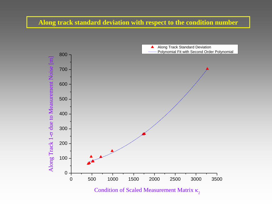
Along track standard deviation with respect to the condition number
0 500 1000 1500 2000 2500 3000 3500
0
100
200
300
400
500
600
700
800A
long T
rack
1-d
ue
to M
easu
rem
ent
Nois
e [m
] Along Track Standard Deviation
Polynomial Fit with Second Order Polynomial
Condition of Scaled Measurement Matrix
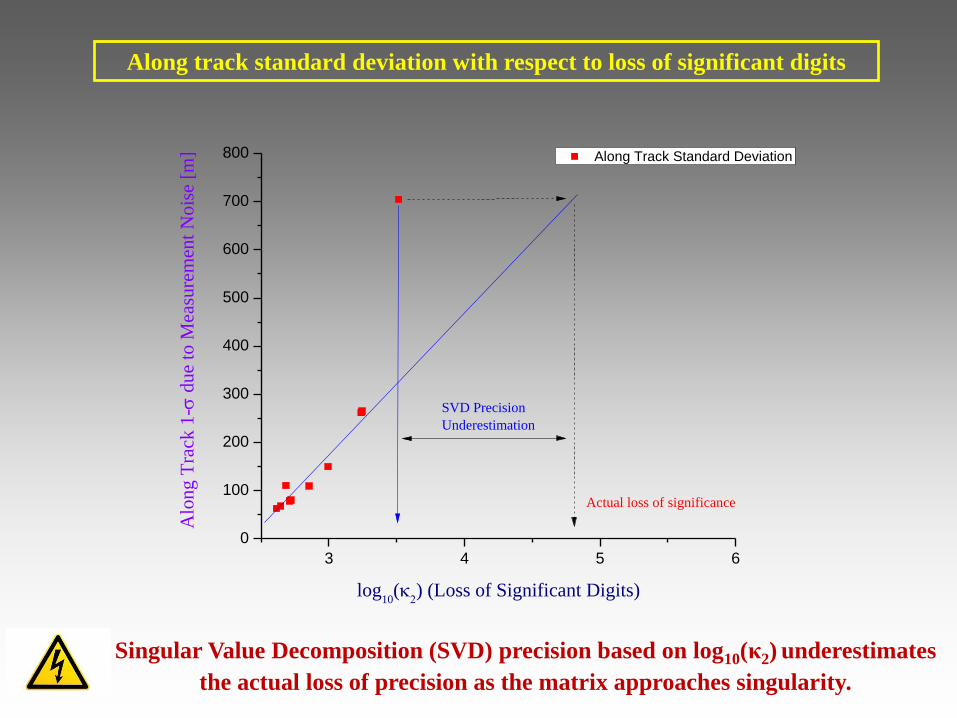
Along track standard deviation with respect to loss of significant digits
Singular Value Decomposition (SVD) precision based on log10(κ2) underestimates
the actual loss of precision as the matrix approaches singularity.
3 4 5 6
0
100
200
300
400
500
600
700
800
Alo
ng T
rack
1-d
ue
to M
easu
rem
ent
Nois
e [m
] Along Track Standard Deviation
log10
() (Loss of Significant Digits)
Actual loss of significance
SVD Precision
Underestimation

• 24 Sessions with 2h between range measurements and 10 min between range and tracking measurements.
• Geosynchronous spacecraft at 390 East.
1.6.6 Observability, Consider Covariance & Quality of Orbit Determination (1/2)
Antenna
Longitude
[deg East]
Latitude
[deg]
Range Noise
(1-σ) [m]
Azimuth Noise
(1-σ) [deg]
Elevation Noise
(1-σ) [deg]
Range Bias Uncertainty
(1-σ) [m]
Azimuth Bias Uncertainty
(1-σ) [deg]
Elevation Bias Uncertainty
(1-σ) [deg]
THP2 22.6859 38.8224 4.23 0.003 0.0017 11.4 0.0015 0.0015
CYP 33.3843 34.8592 3.4 0.0147 0.0112 5 0.0025 0.0025
Noise Only Standard Deviations [m] Consider Analysis Standard Deviations [m] Scaled Measurement Matrix
Case Setup of Measurements Solve-For Parameters R- 1σ T - 1σ N - 1σ R- 1σ T - 1σ N - 1σ Condition Rank
Single Antenna Measurements
1 THP2 (Rg+Az+El) THP2 (Az+El) + Cp 34.7 110.6 323.6 34.7 327.1 323.6 4.5e2 9
2 CYP (Rg+Az+El) CYP (Az+El) + Cp 198.6 743.8 2021.4 198.5 825.2 2021.5 3.7e3 9
Double Ranging
3 THP2 (Rg) + CYP (Rg) CYP (Rg) + Cp 18.1 81.5 169.4 18.1 318.4 169.4 5.7e2 8
4 THP2 (Rg) + CYP (Rg) THP2 (Rg) + Cp 18.1 268.5 169.4 18.1 449.4 169.4 1.9e3 8
Double Ranging and Tracking from One Antenna
5 THP2 (Rg+Az+El) + CYP (Rg) THP2 (Az+El) +CYP (Rg) + Cp 16.2 80.4 150.1 16.2 318.12 150.1 5.6e2 10
6 THP2 (Rg+Az+El) + CYP (Rg) THP2 (Rg+Az+El) + Cp 16.1 267.5 150.1 16.1 448.9 150.1 1.9e3 10
Range and Tracking from Both Antennas
7 THP2 (Rg+Az+El) + CYP (Rg+Az+El) CYP (Rg) + Cp 16.0 75.3 149.6 17 298.4 150.7 5.3e2 8
8 THP2 (Rg+Az+El) + CYP (Rg+Az+El) THP2 (Rg) + Cp 15.6 182.0 149.2 17.8 453.7 151.44 1.3e3 8
9 THP2 (Rg+Az+El) + CYP (Rg+Az+El) CYP (Rg) + THP2 (Az+El) + Cp 16.1 80.1 149.7 16.1 316.5 149.7 5.6e2 10
10 THP2 (Rg+Az+El) + CYP (Rg+Az+El) THP2 (Rg) + CYP (Az+El) + Cp 15.6 184.35 149.2 17.9 464.7 151.5 1.3e3 10
11 THP2 (Rg+Az+El) + CYP (Rg+Az+El) CYP (Rg+Az+El) + THP2 (Az+El) + Cp 16.1 80.4 149.7 16.1 318.1 149.7 5.7e2 12
12 THP2 (Rg+Az+El) + CYP (Rg+Az+El) CYP (Az+El) + THP2 (Rg+Az+El) + Cp 16.1 267.3 149.7 16.1 448.8 149.7 1.9e3 12

1.6.7 Observability, Consider Covariance & Quality of Orbit Determination (2/2)
Observability primarily depends on the geometry of the Earth stations participating in
the localization campaign and the orbit determination setup.
Since observability is directly connected to the variance of the along track error, the
Flight Dynamics Engineer can detect the best possible orbit determination setup by
comparing the aforementioned variance corresponding to each different setup.
Observability can’t guarantee best orbit determination performance due to the
additional error dispersion introduced by the uncertainty of the consider parameters.
Conclusions
2,6 2,8 3,0 3,2 3,4 3,6 3,8 4,0 4,2 4,4 4,6 4,8 5,0
0
200
400
600
800
Alo
ng
Tra
ck 1
-d
ue
to M
easu
rem
ent
No
ise
[m]
Actual loss of
significance
log10
() (Loss of Significant Digits)
Along Track Standard Deviation
SVD Precision
Underestimation
0 500 1000 1500 2000 2500 3000 3500 4000
0
100
200
300
400
500
600
700
800
Alo
ng
Tra
ck 1
-d
ue
to M
easu
rem
ent
No
ise
[m]
Condition of Scaled Measurement Matrix
Along Track Standard Deviation
Second Order Polynomial Fit
Equation
y = Intercept + B1*x^1 + B2*x^2
Weight No Weighting
Residual Sum of Squares
1641,0144
Adj. R-Square 0,99487
Value Standard Error
Along Track St Intercept 53,69291 11,0751
Along Track St B1 0,03935 0,01504
Along Track St B2 3,97067E-5 3,82244E-6
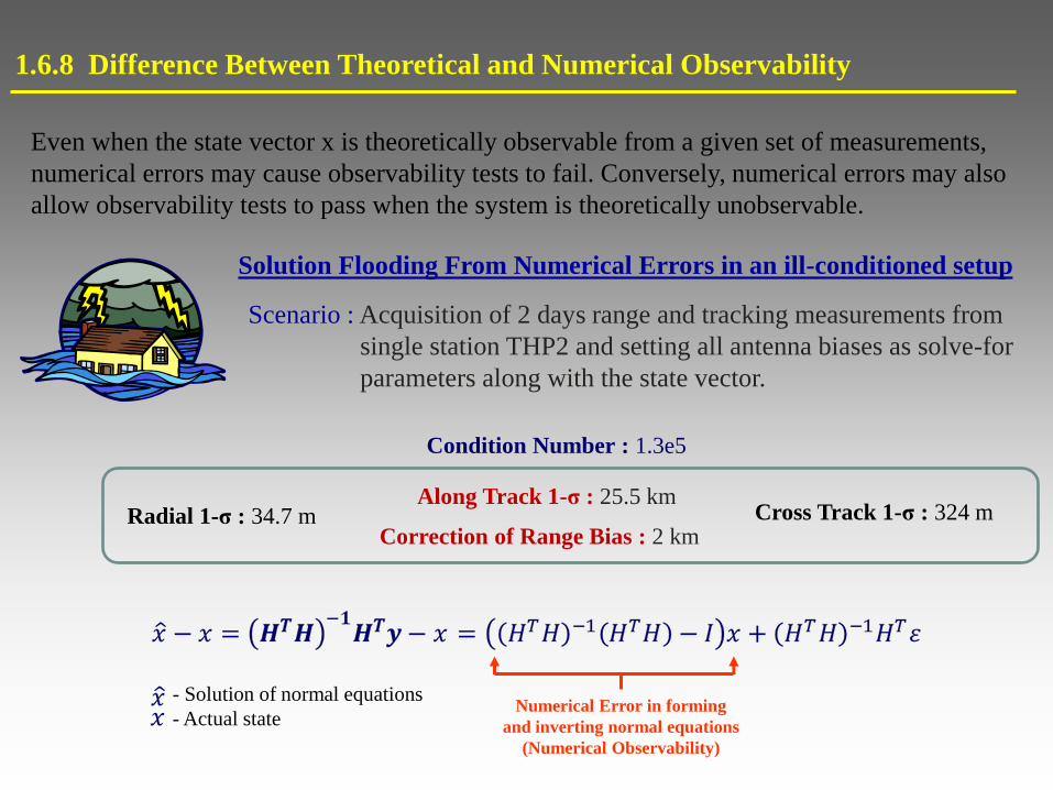
1.6.8 Difference Between Theoretical and Numerical Observability
Even when the state vector x is theoretically observable from a given set of measurements,
numerical errors may cause observability tests to fail. Conversely, numerical errors may also
allow observability tests to pass when the system is theoretically unobservable.
Solution Flooding From Numerical Errors in an ill-conditioned setup
Scenario : Acquisition of 2 days range and tracking measurements from
single station THP2 and setting all antenna biases as solve-for
parameters along with the state vector.
- Solution of normal equations
- Actual state Numerical Error in forming
and inverting normal equations
(Numerical Observability)
Along Track 1-σ : 25.5 km
Correction of Range Bias : 2 km Radial 1-σ : 34.7 m Cross Track 1-σ : 324 m
Condition Number : 1.3e5

2.1 Propagation Module

2.1.1 Propagation Module Characteristics (1/2)
Three alternative numerical integrators for orbit propagation of perturbed orbits and
two analytic propagators:
Continuous embedded 4th order Runge-Kutta-Fehelberg method RKF4(5), with adaptive
step size control.
Continuous embedded 8th order Runge-Kutta Dormant-Prince method RKF8(7)-13,
with adaptive step size control.
m-th order Adams-Moulton predictor-corrector method with dense output based on m-th
order Lagrange interpolator.
SGP4/SDP4 propagator for TLE elements (Spacetrack Report No.03).
Analytic solution of the restricted two body problem for unperturbed orbits.
Estimation of the numerical propagator global truncation error in accordance to the
characteristics of the propagator and the type of orbit (eccentricity) which is propagated.
Forward and backward propagation of all types of closed orbits while taking account a
series of triaxial impulsive, continuous thrust maneuvers or a mix of these two type of
maneuvers.
The propagator accounts for the following perturbations:
Sun and Moon gravity.
Earth potential according to GEM10B (order and degree of approximation defined by
the user).
Solar radiation pressure.
Air drag (Jaccia71 density model).
Inertial accelerations due to Luni-Solar and planetary precession and nutation.
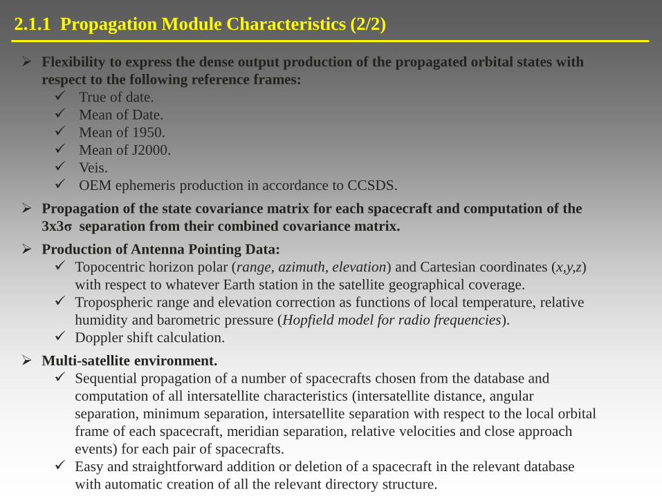
2.1.1 Propagation Module Characteristics (2/2)
Flexibility to express the dense output production of the propagated orbital states with
respect to the following reference frames:
True of date.
Mean of Date.
Mean of 1950.
Mean of J2000.
Veis.
OEM ephemeris production in accordance to CCSDS.
Propagation of the state covariance matrix for each spacecraft and computation of the
3x3σ separation from their combined covariance matrix.
Production of Antenna Pointing Data:
Topocentric horizon polar (range, azimuth, elevation) and Cartesian coordinates (x,y,z)
with respect to whatever Earth station in the satellite geographical coverage.
Tropospheric range and elevation correction as functions of local temperature, relative
humidity and barometric pressure (Hopfield model for radio frequencies).
Doppler shift calculation.
Multi-satellite environment.
Sequential propagation of a number of spacecrafts chosen from the database and
computation of all intersatellite characteristics (intersatellite distance, angular
separation, minimum separation, intersatellite separation with respect to the local orbital
frame of each spacecraft, meridian separation, relative velocities and close approach
events) for each pair of spacecrafts.
Easy and straightforward addition or deletion of a spacecraft in the relevant database
with automatic creation of all the relevant directory structure.
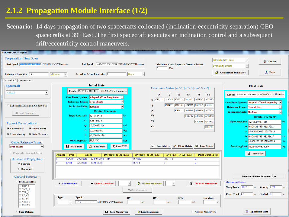
2.1.2 Propagation Module Interface (1/2)
Scenario: 14 days propagation of two spacecrafts collocated (inclination-eccentricity separation) GEO
spacecrafts at 39o East .The first spacecraft executes an inclination control and a subsequent
drift/eccentricity control maneuvers.
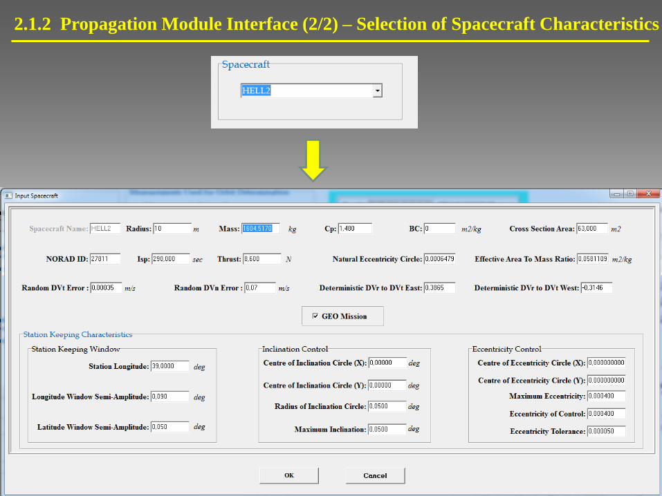
2.1.2 Propagation Module Interface (2/2) – Selection of Spacecraft Characteristics
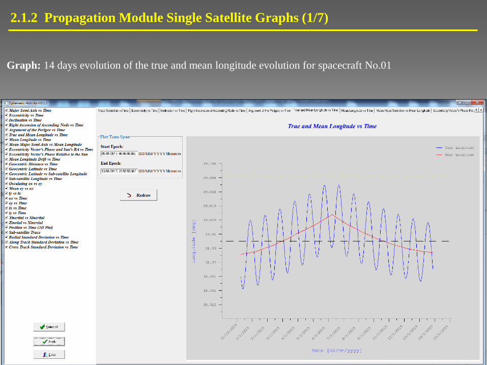
2.1.2 Propagation Module Single Satellite Graphs (1/7)
Graph: 14 days evolution of the true and mean longitude evolution for spacecraft No.01
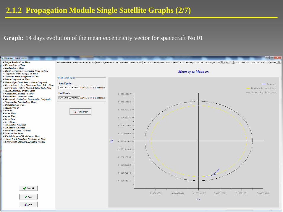
2.1.2 Propagation Module Single Satellite Graphs (2/7)
Graph: 14 days evolution of the mean eccentricity vector for spacecraft No.01

2.1.2 Propagation Module Single Satellite Graphs (3/7)
Graph: 14 days evolution of the inclination node vector for spacecraft No.01
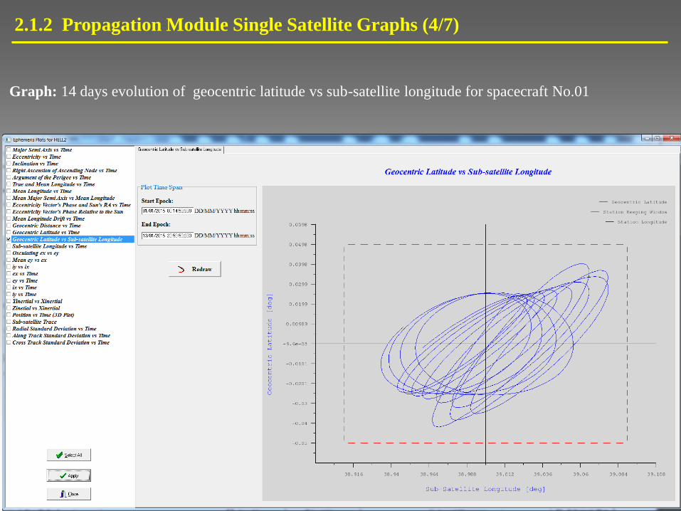
2.1.2 Propagation Module Single Satellite Graphs (4/7)
Graph: 14 days evolution of geocentric latitude vs sub-satellite longitude for spacecraft No.01
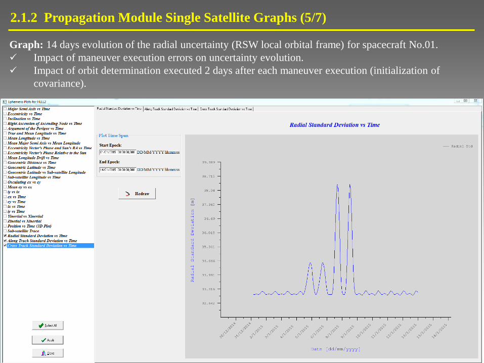
2.1.2 Propagation Module Single Satellite Graphs (5/7)
Graph: 14 days evolution of the radial uncertainty (RSW local orbital frame) for spacecraft No.01.
Impact of maneuver execution errors on uncertainty evolution.
Impact of orbit determination executed 2 days after each maneuver execution (initialization of
covariance).
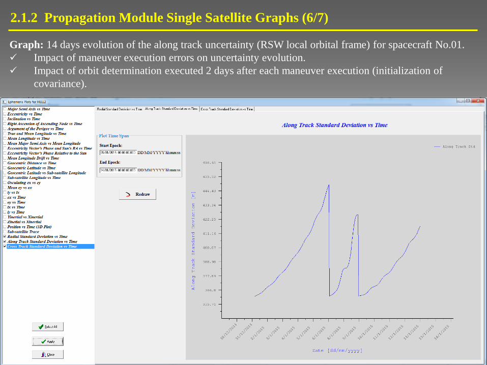
2.1.2 Propagation Module Single Satellite Graphs (6/7)
Graph: 14 days evolution of the along track uncertainty (RSW local orbital frame) for spacecraft No.01.
Impact of maneuver execution errors on uncertainty evolution.
Impact of orbit determination executed 2 days after each maneuver execution (initialization of
covariance).
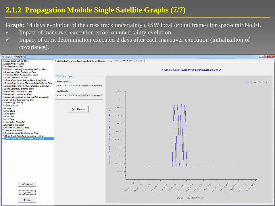
2.1.2 Propagation Module Single Satellite Graphs (7/7)
Graph: 14 days evolution of the cross track uncertainty (RSW local orbital frame) for spacecraft No.01.
Impact of maneuver execution errors on uncertainty evolution.
Impact of orbit determination executed 2 days after each maneuver execution (initialization of
covariance).

2.1.2 Propagation Module Double Satellite Graphs (1/6)
Graph: 14 days evolution of the sub-satellite longitude for both collocated spacecrafts.
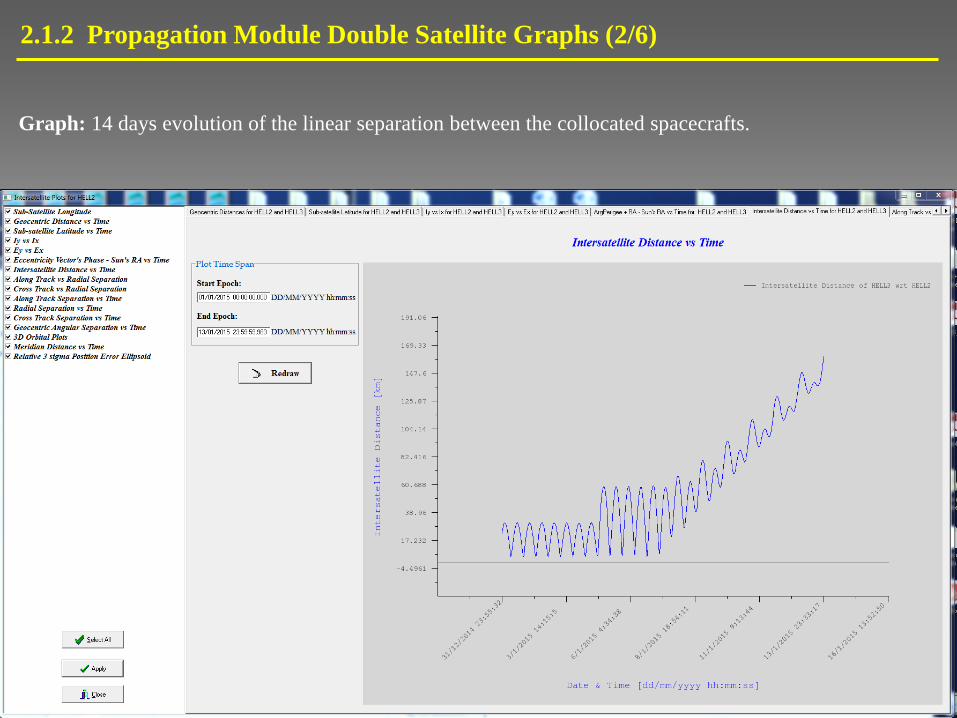
2.1.2 Propagation Module Double Satellite Graphs (2/6)
Graph: 14 days evolution of the linear separation between the collocated spacecrafts.
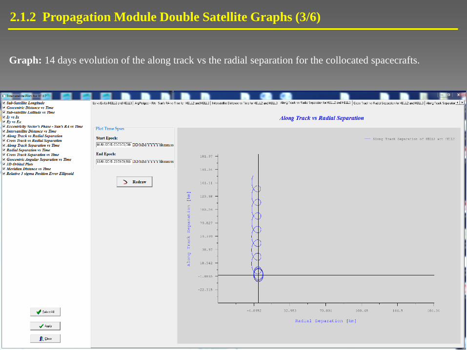
2.1.2 Propagation Module Double Satellite Graphs (3/6)
Graph: 14 days evolution of the along track vs the radial separation for the collocated spacecrafts.
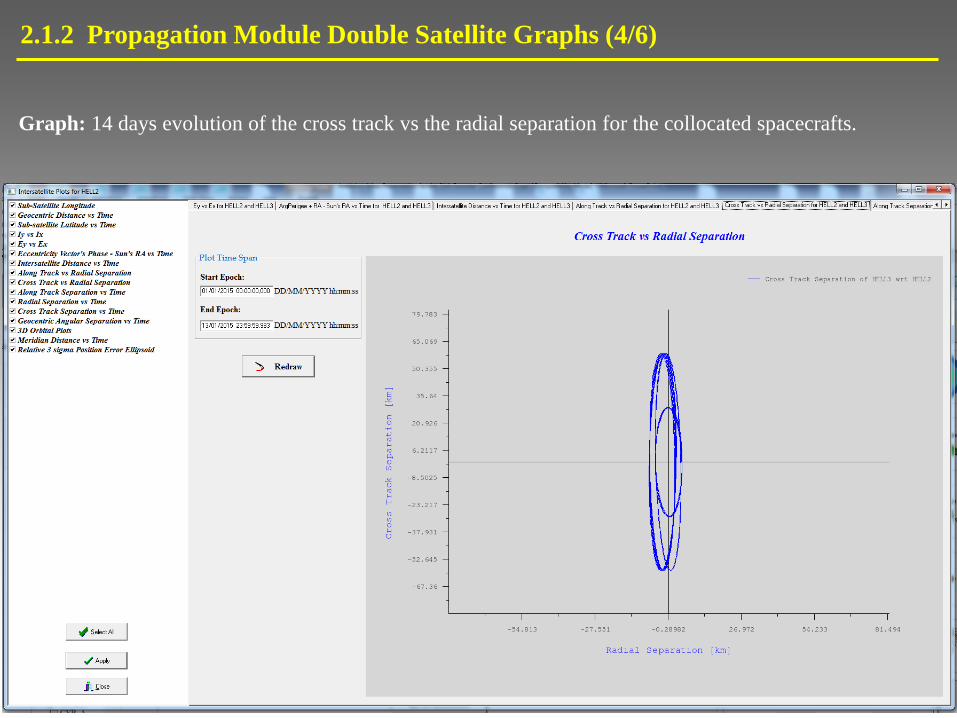
2.1.2 Propagation Module Double Satellite Graphs (4/6)
Graph: 14 days evolution of the cross track vs the radial separation for the collocated spacecrafts.
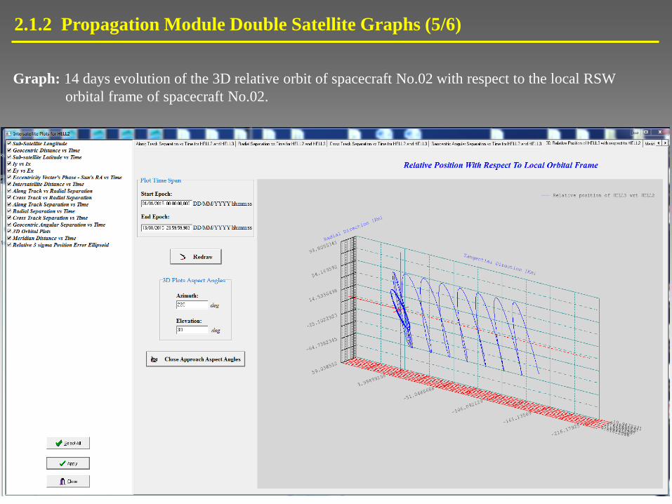
2.1.2 Propagation Module Double Satellite Graphs (5/6)
Graph: 14 days evolution of the 3D relative orbit of spacecraft No.02 with respect to the local RSW
orbital frame of spacecraft No.02.
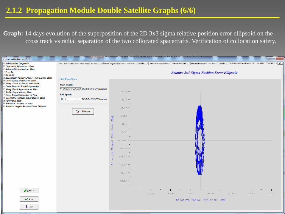
2.1.2 Propagation Module Double Satellite Graphs (6/6)
Graph: 14 days evolution of the superposition of the 2D 3x3 sigma relative position error ellipsoid on the
cross track vs radial separation of the two collocated spacecrafts. Verification of collocation safety.

Execution of an impulsive inclination control maneuver (South) followed by a continuous one (North).
Duration of continuous thrust maneuver : 3.47 hours
Maneuver acceleration of continuous thrust maneuver : 80 μm/s2
Spacecraft mass : 2000 Kgr
2.1.3 Mixing Continuous and Impulsive Thrust Maneuvers (1/2)

2.1.3 Mixing Continuous and Impulsive Thrust Maneuvers (2/2)
Graph: Evolution of inclination node vector under the impact of an impulsive inclination control
maneuver followed by a continuous inclination control maneuver.
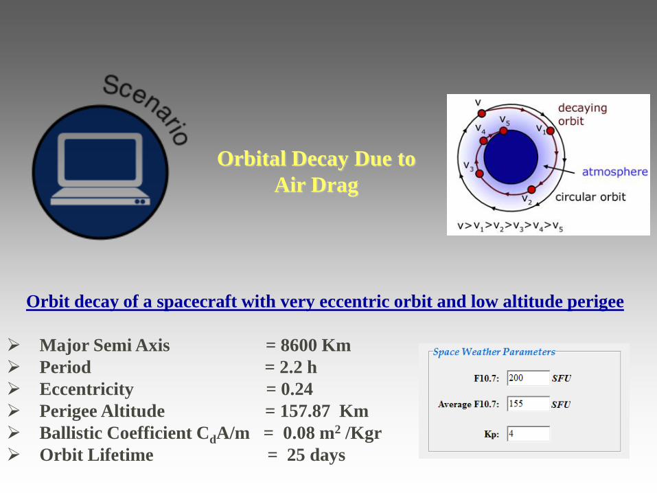
Orbit decay of a spacecraft with very eccentric orbit and low altitude perigee
Major Semi Axis = 8600 Km
Period = 2.2 h
Eccentricity = 0.24
Perigee Altitude = 157.87 Km
Ballistic Coefficient CdA/m = 0.08 m2 /Kgr
Orbit Lifetime = 25 days
Orbital Decay Due to
Air Drag
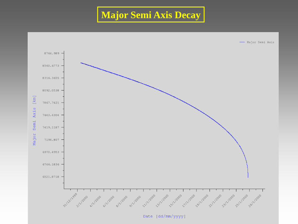
Major Semi Axis Decay
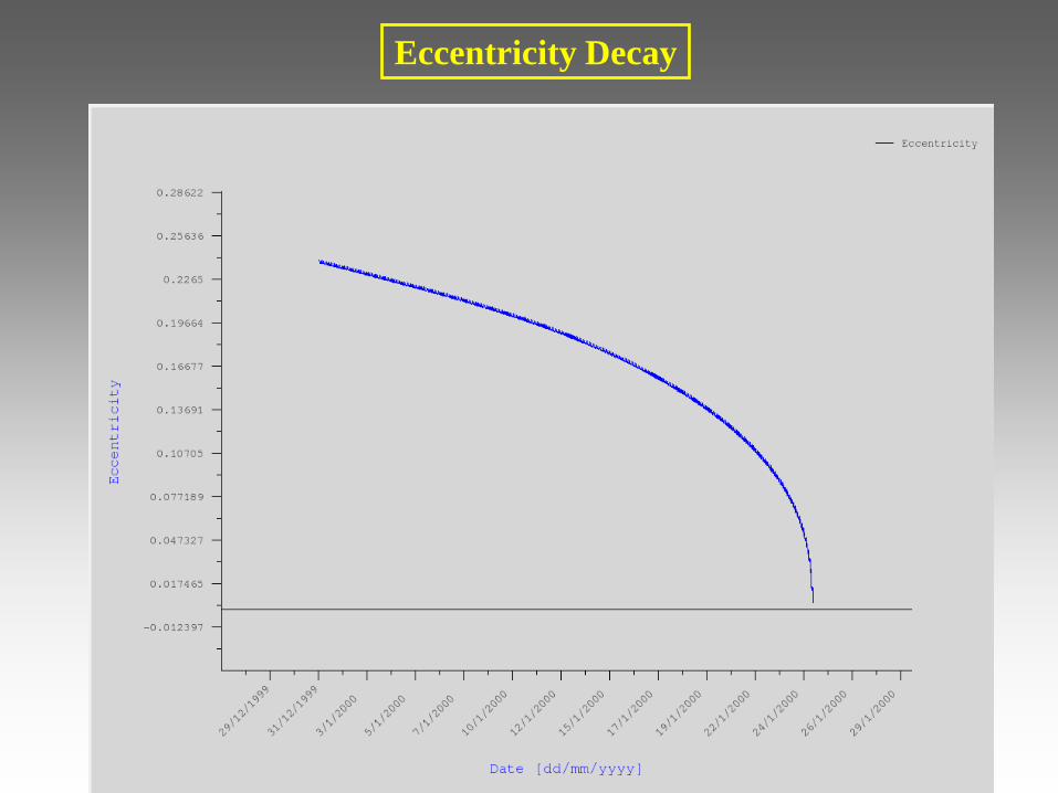
Eccentricity Decay

Geocentric Distance Decay

Y versus X Coordinate Referred to the True of Date Reference Frame
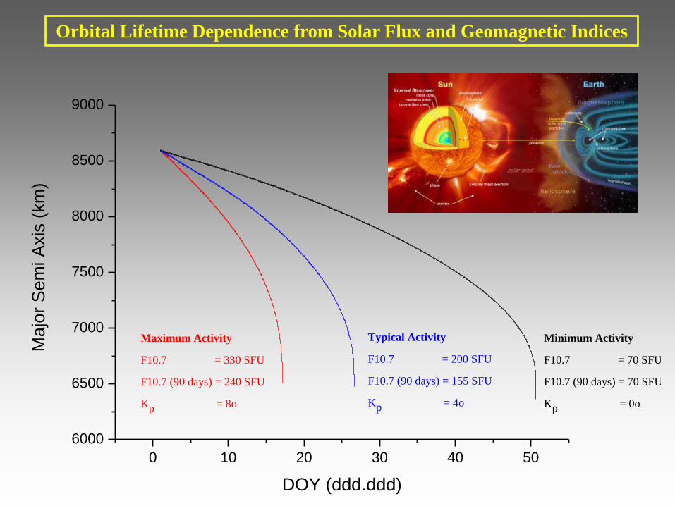
Orbital Lifetime Dependence from Solar Flux and Geomagnetic Indices
0 10 20 30 40 50
6000
6500
7000
7500
8000
8500
9000
Maximum Activity
F10.7 = 330 SFU
F10.7 (90 days) = 240 SFU
Kp = 8o
Typical Activity
F10.7 = 200 SFU
F10.7 (90 days) = 155 SFU
Kp = 4o
Majo
r S
em
i A
xis
(km
)
DOY (ddd.ddd)
Minimum Activity
F10.7 = 70 SFU
F10.7 (90 days) = 70 SFU
Kp = 0o
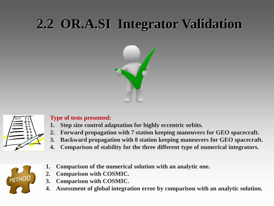
2.2 OR.A.SI Integrator Validation
Type of tests presented:
1. Step size control adaptation for highly eccentric orbits.
2. Forward propagation with 7 station keeping maneuvers for GEO spacecraft.
3. Backward propagation with 8 station keeping maneuvers for GEO spacecraft.
4. Comparison of stability for the three different type of numerical integrators.
1. Comparison of the numerical solution with an analytic one.
2. Comparison with COSMIC.
3. Comparison with COSMIC.
4. Assessment of global integration error by comparison with an analytic solution.
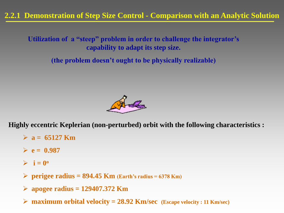
2.2.1 Demonstration of Step Size Control - Comparison with an Analytic Solution
Utilization of a “steep” problem in order to challenge the integrator’s
capability to adapt its step size.
(the problem doesn’t ought to be physically realizable)
Highly eccentric Keplerian (non-perturbed) orbit with the following characteristics :
a = 65127 Km
e = 0.987
i = 0o
perigee radius = 894.45 Km (Earth’s radius = 6378 Km)
apogee radius = 129407.372 Km
maximum orbital velocity = 28.92 Km/sec (Escape velocity : 11 Km/sec)
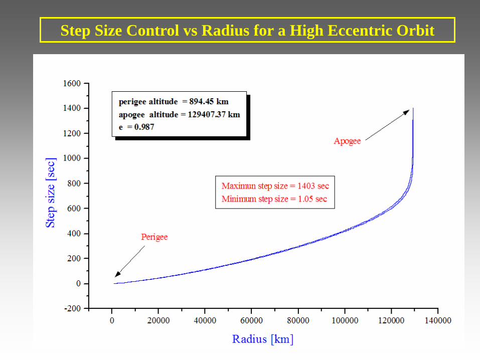
Step Size Control vs Radius for a High Eccentric Orbit

Relative Accuracy With Respect to the Analytic Solution
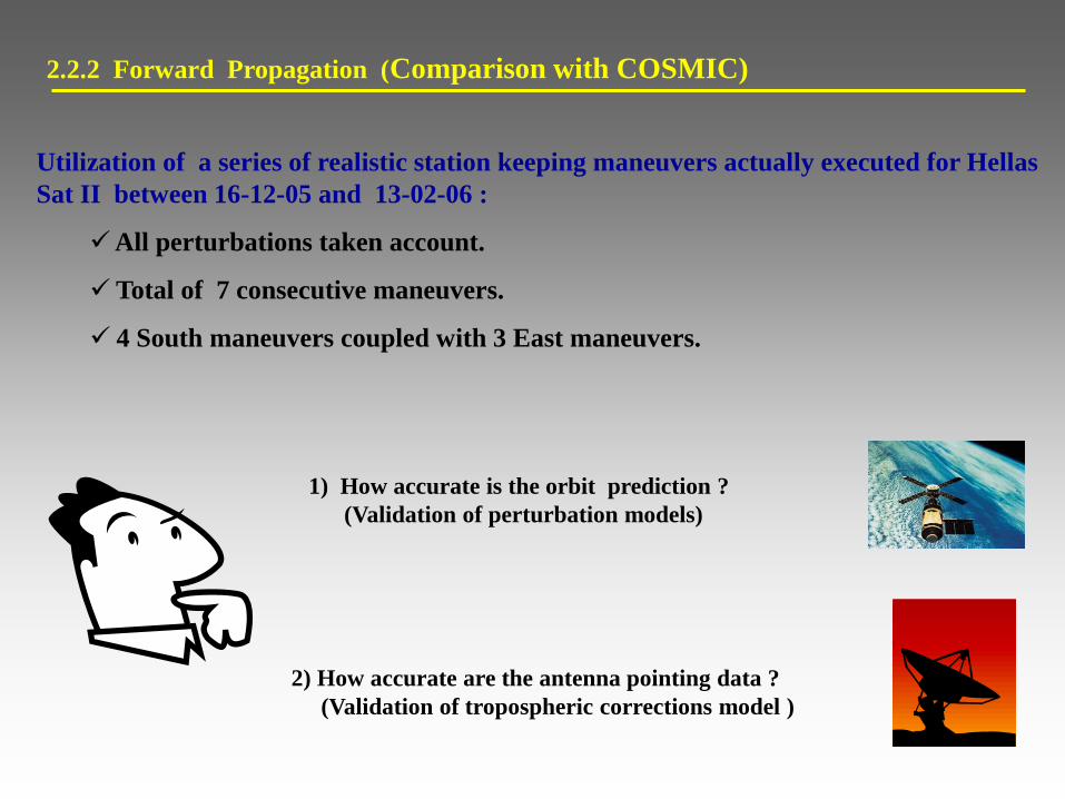
2.2.2 Forward Propagation (Comparison with COSMIC)
Utilization of a series of realistic station keeping maneuvers actually executed for Hellas
Sat II between 16-12-05 and 13-02-06 :
All perturbations taken account.
Total of 7 consecutive maneuvers.
4 South maneuvers coupled with 3 East maneuvers.
1) How accurate is the orbit prediction ?
(Validation of perturbation models)
2) How accurate are the antenna pointing data ?
(Validation of tropospheric corrections model )
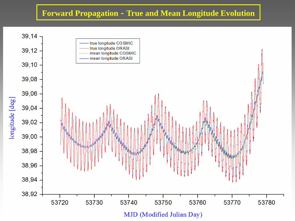
Forward Propagation - True and Mean Longitude Evolution
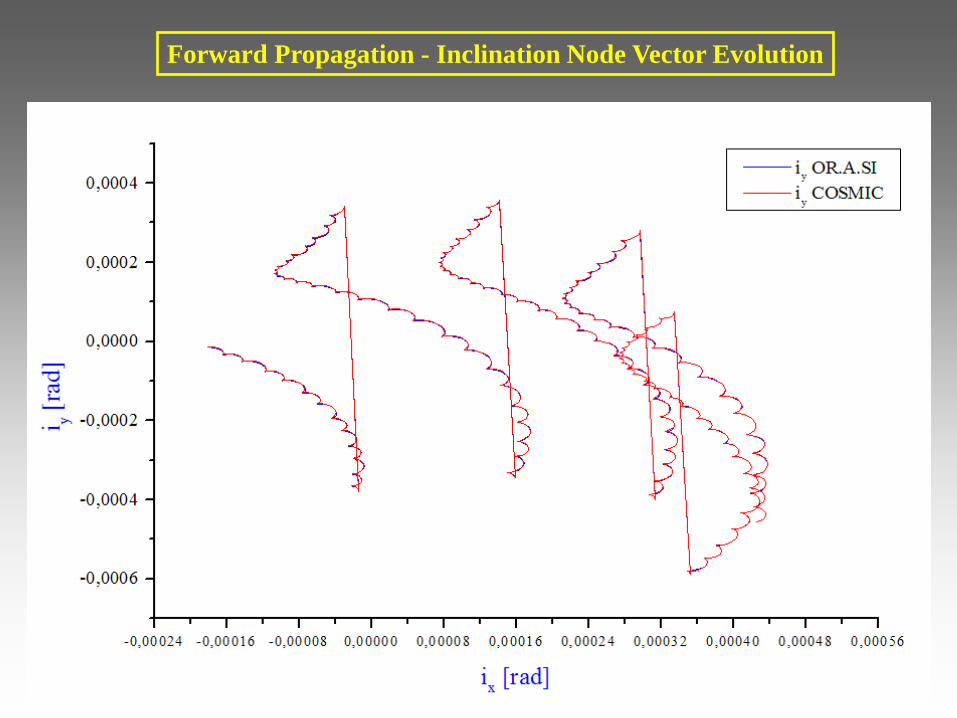
Forward Propagation - Inclination Node Vector Evolution
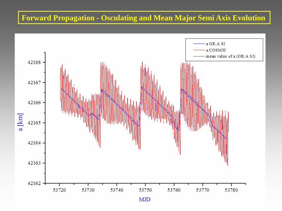
Forward Propagation - Osculating and Mean Major Semi Axis Evolution
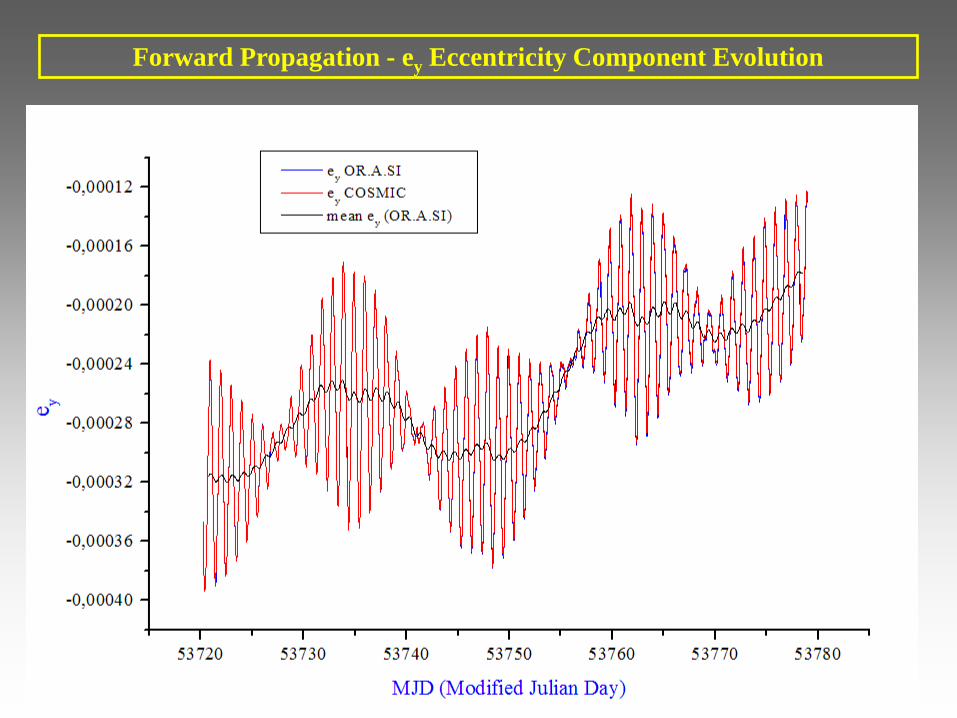
Forward Propagation - ey Eccentricity Component Evolution
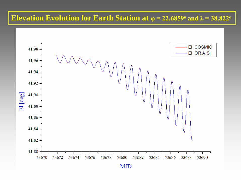
Elevation Evolution for Earth Station at φ = 22.6859ο and λ = 38.822ο

Azimuth Evolution for Earth Station at φ = 22.6859ο and λ = 38.822ο
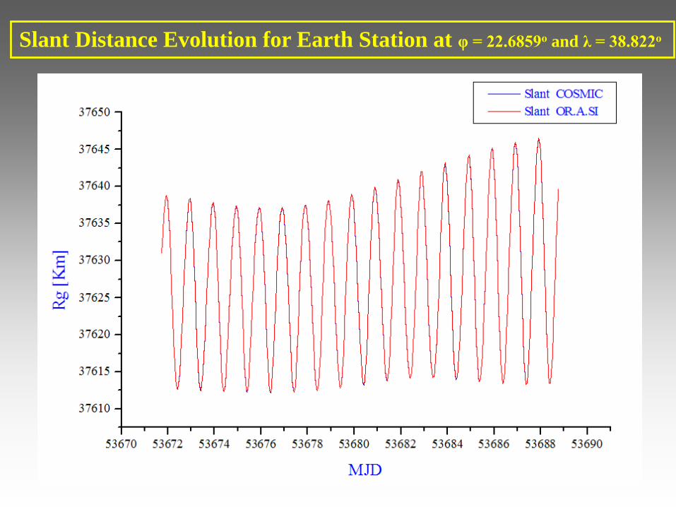
Slant Distance Evolution for Earth Station at φ = 22.6859ο and λ = 38.822ο
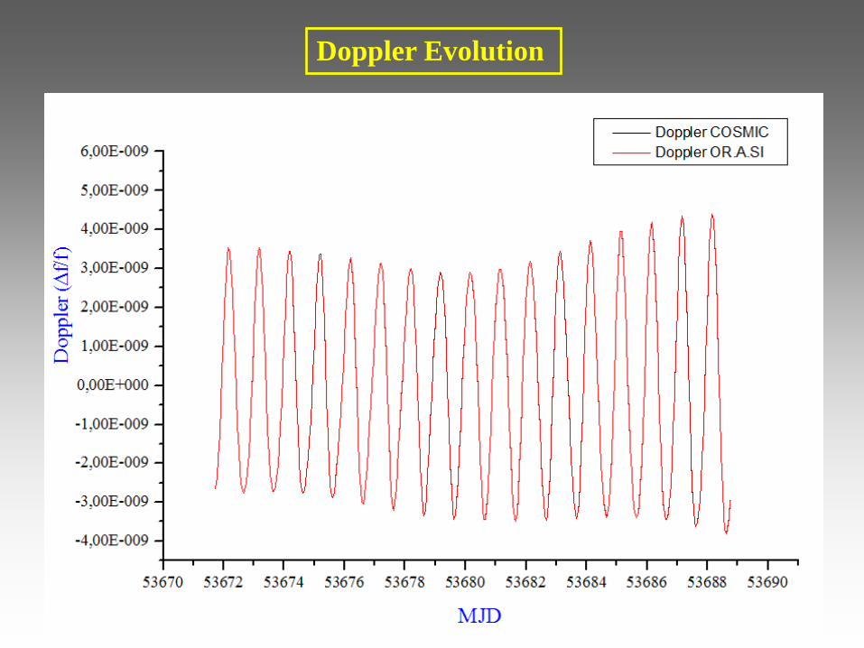
Doppler Evolution

2.2.3 Backward Propagation (Comparison with COSMIC)
Utilization of a series of realistic station keeping maneuvers actually executed for Hellas Sat II between
28-10-05 and 18-12-05 :
All perturbations taken account.
Total of 8 consecutive maneuvers.
4 South maneuvers coupled with 3 East maneuvers and a West one.
Backward evolution of inertial coordinate differences between COSMIC and OR.A.SI

Backward Propagation with 8 Maneuvers – True Longitude Evolution

Backward Propagation with 8 Maneuvers – Inclination Node Vector Evolution
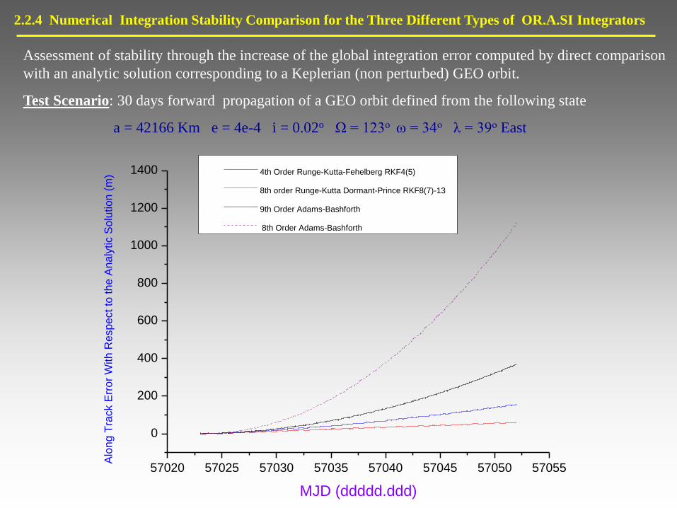
2.2.4 Numerical Integration Stability Comparison for the Three Different Types of OR.A.SI Integrators
Assessment of stability through the increase of the global integration error computed by direct comparison
with an analytic solution corresponding to a Keplerian (non perturbed) GEO orbit.
Test Scenario: 30 days forward propagation of a GEO orbit defined from the following state
a = 42166 Km e = 4e-4 i = 0.02o Ω = 123ο ω = 34ο λ = 39ο East
57020 57025 57030 57035 57040 57045 57050 57055
0
200
400
600
800
1000
1200
1400
Alo
ng
Tra
ck E
rro
r W
ith
Re
sp
ect
to t
he
An
aly
tic S
olu
tio
n (
m)
MJD (ddddd.ddd)
4th Order Runge-Kutta-Fehelberg RKF4(5)
8th order Runge-Kutta Dormant-Prince RKF8(7)-13
9th Order Adams-Bashforth
8th Order Adams-Bashforth

3.1 Station Keeping
Maneuver Computation
for GEO Spacecrafts
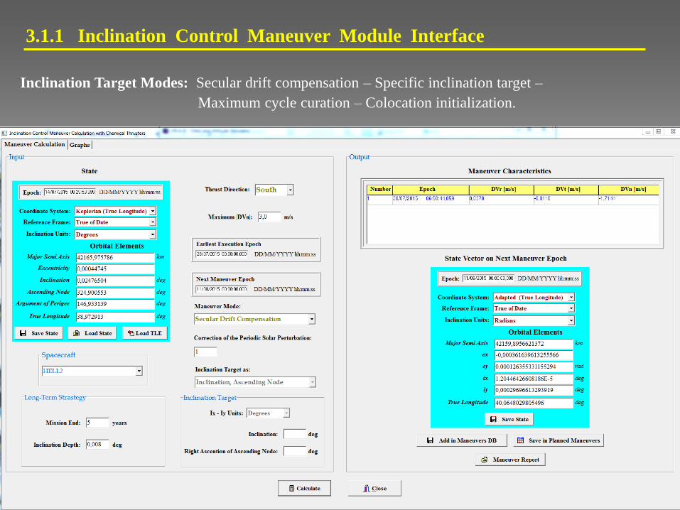
3.1.1 Inclination Control Maneuver Module Interface
Inclination Target Modes: Secular drift compensation – Specific inclination target –
Maximum cycle curation – Colocation initialization.
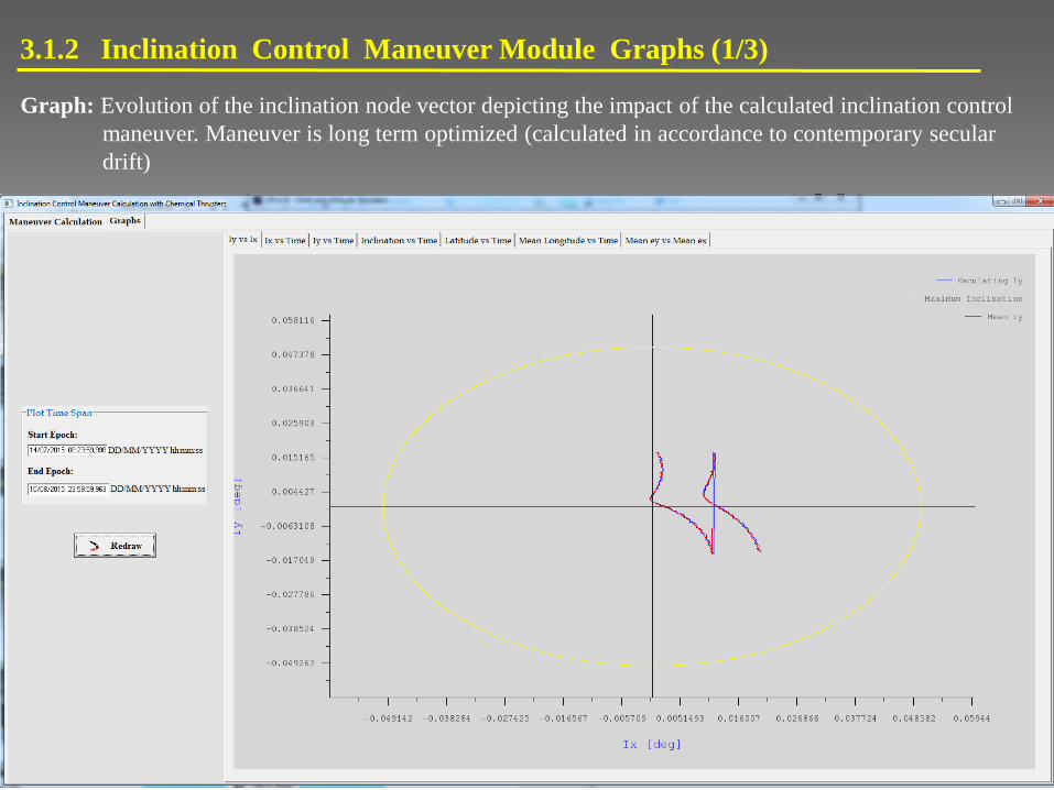
3.1.2 Inclination Control Maneuver Module Graphs (1/3)
Graph: Evolution of the inclination node vector depicting the impact of the calculated inclination control
maneuver. Maneuver is long term optimized (calculated in accordance to contemporary secular
drift)
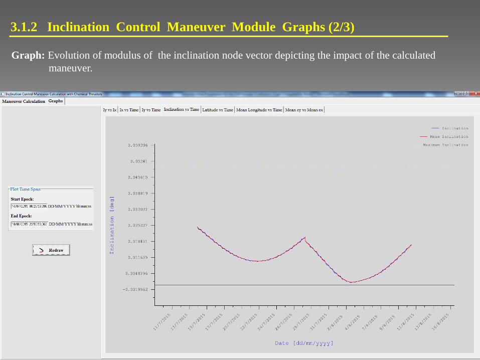
3.1.2 Inclination Control Maneuver Module Graphs (2/3)
Graph: Evolution of modulus of the inclination node vector depicting the impact of the calculated
maneuver.
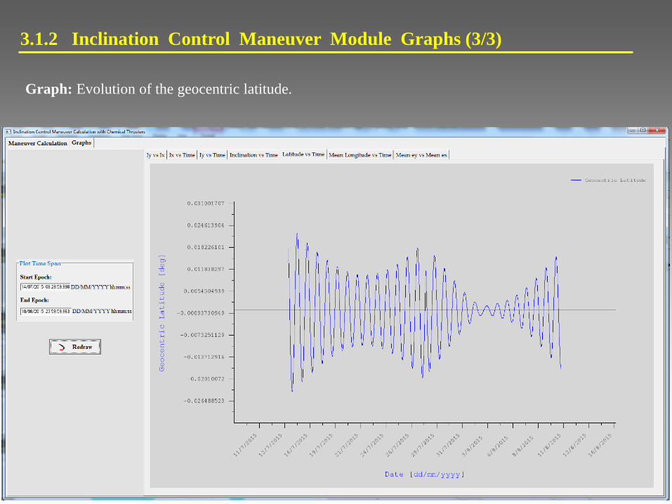
3.1.2 Inclination Control Maneuver Module Graphs (3/3)
Graph: Evolution of the geocentric latitude.
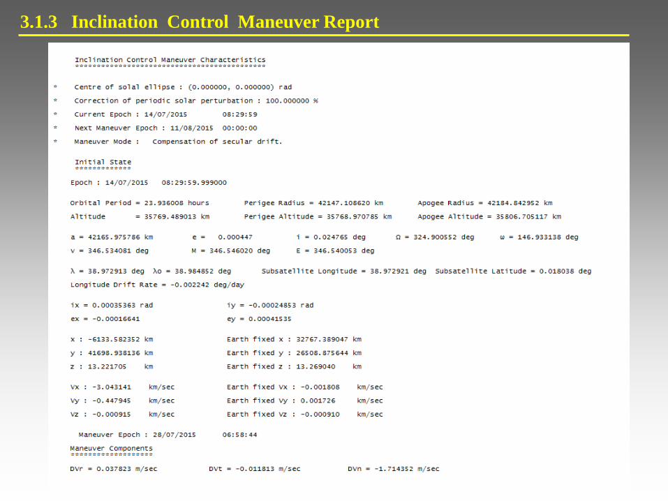
3.1.3 Inclination Control Maneuver Report
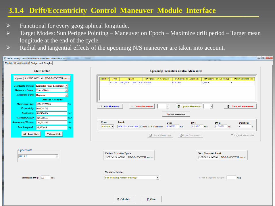
3.1.4 Drift/Eccentricity Control Maneuver Module Interface
Functional for every geographical longitude.
Target Modes: Sun Perigee Pointing – Maneuver on Epoch – Maximize drift period – Target mean
longitude at the end of the cycle.
Radial and tangential effects of the upcoming N/S maneuver are taken into account.

3.1.5 Drift/Eccentricity Control Maneuver Module Graphs (1/5)
Graph: Evolution of the mean and true longitude depicting the impact of the calculated drift/eccentricity
control maneuver as well as the impact of the triaxiality of the upcoming inclination control
maneuver.
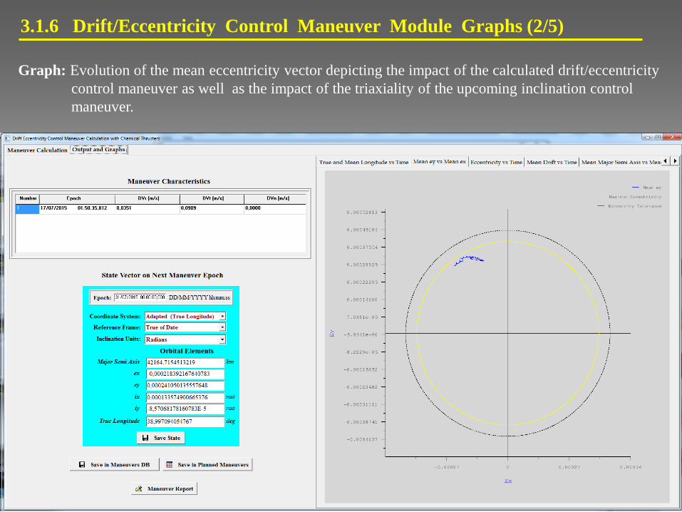
3.1.6 Drift/Eccentricity Control Maneuver Module Graphs (2/5)
Graph: Evolution of the mean eccentricity vector depicting the impact of the calculated drift/eccentricity
control maneuver as well as the impact of the triaxiality of the upcoming inclination control
maneuver.
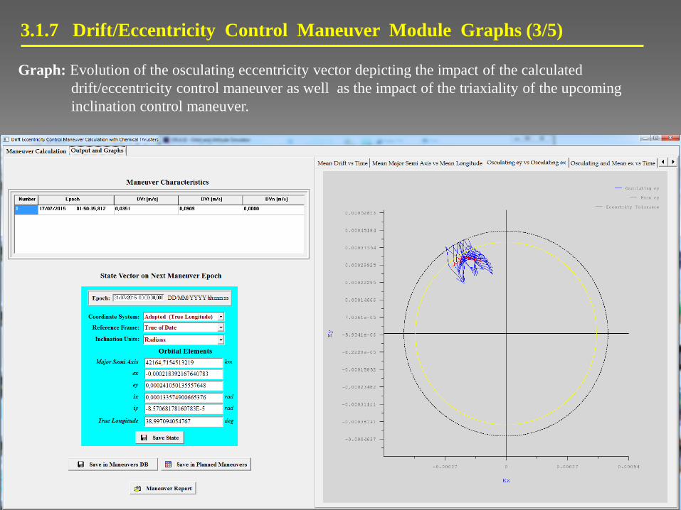
3.1.7 Drift/Eccentricity Control Maneuver Module Graphs (3/5)
Graph: Evolution of the osculating eccentricity vector depicting the impact of the calculated
drift/eccentricity control maneuver as well as the impact of the triaxiality of the upcoming
inclination control maneuver.

3.1.8 Drift/Eccentricity Control Maneuver Module Graphs (4/5)
Graph: Evolution of the mean longitude drift depicting the impact of the calculated drift/eccentricity
control maneuver as well as the impact of the triaxiality of the upcoming inclination control
maneuver.

3.1.9 Drift/Eccentricity Control Maneuver Module Graphs (5/5)
Graph: Mean major semi axis vs mean longitude depicting the impact of the calculated drift/eccentricity
control maneuver as well as the impact of the triaxiality of the upcoming inclination control
maneuver.

3.1.10 Drift/Eccentricity Control Maneuver Report
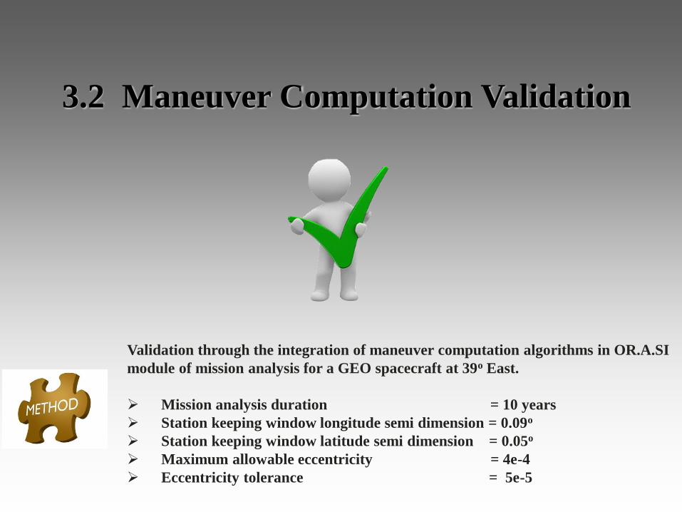
3.2 Maneuver Computation Validation
Validation through the integration of maneuver computation algorithms in OR.A.SI
module of mission analysis for a GEO spacecraft at 39o East.
Mission analysis duration = 10 years
Station keeping window longitude semi dimension = 0.09o
Station keeping window latitude semi dimension = 0.05o
Maximum allowable eccentricity = 4e-4
Eccentricity tolerance = 5e-5

3.2.1 Inclination Control Maneuvers
Inclination node vector evolution Inclination modulus evolution
Latitude vs longitude evolution Latitude evolution

3.2.1 Drift/Eccentricity Control Maneuvers
Mean eccentricity vector evolution Eccentricity modulus evolution
True longitude evolution Ω+ω evolution

4.1 Maneuver Restitution
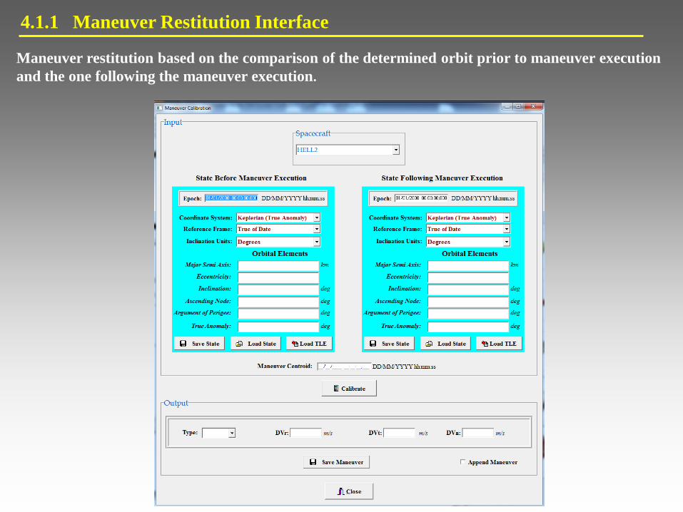
4.1.1 Maneuver Restitution Interface
Maneuver restitution based on the comparison of the determined orbit prior to maneuver execution
and the one following the maneuver execution.

4.2 Maneuver Restitution Validation
Comparison with actual inclination control maneuver restitution done with focusGEO
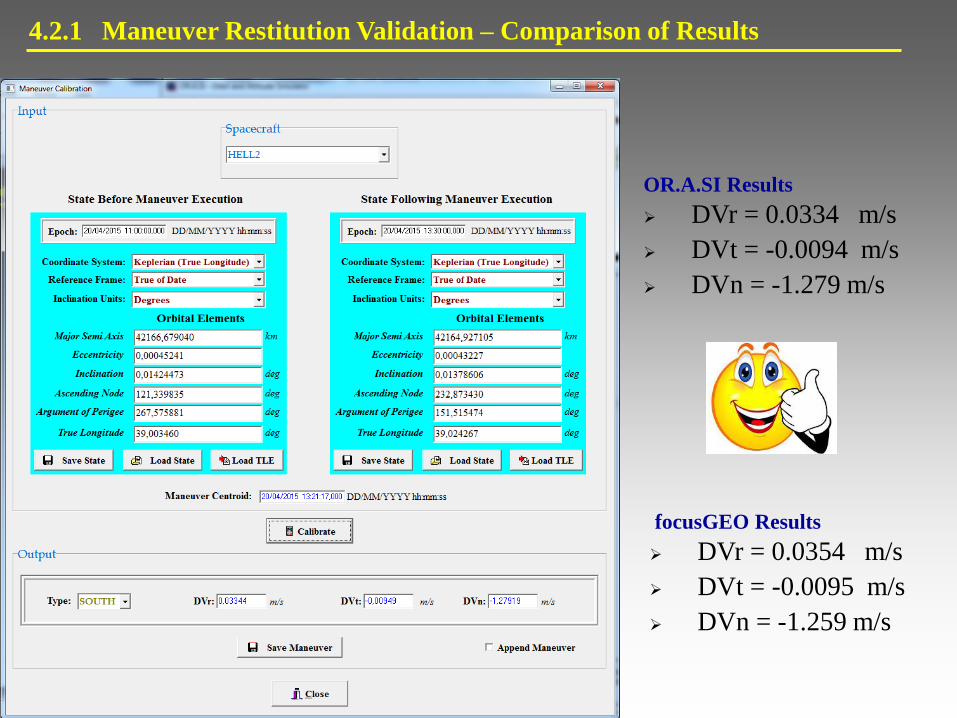
4.2.1 Maneuver Restitution Validation – Comparison of Results
OR.A.SI Results
DVr = 0.0334 m/s
DVt = -0.0094 m/s
DVn = -1.279 m/s
focusGEO Results
DVr = 0.0354 m/s
DVt = -0.0095 m/s
DVn = -1.259 m/s
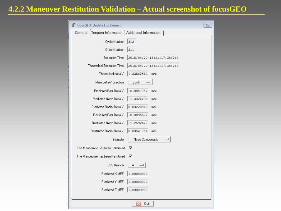
4.2.2 Maneuver Restitution Validation – Actual screenshot of focusGEO

5. Relocation Maneuvers Module
for GEO Spacecrafts
(Only in console GUI. Pending to be implemented in windows GUI)
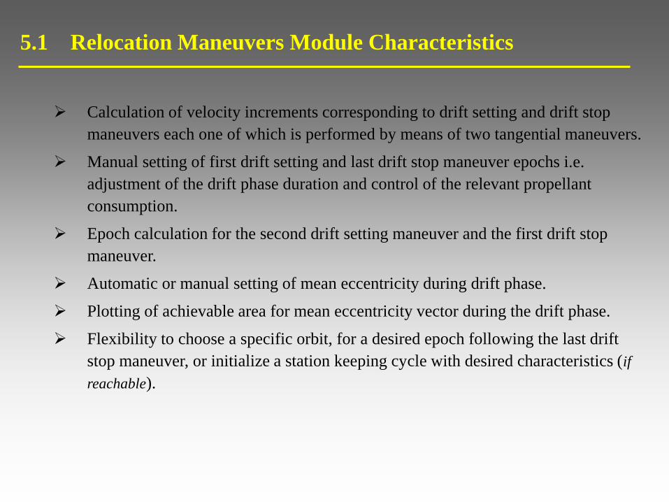
5.1 Relocation Maneuvers Module Characteristics
Calculation of velocity increments corresponding to drift setting and drift stop
maneuvers each one of which is performed by means of two tangential maneuvers.
Manual setting of first drift setting and last drift stop maneuver epochs i.e.
adjustment of the drift phase duration and control of the relevant propellant
consumption.
Epoch calculation for the second drift setting maneuver and the first drift stop
maneuver.
Automatic or manual setting of mean eccentricity during drift phase.
Plotting of achievable area for mean eccentricity vector during the drift phase.
Flexibility to choose a specific orbit, for a desired epoch following the last drift
stop maneuver, or initialize a station keeping cycle with desired characteristics (if
reachable).

Relocation from 39o East to 42o East and Initialization of a 14 day Station Keeping Cycle
Input
Initial State : a = 42166.0 Km ex = -0.0002 ey = 0 lo = 39o East
State Epoch : 01/03/2010 00:00:00 UTC
Target State : Initialization of a 14 day station keeping cycle at 42o East
Eccentricity of Control : 0.00035 [Centre of eccentricity circle is (0,0)]
Target Epoch : 28/03/2010 00:00:00 UTC
First Drift Setting Maneuver Epoch : 04/03/2010 00:00:00 UTC
Last Drift Stop Maneuver Epoch : 24/03/2010 00:00:00 UTC (20 days of drift)
Output
First Drift Setting Maneuver : DV1 = -0.262844m/s
Second Drift Setting Maneuver : DV2 = -0.109244m/s
Second Drift Setting Maneuver Epoch : 04/03/10 19:51:48 UTC
First Drift Stop Maneuver : DV3 = 0.469886 m/s
First Drift Stop Maneuver Epoch : 23/03/2010 08:29:39 UTC
Last Drift Stop Maneuver : DV4 = 0.87668 m/s

Relocation from 39o East to 42o East – Longitude Evolution
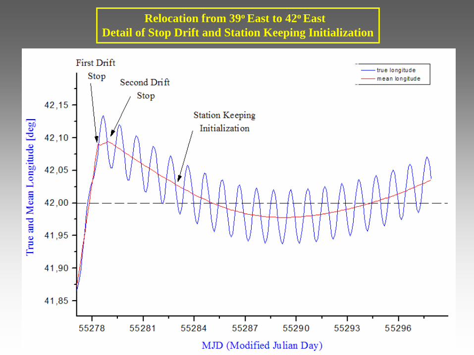
Relocation from 39o East to 42o East
Detail of Stop Drift and Station Keeping Initialization
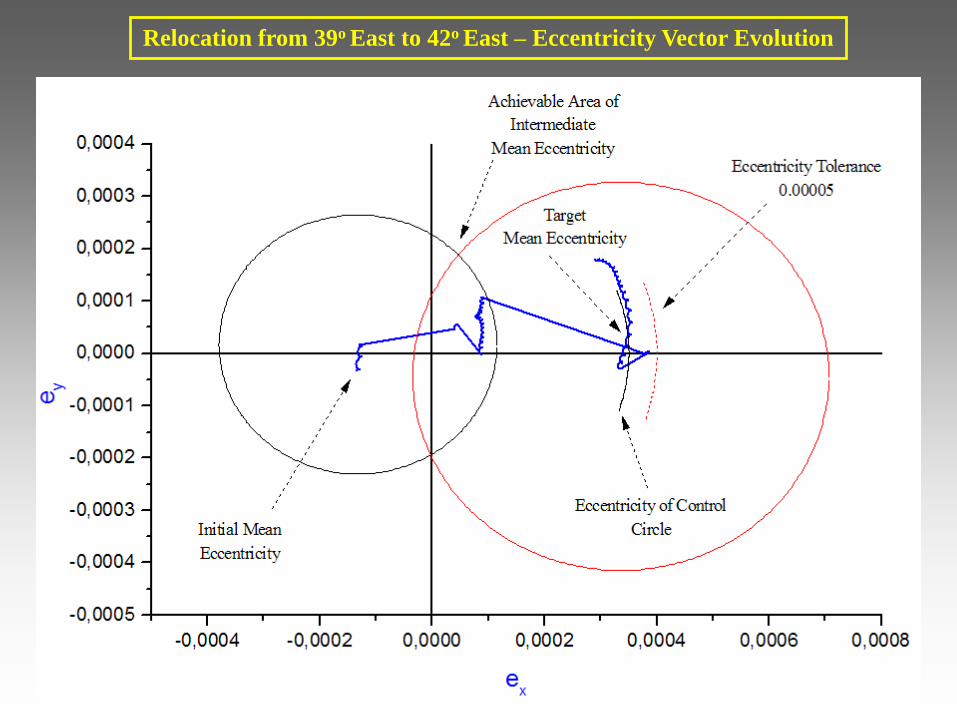
Relocation from 39o East to 42o East – Eccentricity Vector Evolution
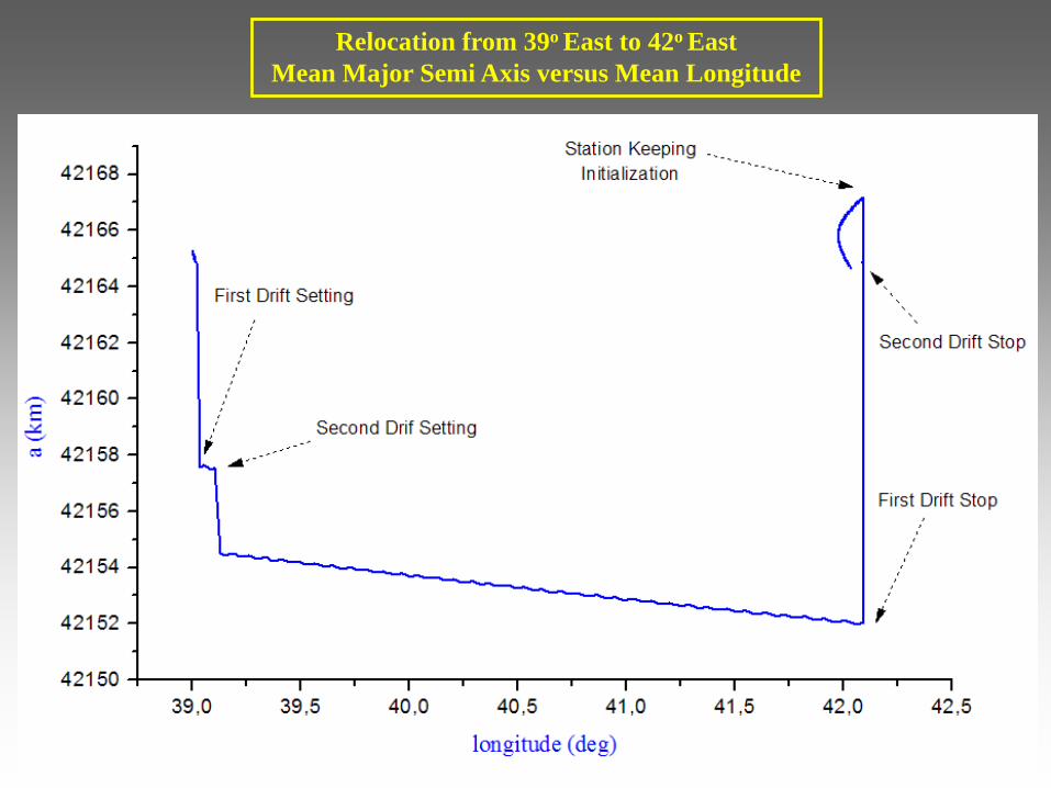
Relocation from 39o East to 42o East
Mean Major Semi Axis versus Mean Longitude


