Flight Testing in a Simulation Based Environment

American Institute of Aeronautics and Astronautics

1

Flight Testing in a Simulation Based Environment David W. Babka

1

California Polytechnic University, San Luis Obispo, CA, 93405

1 Undergraduate, Aerospace Engineering, 1 Grande Ave, San Luis Obispo CA 93407, AIAA Member 437959


2

Abstract

Over the past two decades performance flight testing of full scale aircraft has transferred

some of the testing workload to simulation based systems. Flight testing full scale aircraft in

the real world environment has always been expensive, especially now with the rise in

aviation fuel costs. Additionally, new emerging technologies require extensive testing and

doing so in the full scale environment is cost prohibitive. A cheaper alternative is to test

systems in a simulation based environment. Not only can aircraft be simulated via a

computer, but all the aircrafts systems can be modeled in the simulation. Furthermore, most

of the aircraft systems, such as avionics and sensors, can be directly built into the simulation

just as they would be on the actual aircraft. The purpose of this report is to review the

progression of flight simulation technology, flight testing procedures, and conduct a series of

flight tests to compare the data between the actual aircraft in flight with two simulators

readily available to the general public. The two simulators considered are X-Plane 9 by

Laminar Research and Flight Simulator X from Microsoft. Each simulator uses a different

approach to creating the simulated environment. X-Plane uses an engineering process called

“Blade Element Theory”, while Microsoft Flight Simulator X uses the more traditional

stability derivative method. In order to compare the accuracy of each of these simulations,

three flight tests were conducted in each simulator and in the actual aircraft. A Cessna

172SP was the aircraft used in each of the tests. The three tests conducted were flight path

stability, stall, and steady turns. Comparing the results, the simulations produced data very

similar to that of the actual tests; however, the data did not suggest that either simulation

was more accurate than the other. The only distinction between the two simulators that

could be made was evident in their user interfaces and ease of operation. Overall, the results

obtained in this paper illustrate the effectiveness of the modern flight simulator as an

effective testing and design tool.

Acknowledgements

First, I would like to thank Dr. William Durgin for his guidance during the course of the project. Additionally, the

flight tests in the actual aircraft could not have taken place if it were not for the efforts of Jeannine and Gary Sparks

at the Pacific Aerocademy. The test aircraft, N172CY, was always in top condition and ready to complete the flight

tests without any maintenance related issues.


3

Table of Contents

Abstract.......................................................................................................................................................................... 2 Acknowledgements ....................................................................................................................................................... 2 Table of Contents........................................................................................................................................................... 3 List of Figures ................................................................................................................................................................ 3 List of Tables ................................................................................................................................................................. 3 I. Introduction ........................................................................................................................................................... 4 II. Literature Review ................................................................................................................................................. 5

A. NASA HiMAT Vehicle Simulation.................................................................................................................. 5 B. Integration of Open Source Flight Simulation Software in Testing UAVs ...................................................... 6

III. Methodology and Results ................................................................................................................................. 7 A. Safety ................................................................................................................................................................ 8 B. Data Acquisition ............................................................................................................................................... 9 C. Test Procedure – Stalls ................................................................................................................................... 10 D. Test Procedure – Steady Turn ........................................................................................................................ 11 E. Test Procedure – Flight Path Stability ............................................................................................................ 12 F. Results – Stall ................................................................................................................................................. 12 G. Results – Steady Turn ..................................................................................................................................... 13 H. Results – Flight Path Stability ........................................................................................................................ 14 I. Flight Simulator GPS Data ............................................................................................................................. 15

IV. Conclusion ...................................................................................................................................................... 16 V. Appendix ............................................................................................................................................................. 17 References ................................................................................................................................................................... 18

List of Figures

Figure 1. Lockheed Martin's commercial flight simulator: Prepar3D ........................................................................... 4 Figure 2. The HiMAT three-view reveals its special characteristics. ............................................................................ 5 Figure 3. The Basic simulation was compact and simple. ............................................................................................. 6 Figure 4. FlightGear/JSBSim and MATLAB/Simulink were used together to model the UAV's flight model and

autopilot respectively6. .................................................................................................................................................. 6

Figure 5. X-Plane performs multiple calculations per second to determine how the aircraft actually flies. .................. 7 Figure 6. FSX uses stability derivatives to predict how the aircraft should fly. ............................................................ 7 Figure 7. MIL-STD-882B Hazard matrix helps prevent accidents. .............................................................................. 8 Figure 8. The Go Pro

® HD video camera was invaluable in acquiring the required test data. ..................................... 9

Figure 9. FS Recorder allows for a multitude of aircraft data to be recorded. ............................................................... 9 Figure 10. X-Plane boasts an extensive data recording capability. .............................................................................. 10 Figure 11. FSX and X-Plane have the ability to customize the weight and balance of the aircraft. ............................ 11 Figure 12. Power on stall test results ........................................................................................................................... 12 Figure 13. Power off stall test results .......................................................................................................................... 13 Figure 14. Steady turn test results ................................................................................................................................ 14 Figure 15. Flight path stability test with flaps deployed .............................................................................................. 15 Figure 16. Flight path stability test without flaps ........................................................................................................ 15 Figure 17. X-Plane GPS track data .............................................................................................................................. 17 Figure 18. FSX GPS track data .................................................................................................................................... 17

List of Tables

Table 1. Flight testing has some critical hazards. .......................................................................................................... 8 Table 2. FSX data output sample ................................................................................................................................. 18 Table 3. X-Plane data output sample ........................................................................................................................... 18


4

Figure 1. Lockheed Martin's commercial flight simulator: Prepar3D

I. Introduction

IRCRAFT flight testing is one of the most costly but essential steps in the design and manufacturing process.

Before any aircraft, whether it be for the military or civilian markets, is ready for deployment, they must

undergo a rigorous series of flight tests. Furthermore, flight testing programs are developed with the goal of

revealing design flaws and providing necessary data for certification1. Before the age of computers, all flight tests

were conducted on the prototype aircraft; consequently, design flaws which led to aircraft damage proved to be

extremely expensive and would stop the design process until the prototype could be fixed and redesigned. The

modern computer and the development of simulation based flight testing changed the design process completely.

Once computer technology caught up with the aerospace industry, the potential for aircraft design and testing

became limitless. Aircraft developers were enabled to design, model, and test their aircraft in a safe and cost

effective manner. Instead of having to repair a damaged airframe after a mishap in preliminary testing, the designer

could simply make the design change in the computer model and re-fly the test. Additionally, simulation based

testing helped reduce the cost of the testing process because simulators don’t require fuel like their real world

counterparts. The cost of fuel is one of the biggest limiting factors to flight testing. When a test program is

developed, a specific amount of tests are planned in order to meet all the testing requirements and minimize the cost

of the program. Because many designers outsource the flight testing process to a 3rd

party, the testing agency incurs

all additional expenses in the event a test requires repeating. Moreover, it would be more cost effective to test the

aircraft model in a simulated environment first to reveal any design flaws beforehand.

With the ever rising price of oil, the use of simulation based flight testing is becoming more widely used as a

primary means for testing. Both civilian and military programs have contributed to the development of the

sophisticated simulators seen today. Most notably, Microsoft’s flight simulation software, Microsoft ESP, was

purchased by Lockheed Martin which

used the technology to create a

versatile simulation tool for

preliminary testing. Lockheed’s

resulting software is called Prepar3D

and has been packaged to sell to the

commercial market. Figure 1 shows a

rendering of the visual environment

which Prepar3D creates3. A result

from the development of high-tech

simulators was the creation of medium

fidelity consumer applications. The

simulations that were developed for the

consumer allowed the general public to

experience the same simulation

technologies used in commercial

applications for recreational and

educational purposes. The widespread

use of the cheap, home-based flight

simulators spawned a large community

of flight simulator enthusiasts.

Furthermore, the continued development of the home-based simulator has resulted in cheap and accurate simulation

tools which have the potential to be used with a multitude of applications.

The following paper explores the flight testing capabilities of home-based flight simulation models and

environments. Primarily, the home-based simulator is designed for entertainment purposes; however, the

educational applications are limitless. In order to demonstrate the capabilities of the home-based simulator, baseline

tests were first conducted in an actual Cessna 172SP in the San Luis Obispo County area. The tests were then

repeated in two different simulations and the data from all three tests were compared. Similar data sets would reveal

the usefulness of the home-based simulators for educational and practical applications. In addition to investigating

A


5

the usefulness of the home-based simulator, the overall project provided a great opportunity to learn flight testing

protocols and flying techniques as well as an opportunity to develop data reduction scripts in MATLAB.

II. Literature Review

As the requirements for aerospace vehicles have become more advanced and exotic, the need for accurate, high-

tech simulation software has increased accordingly. The new advanced aerospace systems are expensive to test full

scale, thus developers must rely on scaled tests and simulations for preliminary testing. Finding design flaws at the

early stages of design is vital in producing a product quickly and cost effectively.

In addition to being an invaluable tool to larger aerospace applications, less sophisticated simulation

environments have extremely important applications for smaller, private designs and education opportunities. Home

build aircraft designers can save themselves hours of troubleshooting and development costs by using cheap but

effective simulations for their preliminary testing needs.

The following literature reviews will discuss simulation software which has been used for advanced aerospace

concepts, as well as software that is currently being used presently. The first paper discusses the role of simulation

in the development and flight testing of Highly Maneuverable Aircraft Technology (HiMAT) written by NASA

engineers. Figure 2 illustrates the HiMAT concept via a three view drawing. Second, a paper was reviewed which

discussed the use of open source, or free, software to simulate the testing of an autonomous unmanned aerial vehicle

(UAV).

A. NASA HiMAT Vehicle Simulation

Beginning in the early 1980’s,

NASA began realizing the potential for

the use of high fidelity simulation

software. Full scale tests had become

extremely expensive and in some cases

impossible to perform. When studying

the HiMAT vehicle concept, NASA

engineers showed that flight simulation

was “the key to flight qualification of

the HiMAT vehicle.”1 The HiMAT

vehicle concept was designed to

demonstrate the maneuvering

capabilities of an aircraft with reduced

static stability and digital fly-by-wire

controls. Because the HiMAT program

planned for a “limited amount of

flights” and had an “unstable aircraft configuration”, simulations were “essential to the HiMAT program.” During

the course of the HiMAT program many different simulation modules were developed. Some of the key

components to note are the aerodynamics, primary and secondary control, propulsion, and uplink and downlink

models. Each module closely simulates their actual real world counterparts and allowed the designers the chance to

correct issues before actual tests were conducted. For instance, when simulating the downlink system, the designers

were able to solve issues while still in the simulation.

Four different simulation versions were developed for the HiMAT vehicle: the Basic, Verification, computation

and simulation of HiMAT (CASH), and Iron Bird. The Basic simulation was the most widely used because it

allowed for “relative ease of program modification” and the use of the “fewest number of computers”. Ultimately,

the basic simulation “provided the principle tool for the final design”. Figure 3 shows the actual Basic simulation

block diagram used in the HiMAT program.

The next evolution to the simulation environment was the Verification simulator, which had the primary purpose

of verifying the flight code and making sure the systems perform exactly as specified. Because most of the codes

used in the simulation are those actually used on the aircraft, the must be verified in the simulator before being

implanted practically.

The third type of simulation performed was the CASH simulation. CASH simulations were used primarily for

system validation, flight planning, and pilot training and proved to be the best tool for testing flight software. Using

Figure 2. The HiMAT three-view reveals its special characteristics.


6

Figure 4. FlightGear/JSBSim and MATLAB/Simulink were

used together to model the UAV's flight model and autopilot

respectively6.

ten different computers, the CASH system was highly complex yet more cost effective than using the actual HiMAT

vehicle.

Last, the Iron Bird simulation systems were conducted. Iron bird simulations use the actual vehicle and were

developed to perform full-system validations, limit-cycle tests, and failure mode and effects analysis. The actual

data uplink and downlink systems were used to

connect the vehicle to the simulation computers.

Simulated sensor signals were sent to the actual

vehicle which responded as if it were actually in

flight. The tests proved to be invaluable in

discovering critical time delays between the

simulation signal implementation and the vehicle

response. Those delays were important because

the same delays would be evident when the actual

vehicle was tested remotely in an actual

environment. Because the Iron Bird system was

expensive to operate, it was not extensively used

for pilot training and flight planning.

Moreover, all four simulation systems were

highly effective in the design, development, and

testing of the HiMAT test vehicle.

B. Integration of Open Source Flight Simulation Software in Testing UAVs

As the use of small, unmanned aerial vehicles (UAVs) becomes more prevalent in military and commercial

markets, the demand for low cost testing applications also increases. Building a dedicated and fully custom

simulation model for a small UAV application is not only overkill but is also cost prohibitive6. Small UAVs are

designed using simple flight models and a complicated simulation is not needed; thus, open-source (freeware)

simulators and flight dynamics models are perfectly capable providing the correct amount of fidelity and cost

effectiveness.

FlightGear, an open-source simulator, and JSBSim, an open-source flight dynamics model, are applications with

unlimited possibilities. For instance, the Institute for Scientific Research (ISR), Inc. used FlightGear along with

JSBSim to build a simulation environment for the testing of an Autonomous UAV (AUAV). Additionally

MATLAB/Simulink was used in initial development and testing to simulate the AUAV’s autopilot. Figure 4 shows

the FlightGear simulation environment and the MATLAB/Simulink autopilot control outputs.

The tests conducted by the ISR

occurred in three stages. The first stage,

or the development stage, used a

MATLAB/Simulink bridge consisting of

an S-Function that receives inputs from

the autopilot and then transmits outputs to

FlightGear. The S-Function bridge acts as

the flight dynamics model and outputs

values such as altitude, airspeed, pitch

rate...etc6. The stage 1 test environment

was a useful development tool; however,

the development model proved only

useful for short duration testing and did

not provide a way to alter the desired

testing conditions mid flight.

Stage 2, or regression testing,

integrated the previously used

MATLAB/Simulink autopilot with a C++

bridge that would pass data between

MATLAB/Simulink and FlightGear. The

regression test bridge was also linked to a

text file which could set the desired test

conditions at anytime during the test.

Figure 3. The Basic simulation was compact and simple.


7

Figure 5. X-Plane performs multiple calculations per second to determine

how the aircraft actually flies.

Figure 6. FSX uses stability derivatives to predict how the aircraft

should fly.

Additionally, scripts were used to drive the regression tests which then tested each capability of the autopilot.

The final stage, stage 3, integrated the actual autopilot hardware into the control loop. More specifically, instead

of using a MATLAB/Simulink model of the automated control laws, the actual control hardware designed for the

test vehicle was integrated into the simulation loop. Thus, every aspect, except the aircraft sensor board, was able to

be thoroughly tested before spending the money and resources to test the aircraft in the field. Ultimately, the ISR

was able to use readily available flight simulation software to limit their costs and effectively tests their vehicle and

control system.

III. Methodology and Results

The following section describes safety considerations, testing procedure and illustrates the results of three flight

tests. Each test was conducted in three different environments: the actual aircraft, Laminar Research’s X-Plane

environment, and in Microsoft’s Flight Simulator X. The tests conducted in the real world environment were done

so in a Cessna 172SP over the San Luis Obispo County area. Three tests were conducted, stall, steady turns, and

flight path stability, and the data collected was used as baseline data points to compare with the results conducted in

the two simulation environments. The objective of the data comparison was to determine which of the two

simulation models was the most accurate. Additionally, the ease of use and cost of both the simulation tools were

also compared.

Laminar Research’s X-Plane is considered to be the most realistic simulator available to the public. Unlike most

simulation engines, X-Plane does not rely on stability derivatives to define how an aircraft should fly; however, X-

Plane uses actual flow calculations many times per second to figure out how the given aircraft flies in the simulated

environment. Figure 5 shows a screenshot of how the aircraft interacts with the simulated environment in X-Plane.

The engineering process used to

calculate the simulated flow field

is Blade Element Theory. Upon

opening the X-Plane engine, the

aircraft considered for flight has

its surfaces divided up into many

different elements. Then once

the aircraft is in flight, X-Plane

uses the finite elements created

based upon the aircraft surfaces

to determine the velocities acting

at each element. Additionally,

the downwash, prop wash and

induced angle of attack are also

calculated for each element.

Force coefficient data are corrected for finite surface effects and then the forces and moments are summed on each

element at a rate of over 15 times a second4.

On the other side of the fence lies Microsoft’s Flight Simulator X (FSX) which uses stability derivative and look

up stables to predict how the aircraft in question might fly. Figure 6 shows the same Cessna model flying in the

FSX environment. Aircraft stability coefficients are based upon the aircrafts geometry and each components

interaction with each other during flight. Those coefficients can be estimated using equations or found using

empirical sources such as the

United States Airforce’s (USAF)

Digital DATCOM. Once the

coefficients for the aircraft are

found, they are compiled into a

single file. Each one of the

coefficients is available in that file

for a number of angles of attack

and mach numbers. Additionally,

all aspects of the aircraft’s

geometry are placed in a separate

file. The combination of the

geometry and the coefficients files


8

Figure 7. MIL-STD-882B Hazard matrix helps prevent accidents.

Table 1. Flight testing has some critical hazards.

Hazard Category

1 Engine Failure II D

2 Spin II B

3 Mid Air Collision I D

4 Data Acquisition Failure II C

5 Stall III B

makes up the basic flight model for the aircraft; thus, during flight FSX uses the stability derivatives for the given

flight conditions to determine the proper aircraft reaction. Ultimately, an aircraft in FSX can be extremely accurate,

but only if a sizeable amount of data is known for the aircraft in question5.

Overall, both flight simulators have the potential to provide useful test data for a given aircraft. The following

section investigates three tests previously mentioned and compares the results from both simulators to the data taken

from the actual aircraft.

A. Safety

The first issue addressed before any flight testing was performed in the actual aircraft was safety. When the

flight test practice was born, many test pilots were lost due to a lack of safety standards and regulations. In order to

mitigate the risk involved with flight testing aircraft, safety protocols and regulations were implemented. A fallout

of the new regulations introduced was the hazard category matrix shown in Figure 7 that come from Military

Standard 882B (MIL-STD 882B).

The matrix allows the test engineer

to identify the hazards associated

with the respective test.

Additionally, the severity and the

frequency of each hazard can be

identified.

Table 1 shows the main

hazards associated with flight

testing and their respective

categories. The first listed is total

engine failure. Loss to the power

plant of the aircraft leaves the

aircraft in a critical situation. Some

causes to engine failure include lack

of oil, catastrophic cylinder

detonation, magneto failure…etc.

Engine failure is avoided by

completing all preflight checks and

ensuring the engine has undergone

the required maintenance.

Next, the hazard of aircraft spin

is labeled as critical and reasonably

probable. When conducting low

speed tests, especially related to stall, the aircraft is susceptible to spin. Spin occurs when the aircraft is stalled and

enough yaw is introduced to rotate the plane about the spin axis2. Spin can be avoided by keeping the aircraft in

coordinated flight or “stepping on the ball”. In the event of a spin the ailerons are moved to their neutral position

and full opposite rudder is applied.

Perhaps one of the most dangerous and horrific hazards to pilots is the mid air collision which is a remote yet

catastrophic failure. Mid air collisions can occur with a variety of objects and are usually caused by a lack of

situational awareness (SA) by the pilot and poor flight planning. Objects other than aircraft, especially birds, can be

avoided by choosing a testing altitude clear of bird traffic. Collisions with other aircraft can be avoided by choosing

a non congested testing location, monitoring the frequencies of nearby approaches and airfields, and performing 90

degree clearing turns before every maneuver.

Data acquisition failure is labeled as a critical failure because the flight will have to be flown again thus

doubling the cost of that particular test. A test flight may fail to acquire the necessary test data because the

acquisition device failed or a piece of the equipment was forgotten or misused. In the case of the tests described in

the following sections, the data was acquired using a video camera; thus, it was essential to ensure the cameras

battery was charged and the memory storage device had sufficient space to record all the tests.

Last, stall is another prevalent hazard to flight test, especially when considering low speed testing. An aircraft

by definition can stall at any airspeed and that is the reason why it is such a common hazard. The cause of stall

mainly attributes to the angle of attack of the lifting surface reaching the critical angle of attack regardless of

airspeed. Stall can be avoided by maintaining an awareness of the aircrafts airspeed and pitch attitudes; however in

the event of a stall, the wings need to stay level and the turn coordinator centered. Ultimately, identifying the


9

Figure 8. The Go Pro

® HD video camera was invaluable in

acquiring the required test data.

Figure 9. FS Recorder allows for a multitude of aircraft

data to be recorded.

hazards associated with each flight test not only increased the safety of the test but also the efficiency of the test as

well.

B. Data Acquisition

Each of the three test environments had their own data acquisition procedure and equipment. As noted in the

safety section of the report, the data acquisition equipment needed to be fully functional and the instructions for use

fully understood. Ensuring proper data collection ensured the integrity of the data and the time allotted for testing

was used effectively.

The test setup for the flight tests performed in the actual aircraft was rather simple. A robust, aircraft specific,

data collection unit was not available for use on the aircraft; thus, an HD video camera was used to record the

instrument panel during flight. The camera used was a Go Pro® HD Hero which has the ability to record in 1080p

resolution and is pictured in Figure 8. Since the

frame rate acquisition was more important than

resolution, the 720p resolution at 60 frames per

second (fps) was used during the tests as

opposed to a resolution of 1080p at 30 fps.

Additionally, the mounting system shown in

Figure 8 was used to attach the camera to the

left section of the windscreen. The suction cup

and tightening pins ensured the camera stayed

in place during all aspects of the flight and an

on camera stabilization allowed the camera to

film the tests without shaking due to cabin

vibrations. Overall the Go Pro® HD Hero

proved to be a vital piece to the success of the

flight tests.

The tests conducted in Microsoft’s FSX

used and open-source program called FS

Recorder to record the flight data in real time.

The primary purpose of FS Recorder is to record FSX aircraft data for the use of playing back flights for viewing

purposes; however, FS Recorder also has to ability to convert the playback files to text files containing valuable

aircraft data such as GPS coordinates, airspeeds, and altitude. The data contained in the text file is recorded 4 times

a second during the course of the test2 and is outputted to a file named by the user. Data acquisition in FSX using

FS Recorder was initiated by first pausing the simulation and pressing alt on the keyboard to reveal the FSX menu

on the top of the screen. Next, the FS Recorder tab was highlighted using the mouse and then the Record option is

selected. Figure 9 shows a screenshot of the FS

Recorder options window where aircraft flight data

can be selected for recording along with the

recording interval size. After the desired settings

were selected, the simulation was unpaused and the

test flight was flown to completion. Once the test

was completed the simulation was again paused and

then the alt key was again used to unhide the FSX

menu. The FS Recorder tab was highlighted with

the mouse and then the stop recording option was

selected. Once the simulation stopped recording, a

window opened enabling the recorded data to be

saved to a specified filename and location. The

final procedure in finalizing the raw data from FSX

was to convert the .frc output file to a text file using

the FRC Converter tool included with the FS

Recorder program. A sample output file from FSX

is available in the Appendix in Table 2. Ultimately,

FS Recorder and its internal conversion program

proved to be an effective data gathering tool for the

tests ran in FSX.


10

Figure 10. X-Plane boasts an extensive data recording capability.

During the final tests conducted in X-Plane, X-Plane’s internal data recording system was used to output the

required test data. The data acquisition program is enabled from the main window during flight and X-Plane

automatically records the selected data 10 times per second. The data is actively written to a generic data file in the

main X-Plane folder. Much like in FSX the data recording in X-Plane is enabled from the menu located at the top of

the simulation window. The menu was accessed by moving the mouse to the top of the simulation window. Next

the settings menu was selected and then the data input and output tab was opened. Figure 10 shows X-Planes

extensive data output selection window. Once the data required for the flight test is selected on data output selection

screen, the window is closed and the window returns to the simulation. X-Plane was then recording data in real time

and the test was then completed. After the test was finished the data output selection window was reopened the

options previously selected were deselected and then the window was returned to the simulation. Table 3 in the

Appendix shows an example of an output file from X-Plane. Once the aircraft was set up for the next flight test, the

recording procedure was completed again for the next test. Each time a test was finished the flight test data was

added to the main data file discussed earlier and each test was separated by a new header line in the main file. Just

as FS Recorder for FSX, X-Plane’s internal data recording proved invaluable to the data collection during the flight

tests.

C. Test Procedure – Stalls

In addition to identifying the hazards associated with each flight test, detailed procedures for each test were

written to further ensure the safety and effectiveness of each test. The first order of business before any of the flight

tests were conducted in the actual aircraft was to make the go/no go decision based on the weather. If the weather

was rendered conditions that were out of the aircrafts or the pilot’s capabilities, the test was moved to a later date.

On the condition that the weather was acceptable, the test was given a go. Next, the weather data was recorded

from the Automatic Terminal Information Service (ATIS) for later use in the simulation based environment and data

reduction. The proceeding weather checks were used on all three test days. In addition to the weather data, fuel

weights were also recorded to ensure the tests in the simulators used the correct weight and balance.

Once the standard preflight inspections and the aircraft and weather data were recorded, the aircraft was ready to

begin the first test. After departing San Luis Obispo Regional Airport (KSBP), the aircraft was turned toward the

coast and a steady climb to 3000 feet MSL was initiated. The first test that was completed was the power on stall


11

Figure 11. FSX and X-Plane have the ability to customize the weight and balance of the aircraft.

test. First the aircraft was trimmed for steady level flight at 3000 feet and after stabilization the video camera was

turned to record. Then, reducing the RPM to 1700, the aircraft was slowed to approximately 70 KIAS. After

reaching 70 KIAS, full power was applied as well as strong back pressure on the flight yoke. As the aircraft

climbed, elevator was used to slow the aircraft and an approximate rate of 1 knot per second. A deceleration rate of

1 knot per second helped keep the aircraft controllable and highlighted the break once stall occurred. Additionally,

right rudder was applied to keep the aircraft coordinated throughout the test. Once the aircraft stalled, the nose was

pushed down to regain the kinetic energy lost during the maneuver2. For the sake of safety, the video camera was

not dealt with (turned off) until the aircraft showed a safe airspeed and attitude. The test was then repeated for the

power on situation using the procedure just mentioned.

Next, the aircraft underwent power off stall testing. First, the aircraft was trimmed again at or around 3000 feet

for steady level flight and the camera was switched to record. The rpm setting was then reduced to 1500 and when

appropriate 10, then 20, and finally 30 degrees of flap deflection were added to stabilize the aircraft in “slow flight”

or the landing configuration. Once the aircraft was stable in slow flight, elevator deflections along with the

coordinating right rudder were used to slow the aircraft to stall. After the aircraft experienced the stall, the nose was

pushed down, full power was applied, and the flaps were raised to 20 degrees. Then, once the aircraft settled into a

safe condition the camera was turned off and the aircraft was set up for the second power off test.

During the testing conducted in the simulators, the same procedure as noted above was used for both the power

on and power off tests; however, the procedure for data acquisition was based on the simulator being used as

described in the previous section. Additionally, the simulated aircraft was also set up with the same weight and

balance as the test aircraft. Figure 11 shows the weight and balance interface available in FSX and X-Plane from the

left to right respectively. Similar menus were also available to set the weather conditions specific to that of the day

when the test was conducted in the actual aircraft, including wind, visibility, and barometric pressure.

D. Test Procedure – Steady Turn

Just as with the Stall test from the previous section, the first steps of the steady turn tests was to make the go/no

go decision, properly preflight the aircraft, and record the necessary fuel and weather data. Once in the air, the

aircraft was flown again to an altitude of 3000 feet MSL and to an area free of traffic. The steady turn test proved to

have the simplest procedure out of the three tests. First the throttle was set to roughly 2100 rpm and the aircraft was

then allowed to accelerate and stabilize, while the aircraft’s altitude was held constant. After the airspeed stabilized,

the control force was trimmed off the yoke using the trim wheel. Then, once the aircraft was in steady, level,

trimmed flight, the camera was switched to record and the aircraft was banked to an angle of 30 degrees. During the

turn bank angle and altitude were held constant. Since the aircraft was operating on the front side of the power

curve, the velocity should stabilize at a lower value than just before the start of the turn. The maneuver was flown

until the airspeed was stabilized at the constant bank angle, altitude and load factor. Then the aircraft was rolled

wings level and the camera was set to standby. The above procedure was then completed again for engine RPMs of

2200 and 2300.


12

Figure 12. Power on stall test results

E. Test Procedure – Flight Path Stability

The final test conducted involved investigating the flight path stability of the aircraft, more specifically the

approach stability. An aircraft is stable on approach if the pitch for speed and throttle for rate of climb relationship

remains intact. The first steps, as in the previous tests, were to check the weather for safe flying conditions, record

the fuel weights and properly preflight the aircraft. Next, the aircraft was flown again to an altitude of 3000 feet and

trimmed for steady level flight. Two variations of the test were performed, the first was conducted in the clean

configuration and the second used 20 degrees of flaps. Other than the aircraft configuration, the difference in the

variations was the approach speed and rpm setting. The clean configuration approach speed was flown at 1500

RPM and 75 KIAS and the flap down test was conducted at 1700 RPM and 70 KIAS. Once the aircraft was

established at either approach condition, the camera was switched to record and then the airspeed was decreased

using pitch control only 5 KIAS. The test concluded when the aircraft descended through 2500 feet MSL and the

camera was switched to standby. Then the aircraft was returned to its initial condition of steady level flight at 3000

feet MSL. After returning to the initial flight condition, the aircraft was again set up for the approach speed

associated with the clean or dirty configuration. Next, the camera was turned again to record and the aircraft was

pitched to increase its approach speed by 5 KIAS. Again, the test concluded when passing through 2500 feet MSL

and the camera was switched to standby2.

F. Results – Stall

After the procedure for each test was fully understood, the tests were then performed. The first tests conducted

involved stalling the aircraft in the power on and power off configurations. Using the procedure noted in section

IIIC of the report, the stall tests were completed in all three environments. Figure 12 shows the results of the power

on stall test. The chart in the left portion of the figure illustrates the change in altitude during the test. It is important

to note that both charts in the figure were plotted against a normalized axis to better compare the three different data

sets. The 0 point on the charts represents the test start and 1 represents the test end. All the plots included in the

remainder of the report are configured in the same manner.

The first interesting point to note is the decrease in altitude during the beginning of the test. A loss in altitude at

that particular time indicates that while the aircraft was slowed by reducing throttle, care was not taken to hold

altitude. Nevertheless, both the test performed in FSX and X-Plane show trends consistent with the real test data.

However, both simulation data sets show a stall velocity 4 to 10 knots higher than the actual test data. Additionally,

the altitude data suggests that the FSX model had a higher climb rate during the test than the other two. One

explanation for the higher climb rate may have been that the engine model in FSX was different or the mixture

setting, which effects engine performance, was also different.


13

Figure 13. Power off stall test results

Once the power on test was completed, a power off test was also completed per the requirements and procedures

located in section IIIC of the report. Figure 13 illustrates the power off stall results with the chart on the left

showing altitude, while the chart on the right shows airspeed. As expected for a power off stall, the altitude trend is

for the most part constant and then after stall a steep drop in altitude occurred. When conducting a stall, the FAA

requires the pilot to be able to perform the maneuvers without having lost more than 100 ft in altitude; however, the

stall tests were exaggerated to gain a larger range of data.

As with the power on stall data, FSX and X-Plane show trends consistent with the actual test data. The

difference in altitude evident from the FSX data occurred because the test was initiated at a higher altitude; however,

the FSX data still shows roughly the same amount of altitude loss. Additionally, both sets of simulation airspeed

data show a slightly smaller stall speed. Overall, the both data sets for the power on and power off stall tests present

data which is very similar to that of the real thing.

G. Results – Steady Turn

The second test conducted involved three subtests of steady level flight at engine RPMs of 2100, 2200, and

2300. Each test was conducted using the procedure outlined in section IIID of the report. The purpose of the steady

turn test was to look into the accuracy of the engine model and thus the airspeeds at which the aircraft would settle

during the constant load factor turn. Figure 14 illustrates the results of the three different turn tests. The airspeed

and altitude trends during each test are shown in charts a-c and d-f respectively.

First, it is interesting to note that the turn tests resulted in a much more sporadic data set between the three test

mediums. Looking at the test data from the test conducted with the 2100 engine RPM setting, the initial airspeeds

show a large spread between initial settling airspeeds in FSX, X-Plane, and the real thing. Additionally, the altitude

trends are also different for all three sources. According to theory, as load factor increases, the airspeed should

decrease if a constant altitude is held during the turn. Holding the turn at a constant altitude proved to be a more

difficult task than expected in the real aircraft. Nonetheless, when the altitude was held constant for a brief period of

time, the correct trend of decreasing airspeed was seen in both the FSX and actual aircraft tests. The X-Plane data

showed a constant airspeed trend as the load factor was increased and the altitude was held constant.

The data from the test conducted at an engine RPM of 2200 yielded some different results than the test at 2100

RPM. First, the initial airspeed stabilization is more consistent across the three test mediums. Also, the X-Plane data

shows an increase in velocity as the altitude is held relatively constant during the turn and is not consistent with

theory and the other two data sets. The data from the actual aircraft test doesn’t show a decrease and eventual

settling of the airspeed because the altitude was not held constant during the test. The same trend is evident for the

data taken from FSX.


14

Figure 14. Steady turn test results

Last, the turn test conducted at 2300 RPM showed more of the same results described previously. The

inconsistency in data can be attributed to the lack adhering to the flight test procedure. The starting altitudes were

not all the same and altitude was not maintained during the tests. Overall the test data recorded did not produce the

trends expected and could not be used to compare the accuracy of the simulators with great confidence; however, the

X-Plane trends shown did raise the question concerning the increase in airspeed at a constant load factor greater than

one. A possible explanation for the X-Plane results may be that the equations used in blade element theory do not

model the coupling of the vertical and directional forces well enough to show the expected trend on such a low

power aircraft.

H. Results – Flight Path Stability

The final tests conducted to compare the three test mediums evaluated the Cessna 172 in the approach condition,

both with flaps down and up. For each approach configuration two separate data sets were compiled, one for an

approach speed of 5 knots above and one for 5 knots below the selected initial speed. The tests with the flaps down

and flaps up were conducted with an initial approach speed of 70 and 75 knots respectively.

The objective of the flight path stability tests was to ensure the aircrafts descent rate did not change significantly

with a change in flight path angle. Despite some minor coupling, the effects of change in pitch and throttle are

considered to be separate. More commonly know to pilots as pitch for speed and throttle for rate of climb, the

aircraft should increase speed with a decrease in flight path angle and increase rate of climb with a an increase in

throttle2.

Figure 15 shows the test results from the flight path stability test in the flaps down configuration. The altitude

during the test maneuver is tracked in the plot on the left and the velocity is shown on the right. Additionally on

each chart there are two sets of data for each testing medium, one for the test 5 knots below and the other for the test

conducted 5 knots above the initial speed of 70 knots. The velocity data shows that it was much more difficult to

hold airspeed in the simulations than in the actual aircraft. Most likely the issue that causes trouble with holding

airspeed in the simulator is that the pilot flying the simulation does not feel any of the accelerations acting on the

aircraft. Thus, the pilot’s adjustments are often late or too large. Nonetheless, the altitude data shows good results in

that there was not a significant change in the slope of the descent line during the test for the two descent speeds. As

a result, FSX and X-Plane show similar and correct low speed stability characteristics as the actual aircraft.


15

Figure 16. Flight path stability test without flaps

Figure 15. Flight path stability test with flaps deployed

The second flight path stability test that was conducted without the use of flaps is presented in Figure 16. As with

the test with flaps, the data presented in Figure 16 suggests the same trends are present for the altitude data. The

only peculiar set of data is evident in the X-Plane data denoted by the magenta data set. Most likely the increase in

descent rate shown can be attributed to pilot error and not a change in the aircrafts flight stability. Furthermore, the

airspeed also shows again that airspeed is much harder to hold in the simulation. Between the two simulations, the

data suggests airspeed was more easily held in the FSX environment.

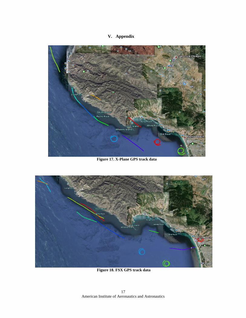
I. Flight Simulator GPS Data

The final set of data that was analyzed from the simulator tests was the GPS latitude and longitude coordinate

outputs. Figures 17 and 18 in the Appendix show the GPS tracks of all the tests performed in FSX and X-Plane

respectively. The output data from the simulators was then converted to a Google Earth compatible file which was

then uploaded to Google Earth for viewing. Overall the GPS data from both FSX and X-Plane was accurate and

could prove useful for further analysis of a multitude of simulation based tests.


16

IV. Conclusion

In summary, the project as a whole was successful in completing its main objectives of comparing the

capabilities of two different types of flight simulation engines and investigating the ins and outs of flight test in

general. Ultimately the data presented did not show with any certainty that FSX or X-Plane was any more accurate

than the other; however, the data did show that both simulators have extremely accurate models when compared to

the actual aircraft. Despite a few inconsistencies because of pilot error, the test data from both simulations was

remarkably similar to that of the actual aircraft. Furthermore, the data sets may have been more aligned had the tests

in all three cases been flown with more precision. Flight testing with high accuracy takes years of training and

meticulous mission planning, which ultimately is the cause for the high cost of the process. Through the use of

flight simulation, unlimited amounts of flight testing can be completed with unlimited possibilities and high

accuracy for a low cost.

The next step in validating the two simulations presented in this report would be to conduct higher precision

flight testing. Those tests could be done by using an autopilot to help take some of the workload off the test pilot.

Ultimately, the tests would become more accurate and more convincing conclusions could be made on the strengths

and weakness of each simulation. With regards to the output data presented in the results section, FSX and X-Plane

proved to have very similar results; however, the two simulators differed with regards to user interface and ease of

use. X-Plane has a much larger and complex user interface than FSX, which allows for a more customizable

experience. Additionally, X-Plane’s ability to test virtually any aircraft configuration without the use of stability

coefficients is an enormous selling point. However, the FSX model and overall flight qualities, if a robust set of

stability derivatives are available, are superior to those in X-Plane. In closing, both FSX and X-Plane have limitless

potential for flight testing in the commercial and educational arenas.


17

Figure 18. FSX GPS track data

Figure 17. X-Plane GPS track data

V. Appendix


18

References

1Evans, M. B., and Schilling, L.J., “The Role of Simulation in the Development and Flight Test of the HiMAT Vehicle,”

NASA TM-84912, 1984. 2Kimberlin, R.D., Flight Testing of Fixed-Wing Aircraft, AIAA, Virginia, 2003, Chaps 4,15,21. 3Lockheed Martin., “Prepar3D Product Information and Overview,” URL: http://www.prepar3d.com/products/prepar3d-

client/#productinfo [cited 7 May 2011]. 4Laminar Research., “X-Plane Instructions Manual,”[Appendix A: How X-Plane Works]. 5Microsoft., “Microsoft’s Flight Simulator X Flight Model Overview,” URL: http://msdn.microsoft.com/en-

us/library/cc526961.aspx [cited 7 May 2011]. 6Sorton, E. F., and Hammaker, S., “Simulated Flight Testing of an Autonomous Unmanned Aerial Vehicle Using

FlightGear,” AIAA 2005-7083.

Table 3. X-Plane data output sample

Table 2. FSX data output sample

http://www.prepar3d.com/products/prepar3d-client/#productinfo

http://www.prepar3d.com/products/prepar3d-client/#productinfo

http://msdn.microsoft.com/en-us/library/cc526961.aspx

http://msdn.microsoft.com/en-us/library/cc526961.aspx

Date post:	02-Jan-2022
Category:	Documents
Upload:	others
View:	3 times
Download:	0 times

Flight Testing in a Simulation Based Environment

Documents