Flood and Coastal Erosion Risk Management: … Economic Valuation of Environmental Effects –...

Flood and Coastal Erosion Risk Management:

Economic Valuation of Environmental Effects

HANDBOOK for the Environment Agency for England and Wales

Revised March 2010

eftec 73-75 Mortimer Street London W1W 7SQ tel: 44(0)2075805383 fax: 44(0)2075805385 [email protected] www.eftec.co.uk

mailto:[email protected]

http://www.eftec.co.uk/

FCERM: Economic Valuation of Environmental Effects - Handbook

eftec March 2010

Prepared for the Environment Agency for England and Wales by: Economics for the Environment Consultancy (eftec) 73 – 75 Mortimer Street, London, W1W 7SQ Tel: 020 7580 5383 Fax: 020 7580 5383 www.eftec.co.uk Authors (in alphabetical order): Economists: Roy Brouwer, IVM and eftec associate Ece Ozdemiroglu, eftec Allan Provins, eftec Chelsea Thomson, eftec Robert Tinch, EFL and eftec Kerry Turner, UEA and eftec associate Flood risk management experts: Steve Dangerfield, Cascade Consulting (at the time) Albert Nottage, Cascade Consulting (at the time). Acknowledgements: The study team would like to thank the EA project manager, Bill Watts and the members of the Steering Group and the wider circulation group for their comment and input.

eftec offsets its carbon emissions through a biodiversity-friendly voluntary offset purchased from the World Land Trust (http://www.carbonbalanced.org) and only prints on 100% recycled paper.

http://www.eftec.co.uk/

http://www.carbonbalanced.org/

FCERM: Economic Valuation of Environmental Effects – Summary

eftec March 2010

HANDBOOK SUMMARY


eftec i March 2010

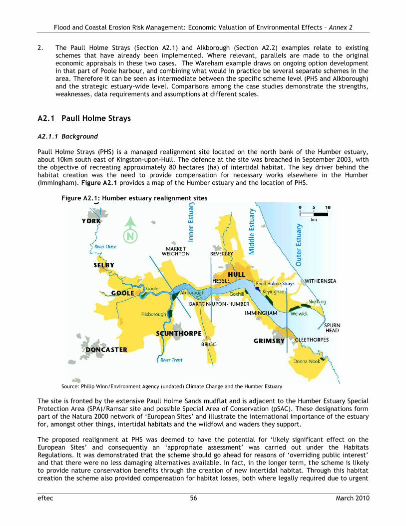
1. INTRODUCTION This work was commissioned by the Environment Agency for England and Wales (EA) to address the need to value environmental benefits from habitat creation and restoration within the context of flood and coastal erosion risk management (FCERM) projects and strategies. Official guidance – FCERM-Appraisal Guidance (AG) (EA, 2010) and the Green Book (HM Treasury, 2003) - allows for and encourages the valuation of the natural environment and the services provided by ecosystems. This work provides the necessary guidance.

Purpose

This guidance is intended for practitioners in the EA, Internal Drainage Boards, Local Authorities and contracted consultants responsible for the appraisal of FCERM schemes. It focuses specifically on the economic (monetary) value of environmental effects associated with FCERM schemes and is intended to augment the EA FCERM-AG and the Flood Hazard Research Centre (FHRC) „Multi-coloured Manual‟ and „Handbook‟ (Penning-Rowsell et al., 2005a; 2005b). Documentation produced under the title „Economic Valuation of Environmental Effects‟ includes this summary, a Handbook (Parts 1-3) for practitioners with associated annexes featuring case studies and a review of economic value evidence (Part 4) , and a more detailed Technical Report (Part 5) for the interested reader. Originally completed in August 2007, this material has been revised and updated in March 2010 to reflect recent developments in the valuation of the natural environment and ecosystem services. The guidance does not replace other analyses, such as Environmental Impact Assessment (EIA) and Strategic Environmental Assessment (SEA). In fact, the assessment of the economic value of environmental effects is built upon the information gathered by EIA and SEA.

Appraisal context

Economic appraisal and cost-benefit analysis (CBA) permit judgements as to the „value for money‟ of a given FCERM scheme and also the ranking of competing schemes1. This guidance applies to all schemes for which economic appraisal is required; from a site-specific level up to a wider and more strategic level, covering both inland water (flood risk management) and coastal (flood risk and coastal erosion risk management) contexts. Estimating the economic value of environmental effects is based on the following: I. Ecosystem services approach: this is a framework for assessing the goods and services provided by

ecosystems, where environmental effects relate to a loss or gain of one, a group, or all of the services of the ecosystems (see also Defra, 2007). The categorisation of ecosystem services used in this guidance is based on the Millennium Ecosystem Assessment (MEA, 2005) and features provisioning, regulating, supporting and cultural services.

II. Economic value: is a concept that underpins CBA and measures changes in wellbeing via the trade-off between money and changes in the quality or quantity of a resource, as revealed by the preferences of individuals (so-called willingness to pay or willingness to accept).

III. Economic valuation methods: provide techniques for estimating the economic value of changes in goods and services such as those associated with ecosystem services and potentially affected by FCERM schemes. These include market prices, revealed preference and stated preference methods, although, depending on the nature of the good in question, the extent to which these provide a full account of total economic value varies.

IV. Value transfer (also known as „benefits transfer‟): is the main component of this guidance. It allows existing economic value evidence to be used to estimate the monetary value of environmental effects associated with FCERM schemes. Although value transfer is used extensively and is a valuable input to

1 See FCERM-AG and FHRC documents for details of the overall CBA framework and decision criteria in the context of flood and coastal erosion risk management.


eftec ii March 2010

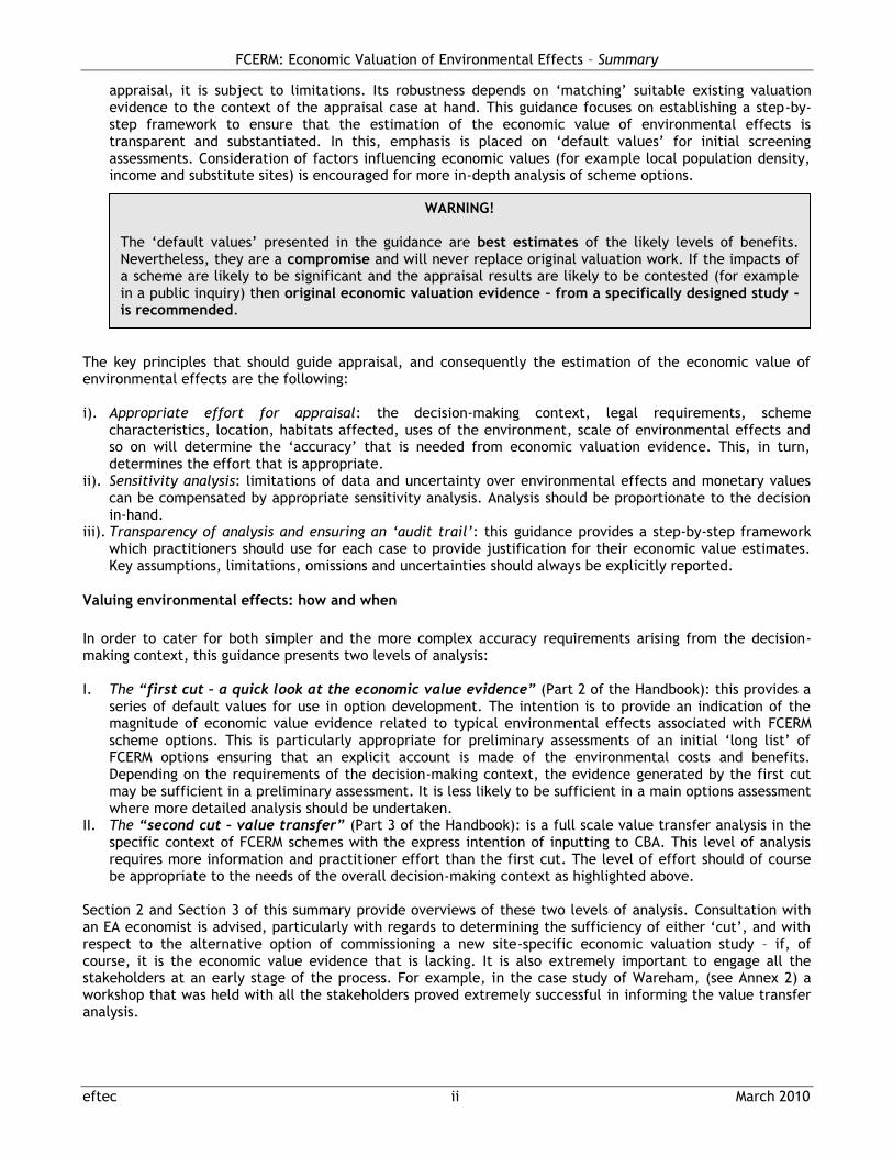
appraisal, it is subject to limitations. Its robustness depends on „matching‟ suitable existing valuation evidence to the context of the appraisal case at hand. This guidance focuses on establishing a step-by-step framework to ensure that the estimation of the economic value of environmental effects is transparent and substantiated. In this, emphasis is placed on „default values‟ for initial screening assessments. Consideration of factors influencing economic values (for example local population density, income and substitute sites) is encouraged for more in-depth analysis of scheme options.

The key principles that should guide appraisal, and consequently the estimation of the economic value of environmental effects are the following: i). Appropriate effort for appraisal: the decision-making context, legal requirements, scheme

characteristics, location, habitats affected, uses of the environment, scale of environmental effects and so on will determine the „accuracy‟ that is needed from economic valuation evidence. This, in turn, determines the effort that is appropriate.

ii). Sensitivity analysis: limitations of data and uncertainty over environmental effects and monetary values can be compensated by appropriate sensitivity analysis. Analysis should be proportionate to the decision in-hand.

iii). Transparency of analysis and ensuring an ‘audit trail’: this guidance provides a step-by-step framework which practitioners should use for each case to provide justification for their economic value estimates. Key assumptions, limitations, omissions and uncertainties should always be explicitly reported.

Valuing environmental effects: how and when

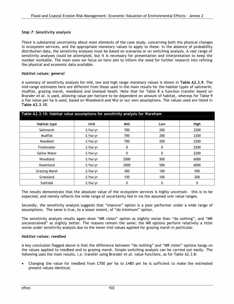
In order to cater for both simpler and the more complex accuracy requirements arising from the decision-making context, this guidance presents two levels of analysis:

I. The “first cut – a quick look at the economic value evidence” (Part 2 of the Handbook): this provides a

series of default values for use in option development. The intention is to provide an indication of the magnitude of economic value evidence related to typical environmental effects associated with FCERM scheme options. This is particularly appropriate for preliminary assessments of an initial „long list‟ of FCERM options ensuring that an explicit account is made of the environmental costs and benefits. Depending on the requirements of the decision-making context, the evidence generated by the first cut may be sufficient in a preliminary assessment. It is less likely to be sufficient in a main options assessment where more detailed analysis should be undertaken.

II. The “second cut – value transfer” (Part 3 of the Handbook): is a full scale value transfer analysis in the specific context of FCERM schemes with the express intention of inputting to CBA. This level of analysis requires more information and practitioner effort than the first cut. The level of effort should of course be appropriate to the needs of the overall decision-making context as highlighted above.

Section 2 and Section 3 of this summary provide overviews of these two levels of analysis. Consultation with an EA economist is advised, particularly with regards to determining the sufficiency of either „cut‟, and with respect to the alternative option of commissioning a new site-specific economic valuation study – if, of course, it is the economic value evidence that is lacking. It is also extremely important to engage all the stakeholders at an early stage of the process. For example, in the case study of Wareham, (see Annex 2) a workshop that was held with all the stakeholders proved extremely successful in informing the value transfer analysis.

WARNING! The „default values‟ presented in the guidance are best estimates of the likely levels of benefits. Nevertheless, they are a compromise and will never replace original valuation work. If the impacts of a scheme are likely to be significant and the appraisal results are likely to be contested (for example in a public inquiry) then original economic valuation evidence – from a specifically designed study - is recommended.


eftec iii March 2010

2. THE FIRST CUT – A QUICK LOOK AT THE ECONOMIC VALUE EVIDENCE The first cut establishes the likely importance of environmental benefits to the scheme or strategy in hand. It provides an indication of the magnitude of economic value evidence from the literature. This may be used to highlight the scale of the impact and to focus on the most important environmental effects.

Typically the first cut applies to the preliminary stages of an appraisal case, where all technically feasible options should be considered. The explicit consideration of the potential monetary value of environmental effects should ensure that FCERM schemes that provide environmental benefits are credited with those benefits and not dismissed as generators of cost alone. Retaining such schemes from an initial selection exercise may require that more information is collated on the potential environmental effects. This may entail more detailed analysis concerning the economic value of these effects, as per the second cut.

Identify environmental effects The environmental effects of a scheme arise due to the changes it creates in an ecosystem (e.g. habitats degraded / lost or expanded / created). The changes in the ecosystem in turn, lead to changes in the services they provide and hence their impact on human welfare. This task should be informed by EIA and SEA. Care should be taken to avoid double-counting between ecosystem processes and outcomes of those processes – for example nutrient cycling is a service that results in the outcome (among others), and hence benefit, of improved water quality.

[see Handbook: Section 2.1, Tables 2.1a and 2.1b]

Select appropriate economic value evidence At this level of analysis, economic value evidence pertaining to environmental effects provides an indication of possible orders of magnitude. Here it is sufficient to apply economic values that are defined for broad habitat types such as inland, intertidal and salt marsh. The selection of any value(s) should be justified and reported for the purposes of an audit trail. Given the preliminary nature of the analysis and likely uncertainty concerning scheme details and environmental effects, it is more appropriate to consider a low-high range for any estimated value, rather than a single point estimate, whether it be a mid-point estimate, or a „low‟ or „high‟ estimate.

[See Handbook: Section 2.1, Table 2.2]

Assess sufficiency of first cut Here it should be determined whether further work is required to substantiate estimates of the economic value of environmental effects. In most cases the first cut analysis will not be sufficient for direct use in CBA particularly if a scheme is progressed beyond an initial „long-list‟ of options. Overall the key criteria for determining whether to proceed beyond the first cut are:

Is the range of economic value estimates from the literature sufficiently large to warrant including the scheme into the list of possible options?

Is more precise economic value evidence necessary? and

To what extent does more accurate environmental benefit assessment (additional information) outweigh the cost of searching for more accurate information?

[See Handbook: Section 2.2, Table 2.3]


eftec iv March 2010

3. THE SECOND CUT – VALUE TRANSFER The second cut provides monetary estimates of environmental effects of FCERM schemes that may be used as an input to CBA. It also provides a framework for ordering non-monetary information on environmental effects for valuation and appraisal purposes. The methodology is sequential.

Step 1: FCERM options

Describe the FCERM option(s) to be appraised

CO

NT

EXT

FO

R V

ALU

ATIO

N

Step 2: Specify environmental baseline

Baseline conditions should be informed by EIA and SEA and presented in terms of relevant ecosystem services and the benefits derived from them, accounting for how these are likely to change during the appraisal time horizon. This permits the estimation of net environmental effects (costs or benefits); i.e. the difference between the baseline for the analysis and the FCERM scheme.

Step 3: Environmental effects

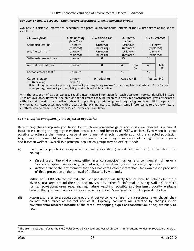
(a) Identify effects in terms of potential habitat creation or damage and the likely scale and timing of these.

(b) Provide qualitative assessment to link effects to changes in the provision of ecosystem services.

(c) Provide quantitative assessment of effects (e.g. hectares of habitat, tonnes of carbon).

Step 4: Define and quantify the affected population

Assess the type and scale of the affected population which may consist of users (local residents and visitors) and non-users (if likely to be a significant concern). For different environmental effects, the size of the relevant user/non-user population may differ (e.g. carbon is a global pollutant).

Step 5: Economic value of environmental effects

(a) Select relevant studies and valuation evidence. The Handbook details criteria for matching existing valuation evidence to the appraisal case. Annex 1 provides „look-up‟ tables for select inland and coastal habitat types.

(b) Transfer value estimates making adjustments where necessary and report these clearly. Annex 2 presents practical examples of unit and function transfers.

VA

LU

E T

RA

NSFER

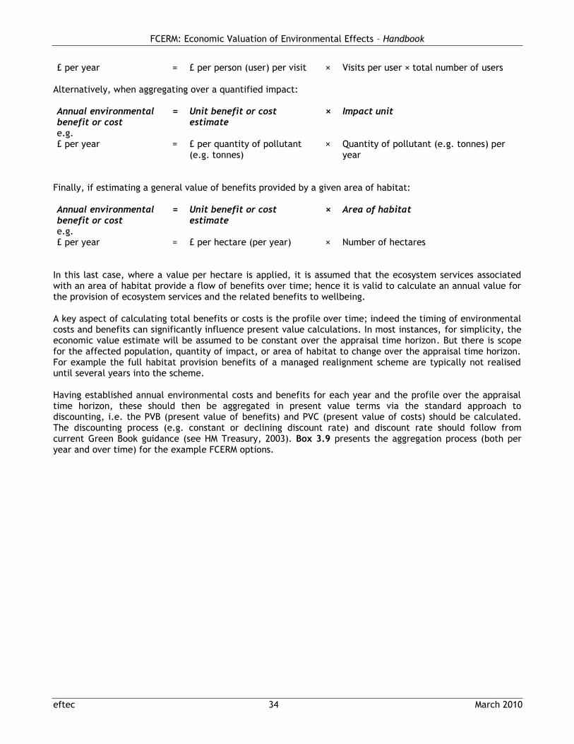
Step 6: Calculate monetary costs and benefits

Estimate annual environmental cost or benefit (e.g. £/yr × impact/yr) accounting for profile of costs and benefits over the appraisal time horizon. The present value of costs and benefits should then be calculated (see spreadsheet template).

Step 7: Sensitivity analysis

Assess the effect that different assumptions made in previous steps have on estimates of environmental costs and benefits, including: (i) estimates of environmental effects; (ii) estimates of affected population; (iii) unit economic values (e.g. „low‟, „medium‟, „high‟); and (iv) components of a function transfer. Where environmental costs and/or benefits are likely to be a determining factor, switching analysis and benefit thresholds should be considered.

SEN

SIT

IVIT

Y

Step 8: Combine monetary and non-monetary expressions of environmental effects

Provide detailed (even if only qualitative) assessment of the environmental effects that cannot be expressed in monetary terms. The ecosystem services framework allows for an explicit account to be made for monetised and non-monetised items.

R

EPO

RT

ING

Step 9: Reporting Make the assessment of economic value available to the wider decision-making process and provide an audit trail. Attention should be paid to: (i) uncertainty concerning estimates of environmental effects (e.g. timing, magnitude and significance); (ii) assumptions embodied in estimates of the relevant population; (iii) assumptions entailed in the transfer of economic values or functions; (iv) the potential significance of any incomplete information or non-monetised impacts, and (v) caveats associated with the resulting value estimates.


eftec v March 2010

In some instances it may not be necessary to go through all nine steps of the second cut. However it is not possible to be prescriptive about when all or part of the methodology would suffice since this depends entirely on the decision-making context in question. A number of key questions bound the scope of the process: i). Before: is value transfer appropriate for the needs of the decision-making context? ii). During: is a complete value transfer analysis possible? and iii). Before and during: is a new economic valuation study warranted (in preference to value transfer)? When unclear, consult an EA economist. Finally, it is important to stress that this document represents the start of a continuing process. In particular value evidence, but in time also the methodology, should be periodically updated to reflect the most recent developments.

FCERM: Economic Valuation of Environmental Effects – Handbook

eftec March 2010

ECONOMIC VALUATION OF ENVIRONMENTAL EFFECTS

HANDBOOK


eftec March 2010

TABLE OF CONTENTS

PART 1: INTRODUCTION 1.1 Who is this Handbook intended for? ................................................................................ 1 1.2 The policy need for the Handbook and links to other appraisal guidance and processes ................ 1 1.3 Could this Handbook assist you? .................................................................................... 2 1.4 Key concepts of the Handbook ...................................................................................... 4 1.5 Key principles for estimating the economic value of environmental effects ............................... 6 1.6 How and when to use this Handbook .............................................................................. 7 1.7 Updates to the Handbook ............................................................................................ 9

PART 2: THE FIRST CUT

2.1 A quick look at the available economic value evidence ....................................................... 10 2.2 Is the first cut sufficient? ........................................................................................... 15

PART 3: THE SECOND CUT

3.1 Value transfer in the context of FCERM schemes ............................................................... 17 3.2 What is the potential for value transfer for your scheme? .................................................... 18 3.3 Undertaking value transfer – Steps 1-9 ........................................................................... 22

STEP 1: FCERM OPTION(S) ................................................................................................ 22 STEP 2: SPECIFY ENVIRONMENTAL BASELINE CONDITIONS .......................................................... 22 STEP 3: ENVIRONMENTAL EFFECTS ...................................................................................... 23 3A. Identify environmental effects ................................................................................ 23 3B. Qualitative assessment of environmental effects ......................................................... 25 3C. Quantitative assessment of environmental effects ....................................................... 25 STEP 4: Define and quantify the affected population .............................................................. 27 STEP 5: ECONOMIC VALUE OF ENVIRONMENTAL EFFECTS ........................................................... 30 5A. Selecting relevant studies ...................................................................................... 30 5B. Transferring value estimates .................................................................................. 32 STEP 6: CALCULATE MONETARY COSTS AND BENEFITS .............................................................. 33 STEP 7: SENSITIVITY ANALYSIS ........................................................................................... 35 STEP 8: COMBINE MONETARY AND NON-MONETARY EXPRESSIONS OF ENVIRONMENTAL EFFECTS ........... 37 STEP 9: REPORTING ........................................................................................................ 38

REFERENCES ............................................................................................... 40

PART 4: ANNEXES PART 5: TECHNICAL REPORT [see separate document]

FCERM: Economic Valuation of Environmental Effects – Handbook Part 1

eftec March 2010

PART 1: INTRODUCTION


eftec 1 March 2010

Part 1 overview This Handbook contains the outputs of the project titled: Flood and Coastal Erosion Risk Management: Economic Valuation of Environmental Effects (Parts 1 to 3). It is accompanied by two further documents: Annexes (Part 4) and Technical Report (Part 5). A summary document is also available. This first part of the Handbook introduces its purpose, key concepts and contents:

Section 1.1: describes the intended user group;

Section 1.2: presents the policy need for the Handbook and places it in the context of other appraisal guidance for flood and coastal erosion risk management (FCERM);

Section 1.3: indicates whether the Handbook can assist the user with their particular FCERM scheme option(s) under consideration;

Section 1.4: summarises the key concepts underlying the overall project and in particular the Handbook.

Section 1.5: outlines key principles pertaining to estimating the economic value of environmental effects.

Section 1.6: summarises the content of the different parts of the Handbook and how and when it is best to use them.

Section 1.7: describes updates to the Handbook since the original version completed in August 2007. Practitioners are encouraged to familiarise themselves with the background to the Handbook by reviewing Part 1 and Sections 1.1 to 1.6. More experienced users should refer to Parts 2-5 as and when required.

1.1 Who is this Handbook intended for?

This Handbook is aimed at appraisal practitioners in the Environment Agency for England and Wales (EA) and other relevant operating authorities; Internal Drainage Boards with respect to water level management, and Local Authorities with flood defence and coastal erosion responsibilities. The guidance contained within the Handbook is largely non-technical, although inevitably familiarity with some concepts of economic analysis is useful. A more comprehensive review of such concepts and policy appraisal context for the Handbook is provided by the accompanying Technical Report (Part 5). Throughout the Handbook, reference to the relevant sections of the Technical Report (denoted as „TR‟) is made. Stages when the user would be advised to consult an Agency economist are indicated where relevant.

1.2 The policy need for the Handbook and links to other appraisal guidance and processes

The policy line in „Making Space for Water‟ (Defra, 2004; 2005) is generally expected to result in substantial environmental benefits as well as providing public safety benefits from reduced flood risks in the longer term. The balancing of environmental and flood risk management gains and losses requires consideration of the economic (monetary) value evidence. The use of money as the common unit account allows for direct comparison of costs and benefits of FCERM options. The Water Framework Directive (WFD) is also relevant in this context. WFD is an ecological directive and environmental benefits of floodplain restoration and other hydro-morphological changes contribute to good chemical and ecological status of water bodies, and are therefore considered important WFD measures in many EU Member States. Coherence and consistency across policies are another important criterion to justify the emphasis on the environmental costs and benefits of alternative flood control policy. The purpose of this Handbook is to assist flood risk and coastal erosion management (FCERM) decision-making in estimating the economic (monetary) value of environmental gains and losses associated with FCERM schemes. This, in turn, should ensure that FCERM schemes that have environmental benefits are credited with these benefits and that environmental enhancements are not dismissed as cost generators alone. Overall the Handbook is intended to inform economic appraisal and cost-benefit analysis (CBA) inputs to decision-making for schemes ranging from a site-specific level up to a wider and more strategic level,


eftec 2 March 2010

covering both inland water (flood risk management) and coastal (flood risk management and coastal defence) contexts. The approach set out in the Handbook augments current appraisal guidance from: the HM Treasury Green Book (HM Treasury, 2003), which provides overall appraisal guidance for Central Government departments and executive agencies; Defra with respect to valuing ecosystem services (Defra, 2007); the Environment Agency FCERM Appraisal Guidance (FCERM-AG) (EA, 2010); and the Flood Hazard Research Centre (FHRC) „Multi-coloured Manual‟ and „Handbook‟ (Penning-Rowsell et al., 2005a; 2005b). The FHRC documents cover the entire likely range of impacts that may arise from flooding or coastal erosion, including flood damage to residential and non-residential properties, costs of disruption, losses and benefits of erosion, recreational gains and losses, effects on agriculture and environmental costs and benefits. The specific focus of this Handbook on estimating the economic value of environmental costs and benefits (including recreational gains and losses) is intended to provide a practical framework for applying the principles set out in FCERM-AG and the FHRC documents, with the Technical Report providing more detail on the link between this Handbook and the Multi-Coloured Manual. The Handbook does not replace other analyses (e.g. Environmental Impact Assessment (EIA), Strategic Environmental Assessment (SEA), stakeholder consultation) used to date. In fact, assessment of economic value of environmental effects is built upon the information gathered by EIA and SEA, and can also be one of the inputs to stakeholder consultation. Therefore, the Handbook should be used in conjunction with guidance for these processes.

1.3 Could this Handbook assist you?

Before you consider economic value evidence and hence consult this Handbook, ensure that the FCERM options you are considering are technically feasible. Options that are not technically feasible should not be considered for further appraisal. The flowchart in Figure 1.1 shows that there are two questions to answer to in order to determine whether this Handbook could assist you in a given case:

First, if the FCERM scheme you are considering is of a type that is covered by this Handbook, as listed in Table 1.1, this Handbook can potentially assist you. As Table 1.1 shows, a wide variety of FCERM options (with focus on soft engineering options) are covered by the Handbook; so, it is only in exceptional cases that a scheme may be outside the scope of this Handbook.

Second, if your FCERM scheme is legally required then a full cost-benefit analysis of options may not be required but it is still likely that some measure of value for money is needed. If this is the case, this Handbook could potentially help you. If the scheme is not legally required then this Handbook may help you to assess the economic value of environmental effects of different options as part of an FCERM appraisal.

As Table 1.1 highlights, the focus of this Handbook is FCERM schemes that are likely to involve environmental enhancements (e.g. creation of new habitats). At the strategic level, flood and erosion risk management for the coastline and estuaries is part of the Shoreline Management Plan (SMP) process, whereas flood risk management for fluvial systems is part of the Catchment Flood Management Plan (CFMP) process. Both CFMP and SMP have associated „strategic management policies‟, which define the suite of potential „risk management options‟. Note should also be made of the Water Framework Directive and River Basin Management Plans, since these are intended to integrate flood risk and coastal erosion risk management whilst enhancing the natural and human environment.


eftec 3 March 2010

Figure 1.1: Could this Handbook assist you?

Table 1.1: FCERM Schemes covered by this Handbook

Inland Water (Flood Risk Management)

Coastal (Flood Risk Management and Coastal Defence)

Strategy Example Scheme(s) Strategy Example Scheme(s)

No active intervention Do nothing1

Hold the line Maintain/improve hard defences; Foreshore re-charge

Reduce existing flood risk management actions

Abandonment of defences1

Advance the line New hard defences

Manage flood risk at current level Maintain existing defences Management realignment

Abandon defences1; regulated tidal inundation

Sustain current level of flood risk into the future

Land use/management change; flood storage

No active intervention Do nothing1

Action to reduce flood risk Land use/management change; flood storage

Increase frequency of flooding Re-connect floodplain

Note: 1These schemes may not always be viable options; for example if existing (legal) safety levels are unlikely to be met if „do nothing‟ will not be selected. However, all options ought to be considered at least at the outset of an assessment for completeness.

NO or partially, but still need to make a business case

Is your scheme legally

required?

This Handbook can potentially assist you in assessing the value for

money of an FCERM scheme

This Handbook can potentially assist you

in appraising the

FCERM scheme

NO

Is your scheme covered in this

Handbook? See Table 1.1

YES

YES

This Handbook cannot assist you on this

occasion


eftec 4 March 2010

1.4 Key concepts of the Handbook

As noted above, this Handbook is intended to assist the appraisal practitioners in estimating the economic value of environmental costs and benefits associated with FCERM schemes. The main component is a process for using existing evidence from previously undertaken studies on the economic value in the relevant appraisal context. This is known as value transfer (and is also often referred to as „benefits transfer‟). The other key component featured in the Handbook is that of the ecosystem services approach (see also Defra, 2007). This is a conceptual framework for assessing the goods and services generated by ecosystems (or habitats), where environmental costs and benefits relate to a loss or gain of one, a group, or all of the services of the ecosystems affected by flooding, erosion and/or FCERM schemes. The following summarise four key concepts underlying the approach adopted in the rest of the Handbook. The discussion is a simplified summary of the conceptual discussion in the Technical Report. In order to put the Handbook into the correct conceptual context, this is essential reading when the Handbook is first used, unless the user is already familiar with these concepts. Further detail can be found in the Technical Report. Ecosystems services approach The ecosystem services approach is a term that has come to describe a basis for analysing how people are dependent upon the condition of the natural environment. The approach explicitly recognises that ecosystems and the biological diversity contained within them contribute to human wellbeing (or „welfare‟ in economic terminology). This contribution extends beyond the provision of goods such as food and fuel, to services which support life by regulating essential processes such as flood risk management. The categorisation of ecosystem services used in this Handbook is presented Figure 1.2. It is adopted from the UN Millennium Ecosystem Assessment (MEA) (MEA, 2005) and includes the four subsets of services: provisioning, regulating, supporting and cultural services2.

Figure 1.2: Ecosystem Services Categories

Provisioning services

Products obtained from

ecosystems

• Food

• Fresh water

• Fuel wood

• Fibre

• Biochemicals

• Genetic resources

Regulating services

Benefits obtained from

regulation of ecosystem

processes

• Climate regulation

• Disease regulation

• Water regulation

• Water purification

• Pollination

Cultural services

Nonmaterial benefits

obtained from

ecosystems

• Spiritual and religious

• Recreation and tourism

• Aesthetic

• Inspirational

• Educational

• Sense of place

• Cultural heritage

Supporting services

Services necessary for the production of all other ecosystem services

Soil formation Nutrient cycling Primary production

Source: Ecosystems and Wellbeing: a Framework for Assessment (MEA, 2003)

2 For further detail of ecosystem services see the Technical Report [TR 3.1]. Note that in Parts 2-4 of the Handbook, consideration of cultural services is limited to recreation and tourism, aesthetic, education and cultural heritage, which fit within the conceptual basis of economic value. Spiritual, religious, inspirational and sense of place aspects of ecosystems may be better interpreted as motivations for economic value.


eftec 5 March 2010

Categorisation of ecosystem services, however, is the starting point. Economic valuation is concerned with human wellbeing, and therefore it is necessary to establish how ecosystem processes result in benefits in these terms. From an economic valuation perspective, ecosystem services are the aspect of ecosystems that generate use and non-use values (see Section 1.4.2 below). For instance, „nutrients cycling‟ is a service which can result in the outcome of clean water. But while nutrients cycling and clean water provision are processes, only the latter is also a benefit (e.g. for household drinking water supply, abstraction for industry or agriculture and so on). Alternatively, the outcome „recreation‟ is not an ecosystem service. It is a benefit yielded from multiple inputs, i.e. natural, human, social and physical capital inputs. Hence in working with the ecosystem services approach, care is needed to distinguish between services in themselves and outcomes affecting wellbeing. Economic value Economic value, a concept which underpins CBA, is the sum of individuals‟ preferences for or against a change in the quality or quantity of environmental resources. For example, the economic value of an improvement in the quality or quantity of a given resource is defined as what individuals are willing to forgo in terms of some other resource in order to obtain the increase. The economic value of degradation in quality or quantity of a resource, on the other hand, is what individuals are willing to forgo to prevent this change. If the „other‟ resource is set as money, more specifically money income, it then becomes possible to express economic value in monetary terms, and compare, say, the environmental benefits of providing an improvement with the financial cost of such improvement. The trade-off between money and changes in the quality or quantity of the resource is termed as an individuals‟ willingness to pay (WTP) to secure a gain or avoid a loss; or an individuals‟ willingness to accept compensation (WTA) to forgo a gain or tolerate a loss. This reasoning holds for both resources that may be purchased in markets and resources that are non-market in nature (i.e. un-priced but still affecting individuals‟ wellbeing). The latter category is exemplified by environmental resources, such as those affected by FCERM schemes. The definition of economic value begs the question why individuals should have preferences about, and WTP or WTA for, environmental resources. The taxonomy of total economic value is useful to explain the motivations behind economic value. Details are in the Technical Report [TR 4.1]; here it suffices to note that the taxonomy consists of use value, which arises from either a direct or indirect interaction with a resource, and non-use value, which arises due to altruistic motives (for others‟ wellbeing), bequest motives (for the wellbeing of future generations) and/or for the sake of the resource itself (existence). Economic value (WTP or WTA) is determined by a number of factors that relate to the environmental resource (e.g. type of habitat); the change in the resource (e.g. expansion or reduction of the habitat area, or a change in the quality, as well as the scale of the change); the uses of the resource (e.g. recreation, fishing etc.); the factors determining non-use values (e.g. uniqueness of the resource), the number of people holding use and non-use values, and the socio-economic characteristics of the individuals affected (e.g. income, education, age, gender, opinions, etc.). Economic valuation methods A range of economic valuation methods3, have been developed to estimate the economic value of changes in the provision of non-market goods and services. The appropriateness of differing approaches is varied, with some providing estimates of economic value that are more accepted than others. For instance, using market prices to assess benefits from managed realignment in terms of the revenue from increased fish stocks may be relatively straightforward. But this will also provide an under-estimate of the economic value of this gain, since no account is made for any excess willingness to pay over market price, for the fish themselves, for non-use value reasons or other recreational benefits such as angling. Other approaches, such as those offered by revealed preference (using data from actual markets such as travel and housing influenced by environmental quality) and stated preference (use of questionnaires) methods attempt to estimate the full extent of willingness to pay, the latter group also being able to account for non-use value.

3 Valuation methods are also discussed in FHRC documents, although terminology may differ. The Technical Report [TR 4.2] provides summary of methods in relation to the components of Total Economic Value that may be estimated.


eftec 6 March 2010

Value transfer Value transfer is defined as the transposition of economic values estimated at one site (the „study‟ site) to another site (the „policy‟ site)4. The study site refers to the site where the original study took place, while the policy site is a new site where information is needed about the economic value of similar benefits. In the context of this Handbook, the policy site is the locality that is subject to FCERM appraisal. Value transfer is typically a quicker and lower cost approach to generating economic valuation evidence, compared to commissioning a specifically designed valuation study. This advantage of value transfer makes it a practical tool for policy appraisal given the time and resources constraints decision-making regularly faces. In particular, using value transfer can enable the effort of appraisal to remain proportionate to the proposal as required by the Green Book. However, „quick‟ and „lower cost‟ do not mean that value transfer is easy, and judgements are required as to when value transfer can be used and the level of effort that is appropriate in a given appraisal case. Overall, the more accurate the results need to be, the more effort is required. Further guidance on value transfer – which is consistent with the approach set out in this Handbook – is available from Defra (see eftec, 2010). In practice, there are several approaches to value transfer, which differ in the degree of complexity, the data requirements and the reliability of the results. The Technical Report [TR 4.3] sets out the main variants, namely:

(i) Unit value transfer (ii) Function transfer

value estimate [e.g. £/ha]

FCERM appraisal [£/ha] valuation function [e.g. £/ha = f (XSS)]

FCERM appraisal [£/ha = f (XPS)]

Where X is a set of factors that are found to statistically influence economic value, PS is the policy site and SS is the study site. Examples presented in this Handbook and the case studies in Annex 2 demonstrate both approaches (see Annex 1 and Annex 2 for further details). Although value transfer is used extensively in practice and is certainly a valuable input to appraisal, its limitations should be recognised. The robustness of value transfer depends on the success of the „matching‟ of policy site circumstances to an appropriate study site and the quality of the original economic valuation study. The factors checked for matching are those that are listed as determinants of economic value at the end of Section 2.1.1. Amongst these, some are usually not possible to match or even adjust for without collecting new information (e.g. attitudes of the local population), while others such as the site characteristics, changes in the resource and general socio-economic characteristics such as income are relatively easier to at least adjust for. Where there are significant differences between the study and policy sites, a number of strategies may be employed that „adjust‟ economic value estimates accordingly. These are detailed in Part 3.

1.5 Key principles for estimating the economic value of environmental effects

The combination of key concepts set out above and the overall FCERM context underlines a number of key principles that should guide the estimation of the economic value of environmental effects as set out in this Handbook: iv). Appropriate effort for appraisal: the decision-making context, legal requirements, scheme

characteristics, location, habitats affected, uses of the environment, scale of environmental effects and so on will determine the „accuracy‟ that is needed from economic valuation evidence. This, in turn, determines the effort that is appropriate. Practitioners need to determine the effort that assessment of

4 Value transfer is also often referred to as „benefits transfer‟, as was the case in the August 2007 version of this Handbook. This revised

version (March 2010) uses the term „value transfer‟ for the purposes of consistency with Defra guidelines for value transfer (see eftec, 2010). It is used since it recognises that the approach applies equally to market and non-market costs and benefits.


eftec 7 March 2010

economic value warrants in relation to the requirements of the overall decision-making process on a case-by-case basis.

v). Sensitivity analysis: limitations of data and uncertainty over environmental effects and monetary values can be compensated by appropriate sensitivity analysis. Analysis should be proportionate to the decision in-hand.

vi). Transparency of analysis and ensuring an ‘audit trail’: this guidance provides a step-by-step framework which practitioners should use for each case to provide justification for their economic value estimates. Key assumptions, limitations, omissions and uncertainties should always be explicitly reported.

1.6 How and when to use this Handbook

Parts 1 - 3 Starting with the FCERM scheme option(s), the user should think about the habitat and its goods and services affected by the option(s) which are then linked to the economic value. The information on the economic value of environmental effects is an input to the overall comparison of costs and benefits of a FCERM scheme option. The ultimate decision criterion for approval in a CBA is that all the benefits of a scheme outweigh all of its costs. If this is the case, the option should be included in the proposals assessed by the National Review Group (NRG) / Project Appraisal Board (PAB). If the opposite holds and costs outweigh benefits, then the scheme option should be dropped. If there is uncertainty, expert advice should be sought to help with the assessment. This comparison could take the form of expert assessment (e.g. when the initial list of likely options is discussed), stakeholder consultation (e.g. when the scheme is discussed with those affected locally or elsewhere)5 and a more formal analysis such as CBA. Economic value evidence could be an input to all three forms comparison. But depending on the inherent information requirements of the comparison, the legal requirements, the characteristics of the scheme, location, habitats affected, uses of the environment and so on, the detail and accuracy required of economic value evidence can differ. In order to cater for both the simpler and the more complex ends of the scale of requirements, this Handbook presents two levels of analysis: i). The “first cut – a quick look at the economic value evidence” (Part 2 of the Handbook)

The purpose of the “first cut” is to give the user an idea of the magnitude of economic value related to typical environmental effects associated with FCERM scheme options. The first cut is a summary of economic value evidence from the currently available literature and guidance on how to use these to inform analysis at this level of detail. A hypothetical example is presented in Part 2 to illustrate the approach.

The first cut is particularly useful at the initial stage of producing a long list of FCERM options and as part of a preliminary assessment of environmental costs and benefits. However, we would advise against using this level of analysis on its own to discard any options. The value evidence from the literature summarised here should assist the user in presenting the range of environmental costs and benefits so they can be taken into account in the decision-making process.

Depending on the requirements of the decision-making context, the evidence generated by the first cut may be sufficient in a preliminary assessment of options. Part 2 also presents a set of criteria to help the user to decide if the first cut would be sufficient. These criteria are inevitably incomplete, as it is not possible to pre-empt the information requirements of each and every FCERM decision-making context that may come about. Consultation with stakeholders and other Agency staff (including the economists) is always advisable. In general main options analysis should involve a complete value transfer exercise; i.e. a “second cut”.

5 Note that expert assessment and stakeholder engagement are also inputs to the more formal economic analysis like CBA and hence they

can also be inputs especially to value transfer as shown in Part 3 of the Handbook.


eftec 8 March 2010

ii). The “second cut – value transfer” (Part 3 of the Handbook):

A “second cut” should be pursued when evidence from the first cut is not sufficient for the purposes of decision-making. The second cut is essentially a step-by-step guide to value transfer in the particular context of FCERM schemes. A hypothetical example is again presented to illustrate the steps involved.

The second cut is more detailed than the first, and also requires more information and effort by the user, but, at the same time, it has a wider applicability. For example, while the findings of the first cut are not sufficient for CBA, the second cut should be in most cases. However, even in the second cut the use of value transfer should still be considered as a part of the exploratory process of finding preferred options, particularly given the potential errors involved in transferring economic values across sites, habitats, groups of people and through time (assuming stable preferences). Accordingly Part 3 also provides the decision-making criteria to help the user to decide whether the second cut approach is sufficient for their purposes. Where it is not, the alternative is to commission a new site-specific economic valuation study – that is, of course, if it is the economic value evidence that is lacking. This Handbook does not contain detailed information on commissioning a new economic valuation study since there is a large and involved literature on this. However, the possibility of commissioning an original study should not be discarded instantly and consultation with an EA economist is strongly advised.

Overall, what will determine the shift from the first to second cut and even to commissioning an original economic valuation study is the answer to the following question: what is an acceptable error in economic value estimates for the specific decision in the specific phase of the policy cycle at hand? While the Handbook and other parts of this report contain information that is intended to assist, this is a context-specific question only the user can answer for a given scheme. In addition, EA economists should also be consulted whenever possible. Part 4 In addition to Parts 1 – 3 (this document), the Handbook also comprises of an accompanying document containing supporting Annexes (Part 4). These include:

Annex 1: „Default‟ values for the first cut and an economic value „look-up‟ table for the second cut, along with on valuing greenhouse gas (GHG) emissions and carbon sequestration associated with FCERM schemes;

Annex 2: Case studies – three practical worked examples consisting of Paull Holme Strays (Humber estuary), Alkborough Flats (Humber estuary), and Wareham (Poole Harbour); and

Annex 3: Summary of economic value evidence that is used in Annexes 1 and 2. Spreadsheets that accompany the Annex 2 case studies are also available. Part 5 The Technical Report (Part 5) is a stand alone document which provides technical information on economic valuation, value transfer and ecosystems services to show the basis of the approach recommended in the Handbook, for the benefit of the interested user. While it is not necessary reading for the first cut, perusal of it over time will help familiarise the user with economic valuation of environmental effects. Note that the Technical Report has not been updated with the revisions to the Handbook in 2010. Practical use This Handbook presents a large amount of material that should be referred to as and when required. On the first time of use of the Handbook, we encourage users to read the entirety of both Parts 2 and 3 and at least one of the case studies. In subsequent uses, the first cut should not take more than a few minutes to find the relevant illustrative economic value evidence. Advice from EA economists, at least initially, should be sought for even the first cut, until the user is comfortable with the approach. More frequent and involved contact with EA economists for the second cut is advised. As mentioned above, the decision to commission a new valuation study should not be taken without consulting EA economists.


eftec 9 March 2010

1.7 Updates to the Handbook

This is the revised version of the Handbook. The main revisions in this version (March 2010) from the original version (August 2007) are:

Updated indicative values and ranges („default values‟) for the first cut (see Part 2). This reflects economic valuation evidence that has become available since 2007.

Addition of a „look-up‟ table of unit values (£/ha/yr) for the second cut, primarily based on the area of habitat and availability of substitute sites (see Part 3). This reflects economic valuation evidence that has become available since 2007.

The addition of Annex 1 to provide further detail on the specification of the first cut „default values‟ and the second cut „look-up‟ table.

Updated references to guidance relevant to appraisal of FCERM schemes and valuing environmental effects including: (i) FCERM-Appraisal Guidance (EA, 2010); (ii) revised guidance for carbon valuation (DECC, 2010); (iii) guidance for valuing ecosystem services (Defra, 2007); and (iv) practical guidelines for value transfer (eftec, 2010).

Updates to case studies6 (Annex 2) to reflect economic valuation evidence that has become available, since 2007 including revised guidance for carbon valuation.

Other minor edits have been made as necessary.

6 Note that as a result of the addition of the second cut look-up table, one case which featured in the 2007 version of the Handbook

(Essex Estuaries) has been omitted from this version. This example demonstrated a function transfer approach to value transfer which use of the look-up table now partially accounts for. In addition the Wareham case study has not been updated with the March 2010 revisions to the Handbook. This is primarily to retain consistency with versions of the case study that have been published elsewhere, for example in Defra (2007).


eftec March 2010

PART 2: THE FIRST CUT

A QUICK LOOK AT THE ECONOMIC VALUE EVIDENCE


eftec 10 March 2010

Part 2 overview This part of the Handbook consists of two sections:

Section 2.1 details the basis of the first cut, from establishing environmental effects to selecting economic value evidence, based on a set of „default values‟ derived from available evidence.

Section 2.2 sets out a discussion that to help decide whether the first cut is sufficient for the stage of decision-making you are contributing to.

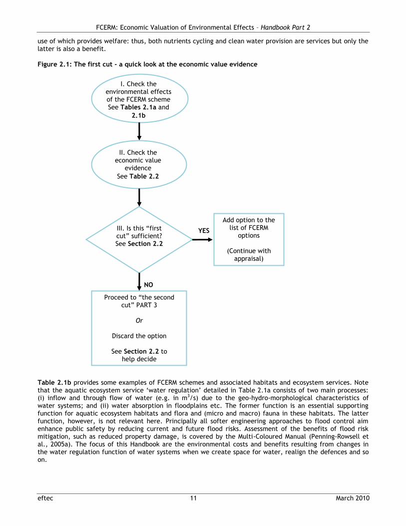
2.1 A quick look at the available economic value evidence

The basis of the approach to the first cut, which is intended as a quick look at the economic value evidence available in the literature, is presented in Figure 2.1. Its main purpose is to provide an input to the initial consideration of the list of potential FCERM scheme options. It provides an indication of the economic value evidence from the literature, which may be used to highlight possible orders of magnitude as to environmental benefits/costs and to focus on the most important environmental effects in terms of their economic value. The first cut involves three main tasks: I. Establishing the environmental effects of the FCERM scheme; II. Selecting economic valuation evidence; and III. Determining if the first cut assessment is sufficient. Details of the three tasks are set out below. I. Establish environmental effects of FCERM scheme The first step is to establish the type of environmental effects the FCERM scheme option you are considering is likely to have (note that the FCERM schemes considered should be technically feasible). This task should be informed by EIA and/or SEA outputs. An illustrative example is presented in Box 2.1. The environmental effects of a scheme arise due to the changes it creates in an ecosystem (e.g. habitats degraded / lost or expanded / created). The changes in the ecosystem in turn, lead to changes in the services they provide and hence their impact on human welfare. Table 2.1a shows the ecosystem services associated with the three main habitats that can be affected by FCERM schemes, which are freshwater and intertidal wetlands, and terrestrial habitats. The typology of ecosystem services is taken from the Millennium Ecosystem Assessment (MEA, 2005) and should be treated with care to avoid double-counting between ecosystem processes and outcomes of those processes. In this respect, differentiating between ecosystem services and the human welfare they provide is the key. For example, the outcome „recreation‟ is not a separate ecosystem service but a benefit provided by multiple services. Similarly, „nutrients cycling‟ is a service which can result in the outcome of clean water the

Box 2.1: Example - The FCERM options The stylised illustrative example here focuses on a specific site within an estuary. The overall estuary strategy includes both hard and soft engineering. At the specific site, there are four options of relevance. The first one is the do nothing option. For the first cut, the example will use Option 4 (full retreat). All four options are analysed in detail in the second cut in Part 3 of the Handbook.

Option Details

1. Do nothing No capital or maintenance expenditure

2. Maintain the line Improve existing hard defences to address sea level rise

3. Partial retreat Realign 250m landward

4. Full retreat Realign 500m landward


eftec 11 March 2010

use of which provides welfare: thus, both nutrients cycling and clean water provision are services but only the latter is also a benefit. Figure 2.1: The first cut - a quick look at the economic value evidence

Table 2.1b provides some examples of FCERM schemes and associated habitats and ecosystem services. Note that the aquatic ecosystem service „water regulation‟ detailed in Table 2.1a consists of two main processes: (i) inflow and through flow of water (e.g. in m3/s) due to the geo-hydro-morphological characteristics of water systems; and (ii) water absorption in floodplains etc. The former function is an essential supporting function for aquatic ecosystem habitats and flora and (micro and macro) fauna in these habitats. The latter function, however, is not relevant here. Principally all softer engineering approaches to flood control aim enhance public safety by reducing current and future flood risks. Assessment of the benefits of flood risk mitigation, such as reduced property damage, is covered by the Multi-Coloured Manual (Penning-Rowsell et al., 2005a). The focus of this Handbook are the environmental costs and benefits resulting from changes in the water regulation function of water systems when we create space for water, realign the defences and so on.

I. Check the environmental effects of the FCERM scheme See Tables 2.1a and

2.1b

II. Check the economic value

evidence

See Table 2.2

III. Is this “first cut” sufficient? See Section 2.2

YES

NO

Proceed to “the second cut” PART 3

Or

Discard the option

See Section 2.2 to help decide

Add option to the list of FCERM

options

(Continue with appraisal)


eftec 12 March 2010

Table 2.1a: Ecosystem services for freshwater wetlands, intertidal habitats and terrestrial habitats Ecosystem services Freshwater wetlands

(inland marsh) Intertidal habitats

(saltmarsh & mudflat) Terrestrial habitats

Supporting services

Soil formation - - ●

Primary production ● ● ●

Nutrient cycling ● ● ●

Provisioning services

Ecosystem goods primary production fibre and construction products food and drink products medicinal and cosmetic products ornamental products renewable energy sources regenerative services

○ ○ ○ ○ ○ ○ ○

○ ● ○ ○ ● ○ -

● ○ ○ ○ ○ ○ ●

Fresh water Maintenance of surface water stores Groundwater replenishment

● ○

- -

- -

Biochemicals and genetics ○ ○ ○

Regulating services

Air quality regulation - - ○

Climate regulation Global climate (carbon sequestration) Local climate

● ○

○ ○

○ ○

Water regulation (flood risk mitigation) ● ● ○

Water quality (purification) Filtration of water Detoxification of water and sediment

● ●

○ ●

○ -

Pest regulation - - -

Disease regulation - - -

Pollination - - ●

Erosion regulation ● ● ●

Cultural services

Recreation and tourism ○ ○ ○

Aesthetic ○ ○ ○

Education ○ ○ ○

Cultural heritage ○ ○ ○

Note: Table shows services that may be provided (○); services of possible (relative) importance (●) and (-) where the ecosystem service is not relevant either to the specific ecosystem in general or in the conditions of the UK. Source: Based on eftec and Just Ecology (2006).

Table 2.1b: FCERM Schemes and associated habitats and examples of ecosystem services Example schemes Habitat creation /

enhancement Example environmental effects (based on ecosystem services approach)

Saline realignment Intertidal wetlands (mudflats), saltmashes

Water purification (capture of nutrients, heavy metals, TBT (Tributyl tin) and complex organic pollutants) Climate regulation (carbon sequestration) Siltation Ecosystem goods (fisheries enhancement) Recreation and amenity

Saline abandonment

Saline in-scheme habitat enhancement

Fluvial realignment Freshwater wetland (inland marsh), terrestrial habitats

Water purification (capture of nutrients, heavy metals, TBTs and complex organic pollutants) Siltation Ecosystem goods (fisheries enhancement) Recreation and amenity

Fluvial restoration

Fluvial infrastructure abandonment

Fluvial infrastructure reuse

Fluvial in-scheme habitat enhancement


eftec 13 March 2010

Using EIA and/or SEA outputs and reading through Tables 2.1a and b, you should be able to determine which habitat(s) the FCERM option(s) you are considering will affect or create and the type of ecosystem services that are typically associated with those habitat(s). Note that the information in these two tables is based on the generalisations about types of schemes. If information about the scheme options is available from option scoping reports or preliminary environmental impact assessment, this should of course be used to inform the analysis. However, in general more detailed assessment is left to the second cut (value transfer). II. Select economic value evidence Once the type of habitat/environmental effects (ecosystem services) associated with your FCERM option(s) has been established, the next step is to select the relevant economic value evidence to provide an indication of the potential magnitude of environmental benefits/costs. Table 2.2 presents a set of „default values‟ based on available studies, for the purpose of the first cut only. Annex 1 provides further detail on the basis for the values and ranges reported, including habitat classifications.

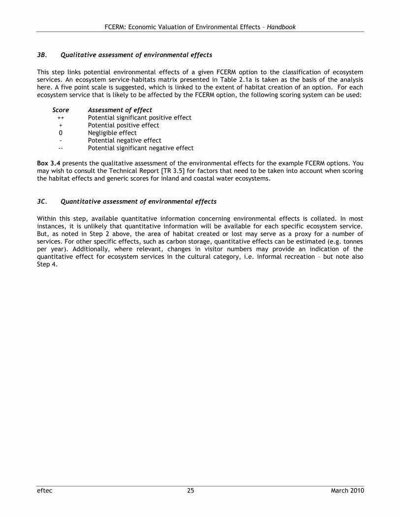
Table 2.2: Range of indicative economic values („default values‟) for different habitats (£/ha/yr, 2008 prices)*

Habitat & ecosystem service provision1

Indicative value Range Units

Inland marsh: water quality

improvement, recreation (non-consumptive), biodiversity,

aesthetic amenity

~1300 200 - 4300 /ha/yr

Saltmarsh: water quality


aesthetic amenity

~1400 200 - 4500 /ha/yr

Intertidal mudflat: water quality improvement, recreation (non-

consumptive), biodiversity, aesthetic amenity

~1300 200 – 4300 /ha/yr

Peat bog: water quality


aesthetic amenity

~300 0 - 1000 /ha/yr

Notes: * Reported values and ranges should be interpreted as „indicative‟ based upon currently available evidence – Annex 1 and Annex 3 provide details on the source studies for these values. As new economic value evidence relevant to the above environmental effects becomes available, this table may need to be updated. It is advisable to consult an EA economist for the continued relevance of these estimates. 1 The value of carbon storage is not included in indicative values and ranges. See also Annex 1. The indicative economic value evidence reported in Table 2.2 is presented in terms of habitat type and associated ecosystem service provision (linking to Tables 2.1a and b). Users are encouraged to consider the reported range of values in their analysis rather than point estimates alone. The broad ranges of values reported - over a 300% increase on the upper end of the range from the indicative values – reflect the influence that various factors have on unit economic values. This includes aspects such as the size of habitat creation/enhancement site, the availability of substitute sites in the area, the size of the local and regional population and the types of ecosystem service provided by the site (see Annex 1). These are factors that should be accounted for in the second cut (Part 3) to provide a refined estimate of the economic value of environmental effects. In applying economic value evidence from Table 2.2 users should consider the following points:


eftec 14 March 2010

Ecosystem service provision: the indicative values presented in Table 2.2 are reported as including water quality improvement, recreation (non-consumptive, i.e. walking, nature watching, etc.), biodiversity (based on various supporting and provisioning services) and aesthetic amenity. These are the ecosystem services that are typically associated with FCERM habitat creation/enhancement schemes but may not be appropriate in all instances. Users should assess if this is the case. More sophisticated analysis in the second-cut can address the specific details of ecosystem service provision.

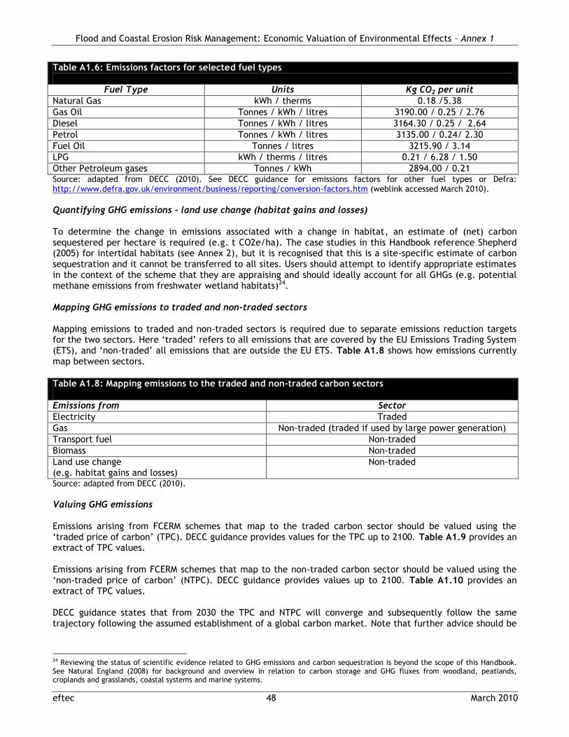
Carbon storage: the indicative values do not account for potential GHG emissions and sequestration of and carbon from habitats. If this is not addressed in the first cut it should be included in the second cut. Guidance for valuing carbon is provided by DECC (2010) – see also Annex 1 and Part 3.

Flood-risk mitigation: the indicative values do not account for potential flood risk mitigation benefits of habitat creation schemes (e.g. through provision of flood storage areas). This is to avoid double-counting with the estimation of benefits from protecting people and property (via the FHRC „Multi-coloured Manual‟).

Terrestrial habitats: While some evidence relating to terrestrial habitats does exist, it is not reported in Table 2.2 or Annex 3. It is recommended that an EA economist be consulted for schemes significantly impacting upon terrestrial habitats (e.g. in relation to potential overlap with FHRC Handbook and Manual guidance for agricultural land).

„Linear‟ schemes: the reported valuation evidence focuses on areas of habitat creation or loss, with no account for environmental effects that may be viewed as „linear‟; e.g. improvements to river bank habitats. This is informed by the assumption that „minor enhancements‟ to schemes should typically be viewed as best practice, rather than requiring cost-benefit justifications. Schemes for which the Handbook is potentially of use, such as flood-plain (re-)establishment, and setting back flood banks, are in general suitable for an „area-based‟ assessment (e.g. hectares of habitat created).

The environmental effects relevant for the example FCERM options described in Box 2.1 are presented in Box 2.2.

Box 2.2: Example – Assessing economic valuation evidence Both the do nothing and full retreat options are shown here:

Option Habitat created / environmental effects (ecosystem services)1

Relevant economic valuation evidence from Table 2.2

Comment / assumptions

1. Do nothing2 Some area of intertidal habitat exists and will be created

Existing evidence suggests that benefits from habitat creation could be significant. A „conservative‟ range of indicative values for habitat gain/loss: Mudflat: ~£200 - £4,300/ha/yr Saltmarsh: ~ £200 - £4,500/ha/yr No evidence available for saline lagoons but this could be in same range as mudflat and saltmarsh (£200 - £4,500/ha/yr)

Selection of value range reflects the expectation that recreational access to the site will be limited, i.e. suggesting a lower unit value all else equal. However at his stage uncertainty concerning habitat creation and availability of this habitat elsewhere, implies that a higher unit value may be considered.

4. Full retreat Areas of coastal habitat created (mudflat, saltmarsh, saline lagoons) with some loss of fronting mudflat and saltmarsh – larger area than „do nothing‟ and more certainty about the success of habitat creation

Notes: 1 This assessment should be based on existing information about the scheme and supporting information in Tables 2.1a and b. 2 In the second-cut, the approach is very much about the net change in the habitat and ecosystem services due to the FCERM option(s) (net of what would have happened in the baseline). However, here, there may not be sufficient time / information to assess the net effect. Therefore, the economic evidence from Table 2.2 concentrates on the types of habitats that the full retreat is likely to create. This difference may be more stark if different types of habitats are created by the baseline (do nothing) option and the „soft engineering‟ FCERM option.


eftec 15 March 2010

2.2 Is the first cut sufficient?

The main purpose of the first cut is to provide an input to the initial consideration of the list of potential FCERM scheme options as easily and quickly as possible. It provides an indication of the magnitude of economic value evidence from the literature regarding the environmental impacts involved on the basis of habitat types used as proxy. But the first cut is just that – it‟s a quick look at the economic value evidence available in the literature. It is not a value transfer exercise. III. Determining if the first cut assessment is sufficient Estimates of environmental benefits and costs of FCERM schemes based on a first cut assessment will not, in most if not all cases, be sufficient for direct use in a CBA without further work to substantiate the relevance of the estimates to the FCERM scheme option(s) and location(s) under consideration. For this further work on environmental effects of the FCERM option and how to take note of other local factors is required and is detailed the second cut (Part 3 of the Handbook). The potential inappropriateness of the default values presented in Table 2.2 could fall anywhere between the following two extreme cases:

Even the lower bound estimate of a value for a given habitat type may be an over-estimate for your FCERM option, if, say, there are large areas of that habitat in the location of the option; the environmental change valued is smaller in the scheme location than in the studies from the literature and so on. If this is the case, it is necessary to proceed to the second cut (value transfer) in Part 3 for a fuller assessment of the economic value of environmental effects.

Even the upper bound estimate of a value for a given habitat type may be an under-estimate for the option you are considering, if, say, the habitat to be created by the scheme is the only one of its kind in the area, the change is much larger than the one studied in the literature, or the local population demand the habitat more than those involved in the study selected. If this is the case, it is necessary to proceed to the second cut (value transfer) in Part 3 for a fuller assessment of the economic value of environmental effects.

In addition to the above, Table 2.3 presents the overall decision-making criteria for deciding if the first cut is sufficient. When in doubt, it is advisable to consult an EA economist. Note that the second cut stops at value transfer, but after (or instead of) this you may wish to carry out an original valuation study. While this notional „third-cut‟ is not discussed in this Handbook, the user should keep the overall scope of economic valuation exercise from the first cut to a full scale original valuation study in mind when deciding the sufficiency of each cut.


eftec 16 March 2010

Table 2.3: Overall decision-making criteria for deciding if the first cut approach is sufficient Criterion Implications

1. Is the range of economic value estimates from the literature sufficiently large to warrant including the scheme into the list of possible options? Note: “sufficiently large”?: The range of benefits estimates is larger than incremental costs of enhancements.

Yes – add to the list of FCERM scheme options to go to NRG. No – do not rush to conclude that the option should be discarded without exploring the economic value evidence further. For this, see criterion (2).

2. Is more precise economic value evidence necessary?

Yes – if the expected environmental benefits are such that they can play a decisive role in the CBA underpinning the FCERM option(s). If so, the user needs to identify which types of environmental impacts can be expected from different degrees of retreat or other alternative (non-traditional „hold the line‟ policy) flood and erosion control schemes. No – otherwise.

3. To what extent does more accurate environmental benefit assessment (additional information) outweigh the cost of searching for more accurate information?

Weight the accuracy, which further work in the second cut will bring, against the additional effort. You may wish to consider other pros and cons of all options considered and other factors that you think are important. For example, if the financial cost of the scheme is relatively low, further analysis of environmental benefits may not be necessary to support the scheme. However, if the cost of the scheme is relatively high, or even if the first cut shows high environmental benefits, evidence with greater accuracy may be required to support the scheme. What can be defined as „relatively high or low‟ depends on the specific circumstances of the decision being made. Factors that are beyond economic value assessment such as distributional effects (e.g. across different user groups, regional / local employment impacts) and so on should also be considered but are not within the scope of this Handbook.


eftec March 2010

PART 3: THE SECOND CUT

VALUE TRANSFER


eftec 17 March 2010

Part 3 overview This part of the Handbook consists of three sections:

Section 3.1 provides an overview of value transfer in the context of FCERM schemes;

Section 3.2 provides a discussion on the potential usefulness of value transfer (the second cut) for the appraisal of the FCERM scheme(s) you are considering. Decision criteria to assess whether the second cut is sufficient or a new economic valuation study is required are also presented here; and

Section 3.3 provides detailed guidance on the value transfer and an example illustrating this guidance.

3.1 Value transfer in the context of FCERM schemes

Value transfer in the context of FCERM schemes involves a methodology of nine main steps7:

While the overall aim of this second cut is to provide monetary estimates of environmental impacts that may enter into cost-benefit calculations, the above steps also provide a framework for ordering non-monetary information on environmental effects for valuation and appraisal purposes:

Steps 1 to 4 set the context for the economic valuation and the value transfer exercise. This is concerned with defining the effects in terms of changes to ecosystem services, and providing both qualitative (descriptive) and quantitative information on these effects.

7 Note that the methodological steps set out here are consistent with Defra guidelines (eftec, 2010) for the use of value transfer for valuing environmental impacts in policy and project appraisal.

Step 1 Define FCERM scheme option(s)

Context for Valuation

Step 2 Specify the environmental baseline

Step 3

Environmental effects: (a) Identify environmental effects (b) Qualitative scoring of environmental effects (c) Quantifying environmental effects

Step 4 Define and quantify the affected population(s)

Step 5

Economic value of environmental effects (a) Selecting relevant studies (b) Transferring value estimates

Value Transfer

Step 6 Calculate monetary costs or benefits

Step 7 Sensitivity analysis

Sensitivity

Step 8 Combine monetary and non-monetary expressions of environmental effects

Reporting Step 9 Reporting


eftec 18 March 2010

Steps 5 and 6 deal with monetary expressions of environmental costs and benefits and are concerned with identifying suitable economic value information that may be related to a given FCERM scheme option. Much emphasis should be placed on identifying potential limitations and uncertainty in the transfer process. That said, uncertainty will not only be associated with the economic valuation part of the assessment; the specification of environmental impacts will also be subject to uncertainty.

For this reason, sensitivity analysis plays a key role in the methodology, as set out in Step 7.

Finally Steps 8 and 9 detail recommendations for combining different types of information and reporting of the results.

The methodology is sequential: however, it may not be necessary to go through all nine steps in each appraisal case. In some cases, for example, qualitative or quantitative descriptions of environmental effects (Step 3) may suffice. If so, the analysis could stop. It is not possible to be prescriptive about when all or part of the methodology would suffice since this depends entirely on the dynamics of the decision-making context in each case (e.g. the popularity of FCERM scheme(s) amongst stakeholders, legal requirements, regulatory requirements and so on). This part of the Handbook presents all nine steps as though all were necessary. The user can stop at any step that they find sufficient for their purposes.

3.2 What is the potential for value transfer for your scheme?

A number of key questions bound the scope of the value transfer process:

Before: is value transfer appropriate for the needs of the decision-making context?

During: is a complete value transfer analysis possible?

Before and during: is a new economic valuation study warranted (in preference to value transfer)? Whether value transfer is an appropriate approach for a specific decision-making context can be established straight away (see Table 3.1 for a non-exhaustive list of criteria).

Table 3.1: Criteria for deciding if value transfer is appropriate

Criterion Implications

1. Is your analysis informing in a public inquiry or is a public inquiry in the near future likely?

Yes – value transfer would not be appropriate, more accurate evidence would be required. No – value transfer would be appropriate so proceed to Section 3.3

2. Is the Environment Agency making a case to Defra / HM Treasury?

Yes – value transfer may not be appropriate and more accurate evidence may be needed. No – value transfer would be appropriate so proceed to Section 3.3.

3. Is there an on-going dialogue with the Government about the consequences of the Water Framework Directive or other relevant Directives?

4. Is there an internal (within EA) appraisal about the re-allocation of funds across different functions?

The second question, the feasibility of value transfer, depends on the availability of information on the environmental impacts and economic values. Therefore, before the criteria presented in Table 3.2 can be judged for a specific FCERM scheme option and location, some of the initial steps of value transfer need to be implemented.


eftec 19 March 2010

Table 3.2: Criteria for deciding if value transfer is possible

Criterion Implications

1. Is there sufficient qualitative and quantitative environmental effect information (from Steps 1-3C) that can input to a value transfer exercise?

Yes – value transfer is possible. No – value transfer (or economic valuation) is not possible if environmental effect information is not available or sufficient.

2. Is there at least one valuation study that covers the same or similar human population? (Step 4)

Yes – value transfer possible. No – value transfer could still be possible (e.g. through adjustments to socio-economic characteristics); or a new valuation study may have to be commissioned (See Table 3.3); or non-economic evidence will have to be used.

3. Is there at least one valuation study that took place at the same or similar location? (Step 5A)

Yes – value transfer is possible. No – value transfer could still be possible (e.g. through adjustments); or a new valuation study may have to be commissioned (See Table 3.3); or non-economic evidence will have to be used.

4. Is there at least one valuation study that covers the same or similar habitat? (Step 5A)

Yes – value transfer is possible. Table 2.2, Annex 1 and Annex 3 present the economic value evidence in terms of the habitats they apply to. So long as your scheme affects one or more of the three main habitats (i.e. intertidal wetlands, freshwater wetlands and terrestrial habitats), this criterion would be met. No – value transfer is not possible since there are no adjustment factors to cater for the ecological differences of habitats. A new valuation study may have to be commissioned (See Table 3.3), or non-economic evidence will have to be used.

Table 3.2 presents the criteria for deciding if value transfer is possible for the FCERM option(s) you are considering. A negative answer to the first question is an absolute rejection of the possibility of value transfer (and even, at least an immediate, application of a new valuation study). Negative answers to the other questions may indicate the impossibility of value transfer or the need for some adjustments to the available evidence or even commissioning a new economic valuation study. If the answers to questions 2-4 are all negative, then the only option for generating economic value evidence would be a new economic valuation study; but even then this decision may not be warranted. However, note that even if as a result of assessing the criteria in Tables 3.1 and 3.2, you decide value transfer is the appropriate approach, whether it is sufficiently robust or not can only be judged at the end of the exercise. Even when literature contains evidence similar to your case, the estimates at the end may lead to unacceptably high transfer errors. Therefore, only at the conclusion of the value transfer exercise, will you be able to fully assess the reliability and acceptability of the value estimate. The main objective you should keep in mind is the answer to the question that is also asked in the first cut: what is an acceptable error in economic value estimates for the specific decision in the specific phase of the policy cycle at hand? This is a context-specific question only the user can answer for a given scheme. If you conclude that value transfer would not be the appropriate or sufficient, the two alternatives are either to base your arguments on the FCERM option(s) on evidence other than economic value, or to commission a new economic valuation study. Table 3.3 presents criteria to help you decide if the latter is worthwhile. Priority should be given to a commonly applicable scheme so that its findings could be used for further value transfer. It is crucial that an EA economist is consulted at this stage to advise on establishing the need for a new study, prioritising the requirements for new studies across the country and, finally, preparing the specification for research.


eftec 20 March 2010

Table 3.3: Criteria for deciding if a new economic valuation study is warranted

Methodological Criteria Implications

How does the potential cost of such a new study compare with the value of the extra confidence it provides?

Seek advice from an EA economist

Is the scheme highly politicised in the local area (e.g. locally opposed)?

Yes – original valuation is probably not advisable as the political circumstances could make it impossible to detect economic preferences free from strategic behaviour. It could be argued that primary research could take place somewhere else with same habitat and similar conditions for factors determining economic value. No – original valuation can be considered.

How sensitive is the overall decision likely to be to the assessment of environmental effects?

Very sensitive – in consultation with stakeholders (and if there is time) a new economic valuation study may be warranted. Not very sensitive - then it may not be worth spending extra funds on an original study (however, if the first cut was not sufficient, then it‟s likely that the schemes that have made it to this stage are likely to have environmental effects that are crucial in the overall decision-making). “very” / “not very” are judgement based terms and depends on the individual case of site / scheme / decision-making context.

Figure 3.1 summarises the process of set out Tables 3.1 – 3.3 for establishing if value transfer is appropriate and possible for a given FCERM scheme appraisal.


eftec 21 March 2010

Figure 3.1: Summarising Tables 3.1 – 3.3 - is value transfer appropriate or possible?

Is value transfer

appropriate? See Table 3.1

Is value transfer possible?

See Table 3.2

Proceed through STEPS 5B – 9

See Section 3.3

NO

YES

NO

Use evidence other than economic value

Original economic valuation study See Table 3.3

Complete the

appraisal

Proceed through Steps 1 – 5A

See Section 3.3

YES


eftec 22 March 2010

3.3 Undertaking value transfer – Steps 1-9

STEP 1: FCERM OPTION(S)

This is a straightforward step that explicitly states the relevant FCERM option(s). See Table 1.1 above for the list of schemes that are covered in this Handbook. Box 3.1 shows Step 1 for the illustrative example. Note that all options selected at this stage should be technically feasible.

STEP 2: SPECIFY ENVIRONMENTAL BASELINE CONDITIONS

Appraisal of an FCERM scheme option must focus on net costs and benefits, where „net‟ refers to the difference between: (i) what will happen with the scheme option; and (ii) what would have happened without it. The latter, „the without case‟, is also known as the baseline. Thus, this step is concerned with describing the prevailing environmental conditions in the situation without the FCERM option(s) under consideration. The baseline conditions should be informed by EIA, SEA and other environmental assessment outputs and presented in terms of relevant ecosystem services and the benefits derived from them. When available data and knowledge allow, the ecosystem services approach is an ideal tool for a systematic description of the environmental baseline conditions. The most typical baseline is „do nothing‟, implying, in this case, that no further investments are made to maintain the existing flood and coastal erosion risk defences, and no further investments are made in new defences. Note that there could be both costs and benefits associated with the „do nothing‟ case. In fact, if the baseline „do nothing‟ involves (uncontrolled) flooding of land then that may have benefits of habitat creation quite similar to a FCERM scheme option that creates a similar habitat (e.g. a managed realignment option). However the lack of control over timing and extent of effects in the baseline case may cause problems, often flagged up in appraisals (as a way of demonstrating „do nothing‟ to be a non-starter). Health and safety liability, uncontrolled release of contaminants in existing structures, lost ability to maximise benefits could be amongst these problems. Therefore, in some cases, the net benefit of an FCERM scheme option could be an absolute amount of benefit (e.g. creation of a new habitat that would not be created in the baseline case). In others, the net benefit of the option may simply be due to the reduced uncertainty (or increased control) over the realisation of the same benefits. Box 3.2 presents the assessment of baseline conditions in terms of ecosystem services in the context of the example FCERM schemes.

Box 3.1: Example: Step 1 – The FCERM options The illustrative example which follows each step of value transfer focuses on a specific site within an estuary. The overall estuary strategy includes both hard and soft engineering. At the specific site, there are four options of relevance:

Option Details

1. Do nothing No capital or maintenance expenditure

2. Maintain the line Improve existing hard defences to address sea level rise

3. Partial retreat Realign 250m landward

4. Full retreat Realign 500m landward


eftec 23 March 2010

STEP 3: ENVIRONMENTAL EFFECTS

In this step potential environmental effects arising from FCERM options are mapped to ecosystem services. In the main, this depends on the changes (creation, enhancement, degradation) on the habitats concerned:

Step 3A and Step 3B are concerned with providing a qualitative assessment, with regards to significance and magnitude, of environmental effects. This information will have an important bearing upon the subsequent economic valuation steps.

Step 3C is the quantitative assessment of potential effects. Note that this step of the Handbook methodology will need to be informed by available information on the environmental effects of different options, i.e. from scoping studies and EIA and/or SEA outputs. Input from environmental assessment experts may also be required.

3A. Identify environmental effects

The intention here is to: (i) Identify FCERM options with potential to create or damage habitats and amalgamate options where

possible. Individual options may be grouped where outcomes are likely to be identical in terms of extent and timing of effects. For example, variants of a „hold the line‟ strategy may result in similar environmental effects (e.g. maintaining the status quo), but variants of a managed realignment strategy may require separate treatment, since these can result in different sizes, and possibly types, of habitat created over different timescales; and

(ii) Identify, for each discrete FCERM option/group, a number of habitat effect scales which link to: (i)

„quality‟ (in terms of desirability or non-desirability) of habitat; and (ii) extent (large or small) of habitat.

Box 3.2: Example: Step 2 – Specifying the environmental baseline conditions

The baseline corresponds to the „do nothing‟ option in Step 1. The existing features at the example site are an earth embankment tidal fence, fronted by saltmarsh and an extensive intertidal mudflat seaward of it. The site is within an SSSI and SPA/Ramsar site. The current defences protect small areas of pasture, open space and woodland. The current standard of defence is estimated to be 1 in 10 years, reducing to 1 in 1 in the next 50 years. Over time, it is expected that the erosion will eventually give rise to the loss of the saltmarsh and mudflat habitats, and their associated ecosystem services. In terms of ecosystem services, the baseline conditions may be summarised as:

Ecosystem services

Supporting services Soil formation Primary production Nutrient cycling

Area of intertidal habitat provides a proxy for these services

Provisioning services Ecosystem goods Biochemicals and genetics

?

Area of intertidal habitat provides a proxy for these services, although no products for direct use are present

Regulating services Climate regulation Water regulation Water purification Pest regulation Pollination Erosion regulation

Area of intertidal habitat provides a proxy for these services

Cultural services Recreation and tourism Cultural heritage

? ?

Uncertain due to incomplete information

Overall, the site in its existing condition is associated with supporting and regulating ecosystem services; area of intertidal habitat may provide a proxy for the extent of this.


eftec 24 March 2010

Here „habitat‟ is used as a proxy for ecosystem services. Six possible „habitat effect scales‟ may be envisaged:

Scale 1: Creation of large area of desirable habitat Scale 2: Creation of small area of desirable habitat Scale 3: Creation of large area of desirable habitat plus loss of desirable habitat Scale 4: Creation of small area of desirable habitat plus loss of desirable habitat Scale 5: Management of intensive agricultural land (arable and commercial forestry) Scale 6: Loss of desirable habitat

On the whole, what is „large‟ or „small‟ can only be determined on a case-by-case basis. The assessment will depend not only on the actual physical quantity, but by also other factors, including scarcity (both nationally and locally), availability of substitutes and access to substitute sites, etc. These factors will also influence the likely economic value of habitat creation/loss. The six possible habitat effect scales cover ecosystem creation, degradation and partial loss of functionality, total ecosystem loss, and within-ecosystem trade-offs. A „desirable‟ habitat is recognised as any habitat except for urban (i.e. residential or commercial developed land), arable, commercial forestry or a degraded habitat. There are no thresholds that can be used to define what is „large‟ or „small‟. These need to be determined on a case-by-case basis influenced by the actual area of habitat creation (e.g. number of hectares), other local factors such as the relative local scarcity of a habitat type, local or strategic targets for related policies such as Biodiversity Action Plans and the affected human population (e.g. magnitude of the affected population, the types of uses they make of the ecosystem etc.). Some guidance is offered in the Technical Report as to habitat creation or enhancement effects associated with FCERM options [TR 3.5]. Box 3.3 shows the assessment for the example. Note that if the difference in the benefits of baseline and an FCERM scheme option is due to the reduced uncertainty afforded by the latter, the above scale should also have a probability element attached to it. Such a probability may not be possible to quantify, in which case, qualitative discussions of the factors that affect it should be presented. Such a qualitative assessment is in fact illustrated through the example FCERM options in the subsequent information boxes.

Box 3.3: Example: Step 3A – Identifying environmental effects The potential effect of each FCERM option at the site is expected to be as follows:

Option Details Assessed „habitat effect scale‟

1. Do nothing (baseline)

Results in existing defences failing, with long-term habitat creation similar to the realignment options

3 = Creation of large area of desirable habitat plus loss of desirable habitat

2. Maintain the line Prevents creation of habitat behind the existing defences, and may result in further losses of fronting saltmarsh and mudflat

6 = Loss of desirable habitat

3. Partial retreat Large area (56ha) of intertidal habitat created with some loss of fronting mudflat and saltmarsh


4. Full retreat Large area (80ha) of coastal habitat created (40ha mudflat, 25ha saltmarsh and 15ha saline lagoons) with some loss of fronting mudflat and saltmarsh


As above: 1 = creation of large area of desirable habitat; 2 = creation of small area of desirable habitat; 3 = creation of large area of desirable habitat plus loss of desirable habitat; 4 = creation of small area of desirable habitat plus loss of desirable habitat; 5 = management of intensive agricultural land; 6 = loss of desirable habitat).


eftec 25 March 2010

3B. Qualitative assessment of environmental effects

This step links potential environmental effects of a given FCERM option to the classification of ecosystem services. An ecosystem service–habitats matrix presented in Table 2.1a is taken as the basis of the analysis here. A five point scale is suggested, which is linked to the extent of habitat creation of an option. For each ecosystem service that is likely to be affected by the FCERM option, the following scoring system can be used:

Score Assessment of effect ++ Potential significant positive effect + Potential positive effect 0 Negligible effect - Potential negative effect -- Potential significant negative effect

Box 3.4 presents the qualitative assessment of the environmental effects for the example FCERM options. You may wish to consult the Technical Report [TR 3.5] for factors that need to be taken into account when scoring the habitat effects and generic scores for inland and coastal water ecosystems.

3C. Quantitative assessment of environmental effects

Within this step, available quantitative information concerning environmental effects is collated. In most instances, it is unlikely that quantitative information will be available for each specific ecosystem service. But, as noted in Step 2 above, the area of habitat created or lost may serve as a proxy for a number of services. For other specific effects, such as carbon storage, quantitative effects can be estimated (e.g. tonnes per year). Additionally, where relevant, changes in visitor numbers may provide an indication of the quantitative effect for ecosystem services in the cultural category, i.e. informal recreation – but note also Step 4.


eftec 26 March 2010

Box 3.4: Example: Step 3B – Qualitative assessment of environmental effects

The following is the qualitative assessment of the effect of each FCREM option (including the baseline) on ecosystem services for each of the four FCERM scheme options including the do nothing baseline.

FCERM Option 1. Do nothing (baseline)

2. Maintain the line 3. Partial retreat 4. Full retreat

Habitat effect scale 3 6 3 3


+ + +

0 - -

+ + +

+ + ++

Provisioning services Ecosystem goods Biochemicals and genetics

+ +

- -

+ +

++ ++

Regulating services Climate regulation Water regulation Water purification Pest regulation Pollination Erosion regulation

+ + + + + ++

0 + - 0 - -

+ + + + + ++

+ + ++ + + ++

Cultural services Recreation and tourism Cultural heritage

- -

0 0

0 0

0 0

As above: ++: significant positive effect; +: positive effect; 0: negligible effect; -: negative effect.

Overall there is a clear hierarchy of expected effects, which is likely to become more positive in nature, moving from „maintain the line‟ through „do-nothing‟ and „partial retreat‟ to „full retreat‟:

Full retreat: this is considered to yield the greatest (net) environmental gain, since the option provides the greatest amount of habitat creation in a controlled (designed) manner. The greatest certainty of habitat provision in the shortest timescale is associated with this option.

Partial retreat: this is considered to provide (net) environmental gains, but to a lesser extent than the full retreat. It is delivered in the controlled manner and therefore has certainty of habitat creation, but creates a smaller area of habitat, and less of the more desirable habitat associated with the saltmarsh and saline lagoons.

Do nothing (baseline): With enough time, this option will probably deliver the same quantity of habitat as the full retreat, but because it is created in an uncontrolled manner, it is associated with large uncertainties over: (i) the quantity of habitat; (ii) where it is created and; (iii) over what timescale.

Maintain the line: is generally associated with negative effects as it does not create desirable habitat, and continues to be associated with loss of desirable habitat associated with saltmarsh and mudflat.

The ecosystem services which seem to be the main cause of differentiation between options include ecosystem goods, biochemicals and genetics, water purification, and nutrient cycling. In contrast erosion regulation is seen as a significant benefit of all options allowing the coastline to migrate (hence their status as potential solutions). Identifying the more prominent ecosystem services affected will also help with the selection of the relevant economic

value evidence as shown in Step 5.


eftec 27 March 2010

STEP 4: Define and quantify the affected population

Determining the appropriate population for which environmental gains and losses are relevant is a crucial input to estimating the aggregate environmental costs and benefits of FCERM options. Even when it is not possible to estimate the monetary value of environmental effects, consideration of the affected population (e.g. number of households or visitors) can be valuable for providing an indication of the significance of gains and losses in welfare. Overall two principal population groups may be distinguished: (i) Users: are a population group which is readily identified (even if not quantified). It includes those

making:

Direct use of the environment, either in a „consumptive‟ manner (e.g. commercial fishing) or a „non consumptive‟ manner (e.g. recreation); and additionally individuals may experience

Indirect use of the environment that does not entail direct interaction, for example via provision of flood protection or the removal of pollutants by wetlands.

Within an FCERM scheme context, the user population will likely feature local households (within a given spatial area around the site) and any visitors, either for informal (e.g. dog walking) or more formal recreational users (e.g. angling, nature watching, possibly also tourism)8. Locally available data on the types and numbers of users are needed here. Some guidance is also provided below.

(ii) Non-users: refer to a population group that derive some welfare from a resource, even though they

do not make direct or indirect use of it. Typically non-users are affected by changes in an environmental resource because of the three (overlapping) types of economic value they are likely to hold:

8 The user should also refer to the FHRC Multi-Coloured Handbook and Manual (Section 8.4) for criteria to identify recreational users of sites.

Box 3.5: Example: Step 3C – Quantitative assessment of environmental effects

Available quantitative information concerning the potential environmental effects of the FCERM options at the site is as follows:

FCERM Option 1. Do nothing (baseline)

2. Maintain the line

3. Partial retreat

4. Full retreat

Saltmarsh lost (ha)1 Unknown (replaced)

Unknown (increasing)

Unknown (replaced)

Unknown (replaced)

Mudflat lost (ha) 1 Unknown (replaced)

Unknown (increasing)

Unknown (replaced)

Unknown (replaced)

Saltmarsh created (ha) 2

Unknown 0 < 25

Total 56

25

Total 80

Mudflat created (ha) 2

Unknown 0 ~40 40

Lagoon created (ha) 2

Unknown 0 <15 15

Carbon storage (t CO2e/year)

Unknown (max. 640)

0 (reducing) Approx. 448 Approx. 640

Notes: 1Proxy for loss of supporting, provisioning and regulating services from existing intertidal habitat; 2Proxy for gain of supporting, provisioning and regulating services from habitat creation.

With the exception of carbon storage, specific quantitative information for each ecosystem service identified in Step 3B is not available. However, the area of habitat created may be taken as a proxy for environmental gains associated with habitat creation and other relevant supporting, provisioning and regulating services. With regards to environmental losses associated with the loss of the existing intertidal habitat, some inferences as to the likely nature of effects can be made, i.e. „replaced‟, or „increasing‟ over time.


eftec 28 March 2010

Existence value derived from knowing a resource continues to exist;

Bequest value derived from knowing that future generations will have an opportunity to experience a resource; and

Altruistic value derived from knowing that a resource is available for others‟ use in the current generation.

Within an FCERM scheme context, the assignment of non-use values will most likely depend on factors such as uniqueness of the site and the scale and magnitude of changes. Hence, in some FCERM appraisal cases, non-use value will not be a significant concern. Where the habitat affected is unique (even if within a local area) or it supports unique flora and/or fauna species, non-use values may be of relevance.

As the case studies illustrate (Annex 2), taking the ecosystem services that are affected by the FCERM option(s) as the starting point may make it easier to separate different layers of population (e.g. local vs. other, user vs. non-user). Making a distinction between users and non-users is important in two ways. First, some valuation studies clearly report their results in terms of use and non-use values, while others report the estimates in terms of £ per hectare but may state whether use or non-use values are both included. In order to select the relevant economic evidence from the literature (Step 5), therefore, it is important to know whether the FCERM scheme option(s) are likely to affect user and/or non-user values. Second, the size of the aggregate population is necessary in aggregating the costs and benefits, especially if the value evidence used is presented in £ per person or household and similar units. Given this, it is recommended that an EA economist be consulted with regards to defining the appropriate population. Aggregation of costs and benefits is dealt with in Step 6. At this stage, the following points are worth noting (with regards to economic evidence that is present in terms of £ per person or household):

The majority of previous appraisal and value transfer examples have used the population figures for the local authority (or water company) area into which the relevant resource falls (or administrative jurisdiction). The reason for this choice is one of practicality; population figures for such jurisdictions are readily available. However, the population benefiting from a resource or FCERM option need not be defined by such administrative boundaries. Therefore, what is relevant is the so-called economic jurisdiction (also called „benefits jurisdiction‟), which is the population that hold economic values for the environmental effects considered9.

The size of the economic jurisdiction depends on which ecosystem services are affected and to what degree. For some, this is obvious: for example, carbon sequestration provides a global benefit. Therefore, an effect on carbon sequestration should not be limited to the administrative jurisdiction. For others, the definition of the affected population may not be as straightforward. The profile of recreational users (either in terms of visitor number or local households) will depend on many site-specific factors (e.g. the quality of the site, the availability of alternative sites, accessibility, plus provision of complementing amenities such as car parks, kiosks, footpaths etc.). More formal recreational use will also be highly dependent on site-specific factors such as presence of bird species, type of fishery, etc.

Distance and economic values: with regards to users, it is typically observed that those who live further away from a given resource tend to hold smaller values for that resource than those who live nearer. It is also observed that the proportion of users of a particular resource in the overall population declines with distance from the resource. For example, in terms of recreational use, increased distance from a site may imply a greater abundance of alternative sites to visit and hence lower WTP for the site of interest. This tendency is a key determinant in identifying the extent of economic jurisdiction. The limited evidence from economic literature can be used to define the economic jurisdiction. There is also guidance in Benefit Assessment Guidance (BAG) (EA, 2003) produced in the context of water resource planning. But the decision is ultimately case-specific. Note that, in general, expectations for non-use value with regards to distance decay of WTP are less clear.

Users of a site may also hold non-use values: generally it is reasonable to expect that, all else being equal, individual users will typically have higher willingness to pay than non-users. In part this may be attributed to the users holding both use and non-use values, but will also be conditioned on the very real

9 In other words, this is the area between the FCERM option and the geographical point at which willingness to pay (for or to avoid the environmental effects considered) falls to zero.


eftec 29 March 2010

loss in welfare which they face from not being able to use a resource, as well as various case-specific factors. However, determining the components of a user‟s WTP will not be necessary for appraisal purposes; the more important distinction lies between users and non-user (if relevant) populations.

Improvements in site quality may induce those who never used the site before to become users: here the net increase in use is important which means it is necessary to determine whether these new visitors have simply transferred their use from an alternative site to the site in question, or are actually „new‟ users completely. Note that for existing users, the benefit is the opportunity to visit an improved (larger or better quality) site.

Stakeholder consultation: this can prove very useful in determining aspects of the user population, such as the number of visitors, number of visits per year, plus other information such as average expenditure per visit, distance travelled, etc. Note, however, that uncertainties in such secondary data should be identified and evaluated prior to further use in appraisal.

Box 3.6 illustrates the assessment of relevant population for the example FCERM options. However, note that despite the above discussion on aggregation, it is likely that in most cases economic value estimates will be based on value evidence expressed as £ per unit of the affected resource, or a given environmental effect.

Box 3.6: Example: Step 4 –Define and quantify the affected population

A range of population groups are relevant to the site and its provision of ecosystem services:

Affected Population Estimates – Administrative Jurisdictions

Area Population estimate1

Comment / Assumption

Global approx. 6bn Relevant for carbon storage – use value. But population number is not used in the estimation since unit economic value is in terms of £ per tonne of carbon.

National approx. 60m (~25.4m)

Potentially relevant for some ecosystem services (supporting, provisioning and regulating) although not expected to be applicable in this case

Regional Government Office region

Approx. 5m

(~2.1m)

Potentially relevant for some ecosystem services (supporting, provisioning and regulating)

District Local Authority Adjacent Local Authority

314,000 (~133,000) 250,000 (~106,000)

Potentially relevant for the range of supporting, provisioning, regulating and cultural ecosystem services of interest

Local Local parish Adjacent parishes (6 in total)

765 (~320)

15912 (~6750)

Relevant for the range of supporting, provisioning, regulating and cultural ecosystem services of interest

Special interest Local (RSPB members2) Non-local (recreation users)

~130 (n/a) Unknown

Potentially relevant for recreation, although recreation has not been identified as a significant consideration.

Note: 1Number of households in parenthesis. Estimated number of households based on average household size of 2.36 (www.statistics.gov.uk); 2Uncertain proxy for specialist visitors (unknown if under- or over-estimate). Note that non-local visitors could also be RSPB (or other group) members.

Appraisal needs to be careful not to double-count different types of users and also users and residents (e.g. birdwatchers could also be local residents and so on). Here stakeholder consultation could help. Aside from specialist interest, all population estimates are based on administrative jurisdiction since no information concerning economic jurisdiction is apparent. A more conservative approach is to assign the (user) environmental benefits and costs accruing from the FCERM options to the local population only and consider the district population for sensitivity purposes. No evidence from Steps 2-3 suggest that the site of interest has any unique features that might warrant consideration of a larger population (regional to national), or indeed aspects of non-use value. Sufficient collaborating information that any potential special interest population, i.e. bird-watching, is not relevant in this case, is however, also lacking.


eftec 30 March 2010

STEP 5: ECONOMIC VALUE OF ENVIRONMENTAL EFFECTS

As mentioned above, complexities and inter-relationships between supporting, provisioning, regulating and cultural services suggest that seeking to place a value on each individual service may not be appropriate10. Hence the approach to be considered is one that attempts to account for ecosystem services in combination, rather than in isolation, unless there is explicit evidence to the contrary (e.g. carbon storage benefits which can be identified and quantified separately from other benefits). This requires using the changes in habitats (Step 3) as a proxy. Step 5 builds on the assessment of option details, environmental effects and affected population and takes the user through selecting the most relevant economic value evidence on this basis. It is basically a more involved version of selecting the value evidence from Table 2.2 in the first cut analysis (Part 2):

Step 5A shows the criteria to take into account when selecting the relevant studies from the literature. Based on available evidence Annex 1 provides a „look-up‟ table of unit values for inland marsh, saltmarsh, intertidal mudflat and peatbog habitats and also notes on valuing carbon storage. Annex 3 provides a review of the relevant literature.

Step 5B sets out how to apply (and adjust if necessary) the relevant evidence (unit economic value estimate).

It should also be noted that in seeking economic value evidence, the categorisation of ecosystem services does not imply that economic value evidence for each and every service (separately or jointly) is required. So, for example, the outcome „recreation‟ is not an ecosystem service, it is a benefit provided by multiple factors, i.e. ecosystem services as well as social and physical capital inputs. Alternatively, „nutrients cycling‟ is a service which can result in the outcome clean water. Both nutrients cycling and clean water provision are services but only the latter is also a benefit.

5A. Selecting relevant studies

Appropriate study selection is critical to undertaking an appropriate value transfer exercise. The Technical Report [TR 4.3] highlights criteria that should be considered when identifying relevant studies11. These focus on the similarity between the original valuation study or studies and the FCERM appraisal context including the following: 1. The site and resource characteristics from the original study should be sufficiently similar to the new

appraisal context; 2. The change in the provision of the resource valued in the original study and the new appraisal context

should be similar; 3. The original study and new appraisal context must be similar in terms of the affected population and

characteristics; 4. The original valuation studies should contain valuation functions showing how economic value varies

with different influencing factors; 5. Studies included in the analysis must themselves be sound; and 6. The measure of the change in wellbeing (e.g. WTP for a gain; WTP to prevent a loss) should be the

same between the original study and new decision-making context. Implicitly mentioned in (1) and (3) above, the similarity between the locations of the study site and the policy site is a particularly important criterion in assessing the appropriateness of a study for transfer purposes. For instance, „similar‟ resources may be valued differently between different countries due to differing socio-economic circumstances. Notionally, if a study or set of studies satisfies the six criteria, then a suitable „match‟ is evident between the original valuation exercise and the new appraisal context. In general, it is unlikely that all criteria will be satisfied, hence it will be necessary to consider „adjusting‟ values to account

10 Here a key issue is that of double counting (i.e. inappropriately valuing intermediate services in additional to final services and

benefits derived by the affected population). 11

See also Defra guidelines for value transfer (eftec, 2010) for further discussion and expanded detail on criteria for correspondence (the

match between the original study and appraisal context) and study quality.


eftec 31 March 2010

for differences, where possible. In turn it is important to recognise the limitations of any transferred value estimates, or even accept that in some instances it is not possible to undertake value transfer. „Look-up‟ table of unit values for freshwater and coastal/intertidal habitats To simplify the task of study selection and transfer of economic value evidence, Annex 1 provides a „look-up‟ table of unit values (£/hectare/year) for the following habitat types:

Inland marsh;

Saltmarsh;

Intertidal mudflat; and

Peatbogs Use of the „look-up‟ table will be appropriate in many cases where FCERM schemes affect these habitats. The table is based on studies summarised in Annex 3 and allows the user account for factors, such as the size of the wetland area and availability of substitutes, that are expected to influence the unit economic values, permitting a more scheme- and site-specific analysis than is represented by the first cut „default values‟ (in Table 2.2). It is important to note that in order to provide „ease of use‟ to the user, Annexes 1 and 3 necessarily simplify the process of appropriate study and unit value selection. The user is directed to the study summaries in Annex 3 in order to gain an insight of the valuation estimates. They are derived from a variety of data sources, using differing methodologies (see TR Annex to Section 4 for more detail on valuation methodologies), implying potential for different interpretations of reported values. Here it is stressed that the evidence provided in Annexes 1 and 3 should be viewed as indicative, suggesting possible order of magnitude and potential ranges of value, rather than „precise‟ context specific valuations that would be sought via an original economic valuation study. This means that sensitivity analysis (Step 7) is a key part of the value transfer approach to valuing environmental effects of FCERM schemes. Carbon valuation Carbon storage and GHG emissions associated with FCERM schemes (e.g. from construction and operation activities) should be valued in accordance to relevant UK Government guidance. At present (March 2010) carbon valuation guidance is provided by DECC (2010). Notes on valuing carbon in relation to FCERM schemes are provided in Annex 1. Other sources of economic value evidence Where Annexes 1 and 3 do not provide sufficient evidence to value the full extent of environmental effects associated with FCERM options, for instance some aspects of recreation or terrestrial ecosystems, it may be necessary to source valuation evidence from individual studies or databases summarising valuation studies. Over recent years a number of databases of economic value estimates concerning a range of environmental goods and services have been developed, all with the intention of aiding value transfer in various circumstances. A (non-comprehensive) list of sources, the majority of which are freely accessible includes:

EVRI (Environmental Valuation Reference Inventory): the most comprehensive collection of summaries of economic valuation studies concerning the environment12.

EA Benefits Assessment Guidance (AMP4 Valuation Database): developed for Periodic Review process in water industry and containing 97 study summaries.

EA Recreation Database: accompanies guidance to EA officers assessing the economic value of recreational improvements. This database and the guidance document are available as EA R&D Guidance Report E2-060/G.

CSERGE Water Database: initial collation of valuation studies focussing on aspects such as water quality, quantity, recreation amenity and habitats.

12 See: www.evri.ca

http://www.evri.ca/


eftec 32 March 2010

Food and Agriculture Organization of the United Nations‟ Economic valuation of water resources in agriculture: an update of the CSERGE database.

It is recommended that advice be sought from an EA economist when sourcing suitable valuation evidence from such resources. Further guidance is also available in Defra‟s value transfer guidelines (eftec, 2010). As new economic value evidence that is relevant for FCERM schemes becomes available, information presented in Annex 3 may need to be revised. Consultation with an EA economist is advisable to confirm the continued relevance of evidence sources. Box 3.7 shows how we have selected the relevant value estimates for the example option.

5B. Transferring value estimates

Having identified suitable economic value estimates, the next task is to apply this evidence in the FCERM appraisal case. In practice, several approaches to value transfer may be distinguished, which differ in the degree of complexity, the data requirements and the perceived „reliability‟ of the results. However two basic variants may be identified: (i) use of unit value estimates; or (ii) use of a valuation function. Further details are provided in Technical Report [TR 4.3]: i). Unit value estimate approaches do not require much data and generally are not very time consuming.

However, caution needs to be exercised when transferring unit values in this manner, particularly with regards to the conditions at the policy site in comparison to the study site by addressing the criteria for study selection in Step 5A.

ii). Valuation function approaches in contrast (for which further guidance is provided in Annex 2), typically allows the differences between the study site and the policy site to be better reflected. Thus this approach is often seen as preferable, although assessments of the appropriate approach can only be made on a case-by-case basis in light of all available evidence.

Look-up table values The unit values reported in the „look-up‟ table (Annex 1) are estimated from a function transfer approach. Annex 1 provides details of the parameters used to estimate values. Users should ensure that the assumptions entailed in generating the values are appropriate to the appraisal case at hand. Where this is not the case the option to use the function transfer approach to estimate context-specific values should be considered; Annexes 1 and 3 provide further information and it is recommended that advice of an EA economist be sought.

Box 3.7: Example: Step 5A –Selecting relevant studies From Step 3, two distinct environmental effects have been identified: (i) carbon storage benefits; and (ii) other ecosystem services affected, a proxy for which is the area of habitat created or lost. In practice impacts associated with water regulation (specifically flood risk mitigation) will typically be accounted by the standard property damages calculations set out in the Multi-Coloured Manual (see discussion in Section 2.1). Relevant valuation evidence for (i) and (ii) are identified as follows:

Carbon storage benefits

Source Values Comment

UK Government guidance (DECC 2010)

£/ tonne CO2e Government recommended values for use in appraisal of public projects

Values associated with habitat gains and losses

Source Values Comment

Brander et al. (2008) using Annex 1 „look-up‟ table

£/ha/year Look-up table values applied for saltmarsh and mudflat. Lagoon habitat valued as saltmarsh.

Both values for carbon storage and habitat gains and losses include estimated ranges for use in sensitivity analysis.


eftec 33 March 2010

Adjusting unit values to present day £ terms The mechanics of „transferring‟ values will often require accounting for inflation (i.e. adjusting value estimates to real terms), converting estimates from one currency to another (e.g. dollars to pounds) and, where unit values are adjusted or function transfer is employed, collating supporting data for relevant variables for the policy site (e.g. average income of policy site population, or characteristics of the policy site resource – area, type of habitat, etc). Further details are presented in Annexes 1-313. Box 3.8 details the transferred estimates selected in Step 5A to the appraisal of the example FCERM options.

STEP 6: CALCULATE MONETARY COSTS AND BENEFITS

This step combines the economic values identified in Step 5 with the quantified environmental effects from Step 3C – if habitat based estimates are used as a proxy. If value estimates in terms of population affected are used, then the relevant population estimates from Step 4 are also used here. Once this information is combined and a cost or benefit estimate per year is reached, the annual estimates need to be aggregated over time. While some of the environmental effects are likely to be present for much longer, for consistency, the same time horizon as the rest of the appraisal process should be used. The following are stylised presentations of aggregations in a given year14: Annual environmental benefit or cost

= Unit benefit or cost estimate

× Affected population

e.g. £ per year = £ per household per year

(user or non-user) × Number of households

£ per year = £ per person or visitor (user) × Total number of users or visitors in a year

£ per year = £ per visit (user) × Total number of visits in a year

13 See also Defra guidelines for value transfer (eftec, 2010) for further information for inflating and converting values. 14 In most instances, the calculation of annual benefits or costs will not differ between use of average (or adjusted) unit values or function transfer, since the latter is employed to „predict‟ a unit benefit or cost estimate (see Annex 3 for further detail).

Box 3.8: Example: Step 5B – Transferring value estimates Use of estimated value(s) for carbon storage benefits is based on DECC (2010). This provides a schedule over time for the value of non-traded carbon with a „central‟ estimate and lower-upper range. For example:

Unit values estimates for carbon storage benefits (£/t CO2e/yr)

Appraisal year Lower Central Upper

2009 25 50 75

2020 29 58 87

2030 34 68 102

2050 100 200 300

Estimated values for habitat gains and losses are sourced from the look-up table in Annex 1 (which is based on Brander et al. 2008):

Unit values estimates for habitat gains and losses (£/ha/yr)

Lower Central Upper Notes

Saltmarsh habitat 200 960 4,500 -

Mudflat habitat 200 930 4,300 -

Lagoon habitat 200 960 4,500 Based on saltmarsh value

Note Values for habitat gains and losses are a proxy for supporting, provisioning and regulating services that give rise to water quality improvement, recreation (non-consumptive), biodiversity and aesthetic amenity benefits.


eftec 34 March 2010

£ per year = £ per person (user) per visit × Visits per user × total number of users Alternatively, when aggregating over a quantified impact: Annual environmental benefit or cost


× Impact unit

e.g. £ per year = £ per quantity of pollutant

(e.g. tonnes) × Quantity of pollutant (e.g. tonnes) per

year Finally, if estimating a general value of benefits provided by a given area of habitat: Annual environmental benefit or cost


× Area of habitat

e.g. £ per year = £ per hectare (per year) × Number of hectares

In this last case, where a value per hectare is applied, it is assumed that the ecosystem services associated with an area of habitat provide a flow of benefits over time; hence it is valid to calculate an annual value for the provision of ecosystem services and the related benefits to wellbeing. A key aspect of calculating total benefits or costs is the profile over time; indeed the timing of environmental costs and benefits can significantly influence present value calculations. In most instances, for simplicity, the economic value estimate will be assumed to be constant over the appraisal time horizon. But there is scope for the affected population, quantity of impact, or area of habitat to change over the appraisal time horizon. For example the full habitat provision benefits of a managed realignment scheme are typically not realised until several years into the scheme. Having established annual environmental costs and benefits for each year and the profile over the appraisal time horizon, these should then be aggregated in present value terms via the standard approach to discounting, i.e. the PVB (present value of benefits) and PVC (present value of costs) should be calculated. The discounting process (e.g. constant or declining discount rate) and discount rate should follow from current Green Book guidance (see HM Treasury, 2003). Box 3.9 presents the aggregation process (both per year and over time) for the example FCERM options.


eftec 35 March 2010

STEP 7: SENSITIVITY ANALYSIS

Sensitivity analysis is core to any appraisal exercise and should be employed to compensate for the limitations and uncertainty concerning the data informing the assessment. While effort in sensitivity testing should be proportionate to the importance of environmental effects in the overall appraisal case, as a minimum, consideration should be given to assessing the effect different assumptions or different values of key parameters have on calculations of environmental costs and benefits. In the context of the guidance in this Handbook, key parameters for sensitivity analysis include:

Estimates of environmental effects: uncertainty concerning the effects quantified in Step 3C should be addressed by considering a range of values (e.g. „low‟, „medium‟, „high‟ impact where relevant). If the

Box 3.9: Example: Step 6 – Calculate monetary costs and benefits Based on Steps 3C and 5B, the economic value of environmental effects associated with each FCERM scheme is estimated as follows:

FCERM Option & Environmental Effect

Impact £ value/unit (mid point value)

Total*

1. Do nothing (baseline) Carbon storage Saltmarsh habitat Mudflat habitat Lagoon habitat

(up to) 640 t/yr

? ? ?

from 50/tC02e/yr

960/ha/yr 935/ha/yr 960/ha/yr

(up to) £32,000/yr (up to) £24,000/yr (up to) £37,000/yr (up to) £14,000/yr

TOTAL BENEFIT(annual) PVB (50 years)

PVB (100 years)

n/a

n/a

>£107,000 >£3.1m >£4.4m

2. Maintain the line Carbon storage Saltmarsh habitat Mudflat habitat Lagoon habitat

decline decline decline

0

from 50/tC02e/yr


Negative Negative Negative

£0


PVB (100 years)

n/a

n/a

Negative Negative Negative

3. Partial retreat Carbon storage Saltmarsh habitat Mudflat habitat Lagoon habitat

448 t/yr

>25 ha (10 ha) ~40 ha (40 ha) >15 ha (6 ha)

from 50/tC02e/yr


£22,400/yr £9,600/yr £37,400/yr £5,760/yr


PVB (100 years)

n/a

n/a

£75,160 £2.1m £2.9m

4. Full retreat Carbon storage Saltmarsh habitat Mudflat habitat Lagoon habitat

640 t/yr 25

40 15

from 50/tC02e/yr


£32,000/yr £24,000/yr £37,000/yr £14,000/yr


PVB (100 years)

n/a

n/a

£107,000 £3.1m £4.4m

Note: * Aggregation to present value benefit (PVB) uses hyperbolic discounting as set out by the HM Treasury Green Book for long term impacts (3.5% for years 1-30; 3% for years 31 to 70; 2.5% for years 71 to 100).

In this stylised example, it is important to note that benefits are likely to be overstated, since they are assumed to accrue from year one. A more likely scenario is that the annual values associated with habitat provision will increase over time towards the estimated full annual value. Indeed difference in timing of benefits (or costs) will typically be one aspect of distinguishing between different FCERM options. The example presented here also demonstrates a further point. Firstly, even with incomplete information, it is still possible to make inferences as to the potential value of environmental gains and losses. For instance, the „do nothing‟ baseline may be judged to provide total annual benefits of up to £62,200 per year on the basis of the „full retreat‟ option. However, from Step 3B it is judged that greater uncertainty would be placed on this value estimate, given the uncontrolled and unpredictable nature of the habitat creation. In addition, incomplete information related to the „maintain the line‟ option means that it is not possible to provide an estimated value associated with its likely environmental impacts. On the basis of the information set out in Step 3 it is possible to judge that the likely outcome would be a negative present value of benefits (PVB), i.e. a net environmental cost.


eftec 36 March 2010

timing of environmental effects is subject to uncertainty, different possibilities should be considered for sensitivity analysis. Specifying scenarios that account for sensitivity in multiple parameters can also be considered (e.g. a low scenario and a high scenario). A further possibility is to assign probability weights to outcomes, especially where minimum (e.g. low) and maximum (high) extremes are particularly unlikely outcomes

Estimates of affected population: here sensitivity analysis should not only consider alternative assumptions regarding the appropriate population (e.g. aggregating over the „local‟ versus a larger population), but also address issues related to the definition of the benefits jurisdiction (e.g. distance decay).

Unit economic values: sensitivity analysis should, wherever possible, consider how a range of values (e.g. „low‟, „medium‟, „high‟ – either from the same original study or from other similar studies if available) might influence the estimation of environmental costs and benefits.

Components of a function transfer: both function coefficients and policy site values of function variables should be considered for sensitivity analysis in much the same way as unit economic values would.

Identification of the different sources of uncertainty underlying the environmental and economic impact assessment will shed better light on the type of uncertainty involved and the most appropriate sensitivity analysis. For example, environmental uncertainties may be of a completely different order than economic uncertainties. Aside from considering the effect of changing individual variables in isolation, sensitivity analysis could feasibly involve processes such as Monte Carlo analysis (although this itself needs a large number of assumptions about what is essentially unknown and guidance on this is beyond the scope of this Handbook15). Where environmental costs and/or benefits are likely to be a determining factor in decision-making, additional analysis such as „switching values‟ or „benefits thresholds‟ may also be considered:

Switching value: the intention here is to calculate by how much environmental benefits would have to decrease or environmental costs would have to increase to alter the CBA recommendation. The switching value (SV), which is expressed in percentage terms may be calculated as:

SV(Costs) = [PV benefits - PV costs] / PV costs

SV(Benefits) = [PV costs - PV benefits] / PV benefits

The higher the switching value, the more room there is for error in estimates before the resulting cost-

benefit decision changes. Ideally the benefits and costs should be aggregates of environmental, economic and social. However, the analysis could also focus only on environmental benefits versus financial costs so long as this is made clear.

Benefits threshold: this considers whether estimated environmental benefits are less than the financial cost of the extra investment within a FCERM scheme to deliver them, and if so, whether any non-monetary environmental benefits, i.e. those that could not be estimated in monetary terms due to incomplete information are at least worth the difference. This difference also provides an indication as to whether it is worth the expenditure to investigate further the value of the non-monetised components, for example by commissioning a primary valuation study. The benefits threshold, may be calculated as:

Benefits Threshold = PV financial costs - PV environmental benefits

Box 3.10 illustrates the sensitivity analysis undertaken for the example case.

15 Such analysis is possible with statistical software packages but is dependent upon having sufficient data on the distribution of values and associated probabilities which in many instances will be lacking.


eftec 37 March 2010

STEP 8: COMBINE MONETARY AND NON-MONETARY EXPRESSIONS OF ENVIRONMENTAL EFFECTS

In the absence of a new economic valuation study, it is unlikely that there will be sufficient evidence to express all environmental gains and losses of an FCERM scheme in monetary units. The intention of this step is to place any economic value estimates of environmental gains and losses alongside environmental effects that it has not been possible to value in monetary terms. The ecosystem services framework is particularly useful in this regard, allowing an explicit account to be made for monetised and non-monetised items. However, it should be noted that this assessment is intended solely for the purposes of setting the context for economic valuation and value transfer. It is recognised that other existing FCERM appraisal guidance and practice is established for treatment of non-monetised impacts (e.g. via multi-criteria analysis (MCA)). This Handbook does not remove the need to consider any MCA approach in parallel for the treatment on non-monetised impacts. The importance of environmental effects which cannot be expressed in monetary terms may also be addressed by a range of strategies, including expert assessments, stakeholder consultation, and small surveys of priorities (rather than an economic valuation survey). Box 3.11 combines monetary and non-monetary expression of environmental effects.

Box 3.10: Example: Step 7 – Sensitivity analysis A range of unit values were identified for the potential carbon storage and habitat provision benefits associated with each scheme in Step 5. For each environmental effect two value estimate scenarios („low‟ and „high‟) are considered (note this range is „scenario-based‟, e.g. low or high values, rather than a statistical range)

Scenario Low High

Carbon storage Unit value (£/t CO2e/yr) Partial retreat (annual benefit) (£/yr) Full retreat (annual benefit) (£/yr)

from £25 £11,200 £16,000

from £75 £33,600 £48,000

Habitat gains Unit value (£/ha/yr) Partial retreat (annual benefit) (£/yr) Full retreat (annual benefit) (£/yr)

£200

£11,200 £16,000

£4,500

£244,000 £344,700

TOTAL BENEFIT Partial retreat (annual) PVB (50 years) PVB (100 years) Full retreat (annual) PVB (50 years) PVB (100 years)

£22,400 £1.4m £1.8m

32,000 £2.0m £2.7m

£277,600

£2.8m £4.0m

392,700 £4.1m £6.1m

The variation around these estimates indicated by the „low‟ and „high‟ scenarios should be inputted into the overall appraisal CBA calculations to provide an indication as to how the decision recommendation may change depending on the environmental benefits estimation.


eftec 38 March 2010

STEP 9: REPORTING

The analysis undertaken for Steps 1 – 8 should be made available to the wider decision-making process to provide an audit trail for the conclusions that should be summarised in this Step. Particular attention should be paid to:

Assumptions and uncertainty concerning estimates of environmental effects (timing, magnitude and significance);

Assumptions embodied in estimates of the relevant population;

Assumptions entailed in the transfer of economic values or functions (e.g. similarity between the policy site context and the study site context);

Assumptions required in the calculation of environmental costs and benefits;

The potential significance of any incomplete information or non-monetised impacts, and

Box 3.11: Example: Step 8 – Combining monetary and non-monetary expression of environmental effects Available quantitative information concerning the potential environmental effects of the FCERM options at the site is as follows:

Option / effects 1. Maintain the line


3. Partial retreat 4. Full retreat

Saltmarsh lost (ha)1 Unknown (increasing loss)

Unknown (replaced)

Unknown (replaced)

Unknown (replaced)

Mudflat lost (ha) 1 Unknown (increasing loss)

Unknown (replaced)

Unknown (replaced)

Unknown (replaced)

Saltmarsh/lagoon created (ha)2 0 1.11 ?> or <?

total 2.19

0.43 total

1.47

1.11 total 2.19 Mudflat created

(ha)2 ? 1.08

1.04

1.08

Carbon storage (t CO2e/year) 0 (reduction) Approx. 2.2 Approx. 1.44 Approx. 2.23

Total Negative Possibly under £4.42m

Approx. £2.91m

Approx. £4.42m

Notes: 1Proxy for loss of supporting, provisioning and regulating services from existing intertidal habitat (water quality improvement, recreation (non-consumptive), biodiversity and aesthetic amenity benefits). ; 2Proxy for gain of

supporting, provisioning and regulating services from habitat creation Values for habitat gains and losses are a proxy for supporting, provisioning and regulating services that give rise to water quality improvement, recreation (non-consumptive), biodiversity and aesthetic amenity benefits.

Of the relevant ecosystem services identified in Steps 2 and 3, the following treatments have been possible:

Supporting, provisioning and regulating services (except carbon storage): these have been accounted for by taking area of habitat gained or lost as a proxy and applying an estimate of the value of habitat provision. Note that the benefits of any flood or erosion regulation services should be separately estimated using the Multi-Coloured Manual. The habitat provision value accounts for specifically for water quality improvement, recreation (non-consumptive), biodiversity and aesthetic amenity benefits.

Carbon storage: this service has been estimated separately since it is assumed to be sufficiently distinct from other regulating services to avoid double-counting issues. Current Government guidance has been followed in estimating the value of carbon storage benefits.

Overall, no potential environmental gains and losses of major significance are judged to have been excluded from the appraisal exercise. However, incomplete information regarding the likely impact of each FCERM option has precluded a full monetised account of environmental gains and losses. Specifically this concerns the loss of existing habitat (area lost and timescale unknown) for all options and a precise account of environmental gains for the „do nothing‟ case. Nevertheless, it has been possible to make inferences as to the possible value of impacts that are subject to incomplete information.


eftec 39 March 2010

Caveats associated with the resulting value estimates including the general caveat that the estimates are indicative only.

Whether or not an original valuation study is recommended can also be decided and reported in this Step. On the basis of this guidance, Box 3.12 shows the summary and conclusions of the analysis undertaken for the example FCERM options.

Box 3.12: Example: Step 9 - Reporting The main results from the estimation of environmental costs and benefits associated with the FCERM options are as follows:

Option Reporting Comments


Some benefits are likely as are some losses. Overall loss of ability to optimise and control the habitat creation likely to mean gains rather less than in the MR scenarios, but there may be more habitat created overall. Net environmental values of almost £6m may arise over a 100 year horizon but this is subject to greater uncertainty than the partial and full retreat options in terms of the timing and scale of effects.

2. Maintain the line No firm estimates. Likely environmental impacts negative and significant. Specifically these relate to ongoing habitat losses from coastal squeeze, with impacts, primarily negative effects on provisioning, regulating and supporting services.

3. Partial retreat Substantial benefits. With a 100 year horizon our mid-point estimate is approximately £2.8m, with a low-high range of about £1.7m to a little under £4m.

4. Full retreat Substantial benefits. With a 100 year horizon our mid-point estimate is approximately £4.5m, with a low-high range of about £3m to about £6m.

Note that reported benefits estimates are not net of the baseline. Inclusion of the estimated value of environmental effects within the overall appraisal framework will require subtraction of baseline benefits in order to identify gains and losses over and above the baseline. Here then, uncertainty regarding the environmental gains and losses likely to accrue in the do nothing option, makes it difficult to distinguish between the benefits of the partial and full retreat options and do nothing. Ideally reporting of these findings would reference the analysis in Step 3B where it is judged that greater uncertainty would be placed on this baseline estimate in comparison to the retreat options, given the uncontrolled and unpredictable nature of the habitat creation.


eftec 40 March 2010

REFERENCES Andrews, J. E., Samways, G., Dennis, P. F. and Maher, B. A. (2000) „Origin, abundance and storage of organic carbon and sulphur in the Holocene Humber Estuary: emphasising human impact on storage changes‟, in Shennan, I. and J. Andrews, J.E. (Eds) Holocene Land-Ocean Interaction and Environmental Change around the North Sea, Geological Society Publishing House, Bath, UK. Bossard, M., Feranec, J. and Otahel, J. (2000) CORINE land cover technical guide – Addendum 2000, Technical Report. Brander, L.M., Ghermandi, A., Kuik, O., Markandya, A., Nunes, P., Schaafsma, M. and Wagtendonk, A. (2008) Scaling up ecosystem services values: methodology, applicability and a case study, Report to European Environment Agency. Brander, L.M., Florax, R.J.G.M. and Vermaat, J.E. (2006) „The empirics of wetland valuation: a comprehensive summary and a meta-analysis of the literature‟ Environmental and Resource Economics, 33, 223-250. Brouwer, R., Langford, I.H., Bateman, I.J. and Turner, R.K. (1999) „A meta analysis of wetland contingent valuation studies‟, Regional Environmental Change 1 (1), November 1999, 47-57 DECC (2010) Valuation of energy use and greenhouse gas emissions for appraisal and evaluation, Department of Energy and Climate Change and HM Treasury. Defra (2004) Making Space for Water: Developing a new Government strategy for flood and coastal erosion risk management in England, A Consultation Exercise, July 2004. Defra (2005) Making Space for Water: Taking forward a new Government strategy for flood and coastal erosion risk management in England, First Government response to the autumn 2004 Making space for water consultation exercise, March 2005. Defra (2007) An introductory guide to valuing ecosystem services, Department for Environment, Food and Rural Affairs. eftec (2010) Valuing Environmental Impacts: Practical Guidelines for the Use of Value Transfer in Policy and Project Appraisal, Main Guidelines, Report to Department for Environment, Food and Rural Affairs. http://www.defra.gov.uk/environment/policy/natural-environ/using/ eftec and Just Ecology (2006) England’s Ecosystem Services: a preliminary assessment of three habitat types: broadleaved woodland, intertidal zone and fresh-water wetlands, report to English Nature, London and Glouchestershire. EA (2010) Flood and Coastal Erosion Risk Management Appraisal Guidance (FCERM-AG), Environment Agency for England and Wales. EA (2003) Benefits Assessment Guidance, Environment Agency for England and Wales. Ghermandi, A., van der Bergh, J.C.J.M., Brander, L.M., de Groot, H.L.F. and Nunes, P. (2008) The Economic Value of Wetland Conservation and Creation: A Meta-Analysis, Fondazione Eni Enrico Mattei (FEEM) Working Paper 79.2008. Halcrow Group Ltd (2007), Wareham Tidal Banks Economics Study: Predicted Habitat Change, Draft of 14 June.

http://www.defra.gov.uk/environment/policy/natural-environ/using/


eftec 41 March 2010

Halcrow Group Ltd (2006) Wareham Strategy Inception Report, for Environment Agency (South West Region), October 2006. Halcrow (2000) Environment Agency Humber Estuary Tidal Defences Urgent Works 1, Little Humber to Thorngumbald Clough, Engineer‟s Report. Halcrow with CSERGE and CRU (2002) Managed Realignment Review, Policy Research project FD 2008, Report to Department for Environment, Food and Rural Affairs and the Environment Agency.. HM Treasury (2003) The Green Book, Treasury, London. Luisetti, T., Turner, R.K. and Bateman, I. (2008a) An ecosystem services approach to assess managed realignment coastal policy in England, CSERGE Working Paper ECM 08-04; Luisetti, T., Turner, R.K. and Bateman, I. (2008b) Testing the fundamental assumption of choice experiments: Are values absolute or relative? CSERGE Working Paper ECM 08-03. MEA (2003) Ecosystems and Human Wellbeing: A Framework for Assessment, Millennium Ecosystem Assessment Series. MEA (2005) Ecosystems and Human Wellbeing: Synthesis, Island Press, Washington D.C. Natural England (2008) Carbon Management by Land and Marine Managers, Natural England Research Report NERR026, Penning-Rowsell, E., Johnson, C., Tunstall, S., Tapsell, S., Morris, J., Chatterton, J. and Green, C. (2005a) The Benefits of Flood and Coastal Risk Management: A Manual of Assessment Techniques, Flood Hazard Research Centre, Middlesex University Press. Penning-Rowsell, E., Johnson, C., Tunstall, S., Tapsell, S., Morris, J., Chatterton, J. and Green, C. (2005b) The Benefits of Flood and Coastal Risk Management: A Handbook of Assessment Techniques, Flood Hazard Research Centre, Middlesex University Press. Shepherd, D., Jickells, T., Andrews, J., Cave, R., Ledoux, L., Turner, K., Watkinson, A., Aldridge, J., Malcolm, S. and Parker, R. (2005) Integrated Modelling of an Estuarine Environment: An Assessment of Managed Realignment Options, Tyndall Centre Technical Report 21. Woodward, R.T. and Wui, Y. (2001) „The economic value of wetland services: a meta-analysis‟, Ecological Economics, 37, 257-270


eftec March 2010

PART 4: ANNEXES

ECONOMIC VALUES, CASE STUDIES

AND REVIEW OF STUDIES

Flood and Coastal Erosion Risk Management: Economic Valuation of Environmental Effects – Annex 1

eftec 42 March 2010

ANNEX 1: „DEFAULT VALUES‟ AND „LOOK-UP‟ TABLE

Annex 1 overview This Annex details the basis for the „default values‟ and „look-up‟ tables in the first cut (Part 1 of the Handbook) and second cut (Part 2) respectively. It also provides notes on valuing greenhouse gas emissions and carbon storage associated with FCERM schemes. Refer to:

Section A1.1 for the first cut „default values‟;

Section A1.2 for the second cut „look-up‟ table; and

Section A1.3 for a summary of guidance for valuing greenhouse gas emissions associated with FCERM schemes.

An appendix is also provided to detail the basis for the first cut „default values‟ and the second cut „look-up‟ table.

A1.1 First cut indicative values („default values‟)

Default values Table 2.2 in the Handbook presents a set of values and ranges for application in the first cut to provide an indication of the potential magnitude of environmental benefits/costs associated with FCERM schemes. These are also reported in Table A1.1 below for reference.

Table A1.1: Range of indicative economic values („default values‟) for different habitats (£/ha/yr, 2008 prices)*

Habitat & ecosystem service provision1

Indicative value Range Units

Inland marsh: water quality improvement, recreation (non-


~1300 200 - 4300 £/ha/yr

Saltmarsh: water quality improvement, recreation (non-


~1400 200 - 4500 £/ha/yr

Intertidal mudflat: water quality improvement,

recreation (non-consumptive), biodiversity, aesthetic amenity

~1300 200 – 4300 £/ha/yr

Peat bog: water quality improvement, recreation (non-


~300 0 - 1000 £/ha/yr

Notes: * Reported values and ranges should be interpreted as „indicative‟ based upon currently available evidence. 1 The value of carbon storage is not included in indicative values and ranges. The indicative values for different habitats (inland marsh £1,300/ha/yr; saltmarsh £1,400/ha/yr; intertidal mudflat; £1,300/ha/yr; and peat bog £300/ha/yr) are derived from the meta-analysis function estimated by Brander et al. (2008) for the value of ecosystem services associated with European wetlands. A summary of the Brander et al. study is provided in Annex 3. Definitions of habitat types covered by the meta-analysis function are provided in the Appendix to this Annex (see below).


eftec 43 March 2010

Values presented in Table A1.1 are converted from 2003 US $ (as used in the Brander et al. function) to 2008 UK £ via a purchasing power parity (PPP) exchange rate. For sensitivity three PPP exchange rates were tested: (i) Eurostat16; (ii) OECD17; and (iii) Penn World Tables18. The indicative values are specified as the mid-point of the PPP exchange rate high and low estimates, and rounded to nearest £100. Ranges The ranges of values for the different habitats (inland marsh £200 - 4,300/ha/yr; saltmarsh £200 - 4,500/ha/yr; intertidal mudflat; £200 - 4,300/ha/yr; and peat bog £0 - 1000/ha/yr) are based on review of the available evidence (as summarised in Annex 3) and sensitivity testing of the „default values‟ estimated from the Brander et al. meta-analysis function. Key assumptions in specifying „default values‟ The key assumptions applied to generate the default values in Table A1.1 for the different habitat types via the Brander et al. meta-analysis function are:

GDP per capita: a value of approximately £23,500 per capita is applied as a representation of the UK average GDP per capita in 200819.

Population density: average population density of England and Wales is applied (345 per sq km) based on ONS data20.

Size of wetland: an area of 10 hectares is assumed as the size of the habitat site.

Substitute sites: the availability of substitutes is not accounted for; i.e. the quantity of substitute habitat is assumed to be zero hectares.

Ecosystem services: the ecosystem services assumed to be provided by the habitat types are water quality improvement, recreation (non-consumptive), biodiversity and aesthetic amenity.

In general these assumptions are sufficient for the purpose of the first cut in providing an indication of the potential magnitude of environmental benefits/costs of a FCERM scheme. More detailed analysis – via value transfer in the second cut – should ideally control for factors that are expected to influence unit values. This includes aspects such as the size of habitat creation/enhancement site, the availability of substitute sites in the area, the size of the local and regional population and the types of ecosystem service provided by the site. Details of sensitivity testing undertaken in specifying the „default values‟ are provided in the Appendix to this Annex.

16 Eurostat: http://epp.eurostat.ec.europa.eu 17 OECD Statistics Directorate: www.oecd.org/std/prices-ppp 18 Penn World Tables (University of Pennsylvania Center for International Comparisons of Production, Income and Prices): http://pwt.econ.upenn.edu/index.html 19 Based on HM Treasury GDP data. This is converted to 2003 US $ (for use in the Brander et al. function) on the basis of OECD PPP exchange rate (approx. US $32,000). 20 Data on standard area measurements for the UK and Mid-2008 population estimates for the UK available from the Office of National Statistics (www.statistics.gov.uk)

http://epp.eurostat.ec.europa.eu/

http://www.oecd.org/std/prices-ppp

http://pwt.econ.upenn.edu/index.html

http://www.statistics.gov.uk/


eftec 44 March 2010

A1.2 Second cut „look-up‟ table

Rationale The second cut „look-up‟ table is provided to assist the user in selecting and transferring appropriate evidence in Step 5 of the Handbook (Part 2 - value transfer). Economic value evidence from the „look-up‟ table will be suitable for use in many cases where FCERM schemes affect inland marsh, saltmarsh, intertidal mudflat and peatbog habitats. The main purpose of the „look-up‟ table is to permit the analysis to control for: (i) the size of the wetland area; and (ii) availability of substitute sites. These are factors typically expected to influence the economic value of ecosystem services derived from wetlands and for which data can be found or assumptions can be made about the FCERM scheme subject to appraisal. A series of adjustment factors are also provided to allow the user to control for other sensitivities related to ecosystem service provision and the size of the affected population. Economic value of wetlands „look-up‟ table Table A1.2 presents economic value ranges for application in the second cut to estimate the environmental benefits/costs associated with FCERM schemes that create/damage inland marsh, saltmarsh, intertidal mudflat and peatbog habitats. The ranges of values presented in Table A1.2 are derived from the Brander et al. (2008) meta-analysis.

Table A1.2: Second cut „look-up‟ table for economic value ranges for different habitats by area and abundance of substitute wetland (£/ha/yr, 2008 prices)*

Area of substitute wetland

Area of habitat

1 – 10 ha 11 – 30 ha 31 – 50 ha 51 – 100 ha ~ 500 ha ~ 1000 ha

Inland marsh

0 – 100 ha 1250 - 1940 900 – 1400 770 - 1200 630 – 980 390 - 610 320 - 490

100+ ha 1180 - 1840 850 – 1330 730 - 1140 600 – 930 370 - 580 300 - 470

Saltmarsh

0 – 100 ha 1280 - 2000 930 – 1440 800 - 1240 650 – 1000 400 - 630 330 - 510

100+ ha 1220 - 1890 880 – 1370 750 - 1170 610 – 960 380 - 610 310 - 480

Intertidal mudflat

0 – 100 ha 1240 - 1930 900 - 1390 770 - 1200 630 – 980 390 - 600 320 - 490

100+ ha 1180 - 1830 850 - 1320 730 - 1140 600 – 920 370 - 570 300 – 470

Peat bog

0 – 100 ha 290 - 450 210 - 320 180 - 280 140 – 230 90 - 140 70 - 110

100+ ha 270 - 420 200 - 310 170 - 260 140 – 210 90 - 130 70 - 110

Note: * The value of carbon storage and sequestration is not accounted for in the reported economic value ranges. Reported values assume ecosystem service provision of water quality improvement, recreation (non-consumptive), biodiversity, and for the lower bound only, aesthetic amenity.

Using the look-up table The „look-up‟ table should be „read‟ as follows: 1. Select habitat type: inland marsh, saltmarsh, intertidal mudflat or peatbog (note that definitions of

habitat types are provided below).


eftec 45 March 2010

2. Select the range for area of wetland habitat affected by the FCERM scheme (e.g. area created): the ranges are detailed in the table columns (e.g. 1 – 10 hectares, 11 – 30 hectares, etc.)

3. Select the range for the quantity of substitute wetland available in the local area: the ranges are

detailed in the table rows (e.g. 0 - 100 hectares and 100+ hectares). Further detail as to the extent to which substitute wetland should be identified is provided below.

4. Apply the economic value range: economic value ranges are present in terms of £ per hectare per year.

Example Creation of 35 hectares of inland marsh, where there are over 100 hectares of substitute wetland available in the local area, implies an economic value range of £730 – 1140 per hectare per year.

Key assumptions in specifying unit values in the „look-up‟ table Values presented in Table A1.2 are based on a series of assumptions in applying the Brander et al. function. As with the default values (Table A1.1) the look-up tables are generated according to:

GDP per capita: a value of approximately £23,500 per capita is applied as a representation of the UK average GDP per capita in 2008.

Population density: average population density of England and Wales is applied (345 per sq km) based on ONS data.

Ecosystem services: the ecosystem services assumed to be provided by the habitat types are water quality improvement, recreation (non-consumptive), biodiversity and aesthetic amenity.

The Appendix to this Annex (see below) provides further details as to the use of the Brander et al. function for specifying the unit values in the „look-up‟ table. Adjustment factors A series of adjustment factors are provided for cases where the ranges of values presented in the „look-up‟ table may be not be appropriate; i.e. in cases where the assumed affected population (population density) or ecosystem service provision do not match well to the details of a FCERM scheme. The adjustment factors are presented in Table A1.3 and are based on sensitivity testing of the Brander et al. function.

Table A1.3: Adjustment factors „look-up‟ table range of values for selected sensitivities

Sensitivity „Look-up‟ table

(Table A1.3) Assumption

Case where this may not be appropriate

Adjustment

Affected population / population density

Avg. population density for England & Wales (345 per sq km)

Instances where scheme is close to London – this is a

densely populated area over a significant spatial scale

Increase lower and upper bound values by

35-40%

Recreation access to the site

Site is assumed to provide non-consumptive recreation

ecosystem service

Instances where the site will not be accessible for informal recreation

Decrease lower and upper bound values by

30%

Aesthetic amenity Site is assumed to provide

non-consumptive amenity and aesthetics ecosystem service

Instances where the site is judged not to provide

aesthetic amenity

Decrease lower bound value by 50%

Upper bound value: unchanged

Notes: 1Adjustment factors are calculated from sensitivity testing of the Brander et al. (2008) function.


eftec 46 March 2010

The basis for the adjustment factors are:

Affected population/population density: the economic value ranges reported in the „look-up‟ table are based on applying the average population density for England and Wales (345 per sq km). In most cases this will be appropriate for appraisal of FCERM schemes. Population density estimates at the Government Office Region scale range between 207 per sq km (South West) and 475 per sq km (North East) excluding London. However, where a scheme is located in the London GOR or within close proximity the larger population density of this region (4559 per sq km) use of the adjustment factor should considered for the purposes of sensitivity analysis.

Example Creation of 35 hectares of inland marsh in the London GOR, where there are over 100 hectares of substitute wetland available in the local area, implies an economic value range of £990 – 1540 per hectare per year. This is on the basis of multiplying the appropriate „look-up‟ table values by 1.35 (i.e. 35% increase in values).

Recreation access to the site: the economic value ranges reported in the „look-up‟ table are specified on the basis that the site will provide recreation amenity to the local and regional population (particularly „non-consumptive‟ recreation such as walking, nature observation, etc.). If this is not the case then it will be appropriate to apply the adjustment factor.

Example Creation of 35 hectares of inland marsh which will not be accessible for recreation, where there are over 100 hectares of substitute wetland available in the local area, implies an economic value range of £510 – 800 per hectare per year. This is on the basis of multiplying the appropriate „look-up‟ table values by 0.70 (i.e. 30% decrease in values).

Aesthetic amenity: the lower bound of the economic value ranges reported in the „look-up‟ table are specified on the basis that the site will provide aesthetic amenity21. The key issue is that this assumption has a significant effect on the economic value estimates derived from the Brander et al. meta-analysis function. Application of the adjustment factor is recommended instances where sensitivity analysis is required to test the effect of „conservative‟ assumptions.

Example Creation of 35 hectares of inland marsh, where there are over 100 hectares of substitute wetland available in the local area, implies an economic value range of £370 – 1140 per hectare per year. This is on the basis of multiplying the lower bound estimate of the appropriate „look-up‟ table value range by 0.50 (i.e. 50% decrease in value).

21

Note that the upper bound estimates of the economic value ranges in Table A1.2 do not include the aesthetic amenity parameter,

hence no adjustment is required.


eftec 47 March 2010

A1.3 Notes on valuing carbon in relation to the appraisal of FCERM schemes

Guidance for carbon valuation Current guidance for valuing energy use and emission of greenhouse gases (GHGs) is provided by DECC (2010). The following provides some notes as to applying this guidance to the appraisal of FCERM schemes. Users should refer to DECC (2010) for full guidance for carbon valuation. This includes a spreadsheet toolkit to assist users in applying the guidance22. There are three steps that need to be applied for the valuation of carbon from for FCERM schemes: (i). Quantify GHG emissions from changes in energy use, land use and other actions that result in emissions

(either an increase or reduction)23; (ii). Map emissions changes to the appropriate „carbon sector‟; i.e. traded or non-traded emissions; and (iii). Value changes in emissions identified in (i) in accordance with the classification in (ii). All changes in GHG emissions must be converted to carbon dioxide equivalents (CO2e). Emissions factors for converting greenhouse gases (e.g. methane, nitrous oxide, carbon dioxide as carbon, etc.) are available in DECC (2010). Quantifying GHG emissions – energy use Emissions associated with energy use – e.g. in relation to pumping - are estimated by multiplying fuel use (e.g. in kWh, therm, tonne or litre, etc.) by a fuel-specific (and unit specific) marginal emissions factors. Note that emissions factors are updated annually by DECC. Emissions factors for electricity use are presented in Table A1.5. Emissions factors for a selection of fuel types are presented in Table A1.6.

Table A1.5: Electricity emissions factors to 2050, kgCO2/kWh

Year Marginal emissions factor (kg CO2/kWh)

2009-2030 0.43

2031 0.39

2032 0.35

2033 0.31

2034 0.27

2035 0.23

2036 0.19

2037 0.15

2038 0.12

2039 0.08

2040-2041 0.04

2042-2048 0.03

2049-2050 0.02 Source: reproduced from DECC (2010)

22 See: http://www.decc.gov.uk/en/content/cms/statistics/analysts_group/analysts_group.aspx (weblink accessed March 2010). 23 For example DECC guidance also addresses emissions embedded within imported materials.

http://www.decc.gov.uk/en/content/cms/statistics/analysts_group/analysts_group.aspx


eftec 48 March 2010

Table A1.6: Emissions factors for selected fuel types

Fuel Type Units Kg CO2 per unit

Natural Gas kWh / therms 0.18 /5.38

Gas Oil Tonnes / kWh / litres 3190.00 / 0.25 / 2.76

Diesel Tonnes / kWh / litres 3164.30 / 0.25 / 2.64

Petrol Tonnes / kWh / litres 3135.00 / 0.24/ 2.30

Fuel Oil Tonnes / litres 3215.90 / 3.14

LPG kWh / therms / litres 0.21 / 6.28 / 1.50

Other Petroleum gases Tonnes / kWh 2894.00 / 0.21 Source: adapted from DECC (2010). See DECC guidance for emissions factors for other fuel types or Defra: http://www.defra.gov.uk/environment/business/reporting/conversion-factors.htm (weblink accessed March 2010).

Quantifying GHG emissions – land use change (habitat gains and losses) To determine the change in emissions associated with a change in habitat, an estimate of (net) carbon sequestered per hectare is required (e.g. t CO2e/ha). The case studies in this Handbook reference Shepherd (2005) for intertidal habitats (see Annex 2), but it is recognised that this is a site-specific estimate of carbon sequestration and it cannot be transferred to all sites. Users should attempt to identify appropriate estimates in the context of the scheme that they are appraising and should ideally account for all GHGs (e.g. potential methane emissions from freshwater wetland habitats)24. Mapping GHG emissions to traded and non-traded sectors Mapping emissions to traded and non-traded sectors is required due to separate emissions reduction targets for the two sectors. Here „traded‟ refers to all emissions that are covered by the EU Emissions Trading System (ETS), and „non-traded‟ all emissions that are outside the EU ETS. Table A1.8 shows how emissions currently map between sectors.

Table A1.8: Mapping emissions to the traded and non-traded carbon sectors

Emissions from Sector

Electricity Traded

Gas Non-traded (traded if used by large power generation)

Transport fuel Non-traded

Biomass Non-traded

Land use change (e.g. habitat gains and losses)

Non-traded

Source: adapted from DECC (2010).

Valuing GHG emissions Emissions arising from FCERM schemes that map to the traded carbon sector should be valued using the „traded price of carbon‟ (TPC). DECC guidance provides values for the TPC up to 2100. Table A1.9 provides an extract of TPC values. Emissions arising from FCERM schemes that map to the non-traded carbon sector should be valued using the „non-traded price of carbon‟ (NTPC). DECC guidance provides values up to 2100. Table A1.10 provides an extract of TPC values. DECC guidance states that from 2030 the TPC and NTPC will converge and subsequently follow the same trajectory following the assumed establishment of a global carbon market. Note that further advice should be

24 Reviewing the status of scientific evidence related to GHG emissions and carbon sequestration is beyond the scope of this Handbook. See Natural England (2008) for background and overview in relation to carbon storage and GHG fluxes from woodland, peatlands, croplands and grasslands, coastal systems and marine systems.

http://www.defra.gov.uk/environment/business/reporting/conversion-factors.htm


eftec 49 March 2010

sought from DECC for cases where appraisal of an FCERM scheme is required to account for GHG emissions or carbon sequestration beyond 2100.

Table A1.9: Extract of traded carbon price (TPC) and sensitivities 2009-2100 (2009 £/tCO2e)

Year Low Central High

2009 12 21 27

2020 14 25 31

2030 35 70 105

2040 68 135 203

2050 100 200 300

2060 120 266 412

2070 120 301 482

2080 107 306 504

2090 88 292 497

2100 67 268 469

Source: extract from DECC (2010). See DECC guidance for full schedule of TPC.

Table A1.10: Extract of non-traded carbon price (NTPC) and sensitivities 2009-2030 (2009 £/tCO2e)

Year Low Central High

2009 25 50 75

2020 29 58 87

2030 34 68 102

2030+ Use values reported for traded carbon beyond 2030 (see Table A1.8)

Source: extract from DECC (2010). See DECC guidance for full schedule of NTPC

Sensitivity ranges (low and high estimates) are also provided in DECC guidance. These should be applied in FCERM scheme appraisal. The present value of GHG emissions or carbon sequestration should be estimated over the time horizon of the appraisal in accordance with Green Book guidance (HM Treasury, 2003) for discounting.


eftec 50 March 2010

APPENDIX TO ANNEX 1: SPECIFICATION OF „DEFAULT VALUES‟ AND „LOOK-UP TABLE‟ Basis for first cut default values and second cut „look-up‟ tables This Appendix provides further detail on the assumptions entailed in using the Brander et al. (2008) function to specify the first cut „default values‟ (Table A1.1) and the second cut „look-up‟ table (Table A1.2). The Brander et al. function provides overall a reasonably good fit to the data, but the results indicate that distinctions between individual wetland and ecosystem service characteristics are weaker (based on the statistical significance of estimated coefficients). Therefore, as evident in Annex 3, the results do not necessarily give strong empirical justification for distinctions made in Tables A1.1 and A1.2 between habitat types, ecosystem service provision, size of wetland and availability of substitutes. Nevertheless, the Brander et al. function is recommended for two main reasons. First, it currently represents the best available evidence for valuing environmental effects of FCERM schemes (in terms of wetland habitat gains and losses). Second, it permits for control for factors such as habitat type, ecosystem service provision, wetland size, availability of substitutes and affected population that should be controlled for in value transfer analysis25. Therefore the approach taken is intended to encourage appraisal of schemes to „go beyond‟ basic unit value transfer. When applying the second cut „look-up‟ table values users should of course apply appropriate sensitivity testing. First cut „default values‟ - sensitivity testing In specifying the first cut „default values‟, sensitivity testing was undertaken to establish the potential range of values that could be estimated from the Brander et al. function. This included the following:

Not specifying a habitat type: estimating the economic value of an „average‟ non-specific wetland habitat (i.e. not specifying the habitat as inland marsh, saltmarsh, intertidal mudflat or peat bog). This results in an indicative value of approximately £400/ha/yr.

Specifying the value as „marginal‟ (rather than „average‟): this provides the upper bound estimates for the four habitat types in Table A1.1. See below for further discussion of this parameter.

No recreation and aesthetic amenity ecosystem services: assuming no recreation or aesthetic amenity (i.e. non-consumptive direct use value) results in lower unit values for the different habitat types (values that are approximately 30-35% of the indicative values reported above). If the habitat is specified as „marginal‟ however, unit values are broadly consistent (around 15% higher) with the „default values‟ in Table A1.1.

Second-cut „look-up‟ table - estimation of the economic value ranges The economic value ranges presented in Table A1.2 are estimated from the Brander et al. meta-analysis function. The following reports the specification of parameter values for estimating the „look-up‟ table economic value ranges and key sensitivities tested. Meta-analysis function variables Variables included variables in the meta-analysis function are:

Wetland/habitat area (number of hectares);

GDP per capita (£ per capita);

Population in 50km radius/affected population (population per sq km);

Substitute wetland area in 50km radius (no. hectares);

Habitat type (dummy variables): inland marsh, saltmarsh, intertidal mudflat, peat bog;

25 See for example Defra value transfer guidelines (eftec, 2010).


eftec 51 March 2010

Ecosystem services (dummy variables): water quality improvement, non-consumptive recreation, amenity and aesthetics, biodiversity;

„Marginal value‟ (dummy variable); and

Constant term. Details of the specification of these parameters are provided below. The Brander et al. function also includes variables related to valuation methodology (e.g. contingent valuation, choice experiment, hedonic pricing, travel cost, etc.) and ecosystem service that are not judged to be relevant to FCERM schemes (surface and groundwater supply, recreational fishing, recreational hunting, harvesting of natural materials, woodfuel, commercial fishing and hunting). The value of all of these parameters is set to zero (all are dummy variables). Flood control and storm buffering are also „omitted‟ from the function (setting the dummy variable to zero) to avoid double-counting with the benefits of protecting people and property from flooding (as estimated via the FHRC Mulit-coloured Manual). Wetland/habitat area The economic value ranges in the second cut „look-up‟ table are reported for: 1 – 10 hectares, 11 – 30 hectares, 31 – 50 hectares, 51 – 10 hectares, approximately 500 hectares and approximately 1000 hectares. Estimated values for these ranges are calculated for 10, 30, 50, 100, 500 and 1000 hectares respectively. The „look-up‟ table presents a pattern of declining unit values (£/ha/yr) as total habitat area (total ha) increases, which accords with the expectation that there will be „diminishing returns to scale‟ in terms of environmental benefits from habitat creation26. In the opposite case of loss of significant areas of habitat loss, it is recommend that user contact an EA economist for guidance on how to estimate the economic value of the loss of ecosystem services. GDP per capita A value of approximately £23,500 per capita is applied as a representation of the UK average GDP per capita in 200827. This assumption should be sufficient for all FCERM appraisal cases. It is advisable however to consult an EA economist for the continued relevance of this parameter estimates in mid- to longer-term use of the Handbook. Population in 50km radius / affected population The Brander et al. meta-analysis function specifies the affected population as households within a 50km radius of the wetland site. This implies a spatial area28 of 7854 sq km, which represents approximately 5% of the total area of England and Wales (approximately 150,000 sq km). The economic value ranges in the „look-up‟ table are specified on the basis of the average population density for England and Wales (345 per sq km). This parameter value is applied since relatively small areas of high population density (e.g. major urban areas) within the scope of the affected population will be „balanced‟ out by larger areas of lower population density. Comparison to population density estimates for Government Office Regions provides the basis for this assumption29.

26 Note that in some cases this expectation may not be appropriate. For example in cases where larger habitat areas result „synergistic effects‟; i.e. in relation to a network of conservation sites. Accounting for this is beyond the scope of this Handbook and where relevant advice should be sought from an EA economist. 27 Based on HM Treasury GDP data. 28 The area of a circle is πr2: 3.14 × 502 = 7854. 29

All nine GORs in England (with exception of London) are larger than 7854 sq km. Population density for GORs (excluding London) range

between 207 – 475 per sq km. Population density for the London GOR (approximately 1500 sq km) is approximately 4500 per sq km.


eftec 52 March 2010

The adjustment factor for affected population/population density (see Table A1.3) – for schemes within or close to the London GOR - is based on sensitivity testing applying a population density of 600 per sq km. This sensitivity increases the lower and upper bound economic value ranges by 35-40%. Where identification of the affected population and population density are key issues in the FCERM appraisal case, the user is recommended to contact an EA economist for further guidance. Use of geographic information systems (GIS) to estimate the affected population for a function transfer approach using the Brander et al. meta-analysis function (rather than using the „look-up‟ table) should be considered30. Substitute wetland in 50km radius The Brander et al. meta-analysis function specifies the relevant spatial area for considering the influence of substitute (alternative) wetland sites on the economic value of wetland ecosystem service provision as a 50km radius from the wetland site (i.e. an area of 7854 sq km). The economic value ranges in the look-up table are reported for: 0 – 100 hectares of substitute wetland; and 100 plus hectares of substitute. Estimated values for these ranges are calculated for 10 and 100 hectares respectively. In practice the influence of the abundance of substitute wetland on the economic value ranges in the „look-up‟ table is relatively marginal (the coefficient for this parameter in the meta-analysis function is not found to be statistically significant – see Annex 3). For example, there is approximately a 5% reduction in value between 0 – 100 hectares of substitute and 100 plus hectares of substitute. However the parameter is retained with the function on the basis that a broad account for substitutes sites should be regarded as „good practice‟ in estimating the economic value of environmental costs and benefits. In addition, the implication is that the economic value ranges reported in the look-up table are more „conservative‟ (i.e. lower) than would be the case of not accounting for potential substitutes. Habitat types Habitat types in the Brander meta-analysis function are defined according to the EEA land cover nomenclature for wetland ecosystems (see Bossard et al., 2000). The definitions are provided here to assist the user in establishing if the habitat type matches the FCERM appraisal case. Inland habitats include inland marshes and peatbogs. Coastal habitats are classified into saltmarshes and intertidal mudflats.

Inland marsh: Low-lying land usually flooded in winter, and more or less saturated by water year round. This includes non-forested areas of low-lying land flooded or liable to flooding by fresh, stagnant or circulating water. Covered by specific low ligneous, semi-ligneous or herbaceous vegetation. Including: o Fens and transitional bogs without peat deposition or on peaty ground (peat layer is less than 30 cm

thick) with specific vegetation composed of reeds, bulrushes, rushes, willows, sedges and tall herbs, sphagnum hummocks, often with alder or willows and other water plants;

o Marsh vegetation located in margin zones of raised bogs; o Water-fringe vegetation of reed beds, sedge communities, fen-sedge beds, tall rush swamps, riparian

cane formations; o High floating vegetation; and o Inland saline (alkali) marshes (prevailing arheic).

Saltmarsh: Vegetated low-lying areas, above the high-tide line, susceptible to flooding by seawater. Often in the process of filling in, gradually being colonized by halophilic plants. Including: o Intertidal sand, silt or mud-based habitats colonized by halophytic grasses such as: Puccinelia spp.,

Spartina spp., rushes such as Juncus spp. and Blismus rufus and herbs such as Limonium spp., Aster tripolium, Slicornia spp. Includes all flowering plant communities which are submerged by high tides at some stage of the annual cycle; and

o Salt meadow shep areas.

30

See Defra value transfer guidelines for further information on using GIS (eftec, 2010). This includes a case study applying the Brander

et al. function to an inland flood risk management scheme.


eftec 53 March 2010

Intertidal mudflat: Generally unvegetated expanses of mud, sand or rock lying between high and low water marks. Including intertidal seaweed-covered boulders, unvegetated shores, covered by shattered rocks or boulders, cliffs and outcropping base-rocks.

Peat bog: Peatland consisting mainly of decomposed moss and vegetable matter, which may or may not be exploited. Including: o Minerotrophic peat bogs fed by ground water or streams with mosses (Drepanocladus spp.) and Carex

spp. or schoenus in alcaline bogs with occurrence of Calix spp., Betula spp. and Alnus spp.; o Ombrotrophic peat bogs fed only by direct precipitation with sphagnum species which are abundant

and dominant with other acidophilous plants such as Eriophorum vaginatum, Scirpus spp., Carex spp., Vaccinium oxicoccos, Andromeda spp., Drosera spp. and lichens;

o Blanket bogs with sphagnum species and Narthecium spp., Molinia spp., Scirpus spp., Shoenus spp., Erophiorum spp.;

o Boreal peat bogs with reticulated structure (aapa) with Sphagnum spp., Empetrum spp., Vaccinium spp., Betula nana, Salix nana, Carex spp., Eriophorium spp., Utriculara spp., Drosera spp.;

o Peat extracting areas; and o Fossil arctic peat bogs (palsa) with Vaccinium spp., Betula nana, Salix lapponum and Salix glauca,

lichens and Carex spp.

Ecosystem services

The classification of ecosystem services applied in the Brander et al. meta-analysis function follows the Millennium Ecosystem Assessment (2005) on the basis of the classification of supporting, provisioning, regulating and cultural services, but is specified in terms of the (final) goods and services that benefit human populations31. The economic value ranges in the „look-up‟ table are specified on the basis of assuming the following services are provided:

Supporting services: in combination these contribute to biodiversity;

Provisioning services: no parameters are included in the estimation (relevant dummy variables are set to zero);

Regulating services: water quality improvement; and

Cultural services: (non-consumptive) recreation and aesthetic amenity32. The adjustment factors (see Table A1.3) for recreation and aesthetic amenity are based on sensitivity testing excluding these parameters from the meta-analysis function. Specifically these variables have a significant effect on the economic value ranges and may not be appropriate assumptions in all FCERM appraisal cases; for example in instances where access to the site is not provided. In addition the coefficient estimates are not significant at the 10% level (see Annex 3) and application of the adjustment factors (30-50% decrease in values) should be considered where sensitivity analysis is required to test the effect of „conservative‟ assumptions. As noted above ecosystem services „omitted‟ from the specified meta-analysis function are: flood control and storm buffering, surface and groundwater supply, commercial fishing and hunting, recreational hunting, recreational fishing, harvesting of natural materials and fuel wood. Flood control and storm buffering (i.e. flood risk mitigation) is explicitly omitted on the grounds of double-counting with the estimation of benefits from protecting people and property elsewhere in appraisal (via the FHRC „Multi-coloured Manual‟). There is also potential for double-counting with other elements of estimating environmental benefits/costs if separate valuations are sought for aspects such as commercial fishing or recreational angling.

31

See Section 4.3.2 and Table 4.2 in particular of Brander et al. (2008). 32 Note that aesthetic amenity is included in lower bound estimates only in Table A1.3.


eftec 54 March 2010

Users are recommended to contact an EA economist for advice where there are significant concerns over the omission of particular ecosystem services for economic value estimates, or if these are not addressed separately via value transfer in Part 2 of the Handbook. Carbon storage and sequestration The estimated value of carbon storage and sequestration by inland and coastal habitats is not included in the Brander et al. meta-analysis function. Users should refer to UK Government guidance for valuing carbon (Section A1.3 provides notes on applying current guidance). „Marginal‟ value The Brander et al. meta-analysis function includes a parameter that relates to the context of the study from which valuation evidence has been sourced. This indicates whether the valuation evidence is an „average‟ value (estimated by dividing the total estimated value for a wetland site by its area) or a „marginal‟ value (if the value evidence is presented as an incremental change in the provision of a non-market good or service related to the ecosystem service provision of a wetland site). The „marginal‟ parameter, which is a dummy variable, has significant influence on the economic value estimates provided in the „look-up‟ table. The lower bound values are estimated on the basis of setting the value of this parameter to zero in the meta-analysis function; the upper bound values are based on setting the value of this parameter to one. Constant term The constant term (the „intercept‟) in the Brander et al. meta-analysis function is included in the estimate of all economic value ranges in the „look-up‟ table and adjustment factors.


eftec 55 March 2010

ANNEX 2: CASE STUDIES

Annex 2 overview Annex 2 presents a series of case studies developed in line with the Handbook guidance:

The case studies are intended to illustrate the proposed methodology rather than provide accurate assessments of actions that have taken place or may take place.

Where required data have not been available in the original appraisals or other accessible sources it has been necessary to make some broad assumption for illustrative purposes; this relates to both assessing impacts and the application of economic values.

The case studies are also intended to demonstrate a range of possible kinds and complexities of application, from very simple calculations for a single scheme, to more complex assessments.

List of case studies For reference Table A2.1 summarises the content of each case study. Spreadsheets that accompany the Annex 2 case studies are also available33.

Table A2.1: Case study content

Section

Location Benefits/Losses Complexity

A2.1 Paull Holme Strays1 (Humber estuary)

Habitat gains and losses (intertidal) Carbon storage

Single scheme Simple analysis No consideration of timing of impacts Basic sensitivity analysis Comparison with original appraisal

A2.2 Alkborough Flats1 (Humber estuary)

Habitat gains and losses (intertidal and terrestrial/freshwater) Carbon storage

Single scheme Fuller analysis Basic consideration of timing Basic sensitivity analysis Comparison with original appraisal

A2.3 Wareham2 Habitat gains and losses (intertidal and terrestrial/freshwater) Carbon storage Nutrient retention Fisheries Recreation Navigation

Sub-estuary planning level, combining more than one scheme Full range of benefits assessed Consideration of opportunity costs Detailed timing assumptions More detailed sensitivity analysis

Notes: 1 The Paull Holme Strays and Alkborough case studies have been updated to reflect the new content in Annex 1 („default values‟ and „look-up‟ table). 2 The Wareham case study has not been updated with the March 2010 revisions to the Handbook; this is primarily to retain consistency with versions of the case study that have been published elsewhere, for example in Defra (2007).

While each case study is intended to be a stand-alone exposition of the Handbook methodology, cross-referencing between each example is made to limit repetition. Two further points should be noted regarding the case studies: 1. There is a clear emphasis on managed realignment. Mainly this is due to information and data

availability, rather than an intentional bias towards coastal management issues. That said the stages of analysis shown in the examples should equally aid appraisal related to inland flood management issues.

33 See „Paull Holme Strays case study spreadsheet‟, „Alkborough case study spreadsheet‟ and „Wareham case study spreadsheet‟. These can be obtained by contacting eftec ([email protected]).

mailto:[email protected]


eftec 56 March 2010

2. The Paull Holme Strays (Section A2.1) and Alkborough (Section A2.2) examples relate to existing schemes that have already been implemented. Where relevant, parallels are made to the original economic appraisals in these two cases. The Wareham example draws on ongoing option development in that part of Poole harbour, and combining what would in practice be several separate schemes in the area. Therefore it can be seen as intermediate between the specific scheme level (PHS and Alkborough) and the strategic estuary-wide level. Comparisons among the case studies demonstrate the strengths, weaknesses, data requirements and assumptions at different scales.

A2.1 Paull Holme Strays

A2.1.1 Background Paull Holme Strays (PHS) is a managed realignment site located on the north bank of the Humber estuary, about 10km south east of Kingston-upon-Hull. The defence at the site was breached in September 2003, with the objective of recreating approximately 80 hectares (ha) of intertidal habitat. The key driver behind the habitat creation was the need to provide compensation for necessary works elsewhere in the Humber (Immingham). Figure A2.1 provides a map of the Humber estuary and the location of PHS.

Figure A2.1: Humber estuary realignment sites

Source: Philip Winn/Environment Agency (undated) Climate Change and the Humber Estuary

The site is fronted by the extensive Paull Holme Sands mudflat and is adjacent to the Humber Estuary Special Protection Area (SPA)/Ramsar site and possible Special Area of Conservation (pSAC). These designations form part of the Natura 2000 network of „European Sites‟ and illustrate the international importance of the estuary for, amongst other things, intertidal habitats and the wildfowl and waders they support. The proposed realignment at PHS was deemed to have the potential for „likely significant effect on the European Sites‟ and consequently an „appropriate assessment‟ was carried out under the Habitats Regulations. It was demonstrated that the scheme should go ahead for reasons of „overriding public interest‟ and that there were no less damaging alternatives available. In fact, in the longer term, the scheme is likely to provide nature conservation benefits through the creation of new intertidal habitat. Through this habitat creation the scheme also provided compensation for habitat losses, both where legally required due to urgent


eftec 57 March 2010

tidal defence works being carried out elsewhere in the estuary (at Immingham and elsewhere), and more generally as part of the EA‟s „no net habitat loss‟ approach to the delivery of tidal defences in the Estuary34. Since the old tidal embankment was breached in September 2003, initial observations have indicated that the site has been rapidly changing in response to twice daily tidal inundations and associated sediment re-distribution.

A2.1.2 The first cut: a quick look at economic valuation evidence

The first cut is intended to give an idea of the magnitude of economic costs and benefits evidence related to typical environmental effects associated with FCERM scheme options. It is particularly useful at the initial stage of producing a long list of FCERM options and as part of a preliminary assessment of environmental costs and benefits, even though it is not suggested that such analysis should be used on its own to discard any options. Therefore the focus of the first cut here is on quick assessment of the type of environmental changes associated with each option and „indicative‟ economic values that may be sourced from the literature of existing studies. Table A2.1.1 shows the application of this step to Paull Holme Strays. This draws on the actual project appraisal at PHS, which started from a wide range of options, then further narrowed and developed this range, rejecting some as infeasible: a process in many ways similar to that proposed for the “first cut”. In the table, options shown in Italic font were those ruled out at the first stage; those in Normal font were altered/further developed; those in Bold font were the options considered in the final analysis. The number/letter combinations indexing the options are those used in the original appraisal. The final column of Table A2.1.1 shows the relevant „default values‟ for habitats and details for valuing carbon sequestration. The value evidence is not differentiated according to FCERM measure as all options lead to either total or a degree of loss of the relevant habitat or a gain. The value ranges for a loss or a gain remain the same but they would appear in different sides of the equation had this been a cost benefit analysis.

34 Environment Agency Humber Estuary Flood Defence Strategy Paull Holme Strays Environmental Monitoring Report Version No 1.0 January 2006


eftec 58 March 2010

Table A2.1.1: Paull Holme Strays FCERM Options Options Details Environmental Effects Value Evidence

1: Do nothing No capital or revenue work. Not considered, high risk of failure with unacceptable consequences.

Early defence failure leading to habitat creation perhaps more than retreat options, but lower quality. Loss of right of way.

Existing evidence suggests that benefits from habitat creation could be significant. Indicative values for intertidal mudflat and/or saltmarsh habitat gain/loss: ~ £200 – £4500/ha/yr. Value range for carbon sequestration: £25 - £75 /t CO2e from DECC (2010). Values associated with loss of right of way and possible archaeological losses unknown.

2: Maintain existing defence Not feasible due to condition and low crest height – similar to (1).

Defence failure leading to habitat creation similar to retreat options, but lower quality. Loss of right of way. Similar to (1).

2A: Reactive maintenance Emergency repair if breach: Assumed 200m breach once every 10 years.

Likely losses of saltmarsh and mudflat in front of defences. But see comments under (2).

2B: Do minimum As 2A but with ringbank around main beneficiary (gas station) and raised road.

Like (1) but with key area protected, less habitat creation, similar to full retreat option.

3: Defer capital works Will fail within 5 years: not an option (see (1)). Similar to (1).

4A: Hold the line Raise by crest fill, widen landward, plus rock armour in places.

Likely losses of saltmarsh and mudflat in front of defences. 4A2: Improve on line Raise by crest fill, widen landward, rock armour

revetment, new clough.

4B: Hold the line Raise by wall along crest, plus rock armour in places.

4C: Sustain Replace existing front with rock armour. Periodic raising to sustain 1 in 10 standard. New clough.

5: Advance the line Raise by crest fill, widen seaward, plus rock armour in places.

Loss of existing fronting intertidal habitat.

6A: Retreat/advance MR to new landward defence on downstream 1900m, localised crest raising/toe protection at upstream.

6B: Retreat the line MR along whole reach, part to higher ground, part to new embankment.

Creation of intertidal habitat. Right of way replaced.

6B1: Improve full – retreat Realign with embankment 500m landward on upper reach / 250m lower, with rock armour. Improved round lighthouses (raised, rock armour); clough demolished, new pumping station. Unable to go further inland due to gas station.

Larger area of habitat created – Approx. 80ha.

6B2: Improve partial- retreat Retreat 250m, rest as above. Smaller area of habitat created – Approx. 56ha.

9: Passive measures Hurdles, kidding, faggots; groyne field; offshore structures. Not viable alone, considered for combination with 4a, 4b, 5, 6a, 6b.

n/a

Notes: 1Sourced from Table 2.2 of the Handbook / Table A1.1 in Annex 1.


eftec 59 March 2010

A2.1.3 The second cut: value transfer Step 1: FCERM Options Of the range of flood and coastal erosion risk management options identified for the PHS site in the first cut, the following are retained for fuller assessment:

Do nothing (baseline) – would imply defence failure within 3 years35

Do minimum

Improve on line

Sustain

Managed realignment (partial retreat)

Managed realignment (full retreat) In practice, the adopted scheme was “full retreat”, built to 200-year standard, and principally comprised the construction of a new tidal defence embankment set back approximately 500m behind the existing defence along the upstream section of the reach and approximately 200m along the downstream section. In addition, armouring works were carried out to the area around Thorngumbald Lighthouses and to the major gas pipelines which cross the site. Amendments were made to the local land drainage system, in particular the construction of a pumping station to convey flow from Thorngumbald Drain over the new embankment (Halcrow et al., 2002). Step 2: Environmental Baseline Conditions The pre-existing tidal defence along the reach comprised an earth embankment fronted by a relic saltmarsh, with an extensive intertidal mudflat seaward of it. The saltmarsh had suffered in the past from erosion, to such an extent that, in places, the mudflat came right up to the toe of the embankment. Maintenance of this defence line would involve continued loss of mudflat and ecosystem services associated with it. Realignment and abandonment options also involve some losses of this habitat, but involve creation of much larger areas of habitat on land behind pre-existing defences (see Steps 3A-3C below for more explicit treatment). Other relevant factors concerning the baseline conditions at the PHS include (Halcrow et al., 2002):

The site is adjacent to an area important for nature conservation, which is recognised by its national and international designations. The site area is within the Spurn Head to Saltend Flats SSSI (Site of Special Scientific Interest) and the Humber Flats, Marshes and Coast SPA (Special Protection Area) / Ramsar site.

The land previously protected was predominantly arable with small areas of pasture, open space and woodland. It also included a major gas distribution station, two lighthouses, properties and farms. Ultimately the defence provided protection to the Salt End chemical complex and the eastern suburbs of Kingston-Upon-Hull.

The defence did not provide an adequate level of protection: its level was estimated at less than 1 in 10 years, likely to reduce to 1 in 1 year in 50 years time through sea level rise. Scour of the embankment could also occur on any high spring tide when combined with a rough wave regime. Taking these two factors together, it was estimated that the defence would fail within three years.

Estimated economic losses (from flooding) under the baseline conditions were substantial, totalling £3.72m (1999 £) (although only half of this was included in the original appraisal due to the same area being at risk from another reach, subject to separate urgent works). The environmental impact of the baseline (continued loss of the mudflat) was not costed in the original appraisal.

The provision of ecosystem services associated with the do nothing option (the baseline) are set out subsequently in Step 3, in conjunction with the expected environmental effects arising from the FCERM options detailed in Step 1 above.

35 Note that while „do nothing‟ option was discarded as infeasible as shown in Table A1.1.1, the option is retained here as the „baseline‟ against which all other options deemed to be feasible can be compared.


eftec 60 March 2010

In this case study, we describe and assess the environmental impacts in Steps 3 to 9 in comparison with the present day situation. In step 9 we also note the requirement of the cost-benefit analysis, which involves comparing outcomes between the baseline (do nothing) scenario and the other scenarios. In this particular case it is clearer to make most comparisons with the present day situation, but more generally this may be less useful, or less practicable, than comparison with baseline projections. The key point is that, while both approaches are possible, it is essential to be consistent both: (a) when discussing relative environmental impacts of different options; and (b) when combining environmental and non-environmental information. Step 3: Environmental Effects Step 3A: Identify environmental effects Table A2.1.2 identifies the habitat effect scale associated with the PHS FCERM options set out previously in Table A2.1.1. Individual options that (by and large) lead to similar habitat quality and impact extent outcomes have been grouped. Specifically options 2A, 2B, 4A, 4C and 4A2 in Table A2.1.1 are classified together as „maintain the line‟ since they all potentially result in further losses of the existing mudflat and saltmarsh. Options 1, 6B2 and 6B1 in Table A2.1.1 result in creation of coastal habitat (albeit of differing potential composition and timescales) at the expense of the some areas of the existing mudflat and saltmarsh. It is worth stressing, however, that some of the “maintain” options may not be feasible over the longer term – reactive maintenance and do minimum may both result in a de facto retreat scenario as the existing defence continues to deteriorate and becomes unmaintainable.

Table A2.1.2: Habitat impacts associated with Paull Holme Strays FCERM Options Option Habitat effect scale Comment

Do nothing: the baseline 3: Creation of large area of desirable habitat plus loss of desirable habitat

Result in defence failing, with long-term habitat creation similar to the realignment/retreat options.

Reactive maintenance

Maintain the Line

6: Loss of desirable habitat Prevent creation of habitat behind the defence, and may result in further losses of saltmarsh and mudflat in front. Do Minimum

Hold the line

Sustain

Improve on line

Improve - partial retreat 3: Creation of large area of desirable habitat plus loss of desirable habitat

Large area (56ha) of coastal habitat created (detailed breakdown not available) with some loss of fronting mudflat and saltmarsh.

Improve - full retreat 3: Creation of large area of desirable habitat plus loss of desirable habitat

Large area (80ha) of coastal habitat created (40ha mudflat, 25ha saltmarsh and 15ha saline lagoons) with some loss of fronting mudflat and saltmarsh.

Step 3B: Qualitative assessment of environmental effects Following the qualitative scoring for potential effects of FCERM and habitat effect scale on ecosystem services, set out in Handbook, Table A2.1.3 provides a summary of the potential environmental effects of the PHS FCERM options.


eftec 61 March 2010

Table A2.1.3: Scoring of FCERM effects on ecosystem services1 at Paull Holme Strays Option Maintain the

Line

Do nothing

Partial retreat

Full retreat (6B1)

Description of option Combination of options as

shown in Table A2.1.2

Baseline Option 6B2 in Table A2.1.1

Option 6B1 in Table A2.1.1

Habitat effect scale (from Table A2.1.2)

6 3 3 3

Ecosystem services

Provisioning

Ecosystem goods - + + ++

Fresh water 0 0 0 0

Biochemicals and genetics - + + ++

Regulating

Air quality regulation 0 0 0 0

Climate regulation 0 + + +

Water regulation + + + +

Water purification - + + ++

Pest regulation 0 + + +

Disease regulation 0 0 0 0

Pollination - + + +

Erosion regulation - ++ ++ ++

Supporting

Soil formation 0 + + +

Primary production - + + +

Nutrient cycling - + + ++

Cultural

Recreation and tourism 0 - 0 0

Aesthetic 0 0 0 0

Educational 0 0 0 0

Cultural heritage 0 - 0 0

Notes: 1 Scoring codes: ++ = Potential significant positive effect; + = Potential positive effect; 0 = Negligible effect; - = Potential negative

effect; -- = Potential significant negative effect.

When considering the effects of each of the four PHS FCERM options on ecosystem services, the following key points can be identified from the above table:

There is a clear hierarchy of environmental effects which become more positive in nature from „maintain the line‟ through to the „do nothing/partial retreat‟ options until the „full retreat‟ option, which is associated with the most significant environmental benefits.

The full retreat option is considered to deliver the greatest environmental benefits due to the fact that the scheme delivers the maximum amount of habitat creation in a controlled (designed) manner that gives the maximum certainty that predicted habitats will be delivered in the shortest timescale.

The partial retreat and do nothing options are considered still to provide environmental benefits but to a lesser extent than the full retreat, with different reasons for each option: (i) the partial retreat is still delivered in the controlled manner and therefore has certainty of habitat creation, but creates a smaller area of habitat, and less of the more desirable habitat associated with the saltmarsh and saline lagoons and (ii) the do nothing option will probably deliver the same quantity of habitat as the full retreat, but because it is created in an uncontrolled manner is associated with large uncertainties over the details, and opportunities to manage and enhance benefits are lost. In many cases there is great


eftec 62 March 2010

uncertainty over the timing of failure, though at PHS it seems likely that failure under “do nothing” would have been within a few years.

The maintain the line option is generally associated with negative effects as it does not create desirable habitat, and continues to be associated with loss of desirable habitat associated with saltmarsh and mudflat.

The ecosystem services which seem to be the main cause of differentiation between options include: ecosystem goods; biochemicals and genetics; water purification; and nutrient cycling. These services therefore probably warrant further investigation at more detailed design stages.

Other ecosystem services are either not relevant (e.g. fresh water, air quality regulation) or do not change between the options (and the baseline) considered. Some ecosystem services, such as erosion regulation, provide significant benefits for all options which allow the coastline to migrate (hence their status as potential solutions).

The impacts on cultural services are considered to be largely insignificant, based on information set out in Halcrow et al. (2002), including:

An existing public right of way may be disrupted during construction, but would be permanently reinstated along the new bank and “no significant long-term impact is anticipated”;

Landscape/visual changes are not considered to be significant or adverse; and

Several archaeological features of national importance are identified in or adjacent to the site. However the report states that there will be “no significant adverse effects” on these. Risks to unknown features are to be managed.

Therefore it is assumed that there are no significant cultural impacts. That said, it is likely that the “do nothing” scenario would result in losses, because we can assume that the right of way would not be protected / reinstated, and that the archaeological heritage may be at risk. Consequently we identify negative impacts under „do nothing‟. Step 3C: Quantitative assessment of environmental effects We do not have specific quantitative information for each individual ecosystem service identified as relevant in Step 3B and Table A2.1.3 above. However, the area of habitat created (or lost) may be used as a proxy for these services. Moreover, given the area of habitat, it is possible to provide a quantitative estimate of carbon stored based on Andrews et al. (2000). Table A2.1.4 summarises the quantification of the environmental effects of FCERM options for PHS.

Table A2.1.4: Quantifying environmental effects of FCERM options at Paull Holme Strays Option / effects Maintain

the line Do nothing (baseline)

Partial retreat Full retreat

Saltmarsh lost (ha)

unknown (increasing) unknown (replaced) unknown (replaced) Unknown (replaced)

Mudflat lost (ha)

unknown (increasing) unknown (replaced) unknown (replaced) Unknown (replaced)

Saltmarsh created (ha)

0 unknown: about 25? <25

total 56ha

25

total 80ha Mudflat created (ha)

0 unknown: about 40? ~ 40 40

Lagoon created (ha)

0 unknown: about 15? <15 15

Carbon storage (tonnes/year)1

0 (reduction) unknown (potential maximum 640)

approx. 448 approx. 640

Notes: 1 Based on Andrews et al. (2000) this is estimated as 8.074 tonnes C02e per hectare (2.2 tonnes CO2) for this case study. The Andrews et al. study values were presented in terms of carbon and have been converted into carbon equivalent CO2e by a factor of 3.67 (carbon equivalent = tonnes carbon × 3.67).


eftec 63 March 2010

When addressing the quantification of effects, which in this case study relates to area and type of habitat created and linkages to carbon storage, the following points can be noted:

With the evidence available no estimate of habitat loss can be made. However, what can be stated is that all three options that allow migration of the coastline, whether controlled or uncontrolled, will eventually result in replacement and betterment of the habitat lost. The „maintain the line‟ options will all lead to continued losses of habitat, which could lead to reduced carbon storage.

A total area for habitat creation is known for the partial retreat option, but the split between habitat types is unknown. However, it is considered likely that this option would create approximately the same amount of mudflat (about 40ha) with reductions in saltmarsh and saline lagoon habitat. More carbon would be stored in vegetation than mudflat, so in reality the full retreat will probably be associated with greater amounts of carbon storage relative to the partial retreat than shown above.

The amount of habitat and the split between types associated with the „do nothing‟ option is unknown with the information available. However, it is likely that the three habitat types would develop over time and up to a maximum of 80ha. Therefore, this option has maximum potential carbon storage of approximately 640 tonnes CO2e per year.

The habitat types and areas associated with the do nothing and partial retreat options cannot be specified due to these being governed by site-specific factors which include surface elevation of the retreat site, the tidal frame and, in the case of the do nothing option, the mechanism of bank failure (e.g. full breach, undermined wall, lowered crest height etc). Step 4: Define and quantify the affected population A range of populations groups are potentially relevant to the environmental effects at the PHS site. This can be understood in terms of users of specific ecosystem services, and non-user benefits:

Carbon storage: This is a global benefit, but the typical approach to valuing carbon storage (or damage from carbon emissions) does not require that unit monetary values are aggregated over population. Instead, unit values associated with carbon storage or damage are express in terms of £ per tonne (see Step 5 below) which already takes note of the affected (i.e. global) population.

Other habitat-related ecosystem services: in this case, intertidal habitats. The benefits provided by the provisioning, regulating (aside from climate) and supporting services identified in Step 3 may be global, regional or local, and depend on individual circumstances and the application of benefits transfer and the economic value information employed (see Step 5 below).

Cultural services: In the PHS any benefits derived in terms recreation, special interest (e.g. bird watching) etc. will most likely be applicable over the local area only. This is particularly the case for a site such as PHS where the site characteristics are not unique and the suitable alternative/substitute locations exist within the Humber Estuary area for recreation/special interest activities.

Table A2.1.5 provides population estimates relevant to the PHS case. Note that local population estimates are largely informed by administrative areas. As detailed in the Handbook, appropriate aggregation within economic valuation exercises is a fundamental issue to address and using administrative areas represents a „simplistic‟ approach that typically does not account for the nuances of how economic value may change over distance from a site (e.g. distance decay – relevant for both use and non-use values) and/or frequency of use (e.g. frequency decay – relevant for use values).


eftec 64 March 2010

Table A2.1.5: Population estimates for Paull Holme Strays Level Name Population

Global - 6.7bn

National UK 60m

Regional Yorkshire and Humberside 5m

District East Riding of Yorkshire 314,000

District (adjacent) Kingston upon Hull 250,000

Local (adjacent)

Thorngumbald parish 3327

Hedon town 6322

Preston parish 3100

Ottringham parish 637

Keyingham parish 2302

Sunk Island parish 224

Local (immediate) Paull Village parish 765

Local (special interest)

RSPB East Yorkshire Local Group c.130

Recreational users unknown (probably relatively insignificant )

Overall, as Table A2.1.5 illustrates, no information is available for local recreation users of the PHS site, except for highly tangential information relating to bird watching / conservation. However (as shown in Steps 3B and 3C) recreational benefits have not been identified as relevant or significant in this case. Step 5: Economic Value of Environmental Effects Given the quantification of environmental effects in Step 3C, the economic valuation of these effects is focussed on two distinct aspects: (i) carbon storage benefits; and (ii) other wetland ecosystem services (water quality improvement, recreation (non-consumptive), biodiversity, aesthetic amenity), which are in effect proxied by area of habitat created (lost). A third key item is the opportunity cost of land converted to intertidal habitat. Strictly this aspect of FCERM appraisal is dealt with by the Multi-coloured Manual (Penning-Rowsell et al., 2005a). The exposition here enables a comparison with the original appraisal carried out for PHS (Section A2.1.3). As noted in a number of instances in the Technical Report and the Handbook, seeking to place a value on each individual service is not the best approach. Inter-relationships between the supporting services and the provisioning and regulating services would make double counting very difficult to avoid. Moreover, the welfare changes that are of concern here will often be better understood (both by individuals and for purposes of analysis) as being affected by the ecosystem services in combination and not isolation. An important exception is carbon storage benefits that have already been identified as distinct and separate. Hence the task in this step is to make appropriate use of the existing valuation evidence concerning the benefits of wetlands in order to provide a composite value for the services provided. Step 5A: Selecting relevant studies Carbon storage benefits For non-traded carbon, DECC guidance specifies a central estimate of £50/t CO2e, with a lower-upper bound range of £25 - 75/t CO2e. Values up to 2050 are as follows:

£29 - 87 per tonne, with a central estimate of £58 for 2020;

£34 - 102 per tonne, with a central estimate of £68 for 2030; and

£100 - 300 per tonne, with a central estimate of £200 for 2050.

The central estimate is used in the main calculation with the lower-upper range applied for sensitivity analysis.


eftec 65 March 2010

Wetland ecosystem services benefits Habitat gains and losses for saltmarsh and mudflat are valued following the „look-up‟ table provided in Annex 1. Applying a general value for habitat creation assumes that ecosystem services associated with habitats include the provision of water quality improvement, recreation (non-consumptive), biodiversity and aesthetic amenity benefits. This maps reasonably well to ecosystem service effects identified in Table A2.1.336. Unit values in terms of £ per hectare are presented in Table A2.1.6 in terms of a lower and upper range.

Table A2.1.6: Valuation of wetland services Source Values (2008 UK £/ha/yr) Comment

Brander et al. (2008) See Annex 1 – Table A1.2: Second cut „look-up‟ table

For 31 to 50 ha of intertidal wetland ecosystem service with 100+ ha of substitute wetland:

£750 – 1170 for saltmarsh

£730 – 1140 for mudflat No value is available for saline lagoons.

Table A1.2 in Annex 1 presents economic value ranges to estimate the environmental benefits/costs associated with FCERM schemes that create/damage intertidal habitats including saltmarsh and mudflat. The basis for the ranges of values is related to the parameter values for the Brander et al. meta-analysis function. The value range for saline lagoons is assumed to be equal to the saltmarsh value range.

Opportunity cost of land As noted above, consideration of the opportunity cost of land falls within the remit of the Multi-coloured Manual (Penning-Rowsell et al., 2005a), rather than this Handbook. However, it is useful to include this aspect in the assessment, because food provision is an ecosystem service and fits logically alongside the environmental values within the appraisal framework. This approach also has the advantage of facilitating subsequent comparison with the original PHS appraisal. Under the realignment and do nothing options, land which is converted to intertidal habitat has an opportunity cost in terms of the ecosystem services it currently provides, and a full assessment needs to take these potential losses into account. The Engineer‟s report states that “change in land use within the retreated area, from arable use to saltmarsh, has been assumed to decrease its net margin by 50%. This reduction in output has a negligible effect on the overall scheme economics and therefore has not been included within the economic analysis” (Halcrow, 2001, p35). However, no land management is planned, and that the land is not suitable for grazing (RSPB, pers. comm.). So this can be considered “land lost to agriculture”, which is to be valued (following the Multi-Coloured Manual, Chapter 9) at 65% of prevailing market value. In this case, however, the market value is hard to determine. The 80ha of land was purchased at an inflated price of £13,750 per ha. This was justified on the basis that the additional payment was for winning material from the land for the construction of the new seawall (John Sharpe, pers. comm.). This availability of material on-site has reduced the costs of construction (in particular reducing the environmental / social disturbance of construction traffic). The land cost therefore needs to be split into the market value of the land, and the excess paid nominally for winning material. The RSPB suggests that the normal price for the land should have been under £8,000 per ha (pers. comm.). That implies approximately £460,000 was paid over market value. Arguably this could be considered an economic cost of the project, since it relates to material used. On the other hand, the opportunity cost is probably negligible – this material could not (economically) have been excavated and used elsewhere, and its removal and use on site does not negatively impact the environmental benefits of the site. So we consider this is best viewed as a transfer payment. The remaining £8,000 per ha, total £640,000, should be valued at an estimated opportunity cost of 65%, that is, £5,200 per ha (at 1999 values).

36 Strictly there may be a case here for considering the adjustment factors related to recreation and aesthetic amenity set out in Annex 1 (see Table A1.3). For simpler exposition of the Handbook methodology this is not demonstrated here. In practice use of adjusted values should be considered in sensitivity analysis if there is no strong basis for assuming recreation and aesthetic amenity benefits.


eftec 66 March 2010

A key assumption underlying this is that the ecosystem services of the agricultural land are adequately represented by the agricultural value net of subsidies. This may not be appropriate in all cases. In particular, if the land which is to be converted to intertidal habitat is itself of high nature conservation value, or otherwise provides ecosystem service benefits which are not reflected in the agricultural value, then the loss of these services needs to be considered. However, where there are significant conservation values, it is likely that there will be a requirement for compensating habitat to be provided as part of any managed realignment scheme. In principle it is desirable to account fully for the loss of existing habitat, the gain of compensating habitat, and the loss of whatever has been lost to provide the compensating habitat. At early appraisal stages, however, such detailed information may not be available. In such cases it is acceptable to assume that for scenarios in which compensatory habitat will be provided, the net gain/loss for that habitat will be zero, and that the land used to provide compensatory habitat can be valued as low-grade agricultural land. Beyond consideration of ecosystem services, it should also be recognised that provision of compensatory habitat may entail substantial costs, including monitoring costs. For scenarios which do not involve compensation, but do involve loss of important habitats (e.g. do nothing scenarios) the loss of these habitats should if possible be considered in terms of their ecosystem services. Step 5B: Transferring value estimates Values reported in Step 5a are already presented in terms suitable for use in the PHS context via the unit value transfer approach to benefits transfer (see Annex 1 for further detail on wetland habitat values). Relevant values are shown in Table A2.1.7 and have been adjusted according to the relative size of the intertidal mudflat and saltmarsh habitats (31 – 50 ha) and for the proximity of substitutes (100+ ha of substitute wetland). Also, as noted above, the saltmarsh values are applied to the saline lagoon area.

Table A2.1.7: Values for carbon storage and wetland habitat

Service Low Central1 High

Carbon storage (DECC, 2010)

from £25/t CO2e from 25£/tCO2e from £75/t CO2e

Saltmarsh (Brander et al. 2008)

£750/ha/yr £960/ha/yr £1170/ha/yr

Mudflat (Brander et al. 2008)

£730/ha/yr £935/ha/yr £1140/ha/yr

Saline lagoon (Brander et al. 2008)

£750/ha/yr £960/ha/yr £1170/ha/yr

Notes: 1Central estimate for saltmarsh, mudflat and saline lagoon calculated from midpoint of low and high values.

For the opportunity cost of land, conversion to 2008 £ gives a value of £6,572 per hectare37 (over a 100 year time horizon)38. Step 6: Calculate monetary costs and benefits Table A2.1.8 applies the central unit value estimates set out in Step 5A and 5B for carbon storage and wetland habitats to the quantified environmental effects for each PHS FCERM option identified in Step 3C (Table A2.1.4). Benefits of carbon storage are valued in accordance with DECC (2010) guidance. The aggregation to present value benefits (PV(B)) uses hyperbolic discounting as set out by HM Treasury Green Book (3.5% for years 1-30, 3% for years 31 to 70 and 2.5% for years 71 to 120) with a 100 year horizon (the default assumption for lifespan of the longest-living asset) and a 50 year horizon (the previous value, used for the costs in the original PHS appraisal). Note that the approach demonstrated in Table A2.1.8 is likely to overstate the benefits in that it assumes they will accrue from year one. In reality the habitat value is likely to increase gradually towards the full

37 Based on the Consumer Price Index: http://www.statistics.gov.uk/statbase/tsdtables1.asp?vlnk=mm23. 38 This is a stock value as opposed to a flow (i.e. not an annual value).

http://www.statistics.gov.uk/statbase/tsdtables1.asp?vlnk=mm23


eftec 67 March 2010

annual value over a period of time. The difference in timing is one way in which we might better distinguish among the ecosystem service values of the various options, and this is expanded on in later case studies. The “impact” column in Table A2.1.8 includes several qualitative entries where it is uncertain what the quantitative impact would be. Where possible and appropriate, the “assumption” column includes the working assumption we have made in order to fill this gap. For do nothing, it is assumed that habitat creation and carbon storage are roughly the same as in full retreat, while for partial retreat we make assumptions regarding the breakdown of intertidal habitat types forming 56ha overall.

Table A2.1.8: Calculating monetary costs and benefits (2008 £)1 Option Service Impact £ per unit

(central estimate) Assumption Total (£m/yr)

Maintain the line

Carbon storage Decline from 50/t CO2e -ve -ve

Saltmarsh habitat Decline 960 /ha/yr -ve -ve

Mudflat habitat Decline 935/ha/yr -ve -ve

Lagoon habitat 0 960 /ha/yr 0 0

TOTAL (annual) Negative

PV(B) (50 yrs) (£m) Negative

PV(B) (100 yrs) (£m) Negative

Do nothing (baseline)

Carbon storage up to 640 t/yr 50/t CO2e c.640 t/yr 0.032

Saltmarsh habitat ? 960 /ha/yr c.25 ha 0.024

Mudflat habitat ? 935/ha/yr c.40 ha 0.037

Lagoon habitat ? 960 /ha/yr c.15 ha 0.014

TOTAL (annual) (?? < / >) 0.107

PV(B) (50 yrs) (£m) 3.06

PV(B) (100yrs) (£m) 4.42

Partial Retreat

Carbon storage 448 t/yr 50/t CO2e 448 t/yr 0.022

Saltmarsh habitat <25ha 960/ha/yr c.10 ha 0.0096

Mudflat habitat Approx. 40ha 935/ha/yr c.40 ha 0.037

Lagoon habitat <15ha 960/ha/yr c. 6 ha 0.0058

TOTAL (annual) 0.074

PV(B) (50 yrs) (£m) 2.10

PV(B) (100yrs) (£m) 2.91

Full Retreat Carbon storage up to 640 t/yr 50/t CO2e c.640t/yr 0.032

Saltmarsh habitat 25 960 /ha/yr 0.024

Mudflat habitat 40 935/ha yr 0.037

Lagoon habitat 15 960 /ha yr 0.014

TOTAL (annual) 0.107

PV(B) (50 yrs) (£m) 3.06

PV(B) (100 yrs) (£m) 4.42

Note: this table shows the calculation of annual costs and benefits for carbon and habitat gains/losses. Calculation of the present value of the opportunity cost of land is not shown.

Step 7: Sensitivity analysis Following the discussion in Step 5A and 5B concerning differing values and ranges for unit estimates, Table A2.1.9 provides sensitivity analysis for various scenarios for Paull Holme Strays. Sensitivity scenarios aim to show the sensitivity to assumptions about economic unit values, and to assumptions about physical effects. Here, we examine the sensitivity to the range of unit values for carbon and for intertidal habitat. On the physical side, we have very limited information regarding sensitivity. The key uncertainty is over the result of “do nothing” and to approximate this we examine a scenario in which the benefits of habitat created under do nothing are 50% greater/less than the central estimate. This gives a cross-tabulation of sensitivities where the columns represent the low, mid and high economic parameters, while different rows represent different physical options or scenarios. We do not have enough information to present quantitative estimates for the “maintain” scenarios.


eftec 68 March 2010

Table A2.1.9: Sensitivity Analysis for PV (100) Benefits (£m 2008)

Scenario Mid Low High Carbon and intertidal habitat values varying

Do nothing 4.42 2.70 6.14

Partial Retreat 2.91 1.79 4.02

Full Retreat 4.42 2.70 6.14

Carbon value varying (Habitat value constant)

Do nothing 4.42 3.94 4.90



Habitat value varying (Carbon value constant)

Do nothing 4.42 3.18 5.66



Sensitivity to the values under do nothing simply reproduces the +/- 50% assumption, but serves to demonstrate the importance of estimating environmental impacts under the do nothing scenario, even where this scenario seems an unlikely or impractical option. Step 8: Combine monetary and non-monetary expressions of environmental effects Under the assumptions made in the preceding steps, it has been possible to estimate values for carbon storage and habitat provision for the options (see Table A2.1.10) although substantial data gaps and uncertainties remain in assessing the impacts of the do nothing and maintain the line scenarios. We have not estimated values for habitat loss elsewhere in the estuary since we do not know how much habitat is lost, other than that it is relatively small. In addition, we have not estimated values for cultural service changes since, again, these are not known, but not thought to be significant. These omissions should not be considered weaknesses of the method, since it would be relatively straightforward to obtain such data for conducting appraisals for future schemes. Table A2.1.10 also includes the estimate of the ecosystem services lost from land for conversion to intertidal under the different options.

Table A2.1.10: Summary Present Values (£m/100 years) of ecosystem services of FCERM options at PHS Option / effects Maintain

the line Do nothing (baseline)

Partial retreat Full retreat

Saltmarsh lost (ha)

Unknown (increasing loss)

Unknown (replaced) Unknown (replaced) Unknown (replaced)

Mudflat lost (ha)

Unknown (increasing loss)

Unknown (replaced) Unknown (replaced) Unknown (replaced)

Saltmarsh/lagooncreated (ha)

0 1.11 ?> or <?

total 2.19

0.43 total 1.47

1.11 total 2.19 Mudflat created

(ha) 0

1.08 1.04

1.08

Opportunity cost of land

0 more than 0.48 0.34 0.48

Carbon storage (tonnes/year)

0 (reduction) Approx. 2.23 Approx. 1.44 Approx. 2.23

Cultural services

0 Negative 0 0

Total Negative Probably under 3.92 Approx. 2.57 Approx. 3.92


eftec 69 March 2010

Step 9: Reporting All of the above steps should be made available to the wider decision making process to provide an audit trail for the conclusions summarised in Table A2.1.11. On the basis of this summary, the recommendation on the basis of environmental values alone would be full retreat (6B1) given the higher benefit estimate range.

Table A2.1.11: Summary of environmental values for PHS Option Values / comments

Maintain the line No firm estimates. Likely environmental impacts negative and significant. Specifically these relate to ongoing habitat losses from coastal squeeze, with impacts, primarily negative effects on provisioning, regulating and supporting services, as identified in Table A1.1.3.

Do nothing (Baseline)

Some benefits are likely, also some losses. Overall loss of ability to optimise and control the habitat creation likely to mean gains rather less than in the MR scenarios, but there may be more habitat created overall. With a 100 year horizon, environmental values of over £6 million may arise but this should be considered to be subject to greater uncertainty (than estimates for partial retreat and full retreat). There may also be negative cultural and recreational impacts, which have not been valued, and overall the environmental values are likely to be lower than in the full retreat option.

Partial retreat (6B2)

Substantial benefits. With a 100 year horizon our mid-point estimate is approximately £2.8 million, with a low-high range of about £1.7 to a little under £4 million.

Full retreat (6B1)

Substantial benefits. With a 100 year horizon our mid-point estimate is approximately £4.5 million, with a low-high range of about £3 million to over £6 million.

In Table A2.1.11 estimated (net present) values are reported for each option in net environmental benefit terms (i.e. accounting for environmental gains and losses accruing for a particular option). Estimated values however are not net of the baseline. For use within a CBA framework, the baseline outcome should be subtracted from the option outcome in order to provide an account of gains (or losses) over and above the baseline. The exercise reported above comes with several caveats:

Scientific uncertainty is important. For example, carbon storage depends on factors such as salinity and sedimentation rates which have not been explored here. There is also substantial uncertainty regarding exactly what habitats are created, especially in the do nothing scenario, but also in the others. However, this need not be considered an inherent fault of the methodology, but is rather a key uncertainty which could be to some extent addressed through more detailed technical calculations in future appraisals.

We have not considered the timing of different impacts. This is a gross oversimplification, due to inadequate data available but again it should be considered a limitation of the specific case study rather than of the methodology.

Monetary estimates of environmental costs and benefits should not be interpreted as absolute values but rather as indicative of possible values. They are also value estimates of the change in the habitats and services concerned and not their total value. While the values are suitable to be considered alongside the other components of the CBA, the sensitivity analysis should also be kept in view. Where the values appear significant and potentially critical to the actual decision, an original valuation study (or at least a more involved value transfer) may be justified to obtain more accurate, site-specific estimates.

A2.1.3 Original Economic Appraisal at Paull Holme Strays The actual appraisal of FCERM options for the PHS site was carried out in 2000. With land purchase costs omitted from the analysis, the „partial retreat‟ option (6B2) had the best benefit-cost ratio, although the „full retreat‟ option (6B1) was nearly as good. The full retreat was eventually recommended, taking into account the creation of 80 ha of intertidal habitat, which would compensate for other tidal defence works in the Humber estuary which may have adverse effects on the integrity of the SPA through intertidal habitat loss (Halcrow, 2000).


eftec 70 March 2010

The original appraisal showed Partial Retreat (6B2) to be the most cost-beneficial of the feasible options. The actual decision to proceed with the Full Retreat (6B1) therefore took into account the additional value of the extra habitat, although the habitat creation was not explicitly valued in monetary terms. Table A2.1.12 shows what happens if we include the value of ecosystem services. The values included in the table differ slightly from those presented above, being the present values over 50 years (for consistency with the original appraisal). The original figures from Halcrow (2002) have been updated to 2005 prices. Note that there is no unit error, the damage estimate and NPV figures are indeed orders of magnitude greater than the other figures, because of the very high costs associated with flooding of huge areas of land, including industrial land, under do nothing. Moving from left to right in the table looking at the coloured columns:

Start with the original appraisal showing “partial retreat” as the best BC ratio;

This was only possible by omitting the purchase cost of land – including the cost (at the scaled-back “opportunity cost” level as discussed above) gives a “hold the line” scenario the highest BC ratio;

Including our mid-value estimates for the environmental benefits of habitat creation and carbon storage changes this and shows “Full Retreat” as having the highest BC ratio: the environmental values comfortably offset the opportunity cost of the land, and

This result holds also for the “low” and “high” value range sensitivities. The conclusion is that, based on the value estimates presented, and sensitivity analysis, we can be quite confident that the additional costs of the Full Retreat option are justified by the environmental benefits. It is worth adding, as noted above, that it is likely that our valuation estimates do not cover all the services provided by the intertidal habitats, especially at the low end of the scale (where the decision is most marginal). Therefore it seems reasonable to conclude that the decision to use full rather than partial realignment, which was justified originally as part of a no-net-loss policy, could also be justified on cost-benefit terms as efficient provision of habitat, given the values per hectare cited above.


eftec 71 March 2010

Table A2.1.12: PHS appraisal with and without environmental service values (2005 £ ,000s)

Scenari

o

Dam

age

Schem

e

Cost

s

Ori

gin

al

NPV

Incre

menta

l

BC

R

Land cost

Revis

ed

NPV

wit

h land c

ost

Incre

menta

l

BC

R

Net

Envir

onm

en

tal benefi

ts

(Mid

)

Revis

ed

NPV

(M

id)

wit

h

envir

onm

en

tal valu

es

Incre

menta

l

BC

R

Net

envir

onm

en

tal benefi

ts

(Low

)

Revis

ed

NPV

(Low

)

wit

h

envir

onm

en

tal valu

es

Net

envir

onm

en

tal benefi

ts

(Hig

h)

Revis

ed

NPV

(H

igh)

wit

h

envir

onm

en

tal valu

es

Do nothing (1)

409,000 0 - - 482 -482 - less than

1,620 less than

1,130

less than 563

less than 446

less than 4,848

less than 4,560

Improve on line (4A2)

176 4444 404,107 92 4 404,103 92 negative less than 404,103

<92 negative <404,10

3 negative

<404,103

Partial retreat (6B2)

176 4356 404,195 ∞ 338 403,857 <0 1,130 404,987 >3.3 394 404,251 3,393 407,250

Full retreat (6B1)

176 4422 404,129 <0 482 403,647 <0 1,620 405,267 2.3 563 404,210 4,848 408,495

Decision Partial Retreat

Hold the

Line

Full Retreat

Partial Retreat

Full

Retreat


eftec 72 March 2010

A2.2 Alkborough Flats

A2.2.1 Background

Alkborough Flats in the Humber Estuary (Figure A2.2) is an existing managed realignment scheme, setting back the tidal defence to a natural alignment of higher ground. The Alkborough Flats consist of about 450ha of predominantly low-lying agricultural land at the confluence of the Rivers Trent and Ouse. Of this, 370ha was grade-2 agricultural land behind the defence, with 80ha between the toe of the defence and the low-water mark. In Autumn 2006 a 20 metre breach was constructed in the existing defence, together with an overspill weir. The dual objectives of the scheme are set out in the Environment Agency Project Appraisal Report (PAR) (Environment Agency, 2005): i). To provide flood storage to reduce peak tide levels in the estuary during extreme events, resulting in

approximately £12 million saving from deferring works to improve existing defences elsewhere in the estuary.

ii). To contribute to habitat creation responsibilities under the Birds and Habitats Directives, by creating up to 170ha of new intertidal habitat and approximately 200ha of assorted other natural habitats, including grazing marsh, grassland and reedbed.

This case moves beyond the Paull Holme example by including a simple consideration of timing of different impacts. The case presented considers only environmental costs and benefits, ignoring the engineering and other costs, which are included in the PAR but do not form an integral part of the handbook methodology. However the lost agricultural value of land realigned is taken into account.

Figure A2.2: Alkborough Flats Site (source: EA et al., “The Alkborough Flats Project”)

North


eftec 73 March 2010


The PAR considered only two main options: the sole viable option (to develop Alkborough Flats to provide flood storage facilities and to create new intertidal habitat via managed realignment) and the „do nothing‟ option (as a baseline for comparison). Within the MR option, several different breach lengths were considered - only 2 of these are shown below. Other possible options included “maintain the existing defence” and “sustain the existing standard of protection”. These were not considered since they would not have met the dual-objectives of the scheme set out above. Therefore the information available on these options is very limited; Table A2.2.1 is intended only to be illustrative of the method.

Table A2.2.1: Alkborough FCERM Options Options Details Environmental Effects Value Evidence1

Do Nothing No capital or revenue work. Used only as a baseline for comparison – not seen as a realistic option.

Eventual defence failure, leading to creation of up to 370ha intertidal habitat, but with loss of opportunities to maximise gains, and potential for severely negative impacts on navigation, recreation and conservation interests on-site and elsewhere.

Indicative values for intertidal habitat gain/loss: ~ £200 – £4500/ha/yr Indicative values for other valuable habitats unknown Value range for carbon sequestration: £25- £75 /t CO2e from DECC (2010). Values associated with possible losses of navigation unknown but could be very significant. Values associated with recreation benefits could be significant – small value per visit, but potentially many visits/annum.

Maintain Maintain the existing defence, allowing standard of protection to deteriorate with rising water levels.

Initially no habitat creation, risk of damage to important sites elsewhere. Eventually defence may overtop regularly, then fail, reverting to a scenario similar to “do nothing”.

Sustain Sustain existing levels of protection by maintenance and improvement.

No habitat creation. Risk of damage to important sites elsewhere due to flooding / erosion.

MR/flood storage: 20m breach

Realign to natural defence, creating short breach in existing defence to allow regular flooding on high tides, and permitting flood storage during extreme events.

Creation of about 170ha intertidal habitat plus 200ha of other valuable habitats. Recreation benefits. Minimal risk of damage to navigation interests. Small loss (c5ha) of intertidal elsewhere in estuary due to reduced water levels.

MR/flood storage: 250m breach

Realign to natural defence, creating wide breach in existing defence to allow regular flooding on high tides, and permitting flood storage during extreme events.

Creation of about 370ha intertidal habitat. Some scope for recreation benefits. Possibly large loss of intertidal elsewhere in estuary due to lower water levels. Large risk of substantial damage to navigation interests and to conservation interests off-site.

Notes: 1Sourced from Table 2.2 of the Handbook / Table A1.1 in Annex 1.


eftec 74 March 2010

A2.2.3 The second cut: value transfer

Step 1: FCERM Options Only three options are retained for further assessment. This is partly for simplicity, and partly because the other options are not considered in enough detail in the PAR to allow a proper treatment here. In fact, even for the options presented here quite a few assumptions are needed to plug information gaps. So the results of this assessment cannot be relied upon; but this does not weaken the example as an illustration of methodology. The retained options are:

Do nothing (the baseline)

Managed realignment (20m breach)

Managed realignment (250m breach) Step 2: Environmental Baseline Conditions The PAR identifies some similarities between the „do nothing‟ and managed realignment options. The standard of protection of the existing defence around Alkborough Flats would gradually deteriorate and eventually the defence would fail, setting back the defence line to the toe of the escarpment. This would lead to „unmanaged‟ realignment at the site and uncontrolled breaching of the tidal defence, with a high level of risk to navigation interests and to nature conservation and recreational interests, in particular Blacktoft reserve. The key aspects of the „do nothing‟ baseline include:

„Unmanaged‟ realignment would deliver some benefits via new intertidal habitat creation and lowering of peak tide levels during extreme events. However, it removes all the opportunities for maximising the environmental (nature conservation and recreational) and flood defence gains.

There is a strong risk of a breach or breaches of the tidal defences along the River Trent, with accompanying damage to navigation interests.

Adverse effects on the Blacktoft Reserve are very difficult to predict, but are likely to be substantial through altered/lowered water levels.

Local sewage treatment works would be inundated and pollution by untreated sewage would occur. Three key uncertainties relate to (a) timing, (b) location and (c) extent. On timing, for simplicity we assume that the MR impacts are essentially instantaneous (i.e. occur in year 1 of the project), though in reality habitat creation, and losses elsewhere, take some time. For do nothing, we assume that a major defence failure occurs in year 15. For sensitivity purposes, we also consider a “do nothing (early)” scenario with impacts arising instantaneously and a “do nothing (late)” scenario in which failure does not occur until year 30 – this scenario is otherwise identical to “do nothing”, so we do not discuss it separately but simply present results for it in the tables. For location, the uncertainty relates to the specific area(s) of defence failure(s) under do nothing. This might not be in the Alkborough defence, but elsewhere (while under MR, we know exactly where the breach is, and the flood storage on the site is assumed to reduce risk of failures elsewhere – the PAR calculates the flood-risk benefit of Alkborough in terms of the present value of deferring works elsewhere in the area by around 10-11 years). We assume that the do nothing failure would be in the Alkborough defence. For extent, we assume that do nothing would create conditions somewhere between the two MR scenarios, with approximately 250ha of intertidal habitat created. Elsewhere in the estuary, we assume that MR (250m breach) results in a loss of 100ha, and that do nothing results in a loss of 80ha. All these assumptions could be improved to some degree by detailed modelling of the physical situation. For now, they should be kept in mind as key uncertainties in interpreting the results.


eftec 75 March 2010

Step 3: Environmental Effects Step 3A: Identify environmental effects Table A21.2.2 below identifies the habitat options associated with the Alkborough case.

Table A2.2.2: Habitat options associated with Alkborough FCERM options Option Habitat quality /

extent impact Comment


3: (creation of large area of desirable habitat plus loss of some desirable habitat)

The existing defence would eventually fail but at an unpredictable rate. Post defence failure, the site would flood periodically as with the MR option, leading to the creation of similar intertidal habitats (about 250ha). However this would be uncontrolled and associated with potentially major negative ecological, environmental and recreational impacts on the site and elsewhere in the Humber Estuary, including about 80ha loss of intertidal, including impact on Blacktoft. This option would not realise the potential to develop recreation and tourism amenity.

Managed Realignment 20 m breach


Controlled set-back and water level management would lead to major intertidal habitat creation (up to 170ha) plus creation of up to another 200ha of other, more desirable habitat via management activities. There would be some habitat losses elsewhere in the Humber Estuary (5ha intertidal) but minimal impacts on other environmental aspects. This option provides an opportunity to gain major benefits from developing recreation and tourism amenity at the site.

Managed Realignment 250m breach


Controlled set-back and water level management would lead to major intertidal habitat creation (up to 350ha). There would be major habitat losses elsewhere in the Humber Estuary (100ha intertidal) including impact on Blacktoft, and potentially severe impact on navigation. This option provides limited opportunity to gain benefits from developing recreation and tourism amenity at the site.

Step 3B: Qualitative assessment of environmental effects Potential effects of FCERM and habitat options on ecosystem services for the Alkborough case are set out in Table A2.2.3. When considering the potential effects on ecosystem services, there is a clear distinction between the „do nothing‟ case and the managed realignment options. A distinction is also present between the 20m and 250m breach options:

The managed realignment (20m) option delivers greater environmental benefits due to the fact that the scheme delivers habitat creation in a controlled (designed) manner that gives the maximum certainty that predicted habitats and other associated environmental benefits will be delivered and in the shortest timescale. Importantly, the managed realignment (20m) also minimises and eliminates adverse effects on the wider Humber Estuary environment.

The „do nothing‟ baseline is still considered to provide some environmental benefits but to a lesser extent. Given enough time, „do nothing‟ will probably deliver similar quantities of intertidal habitat as the managed realignment options; however this will be created in an uncontrolled manner and therefore associated with large uncertainties over how much habitat is created, where and over what timescales.


eftec 76 March 2010

Table A2.2.3: Scoring of FCERM effects on ecosystem services1 at Alkborough Options


MR 20m

MR 250m

Habitat Option Code (from step 3A) 3 3 (or 1) 3

Ecosystem services

Provisioning

Ecosystem goods + ++ ++

Fresh water - +

Biochemicals and genetics + ++

Regulating

Air quality regulation 0 0 0

Climate regulation + + +

Water regulation + + +

Water purification -- + +

Pest regulation + + +

Disease regulation 0 0 0

Pollination + ++ +

Erosion regulation -- + -

Supporting

Soil formation + ++ ++

Primary production + + +

Nutrient cycling + + +

Cultural

Recreation and tourism -- ++ -

Aesthetic - ++ +

Educational - ++ +

Cultural heritage -- 0 0

Notes: 1 Scoring codes: ++ = Potential significant positive effect; + = Potential positive effect; 0 = Negligible effect; - = Potential

negative effect; -- = Potential significant negative effect.

Under “do nothing” and “MR (250)” adverse effects on the wider Humber Estuary environment will in effect cancel out some potential ecosystem gains.

A large component of the difference between the MR options and the „do nothing‟ baseline is not strictly linked to uncertainty over timescale, but more to the fact that the managed realignment is associated with land management to maximise habitat value and does not cause adverse effects elsewhere. For example, in the event of inundation of the sewage works, there would be associated damage to water quality (though if we were to consider a „do minimum‟ scenario we could assume steps would be taken to prevent this).

Ecosystem services which seem to be the main cause of differentiation between options include: ecosystem goods; freshwater; biochemicals and genetics; water regulation and purification; pollination; erosion regulation; soil formation; and nutrient cycling. Other ecosystem services (e.g. air quality, climate, disease) are either not relevant or do not differentiate between options.

Additionally in this case, a key differentiator between options is associated with cultural services and the potential to provide opportunities for recreation and tourism, whilst minimising adverse impacts on aspects such as navigation. In particular the „do nothing‟ baseline would result in loss of a right of way, likely damage to archaeological interests, and possible damage to navigation interests. MR(250) would similarly damage navigation interests, and limit the scope for on-site recreation. The MR(20) option, in contrast, involves mitigation measures ensuring that these negative impacts are negligible, or compensated, while measures to facilitate access ensure that recreational and potentially educational services are enhanced. Possible damage to archaeology remains, however this is minimised by monitoring of erosion and recording any archaeological evidence revealed.

Step 3C: Quantitative assessment of environmental effects Quantitative estimates of the environmental impacts at Alkborough are set out in Table A2.2.4. Again, while specific quantitative information is lacking for many of the individual ecosystem services identified


eftec 77 March 2010

as relevant in Step 3B above, the area of habitat created (or lost) may be used as a proxy for these services. For some impacts not directly related to habitat, some estimates are possible (e.g. recreation), while in other cases (such as navigation impacts) no quantitative figures can be given.

Table A2.2.4: Quantifying environmental effects of FCERM options at Alkborough Option Do nothing (baseline) Managed realignment

(20m breach) Managed realignment (250m breach)

Intertidal habitat lost Approx. 80 ha 5ha Approx. 100ha

Intertidal habitat maintained 80ha 80ha 80ha

Intertidal habitat created 170-370ha (assume 250) 170ha 370ha

Other habitat created 0ha (no management) 200ha 0ha (no space)

Water levels up to 40-60mm reduction <3mm reduction 40-60mm reduction

Navigation impact major reduction negligible impact major reduction

Annual visitors (site) Approx. 0 Approx. 25,000 per annum

Approx. 0

Annual visitors (Blacktoft) negative impact no impact negative impact

Long-term carbon storage Approx. 550 tC per annum

Approx. 539 tC per annum

Approx. 770 tC per annum

Water pollution (sewage) Serious impact No impact No impact

Step 4: Define and quantify the affected population Table A2.2.5 presents information on population estimates – see under Paull Holme Strays step 4 for general discussion. Unlike the PHS case, recreation is likely to be important, and here we have some limited evidence relating to local recreational users.

Table A2.2.5 Population estimates for Alkborough Level Name Population

Global - 6.7bn

National UK 60m

Regional Yorkshire and Humberside 5m

District North Lincolnshire 152,849

Local Alkborough 455

Local (adjacent)

Garthorpe & Fockerby 391

Whitton 171

West Halton 331

Burton upon Stather 2737

Special interest (birds) Bird-watchers Assumed included in recreation below

Special interest (boats) Navigational users Unknown

Special interest (recreation)

Recreational users 25,000 per annum based on EN (2002)

Step 5: Economic Value of Environmental Effects Step 5A: Selecting relevant studies Carbon storage benefits For non-traded carbon, DECC guidance specifies a central estimate of £50/t CO2e, with a lower-upper bound range of £25 - 75/t CO2e. Values up to 2050 are as follows:

£29 - 87 per tonne, with a central estimate of £58 for 2020;

£34 - 102 per tonne, with a central estimate of £68 for 2030; and

£100 - 300 per tonne, with a central estimate of £200 for 2050.

The central estimate is used in the main calculation with the lower-upper range applied for sensitivity analysis.


eftec 78 March 2010

Wetland ecosystem services benefits We make the same assumptions here as in the Paull Holme case: assume a general value for habitat creation based on the „look-up‟ table provided in Annex 1 (Table A1.2), covering the provision of water quality improvement, recreation (non-consumptive), biodiversity and aesthetic amenity benefits. Intertidal habitat gains are valued on the basis of the ranges of values for saltmarsh and mudflat. Use of the Annex 1 „look-up‟ tables is however a little more involved than the PHS case study, due to quantity of intertidal habitat created. Specifically the economic value ranges differ according to the area of habitat created; i.e. for 51 – 100 ha of intertidal habitat with 100+ hectares of substitutes the values range from £600 – 960/ha/year, whereas for 101 – 500 ha the values range from £380 – 570/ha/year (Table A2.2.6). Therefore selected values vary by FCERM options39:

„Do Nothing‟: from years 1 through 14 (pre-breach) we assume 80 hectares of intertidal habitat, however, from years 15+ (post-breach) we assume 250 hectares of intertidal habitat.

MR20: net 245 hectares of intertidal habitat maintained/created; and

MR250: net 350 hectares of intertidal habitat maintained/created.

Table A2.2.6: Valuation of wetland services Source Values (2008 UK £/ha/yr) Comment

Brander et al. (2008) See Annex 1 – Table A1.2: Second cut „look-up‟ table

For 51 to 100 ha of intertidal wetland ecosystem service with 100+ ha of substitute wetland:


£600 – 920 for mudflat For 101 to 500 ha of intertidal wetland ecosystem service with 100+ ha of substitute wetland:


£370 – 570 for mudflat

Table A1.2 in Annex 1 presents economic value ranges to estimate the environmental benefits/costs associated with FCERM schemes that create/damage intertidal habitats including saltmarsh and mudflat. The basis for the ranges of values is related to the parameter values for the Brander et al. meta-analysis function. The ranges applied in sensitivity analysis are an average between relevant saltmarsh and mudflat values.

Other valuable habitat The agricultural land has market value of approximately £10,000 per ha. As noted in the Paull Holme Strays case study official guidelines recommend valuing land lost to agriculture at 65% of its market value, i.e. £6,500 per ha. Taking into account discounting at the same rates as used in the rest of the analysis, this is approximately equivalent to an annual value of £210 per ha. We therefore consider £210/ha as the central estimate, with a sensitivity range of +- 50% (£105/ha - £315/ha). Terrestrial habitat types include grazing marsh, saline pools, wet and dry reed bed habitats, a freshwater area, hedgerows, and areas of grassland/scrub. We have no information about the detailed breakdown of these habitat types and hence do not apply the value for inland marsh from the Annex 1 „look-up‟ table. We can assume that the value is greater than that of agricultural land but probably less than that of intertidal habitat. Thus our very rough assumption here is a mid-range value of £400/ha, with a range of £100/ha to £1600/ha. These figures are included merely to illustrate the method and should not be relied upon. A fuller analysis would include value transfer investigations for terrestrial habitats and detailed projections of the types of habitats to be formed, both of which were beyond the scope of this project. Other impacts We do not at present have suitable values available for archaeological, water pollution or navigation impacts.

39 Note also the two sensitivities that are considered subsequently: „do nothing (late)‟ where from year 1 through 32 (pre-breach) we assume 80 hectares of intertidal habitat, and from year 34+ we assume 250 hectares of intertidal habitat; and „do nothing (early)‟ where we assume net 250 hectares of intertidal habitat.


eftec 79 March 2010

Step 5B: Transferring value estimates Values used in the Alkborough case studies are shown in Table A2.2.7.

Table A2.2.7: Values for carbon storage, habitat, land and recreation (£2008)

Service Low Central High

Carbon storage (DECC, 2010)

from £25/t CO2e from £50/t CO2e from £75/t CO2e

Intertidal habitat1 (Brander et al. 2008)

£605/ha/yr (51 – 100 ha) £375/ha/year (101 – 500 ha

£775/ha/yr (51 – 100 ha) £475/ha/year (101 – 500 ha)

£940/ha/yr (51 – 100 ha) £575/ha/year (101 – 500 ha)

Terrestrial habitat provision (rough assumption)

£100/ha/yr £400/ha/yr £1600/ha/yr

Agricultural land (65% of market value, converted to annual value)

£105/ha/yr £210/ha/yr £315/ha/yr

Note: 1Calculated as average between values for saltmarsh and mudflat.

Step 6: Calculate monetary costs and benefits Since in this case study we have started to consider time elements, albeit in a simple way, it is not possible to present a full analysis in a single table (as we did for Paull Holme in Table A1.1.8). Here, we give a separate spreadsheet40 showing calculations for each year, and present below in Tables A2.2.8 and A2.2.9 the present values of the benefit estimates (discounted and aggregated over 100 years). The “absolute values” given in Table A2.2.9 show the total value estimated for ecosystem services, broken down by source (habitat type, carbon storage, visits). The “present” line in this table is given for comparison – it relates to a purely hypothetical scenario in which the status quo is maintained indefinitely. This is of course impossible (we can not “stop” sea level rise and environmental change) but does help by giving some context for the other figures – notably, that under all options considered the environmental benefits of the area are likely to rise relative to today. Table A1.2.10 presents the relative values compared with the relevant baseline (which is “do nothing”, not “present”).

Table A1.2.8 Absolute monetary benefits (2008 £m)

ABSOLUTE VALUE OF ECOSYSTEM SERVICES: PV(B) 100 YEARS £m

TOTAL HABITAT VALUES OTHER

OPTION PV(B)100 Total Intertidal Terrestrial Agricultural Carbon

Present 6.27 1.79 0.00 2.25 1.94

Do nothing 10.30 2.82 0.00 1.30 5.27

MR 20 20.41 8.85 2.31 0.00 7.89

MR 250 14.39 4.81 0.00 0.00 8.50

Do nothing (early) 11.13 3.43 0.00 0.73 6.07

Do nothing (late) 9.61 2.41 0.00 1.68 4.60

Table A1.2.9 Monetary benefits compared with baseline (2008 £m)

COMPARED WITH BASELINE: Do nothing PV(B) 100 YEARS £m

TOTAL HABITAT VALUES OTHER

OPTION PV(B)100 Total Intertidal Terrestrial Agricultural Carbon

Do nothing - - - - -

MR 20 7.69 6.04 2.31 -1.30 2.62

MR 250 4.26 1.99 0.00 -1.30 3.23

Do nothing (early) 0.83 0.62 0.00 -0.57 0.80

Do nothing (late) -0.69 -0.4 0.00 0.37 -0.68

40 See „Alkborough case study spreadsheet‟.


eftec 80 March 2010

The main conclusion to be drawn at this stage is that the mid-range estimates suggest that MR20 will yield greater environmental benefits than MR250, and that both would yield substantially greater benefits than do nothing. However before firm conclusions can be drawn it is necessary to consider sensitivity analysis for the monetised estimates, and to bring back into consideration those impacts for which monetary estimates have not been made. Conclusions relating to the “do nothing (early)” and “do nothing (late)” scenarios are discussed under Step 7 (sensitivity analysis) below.


A form of sensitivity analysis is present in Tables A2.2.9 and A2.2.10, in the rows “Do Nothing (early)” and “Do Nothing (late)”. This is a very simple illustration of the impact of time – here the assumption is that the breach arising under “Do Nothing” does not occur in year 15 but earlier, in year 0, or later, in year 30. The impact of this is to increase (early) or reduce (late) the total environmental benefits expected. Note however that a full analysis would also take into account a full range of costs, which would influence the results. The point here is simply that it is straightforward to explore sensitivity to assumptions about timing of events under the different options. It is possible to explore how these changes in the baseline could influence overall results simply by subtracting these values from the values for other scenarios. Thus MR20 has a present value (2008) of £10.10 over the do nothing baseline, which would become £10.39m over do nothing (late) but would fall to £19.29 over do nothing (early). This demonstrates, albeit in a rather oversimplified fashion, how the difference in timing of benefits can be important in distinguishing among the ecosystem service values of different options. The sensitivity analysis presented in Table A2.2.10 shows sensitivity to different unit values for the various environmental service impacts, individually and together. The estimates of environmental benefits range over an order of magnitude under the assumptions made. The uncertainty about the value of intertidal habitat is the most important issue – there is also substantial uncertainty regarding the other values in the study, but their total contribution to the overall value is much smaller, and so they have a relatively minor impact on the outcome. Many other sensitivities could be considered, for example sensitivity to key scientific data such as the amount of carbon storage per hectare per year in different habitat types. A fuller sensitivity analysis would take into account a wider range of possible scenarios and may make use of probability distribution information. However for illustrative purposes, and given the large uncertainties about the data underlying this case study, a simple analysis is sufficient.


eftec 81 March 2010

Table A1.2.10: Sensitivity analysis for Alkborough (2008 £m, present value benefit over 100 years)

OPTION Do nothing MR 20 MR250

Item Sum Item Sum Item Sum

VARYING ALL VALUES

Low 5.57 11.13 8.13

Mid 10.30 18.00 14.56

High 15.03 24.83 21.00

VARYING ONLY HABITAT VALUES

Low 2.87 9.06 8.10 14.93 3.79 13.55

ALL HABITATS Mid 4.12 10.30 11.17 18.00 4.81 14.56

High 5.36 11.55 19.41 26.24 5.82 15.58

Low 2.22 9.71 6.94 16.08 3.79 13.55

Intertidal Mid 2.81 10.30 8.85 18.00 4.81 14.56

High 3.41 10.90 10.73 19.87 5.82 15.58

Low 0.00 10.30 1.16 16.84 3.79 13.55

Terrestrial Mid 0.00 10.30 2.31 18.00 4.81 14.56

High 0.00 10.30 3.47 19.15 5.82 15.58

VARYING ONLY OTHER VALUES

Low 2.71 6.82 3.03 14.20 4.33 9.14

Carbon Mid 6.19 10.30 6.83 18.00 9.76 14.56

High 9.67 13.79 10.63 21.79 15.18 19.99

.


eftec 82 March 2010

Step 8: Combine monetary and non-monetary expressions of environmental effects

Under the assumptions made in the preceding steps, it has been possible to estimate values for carbon storage, habitat provision for the Alkborough managed realignment option. Substantial data gaps remain in assessing the impacts of „do nothing‟ case. Some of the data (both for quantifying impacts and for valuing impacts) is considered to be quite „rough‟, and the resulting benefits estimates should certainly be viewed as approximate. However this should not be considered weaknesses of the Handbook method; it is a case of obtaining better data for conducting appraisals for future schemes. It should be noted that, while we have focused on the gains and losses in environmental services, there are also cost differences between the options. In particular, the cost of management for habitat creation and for visitor facilities in MR(20) must be set against the gains in these services. EN (2002) suggests that costs of investments in visitor management, recreation and facilities of approximately £750,000 (note this value is not in present value terms, although the stated items are likely to be upfront expenditure). Table A2.2.11 draws together the different environmental effects, shows monetary estimates where it has been possible to make them, and identifying qualitative impacts where this has not been possible.

Table A2.2.11: Monetised and non-monetised impacts (PV(B) 100yrs, 2008 £m) Option

Item


MR (20m breach)

MR (250m breach)

“Present” (comparison)

Net intertidal habitat impacts 2.81

8.85 4.81 1.79

Net terrestrial habitats 0 2.31 0 0

Net agricultural land 1.30 0 0 2.25

Carbon sequestration 6.19 6.83 9.76 2.23

Recreation on site 0 1.45 0 0

Recreation off site Negative No impact Negative

Navigation Major negative Negligible Major negative

Water pollution Major negative No impact No impact No impact

Step 9: Reporting

In Table A2.2.12 estimated present values are reported for each option in net environmental benefit terms; i.e. accounting for environmental gains and losses accruing for a particular option. Estimated values however are not net of the baseline. For use within a CBA framework, the baseline outcome should be subtracted from the option outcome in order to provide an account of gains (or losses) over and above the baseline.

Table A2.2.12: Summary of environmental values for Alkborough (2008 £) Option Values / comments


Some benefits likely, also some losses. Overall loss of ability to optimise and control the habitat creation likely to mean gains rather less than in the managed realignment scenario. An optimistic view would allow the same carbon and intertidal habitat benefits as the managed realignment option, but no recreation or „other habitat‟ benefits, giving a mid-estimate PVB (over 100 years) of over £10m. However there are major negative impacts on navigation and off-site recreation which would substantially reduce or eliminate these benefits.

Managed realignment 20m breach

Substantial benefits. The mid-estimate PB (over 100 years) approximately £18m, with a range of £12m-£25m, with no substantial negative impacts off-site remaining to be accounted for.

Managed realignment 250m breach

Substantial benefits. The mid-estimate PB (over 100 years) just under £15m, with a range of £8m-£21m. However this does not take into account potentially serious impacts on navigation and off-site recreation which could substantially reduce net benefits.

As in the PHS case, several caveats must be kept in mind. These are important and are noted here, however to avoid needless repetition, several points refer back to the PHS discussion.

The caveats reported in the PHS case for the use of habitat values also apply in this case. See Section A2.1.


eftec 83 March 2010

Scientific uncertainty is also important. See Section A2.1.

Monetary estimates of environmental costs and benefits should not be interpreted as absolute values but rather as indicative of possible values of change. See Section A2.1.

The values used for terrestrial habitats are extremely uncertain and based on simple assumptions. This is not a robust approach and a fuller study would need to carry out wider literature review and benefits transfer (which was not feasible within the limits of this project).

A2.2.4 Comparison with Original Economic Appraisal at Alkborough The PAR reports that the scheme provides flood defence and environmental benefits of present value £23.6 million and has a benefit to cost ratio of 2.72. The priority score is 21. It is noteworthy that the priority score of 21, made up from economic (4), people (6) and environmental (11) components, could be viewed as double-counting, since the economic benefits are a combination of benefits from deferred works elsewhere, and a value per hectare of habitat created. If the environmental component of these economic benefits is omitted, the economic score becomes 2, and the total priority score 19. In terms of specific aspects of the appraisal, the following observations are made:

Costs: The total capital costs were estimated at £11.1 million, falling to £6.2m after omission of sunk costs, including land purchase costs. While omission of land costs is correct (because these are transfers) there was no consideration of the opportunity cost of the land. On the other hand these costs are likely to be minor, in particular since grazing will continue on a large part of the land.

Economic benefits: The present value cost of the works in the baseline expenditure plan for the Humber was £238.8m. With deferment of expenditure made possible by the flood storage scheme, the present value cost of the works reduces to £226.5m. The „flood defence benefit‟, i.e. cost-savings elsewhere, of the Alkborough Flats scheme is therefore approximately £12.3m. However, this assumes that the „do nothing‟ baseline would not deliver any such flood defence benefit. This may or may not be true; it is likely that the defence would fail under „do nothing‟ so in effect flood storage would occur. However this failure would be unpredictable, so arguably it could not be relied upon as a rationale for deferment of works elsewhere. Therefore, while it is possible that some fraction of the £12.3m cost savings could arise under do nothing, it is likely that this fraction is quite small, though proper modelling of the timing of failure under do nothing would be needed to determine this41.

Environmental benefits: In the PAR, the benefits are based on the value of habitat creation of £944 per hectare per year (this is based on the Woodward and Wui (2001) meta-analysis – see Annex 3). The present value of environmental benefits (over 100 years) is estimated to be £11.3m42. However, the discussion above suggests that it is not appropriate to value the whole 370ha as wetland. The PAR states “creation of other habitats within the remainder of the site through appropriate management (such as grazing marsh, saline pools, wet and dry reed bed habitats, a freshwater area and, hedgerows areas of grassland/scrub).” For our analysis, we have adopted a lower (more realistic estimate) of 150ha of intertidal habitat created. The remaining 220ha of „other valuable habitat‟ has been valued using lower estimates based on rough assumption. The PAR calculations also ignore losses, such as negative impacts on farmland birds, and negative impacts on habitats elsewhere in the estuary. Mitigation measures should largely address these, and our calculations therefore also ignore them, except for the inclusion of 5ha intertidal loss elsewhere in the estuary. The opportunity cost of the farmland is also ignored, although it could be argued that this is minor, because the land is of low agricultural value, the effect of subsidies needs to be factored out, and grazing will continue on much of the site.

Recreational costs / benefits: In the original appraisal these were not taken into account in monetary terms. The mitigation measures implemented suggest that any costs to recreation/navigation would be minor but there may be significant benefits which have not been counted. Against this must be set the cost of investments in visitor facilities and management. Substantial costs (both non-market and market, e.g. reduced value of moorings) could arise under „do nothing‟ baseline if navigation access and/or the Blacktoft reserve were negatively impacted.

41 A relatively straight-forward approach would be treat cost savings in terms of „expected benefits‟ [expected benefit = probability × cost saving]. For the managed realignment it is reasonable to expect a probability of one or close to one. For the „do nothing‟ case, detailed modelling of failure would inform the probability estimate. 42 This is based on moving from “no wetland or one providing little habitat value” to “wetland providing single service function as habitat”, estimated as: 370ha x £944/ha x 29.8 discount factor x 1.089 inflation allowance) = £11.34 million.


eftec 84 March 2010

Summary: The original appraisal demonstrated that economic and environmental benefits of the Alkborough managed realignment substantially outweighed costs. The estimates in this case study however provide a lower estimate of environmental benefits. Our total estimate for the environmental and cultural services is much higher, at £21 million. The sensitivity range of £12 million to £25 million comfortably covers the original appraisal estimate. These benefits are significant, and the original conclusion that the costs of the scheme were more than justified by the combined economic and environmental benefits appears to be confirmed given the information available to this case study example.


eftec 85 March 2010

A2.3 Wareham

A2.3.1 Background

The case study area lies at the western end of Poole Harbour around the town of Wareham, including the tidal reaches of the Rivers Frome and Piddle, as far upstream as the A351 Wareham bypass. The Environment Agency (EA) has responsibility for maintaining approximately 20 km of tidal flood banks within the area. The banks currently protect 26 residential properties, 44 non-residential properties and about 400ha of poor quality grazing marsh. The land on both sides of the banks is subject to several nature conservation designations (Site of Special Scientific Interest, Special Protection Area and Ramsar Site). The immediate area also contains significant archaeological, recreation, navigation, mooring and fishing interests. The EA derives an annual income of about £100,000 from moorings on the River Frome. Some of the embankments along the River Piddle are the subject of maintenance covenants with landowners. The banks were built about 50 years ago, are currently in very poor condition, and subject to reactive maintenance only. The existing standard of tidal flood defence is low (less than 1:1 year in places). Ongoing deterioration in defences, coupled with sea-level rise and possibly increased fluvial flows, mean there is a significant risk in the near future of failure by overtopping or breaching. Thus the current situation is not sustainable and there is a need to decide on a course of action for flood defences in the area. At the same time, rising sea levels and coastal squeeze elsewhere in the estuary are leading to losses in intertidal habitats, in particular saltmarsh. Under the Habitats Regulations there is a requirement to provide compensatory habitat for these losses. The western end of Poole Harbour and the tidal reaches of the Rivers Frome and Piddle provide significant potential for creating new habitats by retreating from the existing lines of defence. A strategy of progressive managed realignment of defences along the Frome and Piddle downstream of Wareham and the adjacent harbour frontage is recommended, in preference to uncontrolled defence failure. This could make a significant contribution to Biodiversity Action Plan targets for reedbed, brackish lagoon, mudflat and saltmarsh, as well as offsetting the loss of saltmarsh that is occurring elsewhere in Poole Harbour. In addition to the value of habitat creation, a number of other ecosystem services could be influenced by the decision, including provisioning services (fisheries), regulating services (nutrient cycling, carbon storage) and cultural services (recreation, archaeology). The realignment option is supported by various policies and positions, including the Shoreline Management Plan (SMP), which recommends holding the line on a selective basis while establishing suitable sites for managed retreat in the long term, with Wareham seen as a high priority site. Poole Coastal Group‟s strategic environmental assessment reviewed the recommendations of the SMP and confirmed the strategy of managed realignment.


The Handbook describes the “first cut” as “a quick look at the economic value evidence”; this is intended to give an idea of the magnitude of economic costs and benefits evidence related to typical environmental effects associated with FCERM scheme options. Table A2.3.1 shows the application of this step to Wareham.

IMPORTANT NOTE The Wareham case study not been updated with the March 2010 revisions of the Handbook. This is to retain consistency with versions of the case study that have been published elsewhere, such as Defra (2007). It is included here to illustrate further aspects of the value transfer methodology. Users should note that some of the valuation evidence applied in the case study has been superseded by more recent guidance; for example in relation to carbon valuation and the default values and look-up tables presented in Annex 1.


eftec 86 March 2010

Table A2.3.1: Wareham FCERM options and environmental effects

Option Description Environmental Effects Value Evidence1

Do Nothing Walk away with no further maintenance or repair: defences left to deteriorate and fail.

Increase in intertidal habitat, reduction in freshwater and terrestrial.

Potential risks to navigation and access / rights of way

Existing evidence suggests that damages could be significant, in particular for recreation impacts.

Indicative values for habitat gain/loss: ~ £200 – £2200/ha/yr

Without further information, indicative values for navigation and recreation impacts cannot be specified.

Do Minimum Reactive repairs to breaches. Standard of protection falls over time due to sea level rise Essentially continuation of existing maintenance regime.

Continued loss of saltmarsh in short-term; later, increase in intertidal habitat, and reduction in freshwater and terrestrial.

Potential risks to navigation and access / rights of way

As above, the value of loss / gain of habitat is likely to be of significant: ~ £200 – £2200/ha/yr

Improve Maintaining and improving the defences to raise the crest levels, thereby maintaining the standard of protection in the face of sea-level rise.

Continued loss of saltmarsh and other intertidal

Possible improved navigation

As above, the value of loss of habitat is likely to be of significant value: ~ £200 – £2200/ha/yr


Managed Realignment: “preliminary vision”

Selective retreat (as set out in Halcrow report) with continued defence of key assets.

Conversion of open fresh water to brackish lagoon

Loss of grassland, especially grazing marsh. Some loss of broadleaved woodland and lowland heath.

Increase in mudflat, saltmarsh and reedbed.

Indicative values for habitat gain/loss: ~ £200 – £2200/ha/yr


Managed Realignment: unconstrained

Remove all tidal defences. As above, but increased loss of grassland / gain in reedbed.

Risks to access / rights of way.

Notes: 1Values reported here refer to the 2007 version of the Handbook.


eftec 87 March 2010

A2.3.3 The second cut: Value transfer

Step 1: FCERM Option(s)

Some of the options considered in the first cut may not be legally or politically feasible, but they are all technically feasible. Initially we will carry forward all five options for assessment in this case study:

Do nothing: must be considered, in the context of defining a baseline, although it is not a viable option;

“Do minimum”: essentially a realistic, delayed form of “do nothing”, with steps taken to avoid the legal and other major problems which render “do nothing” unviable;

“Improve”: improve existing defences to maintain appropriate standards of defence in the face of sea-level rise (SLR);

Managed realignment (preliminary vision): MR could be undertaken to different degrees, and would be staged. This one is the „aspirational‟ strategy set out in the Halcrow report;

Managed realignment (unconstrained): although the Halcrow report makes it clear that impacts on the human environment, primarily risks to properties and public roads, rule this scenario out, we consider it for completeness.

Step 2: Environmental baseline conditions

The “do nothing” scenario would allow defences to deteriorate and eventually fail. Low-lying agricultural land would be flooded on a regular basis. Health and safety issues may arise if deteriorating defences become a hazard to pedestrians or vessels. The public footpaths along the crest of the tidal defences would have to be re-routed. Navigation may become compromised as material falls into the river. Initial environmental consequences would be creation of large areas of reedbed in the western parts of the case study area, expansion of mudflats in the eastern part, and growth of saltmarsh in between. Over time, mudflat extends, and reedbed shrinks, then sea-level rise results in large areas changing to a subtidal regime. Saltmarsh moves back before the rising sea and mudflat areas, but in the absence of defences, the total area of saltmarsh holds reasonably constant after the initial growth phase. There would be corresponding loss of terrestrial habitat, including damage to existing nature conservation interests. After approximately 50 years, the freshwater area in Bestwall Quarry would convert to an intertidal brackish lagoon. There would also be various economic and possible legal consequences, but these are not the focus of the present study. What is not clear is the precise timing of these events. Following an earlier draft of this case study, and a workshop held at Wareham, Halcrow (2007) produced revised habitat change estimates with modelled areas of different habitats for the years 2006, 2031, 2056 and 2106. In between these years the changes in habitats are filled in by linear interpolation. In this case study, we use the revised Halcrow figures, with slight modifications. The assumptions used are set out in Table A2.3.2, which makes explicit assumptions for the different flood compartments illustrated in Figure A1.5. The resulting habitat projections for each scenario are presented in Table A2.3.3. More detailed modelling could allow some refinement in these assumptions, although there is also an element of irreducible uncertainty regarding when exactly specific defences would fail.


eftec 88 March 2010

Figure A2.5: Wareham Case Study Area Showing Existing Habitats and Flood Compartments (Source: Halcrow 2007)


eftec 89 March 2010

Table A2.3.2: Assumptions underlying Habitat Changes (adapted from Halcrow 2007. Numbers refer to flood compartments – see Figure A2.3.1) Option Description Grazing

Marsh Salt-

marsh Reedbed Mudflat Fresh

water Brackish lagoon

Wood- land

Periphery of

The Moors

Calcareous fen,

Sandford Lane

Do Nothing Walk away with no further maintenance or repair: defences left to deteriorate and fail. Worst case: Failure 0-5 years Medium case: failure 5-10 years Best case: failure 10-25 years

Progressive loss within all floodable compartments over 25 years

Erosion of existing saltmarsh over 50 years Formation of new saltmarsh in 1a, 1d, 7a and 7c over 25 years

Erosion and salinisation of tidal reedbed over years 0 to 50 Progressive gain in 2a, 2c, 2d, 2e, 3, 4, 6a, 6b, 7d, 8, 9, 10, 11 and 12 over years 0 to 25. Progressive loss to mudflat in response to rising sea levels between years 25 to 100

Progressive loss to coastal squeeze over 100 years Progressive gain from existing saltmarsh, 1b, 1c and 7b over 50 years

Loss of 5a in year 50 due to rising sea levels

Gain of 5a in year 50 due to rising sea levels


Progressive loss over 25 years


Do Minimum Reactive repairs to breaches. Standard of protection falls over time due to sea level rise. Essentially continuation of existing maintenance regime Worst case:


Erosion of existing saltmarsh over 100 years. Formation of new saltmarsh in 1a, 1d, 7a and 7c over 25 years

Erosion and salinisation of tidal reedbed over years 0 to 50 Progressive gain in 2a, 2c, 2d, 2e, 3, 4, 6a, 6b, 7d, 8, 9, 10, 11 and 12 over 50 years Progressive

Progressive loss to coastal squeeze over 100 years Progressive gain from existing saltmarsh, 1b, 1c and 7b over 100 years

Loss of 5a in year 50 due to rising sea levels

Gain of 5a in year 50 due to rising sea levels





eftec 90 March 2010


Marsh Salt-



Wood- land

Periphery of

The Moors

Calcareous fen,

Sandford Lane

Failure 10-15 years Medium case: failure 15-25 years Best case: failure 25-50 years

loss to mudflat in response to rising sea levels between years 25 to 100

Improve Maintaining and improving the defences to raise the crest levels, thereby maintaining the standard of protection in the face of sea-level rise.

No change Some gain from tidal reedbed over 25 years

Erosion of existing saltmarsh over 100 years

Erosion and salinisation of tidal reedbed over years 0 to 50

No change to defended reedbed

Loss to coastal squeeze over 100 years

Gain from existing saltmarsh and tidal reedbed over 100 years

No change No change No change No change No change

Managed Realignment: “preliminary vision”

Selective retreat with continued defence of key assets.

Realignment complete after 25 years

Progressive loss in compartments 1, 2a, 2c, 2d, 2e, 6a, 6b, 7 and 8 over 25 years

Erosion of existing saltmarsh over 50 years

Erosion and salinisation of tidal reedbed over years 0 to 50

Progressive gain in 2a, 2c, 2d, 2e, 6a, 6b, 7d and 8 over 25 years

Loss to coastal squeeze over 100 years

Gain from existing saltmarsh, 1b, 1c and 7b over 50 years

Loss of 5a in year 10 (because engineered to become brackish lagoon)

Gain of 5a in year 10 (because engineered to become brackish lagoon)


No change No change

Managed Realignment: unconstrained

Remove all tidal defences

Removal

Progressive loss in compartments 1, 2a, 2c, 2d, 2e,

Erosion of existing saltmarsh over 25

Erosion and salinisation of tidal reedbed over years

Loss to coastal squeeze over 100

Loss of 5a in year 50 due to rising sea

Gain of 5a in year 50 due to rising sea

Progressive loss within all floodable compartme

No change No change


eftec 91 March 2010


Marsh Salt-



Wood- land

Periphery of

The Moors

Calcareous fen,

Sandford Lane

complete after 25 years

6a, 6b, 7 and 8 over 25 years

years

0 to 50

Progressive gain in 2a, 2c, 2d, 2e, 3, 4, 6a, 6b, 7d, 8, 9, 10, 11 and 12 over 25 years

years

Gain from existing saltmarsh, 1b, 1c and 7b over 25 years

levels levels nts over 25 years


eftec 92 March 2010

Table A2.3.3: Habitat Areas Estimates (ha) for Options in Key Years (source: adapted from Halcrow, 2007)

Option / Year Grassland Grazing Marsh

Saltmarsh Reedbed Mudflat Fresh Lagoon

Saline Lagoon

Woodland Heath land

Sub-tidal Total

2006

Current situation 63 482 22 82 130 25 0 20 13 10 784

2031

Do Nothing 71 62 65 346 241 25 0 11 10 16 776

Do Minimum 83 254 56 139 252 25 0 11 10 17 764

Improve 46 482 36 74 131 25 0 20 13 20 801

MR Vision 75 136 70 248 252 2 23 11 13 17 772

MR Unconstrained 70 64 64 343 241 2 23 11 13 16 777

2056

Do Nothing 56 61 59 207 370 2 23 10 10 49 791

Do Minimum 55 61 59 207 370 2 23 10 10 50 792

Improve 67 482 7 42 140 25 0 20 13 51 780

MR Vision 56 133 59 133 371 2 23 10 12 48 791


2106

Do Nothing 2 44 54 67 157 0 23 0 0 500 845

Do Minimum 2 44 54 67 157 0 23 0 0 500 845

Improve 41 477 0 45 53 25 0 20 13 173 806

MR Vision 3 125 45 54 116 2 23 3 11 465 844



eftec 93 March 2010

Step 3: Environmental effects

3A. Identify environmental effects

The main habitat impacts of the different FCERM options at Wareham are identified in TableA2.3.4.

Table A2.3.4: Habitat impacts associated with Paull Holme Strays FCERM Options

Option Habitat quality / extent impact

Comment

Do nothing 3 = Creation of large area of desirable habitat plus loss of desirable habitat

Results in existing defences failing, with long-term habitat creation similar to the realignment options. However there is loss of access for recreation, including angling, and possible loss of navigation.

Do Minimum 3 = Creation of large area of desirable habitat plus loss of desirable habitat

Initially prevents creation of habitat behind the existing defences, and may result in further losses of fronting saltmarsh and mudflat, then reverts to “do nothing” with some delay, including loss of recreation and navigation.

Improve 6 = Loss of desirable habitat

Prevents creation of habitat behind the existing defences, and results in further losses of fronting saltmarsh and mudflat. Existing recreation and navigation access maintained, but no improvement in birdwatching.

Managed realignment (vision)


Large area of desirable intertidal habitat created, but at the cost of losing some desirable freshwater and terrestrial. Limited localised protection of key terrestrial habitats. Some areas in the west of the study area near Wareham resembling “improve”. Both the creation of intertidal habitat, and the loss of agricultural areas, are therefore a little less than in the unconstrained or “do nothing” options. Birdwatching would improve; other recreation and navigation impacts uncertain.

Managed realignment (unconstrained)


Large area of desirable intertidal habitat created, but at the cost of losing some desirable freshwater and terrestrial. Limited localised protection of key terrestrial habitats. Birdwatching would improve; other recreation and navigation impacts uncertain, but with greater risk of negative impacts than under the MR “vision” scenario.


eftec 94 March 2010

3B. Qualitative assessment of environmental effects

Table A2.3.5 shows the estimates of the qualitative impacts of the different FCERM options at Wareham.

Table A2.3.5: Qualitative assessment of ecosystem services impacts at Wareham

Option Do nothing Do min. Improve MR vision MR uncon.

Habitat effect code 3 3 6 3 3


+ + +

+ + +

0 - -

+ + ++

+ + ++

Provisioning services Ecosystem goods Fresh water Biochemicals/genetics

+fish/-agri

0 ?

+fish/-agri

0 ?

- fish

0 ?

+fish/-agri

0 ?

+fish/-agri

0 ?

Regulating services Air quality regulation Climate regulation Water regulation Water purification Pest regulation Disease regulation Pollination Erosion regulation

0 + + + ? ? + +

0 + + + ? ? + +

0 - - - ? ? - --

0 + + + ? ? + ++

0 + + + ? ? + ++

Cultural services Recreation and tourism Aesthetic Educational Cultural heritage

-

+/- 0 --

-

+/- 0 -

0 + 0 0

++/-

+ + -

++/-

+ + -

3C. Quantitative assessment of environmental effects

Quite precise estimates can be made for some aspects such as areas of habitat creation, and the area of habitat created or lost may serve as a proxy for a number of services. For other specific effects, such as carbon storage, quantitative effects can be estimated (e.g. tonnes per year). But because of the complexity of the time-pattern of the different effects and options, a single tabular presentation of quantitative information concerning the potential environmental effects of the FCERM options at Wareham would be difficult to construct, and could be misleading. Instead it is necessary to consult the separate spreadsheet43 which presents detailed estimates for each individual year and each option type. Habitat calculations (total hectares in study area) are made for the following habitat types:

Intertidal habitats: saltmarsh (UK BAP); mudflat; reedbed (UK BAP);

Agricultural habitats: coastal and floodplain grazing marsh (UK BAP); grassland/improved pasture (not explicitly modelled, but calculated as a balancing item);

Other terrestrial habitats: lowland heath (UK BAP); broadleaf woodland, and

Water: fresh water; saline lagoon; subtidal. Based on these estimates, an attempt is made to calculate carbon and nutrient storage arising in intertidal habitats. The nutrient and carbon estimates are highly uncertain for a number of reasons. Firstly the likely sedimentation rates are unknown, for different habitat types and areas, and directly influence the amount of storage. Secondly information available on relevant concentrations of nutrients is scant: in the Frome and Piddle, water quality with respect to nitrates is generally moderate to high, but water quality with respect to phosphates is generally low (Halcrow, 2006; Table 5.3). Thirdly the biogeochemistry is influenced by salinity, which varies substantially across the area. In particular, methanogenesis (the formation of methane by

43 See „Wareham case study spreadsheet‟.


eftec 95 March 2010

microbes) is likely in the less-saline environments, and this will offset the greenhouse gas benefits of carbon storage. A fuller assessment would take into account these factors. With the exception of carbon and nutrient storage, specific quantitative information for each ecosystem service identified in Step 3B is not currently available. However, the area of various habitats created may be taken as a proxy for environmental gains associated with habitat creation and other relevant supporting, provisioning and regulating services. Nevertheless many ecosystem service changes remain very uncertain, either because of scientific uncertainty (e.g. carbon and nutrient storage, fisheries impacts) or because of economic / human uncertainty (e.g. recreation changes). The fisheries, archaeological, recreational and navigational impacts are not currently known, and data available are very limited. We do, however, have some qualitative information on these impacts, which can be taken into account in considering the overall picture:

Angling fisheries exist on the Piddle and have a certain value in terms of rod licences (£4-5,000 per year) plus unknown additional recreational benefits to the anglers. Access may be reduced in some scenarios, but could be maintained in the managed scenarios. The quality of the fisheries could be improved in scenarios with extensive habitat creation.

Wider fisheries impacts are also to be expected, through the nursery, spawning and feeding ground functions of intertidal habitats, but quantitative information on this service is lacking.

Large amounts of archaeological artefacts have been extracted from the Bestwall Quarry area, and there may be much more. However there is no robust information about what may still be located in the area, nor about the likely effects of the different options. But while the options may make access to archaeology harder, they are generally unlikely to damage the features, since wetting will tend to conserve.

The Arne reserve attracts “over 50,000 visitors a year and contributes significantly to the local economy”44. New intertidal habitats adjacent to the Arne reserve (south-east of study area) have the potential to enhance visit benefits and perhaps numbers of visitors, but also to reduce these values in the scenarios in which the lowland heath habitat is not protected. However, we neither have information on how much improvement or deterioration would arise, nor on the likely changes in visitor numbers.

There are important rights of way, including along various floodbanks around Wareham, which could be negatively affected by the scenarios. The floodbank on the south of the Frome from Wareham to Redcliffe is particularly important as a recreational route and as a link from Ridge Farm campsite to Wareham and its services. These are protected under “improve”, and could by and large be protected under “MR vision”, particularly if conducted by breach realignment (with footbridges) rather than bank realignment. In other scenarios routes would be probably be lost quite early on. However we have no information on the economic value of the recreation or of the economic link between the campsite and Wareham.

Moorings on the Frome are an important source of income for the Environment Agency (£100,000 per year) and that there are additional unauthorised moorings and boatyard activities. Navigation here is tidally dependent, most likely of high recreational value, and of importance to the local economy. Navigation is potentially at risk under certain scenarios, especially “do nothing”, “do minimum” and “MR unconstrained”, though navigability could be restored in later years as sea-level rise creates subtidal areas adjacent to Wareham. Navigability could be compromised under “MR vision” though it is likely that measures could be taken to avoid this, and in particular this scenario sees banks maintained on the south and north banks of the Frome. Specific moorings could also be at risk in these scenarios, but again in “MR vision” impacts could be minimised. Impacts in “do nothing” could be more severe, since the type and location of defence failures would be unpredictable. We do not have more detailed information on the physical or economic aspects of recreational navigation on the Frome, but can conclude that if navigability were entirely lost, the damages would likely be substantially in excess of the £100,000 per annum value of the moorings.

Boat companies (Brownsea Island Ferries and Greenslade Pleasure Boats) offer river cruises to Wareham, charging £8.50 per trip for adults. These are at risk in scenarios in which the navigability of the Frome is compromised, and these larger boats would be the first to be affected. The numbers of passengers and the impact on the viability of the boating firms are unknown at present. There are several other trips available, and it may be that the impact on the pleasure boating industry would be minor. There remains the impact on the service industry in Wareham. In principle, the large numbers of tourists arriving by boat

44 See: http://www.rspb.org.uk/reserves/guide/a/arne/work.asp

http://www.rspb.org.uk/reserves/guide/a/arne/work.asp


eftec 96 March 2010

could be significant for several of the businesses involved. However the time available in Wareham is very limited (30 minutes for Brownsea, 1 hour for Greenslade). Without further research it is not possible to be confident regarding the behaviour/expenditure of boat trippers.

Step 4: Define and quantify the affected population

Estimates for relevant populations for Wareham are set out in Table A2.3.6.

Table A2.3.6: Population estimates for Wareham

Area Estimate Population

(no. households in brackets)1

Comment / Assumption

Global Approx. 6bn Relevant for carbon storage – use value. But population number is not used in the estimation since unit economic value is in terms of £ per tonne of carbon.

National UK

Approx. 60m (~25.4m)

Potentially relevant for some ecosystem services (supporting, provisioning and regulating) although not expected to be applicable in this case

Regional South West

Approx. 5m

(~2.1m)

Potentially relevant for some ecosystem services (supporting, provisioning and regulating).

County Dorset

Approx. 702,000 (~300,000)

Potentially relevant for the range of supporting, provisioning, regulating and cultural ecosystem services of interest.

District Purbeck

Approx. 45,000 (~19,000)

Potentially relevant for the range of supporting, provisioning, regulating and cultural ecosystem services of interest.

Local Wareham, Arne and surrounding area

Approx. 10,000

(~4,200)

Relevant for the range of supporting, provisioning, regulating and cultural ecosystem services of interest.

Special interest Bird watching Anglers Navigation

50,000 plus ? ?

Relevant for recreation of various kinds Visits to adjacent Arne reserve: over 50,000 per year No quantitative data available No quantitative data available

Note: 1Estimated number of households based on average household size of 2.36 (www.statistics.gov.uk)

Step 5: Economic value of environmental effects

5A. Selecting relevant studies

Carbon storage For carbon, we use government figures: £70/tonne, with a sensitivity range of £35 to £14045. Nutrient storage For nutrient storage, we that both N and P can be valued at £300 per tonne, with a low value of £30 and a high value of £2000, representing the wide uncertainty in these estimates46. We present sensitivity analysis to cases of either assuming that the values are taken into account in the general habitat values (following Shepherd et al. 2005), or applying the highly uncertain value estimates noted here.

45 Note: this is based on earlier UK Government guidance for valuing GHG emissions and not current DECC (2010) guidance. 46 See also 2007 version of the Handbook and the Essex Estuary case study for further information on valuing nutrient storage.


eftec 97 March 2010

Habitat For habitat values, we draw on a combination of the Woodward and Wui (2001) and Brander et al. (2006) studies discussed previously47. The transferred values for habitat gains and losses are taken to provide a general value estimate for the supporting, provisioning and regulating services that are associated with the habitats of relevance to the FCERM appraisal. Note however that the values available for benefits transfer in this case study do not cover every habitat type modelled by Halcrow (2007). Omissions are listed below (along with some other comments on values which we do have):

Subtidal: we have no information regarding how to value subtidal areas. On the one hand, there is no shortage of it, so the scarcity value will be close to zero (in stark contrast with other habitats such as saltmarsh, which are very scarce). Applying a zero value is however conservative, because the subtidal habitat will provide ecosystem services. The implications are potentially important, because the “improve” option has substantially less subtidal in later years than the other options. In the absence of better information, we assume zero value, and test higher value in sensitivity analysis.

Reedbed: this intertidal habitat is assumed to be included under “intertidal” in Woodward and Wui, but is not included explicitly in the Brander et al. study. We might assume that it is equivalent to salt/brackish marsh in ecosystem service value terms. However this remains a key gap in the valuation data. We use the Woodward and Wui estimate here.

Lowland heath: we have no information on value for this UK BAP habitat. The heath habitats in this area are small and rare or unique, hence a working assumption is that they are at least as valuable as any other habitat in the study, by treating as woodland. This is a key data gap – but the total habitat area is small.

Woodland: this comes out as the most valuable habitat type. Using the Brander et al. methodology, the value per hectare is lifted in this case study by the lack of broadleaved woodland in the area – the initial 20 ha are valued at £3500/ha, while the last remaining ha as woodland is lost rises to almost £5000/ha. In itself this is reasonable. However, the existence of substantial areas of broadleaved woodland near to the case study area cast doubt on the higher figures used. This boundary-setting issue is a methodological problem which may require further attention.

Fresh water / brackish lagoon: we have limited information on the values of these habitats. It would be possible to use transfer from Brouwer et al. (1999), however values are expressed per household per year, and determining the appropriate population for aggregation is difficult. Using the Purbeck population of about 45,000 would give a brackish lagoon value over £13m per year; using Wareham population of about 8,500 would give about £2.5m per year. These estimates would dominate the other figures in the study and seem unreasonably large. The total area of the habitats (fresh plus brackish) remains almost the same in all scenarios, and lacking robust information on how to distinguish in value terms between fresh and brackish, a simple working assumption is to omit the habitats from the calculations, and test the effect of their inclusion in sensitivity analysis.

Agricultural values: we assume that the capital land values are around £7000 per hectare, and annualise 65% of this figure over 100 years to give a value per year of approximately £150 per hectare per year. We assume that this figure is additional to the value of grazing marsh. In other words the loss of agricultural land is valued at 65% of the land value, accounting for food provision/agricultural loss, and this is in addition to the specific environmental value applied for grazing marsh. However no additional environmental value over and above the agricultural value is assumed for grassland. Clearly these are approximations which may not be justified and may require further investigation.

Recreation benefits The approach taken to recreation benefits is identical to that outlined for Alkborough48.

47 Note that the Brander et al. (2006) function is different from the meta-analysis function (Brander et al., 2008) that provides the basis for the Annex 1 „look-up‟ tables. 48 Note revisions to the Alkborough case study use the Annex 1 „look-up‟ table and therefore the approach is no longer the same as used here.


eftec 98 March 2010

5B. Transferring value estimates

Transfer issues relating to carbon, nutrient and recreation impacts have been dealt with in the earlier case studies. Habitat The Brander et al. (2006) function can be used to take account of site-specific features at Wareham:

Precise location: variables include absolute latitude (50.69)49, absolute latitude squared, and a dummy variable for Europe;

Economic factors: local GDP per capita, assumed for Dorset to be 10% below50 UK average for 2005 of £20,34151;

Population density: 265/km2 for Dorset, or 112/km2 for Purbeck52;

Habitat type: dummy variables for saltmarsh, unvegetated sediment (assume mudflat), fresh marsh (assume grazing marsh), woodland; and

Habitat area: log of wetland size. In particular, the habitat area variable allows for a diminishing marginal value of habitats as the total area grows – or, equivalently, an increasing marginal value as the habitat is lost. This is demonstrated in Table A2.3.7 below by including values for 50ha and for 250ha.

Table A2.3.7: Unit value estimates for habitat gains and losses (£/ha/yr)

Type Low Mid High

Woodward and Wui estimates

Intertidal “general habitat” (W+W) 200 700 2200

Intertidal “bird watching” (W+W) 1210 2790 6400

Brander et al. estimates

Saltmarsh 50ha - 990 -

Saltmarsh 250ha - 830 -

Mudflat 50ha - 1680 -

Mudflat 250ha - 1410 -

Grazing marsh 50ha - 390 -

Grazing marsh 250ha - 260 -

Woodland 50ha - 3990 -

Woodland 250ha - 2670 -

Recreation On the same reasoning as for the Alkborough case study, we assume that the monetary value of a recreational visit at Wareham may be of the order of £2, with a sensitivity range of £0.5 to £5 per visit. The WWT admission prices are higher, but some downward adjustment is necessary to account for the reduced facilities in prospect for Wareham sites. If substantial new recreation facilities were to be provided, there could be justification for further investigation of benefits to assess these developments. As noted above, there is a risk of double counting when including both a separate value for recreation benefits and the more general wetland ecosystem services benefits. This depends on precisely what services are considered to be contained within the value for general services. Here we assume that there is no double counting when using the habitat provision value, i.e. that this value does not contain any recreation element. Conversely, we assume that it would be double counting to include both the recreation value and the value estimate for the single service „bird watching‟ (see Table A2.3.7).

49 Source: http://tools.wikimedia.de/~magnus/geo/geohack.php 50 Source: New Earnings Survey, 2001. Office for National Statistics 51 Source: Officer (2006) 52 Source: http://en.wikipedia.org/wiki/Dorset and http://en.wikipedia.org/wiki/Purbeck

http://tools.wikimedia.de/~magnus/geo/geohack.php

http://en.wikipedia.org/wiki/Dorset

http://en.wikipedia.org/wiki/Purbeck


eftec 99 March 2010

Step 6: Calculate monetary costs and benefits

The calculations for Wareham are set out in the spreadsheet, which shows:

Six sheets (PRESENT ha, BASE ha, DO MIN ha, IMPROVE ha, MR(V) ha and MR(U) ha) calculating the estimated habitat areas, and carbon and nutrient storage, and further calculating the “absolute” value estimates for the ecosystem services, under each of the scenarios;

Four sheets (DO MIN ££, IMPROVE ££, MR(V) ££ and MR(U) ££) calculating the estimated environmental costs and benefits of the differences between each scenario and the baseline scenario;

A SUMMARY sheet, including unit values for environmental impacts, and resulting net present environmental costs and benefits for each scenario, summed over 50 and 100 year horizons; and

A SENSITIVITY sheet showing the results of the sensitivity analyses.

The main results from the summary sheet are presented in Table A2.3.8. They suggest that – so far as environmental benefits are concerned – “improve” is substantially less beneficial than the other scenarios. “MR unconstrained”, “Do nothing” and “MR vision” all perform similarly and, in fact, “MR vision” has the lowest benefits of these three. However, as we discuss below, these estimates do not take into account costs, and omit recreation and navigation benefits which may be material in determining the ranking of options.


eftec 100 March 2010

Table A2.3.8: Main valuation estimates with mid-estimate parameters for Wareham

ABSOLUTE VALUE OF ECOSYSTEM SERVICES: Present value of benefits, PV(B), 100 YEARS, £m

OPTION TOTAL HABITAT VALUES OTHER

PV(B)100 Salt-

marsh Mudflat Reedbed Fresh-

water Saline Water

Wood-land

Heath-land

Grazing Marsh

Grass-land

Subtidal Carbon Nitrogen Phosph.

Present1 18.01 0.69 5.68 1.66 0.00 0.00 2.04 1.39 5.49 0.26 0.00 0.47 0.20 0.12

Do Nothing/Base

21.75 1.41 9.36 4.29 0.00 0.00 1.36 1.12 2.29 0.25 0.00 0.99 0.43 0.26

Do Minimum 20.77 1.32 9.52 2.65 0.00 0.00 1.36 1.12 3.14 0.27 0.00 0.83 0.36 0.21

Improve 17.51 0.69 5.56 1.36 0.00 0.00 2.04 1.39 5.49 0.23 0.00 0.44 0.19 0.11

MR Vision 21.39 1.44 9.41 3.16 0.00 0.00 1.38 1.35 2.88 0.26 0.00 0.89 0.38 0.23

MR Unconstrained

21.89 1.37 9.31 4.29 0.00 0.00 1.36 1.35 2.30 0.25 0.00 0.99 0.42 0.25

DIFFERENCE COMPARED WITH BASELINE: Do Nothing/Base, difference in Present value of benefits, PV(B), 100 YEARS, £m

OPTION TOTAL HABITAT VALUES OTHER

PV(B)100 Salt-

marsh Mudflat Reedbed Fresh-

water Saline Water

Wood-land

Heath-land

Grazing Marsh

Grass-land

Subtidal Carbon Nitrogen Phosph.

Do Nothing/Base

0 0.00 0.00 0.00 0.00 0.00 0.00 0.00 0.00 0.00 0.00 0.00 0.00 0.00

Do Minimum -0.98 -0.09 0.16 -1.64 0.00 0.00 0.00 0.00 0.85 0.02 0.00 -0.16 -0.07 -0.04

Improve -4.24 -0.71 -3.79 -2.93 0.00 0.00 0.68 0.27 3.20 -0.02 0.00 -0.55 -0.24 -0.14

MR Vision -0.36 0.03 0.06 -1.13 0.00 0.00 0.02 0.24 0.59 0.01 0.00 -0.11 -0.05 -0.03

MR Unconstrained

0.14 -0.04 -0.05 0.00 0.00 0.00 0.00 0.24 0.01 0.00 0.00 -0.01 0.00 0.00

Note: 1 Continuation of present day situation, shown for comparison purposes only, as it is not a feasible scenario.



Table A2.3.9: Sensitivity analysis to mid, low and high range value assumptions for Wareham

ABSOLUTE VALUES: £m PV(B) 100

OPTION

MID-RANGE VALUES1 LOW RANGE VALUES HIGH RANGE VALUES

TOTAL HABITAT VALUES

OTHER TOTAL HABITAT VALUES


OTHER

NPV100 (All) Carbon Nitro Phosph NPV100 (All) Carbon Nitro Phosph NPV100 (All) Carbon Nitro Phosph

Present 13.09 11.09 1.18 0.51 0.30 4.00 3.40 0.51 0.06 0.03 37.30 29.52 2.37 3.38 2.03

Do Nothing/Base 17.35 13.17 2.48 1.06 0.64 5.14 3.89 1.06 0.12 0.06 56.16 39.87

4.96 7.09 4.25

Do Min 15.71 12.22 2.07 0.89 0.53 4.70 3.66 0.89 0.10 0.05 49.50 35.88 4.15 5.93 3.56

Improve 12.56 10.71 1.10 0.47 0.28 3.83 3.28 0.47 0.05 0.03 35.59 28.38 2.19 3.14 1.88

MR Vision 16.43 12.70 2.21 0.95 0.57 4.89 3.78 0.95 0.11 0.06 52.26 37.72 4.43 6.32 3.79

MR Unconstrained 17.41 13.26 2.46 1.06 0.63 5.15 3.91 1.06 0.12 0.06 56.31 40.11

4.93 7.04 4.22

DIFFERENCE COMPARED WITH BASELINE: £m PV(B) 100

OPTION

MID-RANGE VALUES1 LOW RANGE VALUES HIGH RANGE VALUES

TOTAL HABITAT VALUES



OTHER

NPV100 (All) Carbon Nitro Phosph NPV100 (All) Carbon Nitro Phosph NPV100 (All) Carbon Nitro Phosph

Do Nothing/Base 0.00 0.00 0.00 0.00 0.00 0.00 0.00 0.00 0.00 0.00 0.00 0.00 0.00 0.00 0.00

Do Minimum -1.23 -0.95 -0.16 -0.07 -0.04 -0.32 -0.23 -0.07 -0.01 0.00 -5.06 -3.99 -0.32 -0.46 -0.28

Improve -3.39 -2.46 -0.55 -0.24 -0.14 -0.89 -0.61 -0.24 -0.03 -0.01 -15.12 -11.48 -1.11 -1.58 -0.95

MR Vision -0.92 -0.47 -0.27 -0.11 -0.07 -0.25 -0.12 -0.11 -0.01 -0.01 -3.90 -2.15 -0.53 -0.76 -0.46

MR Unconstrained 0.06 0.09 -0.02 -0.01 0.00 0.01 0.02

-0.01 0.00 0.00 0.15 0.25

-0.03 -0.04 -0.03

Notes: 1 Mid-range values differ from those used in Table A2.3.8: see discussion under Step 7.




There is substantial uncertainty about most elements of the case study, concerning both the physical changes in ecosystem services, and the appropriate monetary values to apply to these. In the absence of probability distribution data, the sensitivity analyses must be based on scenarios or on switching analysis. A vast range of sensitivity analyses could be attempted, but it is necessary for presentation and interpretation to keep the number workable. The main ones we focus on here aim to inform the need for further research into refining the physical and economic data available. Habitat values: general A summary of sensitivity analysis for mid, low and high range monetary values is shown in Table A2.3.9. The mid-range estimates here are different from those used in the main results for the habitat types of saltmarsh, mudflat, grazing marsh, woodland and lowland heath. Note that for Table 8 a function transfer based on Brander et al. is used, allowing value per hectare to be dependent on amount of habitat, whereas for Table 9 a flat value per ha is used, based on Woodward and Wui or our own assumptions. The values used are listed in Table A2.3.10.

Table A2.3.10: Habitat value assumptions for sensitivity analysis for Wareham

Habitat type Unit Mid Low High

Saltmarsh £/ha/yr 700 200 2200

Mudflat £/ha/yr 700 200 2200

Reedbed £/ha/yr 700 200 2200

Freshwater £/ha/yr 0 0 2200

Saline Water £/ha/yr 0 0 2200

Woodland £/ha/yr 2000 500 6000

Heathland £/ha/yr 2000 500 6000

Grazing Marsh £/ha/yr 300 100 500

Grassland £/ha/yr 150 100 200

Subtidal £/ha/yr 0 0 0

The results demonstrate that the absolute value of the ecosystem services is highly uncertain – this is to be expected, and merely reflects the wide range of uncertainty fed in via the assumed unit value ranges. Secondly, the sensitivity analysis suggests that “improve” option is a poor performer under a wide range of assumptions. The same is true, to a lesser extent, of “do minimum” option. The sensitivity analysis results again show “MR vision” option as slightly worse than “do nothing”, and “MR unconstrained” as slightly better. The reasons remain the same; the MR options perform relatively a little worse under sensitivity analysis due to the lower mid-values applied for grazing marsh in particular. Habitat values: reedbed A key conclusion flagged above is that the difference between “do nothing” and “MR vision” options hangs on the values applied to reedbed and to grazing marsh. Simple switching analysis can be carried out easily. The following uses the main results, i.e. transfer using Brander et al. value functions, as for Table A2.3.8:

Changing the value for reedbed from £700 per ha to £480 per ha is sufficient to make the estimated present values identical;



Alternatively, if it is assumed that reedbed does not contribute to carbon and nutrient sequestration (or at least, not differently from grazing marsh), then it is sufficient to reduce the reedbed value to £595 per ha to reach equality;

This suggests that the relative value of reedbed, recognised as a data gap, is potentially a key issue which may require further investigation; and

It is also worth noting that the boundaries between reedbed and saltmarsh can be influenced by grazing regimes, and that this could be a management tool for increasing the amount of the more desirable habitat, or achieving a desired balance.

Clearly it would be possible to conduct many more sensitivity analyses focusing on the values of specific habitat types – for example the values of grazing marsh, of the lagoonal features, of subtidal habitat. However there is little benefit for present purposes in going to this level of detail on the basis of highly uncertain assumptions. Nutrient and carbon values It is clear from Table A2.3.9 that, within the confines of the mid-, low- or high- value scenarios, the importance of nutrient and carbon sequestration is dominated by the general habitat values. Only in a scenario in which the nutrient/carbon values were “high” and the habitat values “low” would the nutrient and carbon values become as important as the habitat values. Further sensitivity analysis can be conducted to changing the technical coefficients of carbon and nutrient sequestration. Table A2.3.11 shows the value estimates using technical coefficient 2.5 times higher than the mid-case (representing a high level of sedimentation) and using the high value estimates.

Table A2.3.11: Carbon and nutrients: high coefficients and high value estimates

PV(B) 100 £m

Absolute values Changes from “do nothing”

Option Carbon Nitrogen Phosph. Carbon Nitrogen Phosph.

Present 2.37 3.38 2.03 - - -

Do Nothing/Base 4.96 7.09 4.25 0.00 0.00 0.00

Do Min 4.15 5.93 3.56 -0.81 -1.16 -0.70

Improve 2.19 3.14 1.88 -2.76 -3.95 -2.37

MR Vision 4.43 6.32 3.79 -0.53 -0.76 -0.46

MR Unconstrained 4.93 7.04 4.22 -0.03 -0.04 -0.03

The implication of this assessment is that it might be worthwhile further investigating the technical aspects of nutrient and carbon retention. While it is unlikely to be a key factor at Wareham, there are major uncertainties which might be resolved with relatively little additional work. Moreover, this issue is likely to be relevant in many other FCERM appraisals. In particular, an important improvement would be to take better account of differences in the nutrient and GHG retention / emission characteristics of different types of land, not limited to intertidal habitats. Recreation As noted above, we have very little information about the likely changes in recreation numbers or quality under the different options. However, some very simple switching analysis can be attempted, as demonstrated below: 1. Assume that navigability of the Frome is lost in year 2031 under “do nothing” and “do minimum”, and

regained (due to sea level rise) in 2081. Assume that navigability is protected under “MR vision”:

Navigation would have to be worth just £30,000 per annum to equalise the estimated ecosystem service values of “MR vision” and “do nothing” options;



But we are confident that it is worth well over £100,000 per annum (the current revenue from moorings); and

If it were worth £200,000 per annum, this would make “MR vision” “worth” £1.86 million more than “do nothing”.

2. Assume that improved habitat quality and access under “MR vision” allow for an extra number of

wetland/birdwatching visitors each year, compared with “do nothing”:

Valuing visits at £2 each, 6,200 extra visits per year would be needed to make the estimated ecosystem service values for “do nothing” and “MR vision” equal.

Currently, the adjacent Arne reserve hosts in excess of 50,000 visits per year. The point of these very basic assessments is simply to demonstrate how quite modest assumptions about recreational values could easily tip the balance between the MR and “do nothing” scenarios. Similarly, recreational values could be highly significant in determining the choice among “MR vision”, “MR unconstrained” and any other flavours of MR which might be established as options, if it could be shown that the different options had different implications in terms of their impacts on recreation.

Step 8: Combine Monetary and Non-monetary Expressions of Environmental Effects

Of the relevant ecosystem services identified for Wareham, the following treatments have been possible: Supporting, provisioning and regulating services (except carbon and nutrient storage): these have been accounted for by taking area of habitat gained or lost as a proxy and applying an estimate of the value of habitat provision. This approach provides an adequate account of all relevant environmental effects in the context of the FCERM options. Note that the benefits of any flood or erosion regulation services should be separately estimated using the Multi-Coloured Manual. The habitat provision value thus accounts for remaining regulating (except for carbon and nutrient storage), provisioning and supporting services. Given the complex dependencies and inter-relationships between these services, attempting to disaggregate further their valuation would be likely to lead to issues of double-counting. Carbon storage: this service has been estimated separately since it is assumed to be sufficiently distinct from other regulating services to avoid double-counting issues. Current Government guidance has been followed in estimating the value of carbon storage benefits. Nutrient storage: this service has been estimated separately, although it is uncertain if it is sufficiently distinct from other regulating services to avoid double-counting issues. Values are also highly uncertain. Therefore estimates have been presented with and without nutrient values included. Cultural services, fisheries benefits, navigation, recreation, bird-watching: these issues are not currently addressed fully in the case study, though it has been possible to make use of some related information in sensitivity analysis. Table A2.3.12 summarises the monetised and non-monetised benefits at Wareham.



Table A2.3.12: Monetised and non-monetised impacts at Wareham (Present value of benefits over 100 years, 2005 £m)

Option Do nothing (baseline)

Do Minimum Improve MR vision MR Unconstrained

Saltmarsh 1.41 1.32 0.69 1.44 1.37

Mudflat 9.36 9.52 5.56 9.41 9.31

Reedbed 4.29 2.65 1.36 3.16 4.29

Woodland 1.36 1.36 2.04 1.38 1.36

Heathland 1.12 1.12 1.39 1.35 1.35

Grazing Marsh 2.29 3.14 5.49 2.88 2.30

Grassland 0.25 0.27 0.23 0.26 0.25

Subtidal 0 0 0 0 0

Fresh lagoon loss loss no loss early loss early loss

Brackish lagoon bigger gain bigger gain no gain early bigger

gain early bigger gain

Carbon storage 0.99 0.83 0.44 0.89 0.99

Nitrogen storage 0.43 0.36 0.19 0.38 0.42

Phosphorous storage 0.26 0.21 0.11 0.23 0.25

Recreation value negative negative negative large positive large positive

Fisheries value positive positive negative positive positive

Navigation value likely large negative

likely large negative

large positive

large positive risk of large negative

TOTAL Present value of benefits and +/-

21.75+--- 20.77 +--- 17.51 ++-- 21.39 ++ 21.89 ++--



Step 9: Reporting

Table A2.3.13 gives a summary of the key results for each option.

Table A2.3.13: Summary of environmental values for Wareham

Option Reporting Comments


Displays high ecosystem service benefits of almost £22m in present value. But these will be substantially offset by flood damage costs, various risks and legal complications, and likely loss of recreation and navigation values. And the lack of ability to optimise and control habitat creation may mean that actual environmental gains will be less than expected.

Do Minimum This scenario is essentially a delayed “do nothing”. It has slightly lower ecosystem service benefits, a little under £21m. It should imply rather lower (because of delay) flood damage costs, but higher maintenance costs. It could be viable in the short term, but is probably unsustainable over the longer term (reverting to something like “do nothing”). Much depends on the likely impacts on navigation and recreation, which are hard to predict, but likely to be negative.

Improve The environmental impact (habitat loss / no habitat creation) is likely to be negative and significant in comparison with baseline. Mid-point monetary estimates put this loss at over £4m in present value terms. “Improve” is extremely unlikely to be desirable because it also has the highest engineering and maintenance costs.

MR Vision Substantial estimated environmental benefit, arising from an earlier achievement of habitat creation compared with the baseline. The mid-point monetary estimate is a little over £21m present value. The total value is £0.36m below the baseline estimate. However this does not take into account substantial recreational benefits, and the likely much higher navigation benefits.

MR Unconstrained Substantial estimated environmental benefit, arising from an earlier achievement of habitat creation compared with the baseline. The mid-point monetary estimate is almost £22m present value, fractionally (£0.14m) greater than the “do nothing” estimate.

In terms of monetised ecosystem service benefit estimates, “MR vision” lies between “do minimum” and “do nothing”, and “MR Unconstrained” tops the list – though really all these scenarios display quite similar estimates. Two key questions are:

Which MR option is preferable, taking into account the small difference in ecosystem service benefits, differences in engineering and maintenance costs, and differences in recreation and navigation impacts? In all likelihood, the “MR vision" will be preferable, due to the risks of damage to valuable navigation interests in the unconstrained scenario (see above). This does not however take into account different engineering costs (higher in “MR unconstrained”) or maintenance costs (higher in “MR vision”), but this is unlikely to be a major factor.

Whether the total benefits of the favoured MR option are sufficient to overcome the additional engineering costs, compared to “do minimum” and “do nothing”? Flood damage costs will be substantial in “do nothing” and also in “do minimum”, as too recreation/navigation costs. On balance it seems highly likely that the favoured MR option will be significantly better in Net Present Value terms.

In interpreting the results, several caveats need to be borne in mind. These include a number of gaps in the evidence base which could potentially influence the outcome of the appraisal process, and a number of methodological issues. The main ones are summarised below. Scientific evidence gaps – there is considerable uncertainty about a number of factors, including:

Precise timing of defence failures under the “do nothing” option - this is only partly reducible by more detailed modelling.

Estimates of sea level rise - particularly in the second half of the century are very uncertain. Coupled with uncertainty about sediment availability, this means that predictions about what areas are subtidal and what intertidal are highly uncertain for the later years.

Specific types of habitat created - complex combinations of factors including changes in tidal prism, sediment availability, grazing regimes etc. make it difficult to determine exactly what pattern of habitat



changes will arise. Some of these factors are partly under management control (e.g. grazing regimes) and this could be taken into account in a fuller model.

Sediment availability / provenance – this is a potential influence on habitat type and on carbon/nutrient sequestration. There is little fluvial input in the case study area and sediment available from estuary may have knock-on effect on erosion elsewhere in estuary, or may come from open sea. More detailed modelling could in part resolve this uncertainty.

Carbon and nutrient sequestration in different habitat types / under different conditions - carbon and nutrient sequestration depend on various aspects including sedimentation rates, nutrient concentrations and salinity. More detailed measurement and modelling could partly resolve this uncertainty.

Species/populations using different habitat types - changing from grazing marsh to intertidal habitats will change species using the area. Climate change may also influence species distributions and migratory patterns for birds, resulting in some uncertainty regarding precisely what communities likely to develop in new habitats.

Fish population impacts – intertidal habitats are known to provide a nursery function for various fisheries. However, the size and significance of this impact for specific cases is unknown.

Economic/human behaviour evidence gaps – uncertainty arises regarding many aspects of human behaviour, with an important bearing on the value of ecosystem services arising. Key uncertainties include:

River-based tourism to Wareham – specifically: (i) lack of data on numbers and value to Wareham (could be improved); (ii) lack of information about critical thresholds for local businesses; and (iii) lack of information about specific impacts of reduced river depths.

Trips across floodbank between Ridge Farm campsite and Wareham – specifically: (i) lack of data on numbers and value; and (ii) lack of information about impacts/alternatives if floodbank route lost.

Recreational boating – specifically lack of data on numbers and value (could be improved to some extent)

Various aspects of recreation in new habitats – specifically: (i) relative desirability of different habitat types (mudflat. reedbed, saltmarsh, grazing marsh), and of different combinations of these habitats, for bird-watching and other pursuits; (ii) impact on suitability for shooting, and interaction of shooting, birdwatching and other activities; (iii) additionality of recreational opportunities – new visits (transfers from other activities) or displaced visits (here instead of elsewhere)?; and (iv) knock-on impacts on trips to Arne or Wareham area generally – to what extent could improved / decreased attractiveness of whole area result in greater benefits / losses than reflected just in trips to the new habitats?

Valuation evidence gaps – while some areas are reasonably well covered, others are not:

Archaeology values - no scope for general benefits transfer, because values likely to be highly site-specific.

Recreational boating, fishing, birdwatching values – some evidence suitable for benefits transfer likely to be available, however this has not been sought in view of the lack of information about impacts on numbers engaged in these activities.

Nutrient sequestration values - valuation evidence available is highly uncertain and there is scope for improvement.

Dealing with uncertainty - to a certain extent, some uncertainties can be incorporated within the assessment using sensitivity analysis - a key gap in this context is the absence of data on probability distributions for different outcomes. Dealing with time - currently, habitat creation benefits may be overstated, since they are assumed to accrue from the year in which the habitat is created. A more likely scenario is that the annual values associated with habitat provision will increase over time towards the estimated full annual value. For Wareham, this could be important, especially, if the time to establishment of benefits is shorter in managed than in unmanaged defence breaches. However we have no firm information on this, and have chosen to “keep it simple” in this case study.



Methodological issues relating to valuation and summation of different ecosystem services provided by “habitat” - The meta-analysis functions (in both Woodward and Wui and Brander et al.) have a log-log form. This gives the best statistical fit to the data, but means that the individual characteristics included in the function act in a multiplicative rather than additive fashion. For example in Brander et al. “adding” the fishing service dummy variable increases the value per hectare by a multiplicative factor of 1.062, while “adding” the water supply dummy reduces value by a multiplicative factor of 0.387. The interpretation is simply that those original studies which looked at water supply function tended to give lower values than studies which did not. Nevertheless it is quite counterintuitive, and it would be hard to justify a framework within which taking into account an additional function led to reduction in overall value. That said, there is no special reason why functions have to be additive – there are cases in which it would be quite intuitive to have conflicting interactions (hunting and birdwatching, perhaps). But the fact remains that the existing meta-analysis functions are not designed for independent identification of specific service values, nor are they really designed for benefits transfer purposes – rather, they seek to explore underlying patterns in a wide range of valuation exercises. In this study, and in others (e.g. Shepherd et al. 2007), the functions are used to provide general “habitat” value, and we have not made use of any of the specific service dummy variables. Attention could profitably be focused on the design and estimation of functions explicitly for benefit transfer / estimation in the context of UK wetlands. Understanding exactly what is “included” within values - assuming the central estimates to be associated with the general environmental quality and services provided by particular habitats is a defensible but perhaps „vague‟ proposition. Without examining the studies underlying the meta-analyses, it is not possible to know exactly what respondents or researchers considered when making their value calculations. It is possible therefore that some or all of the other services we identify are already included in the general habitat value estimates, though this varies according to the service in question. In particular:

Carbon – it seems unlikely that the original studies (respondents, research protocols, etc.) took carbon sequestration into account, so the risk of double-counting here is minor.

Nutrients – nutrient sequestration is directly related to water quality, and this is one of the factors most likely to be considered in the original studies. So there is a risk of double counting here.

Recreation – many of the studies do consider recreation, as evidenced by the dummy variables (e.g. hunting, fishing, and amenity in Brander et al.). One option is to use these dummy variables explicitly to account for recreational activities – for example by using a “birdwatching” value from the Woodward and Wui study, rather than a general habitat value, where birdwatching recreation is thought to be significant. However, recreation values are quite site-specific, in particular depending on population/catchment, and on alternative resources nearby, so it is preferable to attempt to account for recreation more directly. But this leaves the risk that the “habitat” values used already account for some element of recreation service.

Navigation – in principle similar to the point above, but less likely to be addressed explicitly in original studies, and even more site-specific, so the risks of double-counting are lower here.

Definition of the “baseline” against which the values are calculated - The assumptions underlying the individual studies used in the meta-analyses are not clear; the default assumption here is that the values are “absolute”, giving the value of the ecosystem services (those which are assumed covered) in absolute terms, or in comparison with a land-use no services. Clearly there is always an alternative use; we deal with this here by explicit separate inclusion of the opportunity cost of agricultural land. Definition of boundaries - In this case study the boundaries for physical modelling and assessment have been clearly defined, however there may very well be wider impacts on the estuary outside the study area which have not been taken into account. Also, from the economic perspective the value of key services may be highly dependent on factors outside these boundaries. In particular:

Recreation – as already noted, the value of recreation will depend crucially on other opportunities existing in the surrounding area. The correct value to be applied to new trips depends on whether these are entirely new, or merely displaced from other recreational resources elsewhere.

Habitat compensation – if displaced or lost habitats must be compensated (under Habitats Regulation) then this has implications for the valuation, namely:



o Where compensation is to take place outside the area; this should really be taken into account in

the appraisal. In Wareham, for example, it is likely that losses of grazing marsh would have to be compensated for by creation of grazing marsh on low-quality agricultural land elsewhere. That being so, the values in the study ought to be adjusted to reflect the additional value of grazing marsh created elsewhere, minus the opportunity cost of the agricultural land, and the engineering costs of the grazing marsh creation;

o Where the compensation is the driver for habitat creation in the area; valuation may have reduced importance (taking the Wareham example, if Bestwall Quarry is the only realistic place in which compensation for brackish lagoon loss at Brownsea Island can occur, and such compensation is legally required, then the valuation of that habitat is largely irrelevant, having in effect been prejudged by target-driven legislation);

o On the other hand, the widespread national need for compensation could provide a route for simple off-the-shelf values for habitat creation, based on the costs of providing compensatory habitat across the UK (though this would not be “true” economic valuation).



ANNEX 3: REVIEW OF STUDIES

Overview This Annex53 provides background information on the values and studies that are identified as being potentially relevant to the valuation of environmental effects associated with FCERM schemes. The review of the literature is selective, focusing on a set of studies that have investigated the economic value of wetlands and wetland ecosystem services:

Section A3.1 provides background details on the studies reviewed;

Section A3.2 reports economic value evidence (unit value estimates and value functions) from the studies; and

Section A2.3 provides brief summaries of each study, detailing the methodological approach, coverage of wetland ecosystem services and results.

A3.1 Wetland valuation studies Over recent years, a number of studies have estimated economic values associated with the environmental benefits provided by wetlands and riverine floodplains. Brander et al. (2006) report that the earliest wetlands valuation study was carried out in 1969. Since then over 200 studies have been undertaken, considering a range of wetland sites, investigating methodological questions concerning the valuation of wetland ecosystem services, and comparing and reviewing findings between studies. Meta-analysis studies In an effort to draw together the findings and implications of these studies for the valuation of wetland and floodplain benefits, a number of meta-analysis studies have been carried out: Brouwer et al. (1999); Woodward and Wui (2001); Brander et al. (2006) and Brander et al. (2008). A summary of each study is provided in Section A3.3. Meta-analysis may be defined as “The statistical evaluation of summary findings of empirical studies, helping to extract information from large masses of data in order to quantify a more comprehensive assessment” (Brouwer et al., 1999; p48). Essentially meta-analyses collate information from multiple studies, providing a quantitative synthesis of existing literature. In the context of economic valuation studies, this enables the investigation of the range of economic value estimates, producing summary statistics such as mean value, median value, confidence intervals etc., as well as identifying the key factors that influence estimated economic values via a meta-analysis function54. In general, the purpose of the meta-analysis studies reviewed here has been to investigate various empirical questions pertaining to the valuation of wetland ecosystem services. This includes the comparison of results derived by different valuation methods, or comparing results between different wetland types, functions or locations. That is, the analysis has not sought to provide „generally applicable‟ unit value estimates or valuation functions that can be transported to practical appraisal exercises such as those that might arise in relation to FCERM schemes. This point needs to be kept in mind when using evidence from such studies in benefits transfer applications.

53 This Annex has been revised to include studies that have become available since Autumn 2007. 54 A meta-analysis function relates economic value estimates (the „dependent variable‟) from various studies to explanatory variables, such as wetland type, size, provision of ecosystem services, socio-economic characteristics of the affected populations, etc. as well as study characteristics and methodology. Formally this may be expressed as v = f(X1, X2 ,…, Xn) where v is the economic value and x represents the various explanatory variables. Via econometric methods, the explanatory variable coefficients are estimated. The magnitude and sign (i.e. positive or negative) of the coefficient estimates indicates the „strength‟ of the relationship between the explanatory variable and the dependent variable, and whether this relationship is positive or negative.



ComCoast and managed realignment In addition to the meta-analysis study, recently completed research funded as part of the ComCoast project has estimated the value of salt marsh in the East of England. Details of this research are reported in Luisetti et al. (2008a) and Luisetti et al. (2008b). A summary of the ComCoast research is provided in Section A3.3. A3.2 Economic valuation evidence from wetlands studies A3.2.1 Summary of unit value estimates Tables A3.1a-e provide a summary of the unit value estimates (and ranges of values where possible) from Brouwer et al. (1999), Woodward and Wui (2001), Brander et al. (2006), Brander et al. (2008) and Luisetti (2008a). Evidence reported is relevant to both inland and coastal FCERM schemes and is linked as best the possible to the classification of ecosystem services detailed in the main content of the Handbook. All values are updated to UK 2008 £. Note that Table A2.2 does not detail valuation evidence from other potentially relevant areas of literature. While wetlands habitats will typically be the main concern, in some FCERM appraisal instances evidence from other areas of valuation literature, such as terrestrial ecosystems and coastal (e.g. bathing water quality) studies, may be of relevance. In this respect Part 3 of the Handbook (Step 5a – Selecting relevant studies) identifies a series of valuation study databases that the user can consult. In such cases, users are advised to consult an EA economist. In addition as noted in Annex 1, current UK Government guidance should be followed with respect to valuing carbon sequestration (or emissions) associated with FCERM schemes.



Table A3.1a: Summary of ComCoast unit value estimates – Luisetti et al. (2008) Study/Value

Source

Ecosystem Services Indicative Values (UK 2008 £)

Provisioning Regulating Supporting Cultural

EG

FW

BG

AQ

CR

WR

WP

PR

DR

P

ER

SF

PP

NC

RT

A

E

CH

Value Range Units

Luisetti et al. (2008) Values by attribute

Area

1.11 Not

reported /ha/hh/yr

Access (use)

4.31 Not

reported /hh/yr

Distance

-0.05 Not

reported /mile/hh/yr

Non-use (bird)

3.57 Not

reported /hh/yr

Table A3.1b: Summary of meta-analysis unit value estimates – Brander et al. (2008) Study/Value

Source

Benefit



EG

FW

BG

AQ

CR

WR

WP

PR

DR

P

ER

SF

PP

NC

RT

A

E

CH

Value Range Units

Brander et al. (2008) Values by wetland type

Inland marsh ~3,245 Not reported /ha/yr

Peat bog ~170 Not reported /ha/yr

Salt marsh ~4,505 Not reported /ha/yr

Intertidal mudflat ~3,230 Not reported /ha/yr

Salines Not relevant to FCERM appraisal context ~4,300 Not reported /ha/yr

Brander et al. (2008) Values by Country

UK ~1,950 Not reported /ha/yr

Europe

~940 Not reported /ha/yr



Table A3.1c: Summary of meta-analysis unit value estimates – Brander et al. (2006) Study/Value

Source

Benefit



EG

FW

BG

AQ

CR

WR

WP

PR

DR

P

ER

SF

PP

NC

RT

A

E

CH

Value Range Units

Brander et al. (2006) Summary values

Annual average wetland value

~2200 Not reported /ha/yr

Median wetland value

~120 (median) /ha/yr

Brander et al. (2006) Values by function

Habitat (nursery) ~160 (median) /ha/yr

Biodiversity ~170 (median) /ha/yr

Amenity / recreation ~385 (median) /ha/yr

Recreational fishing ~295 (median) /ha/yr

Recreational hunting ~95 (median) /ha/yr

Water filtering ~225 (median) /ha/yr

Water supply ~35 (median) /ha/yr

Flood control ~365 (median) /ha/yr

Materials ~35 (median) /ha/yr

Fuel wood ~10 (median) /ha/yr

Brander et al. (2006) Values by wetland type*

Unvegetated sediment

~295 (median) /ha/yr

Freshwater wood ~160 (median) /ha/yr

Salt/brackish marsh ~130 (median) /ha/yr

Freshwater marsh ~115 (median) /ha/yr

Mangrove Not relevant to FCERM appraisal context ~95 (median) /ha/yr



Table A3.1d: Summary of meta-analysis unit value estimates – Woodward and Wui (2001) Study/Value

Source

Benefit



EG

FW

BG

AQ

CR

WR

WP

PR

DR

P

ER

SF

PP

NC

RT

A

E

CH

Value Range Units

Woodward and Wui (2001) Values by function

Habitat provision (non-use)

~690 (200 - 2200) /ha/yr

Habitat provision (wildlife – bird hunting)

~155 (50 - 450) /ha/yr

Habitat provision (wildlife – bird watching)

~2725 (1200 - 6350) /ha/yr

Habitat provision (fisheries – recreation)

~800 (200 - 3050) /ha/yr

Habitat provision (fisheries – commercial)

~1750 (250 - 12800) /ha/yr

Amenity value ~7 (2 - 32) /ha/yr

Water quality ~940 (290 - 3150) /ha/yr

Water quantity ~285 (10 - 5850) /ha/yr

Stablisation of sediment

~535 (20 - 11700) /ha/yr

Flood control and storm buffering

~885 (200 - 4000) /ha/yr



Table A3.1e: Summary of meta-analysis unit value estimates – Brouwer et al. (1999) Study/Value

Source

Benefit



EG

FW

BG

AQ

CR

WR

WP

PR

DR

P

ER

SF

PP

NC

RT

A

E

CH

Value Range Units

Brouwer et al. (1999) Values by function

Biodiversity ~95 Not reported /hh/yr

Water quality ~65 Not reported /hh/yr

Water generation ~25 Not reported /hh/yr

Flood control ~115 Not reported /hh/yr

Brouwer et al. (1999) values by wetland type

Saltwater ~70 Not reported /hh/yr

Marine ~30 Not reported /hh/yr

Lagoonal ~170 Not reported /hh/yr

Lake ~40 Not reported /hh/yr

Freshwater ~70 Not reported /hh/yr

River ~90 Not reported /hh/yr

Lake ~45 Not reported /hh/yr

Marsh ~45 Not reported /hh/yr

Groundwater ~155 Not reported /hh/yr

Salt- and freshwater ~290 Not reported /hh/yr

Brouwer et al. (1999) Values by wetland size

Very large Not possible to link to ecosystem services ~105 Not reported /hh/yr

Large Not possible to link to ecosystem services ~85 Not reported /hh/yr

Medium Not possible to link to ecosystem services ~80 Not reported /hh/yr

Small Not possible to link to ecosystem services ~35 Not reported /hh/yr

Very small Not possible to link to ecosystem services ~65 Not reported /hh/yr

Brouwer et al. (1999) Values by TEV

Use value Not possible to link to ecosystem services ~85 Not reported /hh/yr

Non-use value Not possible to link to ecosystem services ~45 Not reported /hh/yr

Use and non-use value

Not possible to link to ecosystem services ~80 Not reported /hh/yr

Brouwer et al. (1999) Values by Location

North America (USA & Canada

Not possible to link to ecosystem services ~85 Not reported /hh/yr

Europe Not possible to link to ecosystem services ~40 Not reported /hh/yr



Notes to Tables A3.1a-e: Ecosystem service abbreviations: EG = ecosystem goods; FW = freshwater; BG = biochemicals and genetics; AQ = air quality; CR = climate regulation; WR = water regulation; WP = water purification; PR = pest regulation; DR = disease regulation; P = pollination; ER = erosion regulation; SF = soil formation; PP = primary production; NC =nutrient cycling; RT = recreation and tourism; A = aesthetic; E = education; CH = cultural heritage. Cell shading: Black shading is used when the value estimate clearly covers that ecosystem service. Grey shading is used when the study estimate is most likely to cover that ecosystem service but this is not explicitly stated in the study. No shading indicates the value estimate does not cover that ecosystem service. Units: /hh/yr = per household per year; /ha/yr = per hectare per year. Italics: Indicates value estimates that are unlikely to be relevant to FCERM appraisal; e.g. values associated with commercial fisheries are likely to be highly case specific; flood risk mitigation is covered separately in FCERM appraisal, as detailed in the Multi-coloured Manual (Penning-Rowsell et al. 2005a). UK 2008 £ values: Values reported in Tables A2.1a-e are converted to UK 2008 £ where relevant. Values originally estimated in US $ and € are converted to UK £ via a purchasing power parity (PPP) exchange rate for the original currency year and then inflated to UK 2008 £. In addition, values from Brouwer et al. (1999) were first converted to 1990 US$ (1990 US$1.35 = 1 SDR: United Nations Division http://mdgs.un.org/unsd/cdb/cdb_advanced_data_extract_yr.asp?HSrID=6070&HCrID=840).

For the purposes of comparison, a series of PPP-adjusted exchange rates and price inflators were used:

PPP-adjusted exchange rates: OECD (www.oecd.org/std/prices-ppp), Penn (http://pwt.econ.upenn.edu/index.html) and Eurostat (http://epp.eurostat.ec.europa.eu)

Price inflators: CPI (www.statistics.gov.uk) The different combinations of PPP-adjusted exchange rate and price inflators yielded differences in UK 2008 £ estimates within a 10-15% range around the values reported in Tables A2.1a-e. Values reported are mid-point of min and max converted values.

http://mdgs.un.org/unsd/cdb/cdb_advanced_data_extract_yr.asp?HSrID=6070&HCrID=840

http://www.oecd.org/std/prices-ppp

http://pwt.econ.upenn.edu/index.html

http://epp.eurostat.ec.europa.eu/



A3.2.2 Meta-analysis functions A key aspect of the meta-analysis studies is the estimation of a meta-analysis function. This enables an empirical investigation of the factors that are important in determining the economic value of wetland ecosystem services. A comparison of the meta-analysis functions from the four studies of interest is presented in Table A3.2. The units in which the economic values of different wetland ecosystem functions are measured (i.e. the dependent variable) differ between the three studies. Brouwer et al. (1999) measure the economic values in terms of money units per household per year, whereas Woodward and Wui (2001) and Brander et al. (2006; 2008) measure these values in terms of money units per land unit (hectare or acre) per year. The most comprehensive set of explanatory variables is investigated by Brander et al. (2008), controlling for aspects such as wetland location, size, type and ecosystem service provision, socio-economic characteristics of affected populations, availability of substitute sites and valuation methodology. In addition both Brouwer et al. and Woodward and Wui control for judgements of original study quality. Notably though, the Brouwer function does not control for wetland size, somewhat limiting the transferability of the function for value transfer purposes, even though the units of economic value (willingness to pay per household per year) are conceptually appealing. See Technical Report [TR 4.1] for further detail of the concept of economic value.



Table A3.2: Meta analysis functions

Brouwer et al. (1999) Woodward and Wui (2001) Brander et al. (2006) Brander et al. (2008)

Variable Coeff. Variable Coeff. Variable Coeff. Variable Coeff.

Dependent variable

Mean WTP (1990 SDRs) /hh/yr (ln)

1990 US$/acre /yr (ln)

1995 US$/ha/yr (ln) 2003 US$/ha/yr (ln)

Constant Intercept 3.356*** Intercept 7.872** Intercept -6.98 Intercept -3.078

Socio-economic GDP per capita (ln) 1.16* GDP per capita (ln) 0.468***

Population density 0.47*** Population in 50km radius 0.579***

Substitutes

Wetland area in 50km radius (ln)

-0.023

Wetland type Coastal -0.117 Salt/brackish marsh -0.31 Saltmarsh 0.143

Unvegetated sediment 0.22 Intertidal mudflat 0.110

Mangrove -0.56 Inland marsh 0.114

Freshwater marsh -1.46** Peatbog -1.356**

Freshwater wooded wetland 0.86**

Wetland function Flood control 1.477*** Flood control 0.678 Flood and storm buffering 0.14 Flood and storm buffering 1.102**

Water supply 0.691** Water supply 0.737 Water supply -0.95

Surface and groundwater supply

0.009

Water quality 0.545* Water quality -0.452 Water quality 0.63

Water quality improvement

0.893*

Recreational fishing 0.582 Recreational fishing 0.06 Recreational fishing -0.288

Bird hunting -1.055** Recreational hunting -1.10** Recreational hunting -1.289***

Non-consumptive recreation

0.340

Amenity -4.303** Amenity 0.06 Amenity and aesthetics 0.752

Habitat and nursery 0.427 Habitat and nursery -0.03

Biodiversity 0.06 Biodiversity 0.917*

Storm protection 0.173 Materials -0.83**

Harvesting of natural materials

-0.554

Bird watching 1.804** Fuelwood -1.24*** Fuelwood -1.409***

Commercial fishing 1.360

Commercial fishing and hunting

-0.040

Wetland size Acres (ln) -0.286** Hectares (ln) -0.11** Hectares (ln) -0.297***

Continent North America 1.861***

South America 0.23

Europe 0.84

Asia 2.01

Africa 3.51**

Australasia 1.75*



Other geographic characteristics

Latitude (absolute value) 0.03

Latitude squared -0.00

Urban 1.11**

Valuation method Open end CV 0.411*** Contingent valuation 1.49** Contingent valuation 0.065

Choice experiment 0.452

Hedonic pricing 5.043** Hedonic pricing -0.71 Hedonic pricing -3.286***

Travel cost -0.341 Travel cost 0.01 Travel cost -0.974

Net factor income 0.273 Net factor income 0.19 Net factor income -0.215

Replacement cost 2.232** Replacement cost 0.63 Replacement cost -0.766

Production function -1 Production function -0.443

Opportunity cost -0.03 Opportunity cost -1.899**

Gross revenues -0.04

Market prices -0.521

Payment vehicle Income tax

1.1880***

Welfare measure Producer surplus -3.140**

Study quality Response rate (39-50%)

-2.253***

Published -0.154

Response rate (>50%)

-1.904***

Data 0.000

Theory -1.045

Econometrics -3.186**

Year of study Year 0.016

Other variables Ramsar proportion -1.32*

Marginal value 0.95* Marginal value 1.195***

Pseudo R2 0.365 R2 0.582 Adjusted R2 0.45 Adjusted R2 0.43

Observations (n) 92 Observations (n) 65 Observations (n) 202 Observations (n) 264

Notes: For further detail of functional forms and estimation refer to original studies.



A3.3 Summaries of studies The following sub-sections (A2.3.1 to A2.3.5) summarise the key details from the four meta-analyses and the ComCoast research. Note that estimated economic values are reported in the original units used by the authors in their analyses. In addition it should be noted that that while Brouwer et al. and Woodward and Wui focus on temperate wetlands, the analysis of Brander et al. (2008) also includes tropical wetlands (e.g. mangroves). Brander et al. (2008) focuses on European wetlands. The ComCoast research (Luisetti et al. 2008a; 2008b) focuses on the Blackwater Estuary, Essex. A3.3.1 Brouwer et al. (1999) meta-analysis Reference Brouwer, R., Langford, I.H., Bateman, I.J. and Turner, R.K. (1999) „A meta analysis of wetland contingent valuation studies‟, Regional Environmental Change 1 (1), November 1999, 47-57 Study details

Meta-analysis of 30 different contingent valuation studies of wetlands in temperate climate zones in developed countries. No valuation studies of tropical wetlands are included.

Included studies cover wetland areas predominately in North America (USA and Canada only), although some European studies are included. Virtually all studies focus on freshwater wetlands. A total of five UK studies are included (all freshwater).

Majority of included studies were carried out between 1985 and 1989. Overall 19 studies are from the 1980s, 10 are from the 1990s and one from the 1970s.

Studies were sourced from peer-reviewed journals, book chapters, consultancy reports and „grey literature‟ (theses and dissertations).

Overall, the 30 studies yield 103 observations (data points) of the value of wetlands.

The analysis distinguishes between four main wetland ecosystem functions: (i) flood control; (ii) water generation; (iii) water quality support; and (iv) wildlife habitat provision. Each study was categorised as assessing one of the four functions.

The analysis is based on stated WTP for non-market goods and services. The value of marketed products (e.g. fish and reeds) is excluded from the analysis to avoid double-counting with stated use and non-use values.

Size of the wetland area was treated in terms of a „relative size‟ variable; namely the share of the study site in the country‟s total stock of wetlands. Around two-thirds of the included studies provided no information of the area of wetland considered, including the reference (baseline) and target level of provision. Where possible, wetland size was estimated from geographical maps.

Coverage of wetland functions and economic benefits

Wetland function Economic benefits

Flood water retention (hydrological) Flood protection Reduced damage to infrastructure, property and crops Water supply Habitat maintenance

Surface and groundwater recharge(hydrological)

Nutrient retention and export (biogeochemical) Improved water quality Waste disposal

Nursery and habitat (ecological) Fishing Wildfowl hunting Other recreational amenities

Adapted from Figure 1, Brouwer et al . (1999).

Results

Results from the analysis are presented in terms of mean WTP per household per year for the preservation of specific wetland features. Values estimated from the original 30 studies were updated to 1990 purchasing power terms and converted to the International Monetary Fund‟s (IMF) Special Drawing



Rights (SDRs), which is the official unit of account for the IMF.

WTP estimates are reported according to: (i) wetland type; (ii) main wetland function; (iii) relative wetland size; (iv) components of TEV, i.e. use and non-use value; (v) continent; (vi) the CV study payment vehicle, i.e. taxation, entrance fee, etc.; and (vii) the CV study elicitation format, i.e. open-ended WTP question, dichotomous choice, etc. Average WTP for (i) to (v) are reported below, since these are more relevant to benefits transfer applications.

The analysis shows a high degree of variability in WTP estimates (measured through the minimum and maximum WTP average values reported by individual studies). Standard errors (measures of the accuracy of the estimated average values) range between 10 and 50 percent of the summary statistic‟s average value, i.e. the variation coefficient.

Overall the estimates show that the flood water retention function is valued the highest, which conforms to expectations considering the possible risk to life and livelihood as a result of flooding and the capacity of wetlands to reduce this risk. No significant difference exists between average values for fresh and saltwater ecosystems. Use values for wetland ecosystems are significantly higher than non-use values, most likely due to the high value attached to flood water retention.

Average WTP per household per year for preservation of wetland features from Brouwer et al. (1999) (1990 Special Drawing Rights)1

Mean WTP (standard error)

Min WTP Max WTP No. of obs

Wetland type

Saltwater 56.2 (27.2) 19 137 4

Marine 22.7 (3.7) 19 26 2

Lagoonal 136.6 - - - 1

Lake 42.8 - - - 1

Freshwater 58.9 (6.1) 1 267 97

Riverine (river fed) 71.7 (13.7) 1 267 38

Lacustrine (lakes & ponds)

36.8 (9.4) 12 88 9

Palustrine (marshes & swamps)

36.9 (4.3) 9 117 31

Groundwater 125.7 (24.3) 99 174 3

Salt- and freshwater 237.5 (106.2) 131 344 2

Wetland function

Flood control 92.6 (24.4) 24 177 5

Water generation (surface & groundwater recharge)

21.5 (6.8) 3 59 9

Water quality 52.5 (5.9) 9 174 43

Biodiversity 76.1 (12.8) 1 344 46

Relative size

Very large 86.9 (17.6) 19 177 8

Large 70.3 (21.6) 12 344 16

Medium 67.0 (8.9) 3 267 58

Small 29.5 (13.2) 1 137 13

Very small 53.4 (13.8) 24 105 6

Mean WTP (standard error)

Min WTP Max WTP No. of obs

Value type

Use value 68.1 (8.4) 9 344 50

Non-use value 35.5 (4.8) 12 78 13

Use and non-use value 63.8 (12.9) 1 267 40

Continent

North America (USA & Canada

70.8 (7.8) 3 344 80

Europe 32.8 (8.4) 1 177 23 Notes: 1Original study units. From Table 2, Brouwer et al. (1999).



A3.2.2 Woodward and Wui (2001) meta-analysis Reference Woodward, R.T. and Wui, Y. (2001) „The economic value of wetland services: a meta-analysis‟, Ecological Economics, 37, 257-270 Study details

Meta-analysis of 39 wetland valuation studies from journals, published reports and grey literature. This covers a range of valuation techniques, including contingent valuation, travel cost and hedonic pricing; and methods using market price proxies, including net factor income, energy analysis, opportunity cost, cost savings and avoided damage costs, substitute costs, market value and net profits.

The analysis groups ecological services of wetlands into 10 categories (see below).

Economic values are estimated in terms of annual value per acre in 1990 US dollars. These are not willingness to pay values, since a number of the studies included in the analysis do not estimate WTP values (e.g. market prices, replacement cost and net factor income methods).

Studies reporting WTP values per person were converted to per acre terms using relevant population and wetland size information for each study. Where capitalised values were reported by studies, these were converted by annualised values assuming a constant value per year and discount factors provided in the study (or a default value of 6% where no discount factor was reported).


Wetland function Economic good(s) and/or service(s) (variable name in analysis)

Recharge of groundwater Increased water quantity (Quantity)

Discharge of groundwater Increased productivity of downstream fisheries (Commercial fishing)

Water quality control Reduced costs of water purification (Quality)

Retention, removal and transformation of nutrients

Reduced costs of water purification (Quality)

Habitat for aquatic species Improvements in commercial and/or recreational fisheries, either on- or offsite (Commercial fishing & Recreational fishing) Non-use appreciation of species (Habitat)

Habitat for terrestrial and avian species Recreational observation and hunting of wildlife (Bird watch & Bird hunt) Non-use appreciation of species (Habitat)

Biomass production and export (both plant and animal)

Production of valuable food and fibre for harvest (Bird hunt & Commercial fishing)

Wetland function Economic good(s) and/or service(s) (variable name in analysis)

Flood control and storm buffering Reduced damage due to flooding and severe storms (Flood)

Stabilisation of sediment Erosion reduction (Storm)

Overall environment Amenity values provided by proximity to the environment (Amenity)

Notes: from Table 1 (Woodward and Wui, 2001).

Results

A meta-analysis function, seeking to establish the determinants of the value per acre of wetland is estimated (in 1990 US dollars). Wetland value is modelled as a function of wetland service provided, valuation methodology, wetland size and location and study year.

Findings reported by Woodward and Wui focus on methodological issues; in particular study quality. Economic value estimates from studies that are judged to be of lower quality (subjectively rated by the authors) in terms of application of theory and data are found not to yield results that are statistically different from higher quality studies. However, studies that are judged to have poor quality econometric analysis are found to report estimates that are up to 50 times greater than studies with high quality econometric analysis. Overall it is found that study quality is important, not because it might lead to bias value estimates, but that higher quality is likely to lead more precise value estimates.

Limited evidence is found to suggest that contingent valuation studies will result in higher value



estimates. However, when wetland services are controlled for, this result does not hold.

Size of wetland is found to have a significant negative relationship to wetland value, implying that as wetland size increases, the value per acre declines (implying diminishing returns to scale). This result is most pronounced for small wetland areas: a 1% increase in area leads to a 2.9% decrease in value per acre for a 10 acre wetland. For very large wetland areas, this effect is minimal. A 1% increase in area gives rise to only 0.029% decrease in value per acre for a 1000 acre wetland.

Virtually all wetland service variables are found to be statistically insignificant; this implies that value per acre of a specific service wetland is not statistically different from average value per acre for all wetlands. The exceptions to this finding are the „birdwatch‟, „birdhunt‟ and „amenity‟ variables. Specifically, wetlands that provide bird-watching opportunities are found to have a (statistically) higher value per acre than the average wetland. Wetlands that offer hunting and amenity services are found to have a (statistically) lower value per acre than the average wetland.

Predicted values per acre for single-service wetlands are reported. The values are obtained from the meta-analysis function, taking the means of the study year and wetland size variables. All other variables are set to zero (hence reflecting a high quality contingent valuation study estimating consumer surplus/WTP).

Wetlands supporting birdwatching and commercial fishing are found to have the highest unit values, whilst amenity services are valued lowest. The 90% confidence interval highlights the extensive distribution of values, leading the authors to caution against the use of the mean estimates in a benefits transfer exercise without recognition of the lower and upper value estimates in the reported ranges.

Predicted values per acre for single-service wetland from Woodward and Wui (2001) (1990 US $ per acre)

Wetland service Lower Mean Upper

Flood 89 393 1747

Quality 126 417 1378

Quantity 6 127 2571

Recreational fishing 95 357 1342

Commercial fishing 108 778 5618

Bird hunting 25 70 197

Bird watching 528 1212 2782

Amenity 1 3 14

Habitat 95 306 981

Storm 11 237 5142 Notes: from Table 3, Woodward and Wui (2001).

A3.2.3 Brander et al. (2006) meta-analysis Reference Brander, L.M., Florax, R.J.G.M. and Vermaat, J.E. (2006) „The empirics of wetland valuation: a comprehensive summary and a meta-analysis of the literature‟ Environmental and Resource Economics, 33, 223-250. Study details

Meta-analysis of valuation results from 80 studies, selected from a comprehensive review of 191 studies in total. Only primary economic valuation studies are included in the meta-analysis. In total the 80 studies yield 215 observations of wetland value.

The greatest number of valuations focus on freshwater wetlands (39%), followed by mangroves (22%), salt or brackish marsh (18%), woodland wetlands (16%) and unvegetated sediment (5%).

Valuation methods covered include: market prices, contingent valuation, hedonic pricing and travel cost, replacement costs and the production function approach. The market price approach is the most often applied (almost one third of all cases), where the total revenue from the sale of products related to wetland services is equated to the value of the wetland. The second most often applied approach is contingent valuation.

Values are reported by studies in a variety of terms: e.g. WTP per household per year from contingent



valuation studies, capitalised values and marginal values per acre for other methodologies. For the purposes of the meta-analysis, all values are converted to 1995 US dollars per hectare.


Wetland function Economic goods and services

Flood and flow control Flood protection*

Storm buffering Storm protection

Sediment retention Storm protection

Groundwater recharge/discharge Water supply*

Water quality maintenance/nutrient retention

Improved water quality*, waste disposal

Habitat and nursery for plant and animal species

Commercial fishing and hunting, recreational fishing* and hunting*, harvesting of natural materials* and fuelwood*, energy resources

Biological diversity Appreciation of species existence

Micro-climate stabilisation Climate stabilisation

Carbon sequestration Reduced global warning

Natural environment Amenity*, recreational activities, appreciation of uniqueness to culture/heritage

Notes: Adapted from Table 1, Brander et al. (2006). * Denotes variable in meta-analysis function.

Results

Mean annual wetland value is approximately US$2800 per hectare. The median value is US$150 per hectare per year, showing that the distribution of values is skewed with a long tail of high values. Mean and median values are reported to vary by continent, wetland type, wetland service and valuation method employed.

From the meta-analysis, both freshwater and saltwater marshes are found to have lower values than average wetland value, while woodland wetland is found to have higher values than the average. Values for other wetland types are not found to be statistically different from the average wetland value.

With regards to wetland size, decreasing returns to scale are found; e.g. value per hectare decreases as wetland area increases. As with Woodward and Wui, the effect diminishes with size.

Lower than average values are found for wetland services involving the direct provision of natural resources, such as fuel wood and other materials. In addition, wetlands that provide recreational hunting opportunities also are found to have lower than average values.

Wetlands in North America are found to have lower values than wetlands located in other continents, with statistically higher values for Australasia and Africa. The authors hypothesise that this could be explained by a relative abundance of substitute natural areas in North America.

GDP per capita is found to have a significant and positive relationship with the value of wetland services; a 10% increase in GDP per capita is found to result in an approximate 12% increase in wetland value.

Statistically significant lower values are found for Ramsar sites. The authors contend that this result may be due to the fact that certain uses of wetland are restricted in designated sites, or that WTP for such sites may be lower due to respondent knowledge that the site is already protected.



Wetland economic values (2000 US $ per hectare per year)*

Summary results Mean average

Annual wetland value 2,800

Median value

Annual wetland value 150

Wetland type Median value

Unvegetated sediment 374

Freshwater wood(land) 206

Salt/brackish marsh 165

Freshwater marsh 145

Mangrove 120

Wetland function Median value

Flood control 464

Recreational fishing 374

Amenity/recreation 492

Water filtering 288

Biodiversity 214

Habitat nursery 201

Recreational hunting 123

Water supply 45

Materials 45

Fuelwood 14 Notes: * Reported in Schuyt and Brander (2004). Brander et al. report mean and median values by continent, wetland type, wetland service and valuation method, but in graphical form from which it is not possible to ascertain actual values. A3.2.4 Brander et al. (2008) meta-analysis Reference Brander, L.M., Ghermandi, A., Kuik, O., Markandya, A., Nunes, P.A.L.D., Schaafsma and M., Wagtendonk, A. (2008) „Scaling up ecosystem services values: methodology, applicability and a case study. Final Report, EEA May 2008. Study details

Meta-analysis of results from 167 different wetland valuation studies, building on the data set used by Ghermandi et al. (2008) through the inclusion of new observations and studies not published in English, limited to the ecosystem types described within the EEA land cover data..

A total of 264 observations were collected from the 167 studies.

The analysis provides the most comprehensive geographical coverage of wetlands to date. In total, 129 observations relate to wetlands in North America, 89 in Asia, 78 in Europe, 53 in Africa, 18 in South America, and 16 in Australasia.

The coverage of wetland types is: inland marshes (182), salt marshes (64), intertidal mudflats (41) and peatbogs (21) no observations for salines were available The size of wetlands ranges from 100,000‟s hectares to sites less than 100 hectares.

The range of valuation techniques covered by studies included in the meta-analysis are: hedonic pricing (5 studies), travel cost method (42), contingent valuation (62), choice experiment (8) market prices (61), net factor income (34), production function (27), replacement cost (56) and opportunity cost (9).

Values are standardised to 2003 US$ per hectare per year, using the World Bank World Development Indicators to inflate/deflate values and the purchase power parity index provided by the Penn World Table to account for differences in purchasing power between countries.

Results

The analysis includes the estimation of one models: (i) a basic model including 31 explanatory variables based on valuation method, year of publication, estimation of marginal or average values, wetland type



and services, GDP per capita, population density and availability of substitutes (within 50km radius).

In the basic model, six of the 29 variables are statistically significant at the 1% level, 4 are statistically significant at the 5% level, and 2 are statistically significant at the 10% level.

Wetland values are positively related both to GDP per capita and to the population living in a 50km radius from the wetland site were found to be statistically significant. The presence of other wetlands within 50km from the site has a negative relationship with the estimated wetland value, indicating substitution effects (at least for some) wetland services although this was not significant.

Size of wetland statistically significant and negatively related to wetland value per hectare, indicating decreasing returns to scale (as per Brander et al. and Woodward and Wui).

Wetland type also influences wetland values to some extent. Wetland values associated with peat bogs were found to be statistically lower than the average values.

In terms of wetland services fuel wood and recreational hunting result in statistically significant and lower values; while flood control and storm buffering, and water quality improvements give higher values.

Estimated coefficients for different valuation methods are not statistically significant with the exception of hedonic pricing and opportunity cost, which have statistically significant negative coefficients (although only 5 & 9 observations for hedonic pricing and opportunity cost studies are included in the analysis), the full results for the model are shown below.

Mean per hectare value per year (US$ 2003 per hectare per year)

Wetland Type Mean

Inland marsh 4,129

Peatbogs 214

Salt marshes 5,734

Intertidal mudflats 4,112

Saline 5,475

UK 2,480

Europe (average) 1,193 Notes: adapted from Table 4.4, Brander et al. (2008)

A3.3.5 ComCoast – Luisetti et al. (2008a; 2008b) Reference Luisetti, T., Turner, R.K. and Bateman, I. (2008a) An ecosystem services approach to assess managed realignment coastal policy in England, CSERGE Working Paper ECM 08-04; and Luisetti, T., Turner, R.K. and Bateman, I. (2008b) Testing the fundamental assumption of choice experiments: Are values absolute or relative? CSERGE Working Paper ECM 08-03. Study details

Choice experiment to determine value of characteristics of salt marsh: area of new salt marsh created; number of bird species observable; distance to the nearest site; and whether the created salt-marsh would be open-access or not. The payment vehicle was an increase in respondent‟s annual local (council) tax.

The survey was conducted in Essex, Norfolk and Suffolk presenting a proposal for salt marsh creation in the Blackwater estuary, Essex.

Results are used to undertake cost-benefit analysis of four different scenarios for managed realignment: o „Hold the line‟ (HTL) – represents the status quo, where existing defences are maintained to a

satisfactory level but intertidal habitat will be lost due to continued development and coastal squeeze.

o „Policy targets‟ (PT) – economic growth is combined with environmental protection. Realignment is undertaken to reduce flood defence expenditure and compensate for past and future intertidal habitat loss.

o „Deep green‟ (DG) – environmental protection takes priority over economic growth, while development continues.

o „Extended deep green‟ (EDG) – emphasises habitat creation, using less restrictive criteria to identify suitable areas for realignment.



Details of the CBA scenarios are provided in Table 2.1

Details of CBA scenarios

Scenario

HTL PT DG EDG

Length of defences before alignment (km) 124.1 124.1 124.1 124.1

Length of defences after realignment (km) 124.1 121.2 106.5 85.66

Length of realigned defences (km) 0 2.9 18.4 40.17

Amount of intertidal habitat created by realignment (Ha) 0 81.6 816.5 2404.1

Estimated amount of agricultural land converted in intertidal habitat (Ha)

0 9.9 365.9 886.81

Notes : from Table 5.2, Luisetti et al. (2008a)

Results

A random effects binomial logit model was estimated. All the choice experiment attributes were found to be statistically significant at the 99% level.

The size (area) of new salt marsh has a positive coefficient, showing that local residents prefer a larger site area over a smaller one. A log-linear relationship is assumed for this attribute rather than a linear relationship.

The coefficient for the observable number of bird species is also positive. Dummy variables are used to represent the number of bird species, and analysis indicates that 4 observable bird species is the saturation level, suggesting a positive but declining marginal utility for bird habitat.

Open-access to the sites is also preferred, indicating that respondents feel they would benefit from/enjoy access to salt marsh environments.

The effect of distance from the salt marsh and the proposed tax cost of building new salt marsh have negative coefficients, showing that the utility of new wetland sites decreases with distance from the individual and that the probability of respondents choosing to pay for new salt marsh areas decreases as cost increases.

Results were aggregated to represent willingness to pay under each scenario (Table 2.2). All scenarios away from “Hold the line” accrue at least £4 million of benefits to households within the area, with benefits increasing as scenarios tend to „deep green‟.

Aggregated WTP under each scenario (£m/yr)

PT: 81.6 Hectares DG: 816.5 Hectares EDG: 2404.1 Hectares

Distance to Abbot‟s Hall (miles)

Households population

WTP use and non-use values

WTP use values


WTP use values


WTP use values

Benefits (£/year)

Benefits (£/year)

Benefits (£/year)

Benefits (£/year)

Benefits (£/year)

Benefits (£/year)

8 63,706 771,120 546,764 930,385 706,029 1,005,170 780,814 15 349,836 4,106,770 2,874,739 4,987,360 3,749,329 5,392,037 4,160,006 23 97,974 1,109,206 764,197 1,354,171 1,009,132 1,469,184 1,124,145 32 33,185 360,129 243,260 443,092 326,223 482,048 365,179

6,347,255 4,428,961 7,709,008 5,790,713 8,348,440 6,430,145 Notes : from Table 4.1, Luisetti et al. (2008a)

The net present value (NPV) of the four proposed managed realignment scenarios were calculated over 25, 50, and 100 years and with three different discount rates: a constant rate (3.75%), a declining rate which follows current HM Treasury Green Book guidance, and a hyperbolic gamma discounting method. All of the managed realignment scenarios have a positive NPV in the order of tens of millions of pounds:



NPV for each scenario using constant and declining discount rates (£m))

Discount rate

Scenario Use values Use & non-use values

25 years 50 years 100 years 25 years 50 years 100 years

3.75%

HTL -1.83 -2.51 -2.90 -1.83 -2.52 -2.90 PT 66.51 94.14 109.54 97.29 137.18 159.40 DG 72.33 108.76 129.05 103.11 151.79 178.91 EDG 60.05 100.71 123.37 9083 143.75 173.23

Declining (HMT)

HTL -1.88 -3.96 -7.81 -1.88 -3.96 -7.81

PT 68.41 152.25 307.19 100.02 221.07 444.76

DG 74.83 185.35 389.58 106.45 254.16 527.14

EDG 62.83 186.22 414.24 94.46 255.04 551.80

Declining (gamma)

HTL -2.18 -4.28 -8.75 -2.18 -4.28 -8.75

PT 80.71 165.13 344.75 124.14 246.00 505.33

DG 91.06 202.32 439.09 135.85 284.56 601.03

EDG 80.96 205.17 469.51 118.11 279.00 623.74 Note: from Table 6.1, Luisetti et al. (2008a)

The DG scenario results in the highest NPV when the constant discount rate is applied, which reflects the costs of realigning defences in the EDG scenario. However, the areas of realignment were chosen with appropriate land elevation in mind which would not require a second line of defence, therefore if the assumption is made that none of the areas to be realigned in any of the scenarios required a secondary line of defence, then the EDG scenario has the greatest NPV across all time horizons on a constant discount rate:

NPVs for each scenario at constant discount rate without the costs of a second line defence (£m)

Discount rate Scenario Use values

25 years 50 years 100 years

3.75%

HTL -1.83 -2.52 -2.90

PT 69.22 96.87 112.26

DG 89.56 126.03 146.35

EDG 97.66 138.43 161.15 Note: from Table 6.2, Luisetti et al. 2008a

Flood and Coastal Erosion Risk Management: Economic Valuation of Environmental Effects – Annex


PART 5: TECHNICAL REPORT

[see separate document]

Date post:	16-May-2018
Category:	Documents
Upload:	duongtram
View:	217 times
Download:	1 times

Flood and Coastal Erosion Risk Management: … Economic Valuation of Environmental Effects –...

Documents