Journal of Multidisciplinary Engineering Science and Technology (JMEST) ISSN: 2458-9403 Vol. 6 Issue 8, August - 2019 www.jmest.org JMESTN42353036 10532 Flood Frequency Analysis Using Gumbel’s Distribution: A Case Study Of Komani Basin Orland MUÇA 1 , Adriatik OLLONI 2 Hydrometeorological Assessment Sector 1,2 Albanian Power Corporation Tirana, Albania e-mail: [email protected], [email protected]Artur MUSTAFARAJ 3, Arbesa KAMBERI 4 Analyses and Programming Production Sector 3,4 Albanian Power Corporation Tirana, Albania e-mail: [email protected], [email protected]Abstract— This paper shows the result of the study carried out on all tributary rivers inflow at Komani Lake using distribution of Gumbel’s method (Gumbel, 1958). This Flood Frequency Analysis study is relied upon 21 years (1998-2018) tributary inflow measurements at Komani lake. The Gumbel’s distribution method which is one of the probability distribution methods used to estimate return period of annual maximum flow stream. From trend line equation of regress analysis R 2 = 0.9717, which shows that Gumbel’s Distribution is appropriate for predicting the expected tributary inflow in the Komani Lake. For this analysis the return period (T) used is for 2 yrs, 10yrs, 50yrs, 100yrs, 1 000yrs and 10 000 yrs. The estimated value are useful for storm management in the area. Keywords—Gumbel’s Distribution; flood frequency analysis; return period; tributary inflow; Komani lake; I. INTRODUCTION Flood Frequency Analysis is commonly used by engineers and hydrologists for planning, designing and management of hydraulic structures like barrages, dams, spillways, bridges etc. In the planning, design of water resources projects or operation of a hydropower cascade, experts are often interested to determine the magnitude and frequency of floods that will occur at the project areas. In this study the Gumbels’ distribution, as a well known method, is used for Flood Frequency Analysis to estimate the return period of the specified event [1] [2], [3]. The established model parameters can then be used to assess the extreme events of large return period. Analysis of the stream flow data plays an important role to obtain a probability distribution of floods. Reliable flood frequency estimates are vital for flood risk mitigation to protect people, public and private enterprises. The main objective of this study is to apply the Flood Frequency Analysis in Komani basin by using the observed data of 21 years, 1998-2018. The main reason why Komani basin is taken as the case study for this analysis, lies on the specific nature of its watershed. The latter is part of the hydrographic network of Albanian Alps, situated at high elevation above sea level and is characterized by high amount of rainfall (the highest amount recorded in Albania territory) which oscillates between 1500-3500 mm/year [8]. Although the rain intensity is very high, the highest one recorded in 24 h in this area fluctuates 200 and 420 mm [8]. As the consequence, this has led to a number of peak flood events pouring into relatively small area, which has represented difficult challenges to manage the entire river cascade. The results of the analysis generated from this study gives detailed information of likely tributary inflow to be expected in Komani basin at different return periods, based on the observed data. This information will be very useful for engineers, hydrologists, civil emergencies and main managements actors of Komani basin and Drini river cascade at all [8]. II. MATERIALS AND METHODS A. Gumbel’s Method Gumbel’s distribution is a worldwide statistical method for analyzing hydrological events, such as floods. It is used to determine the frequency factor at different return period. The equation for Gumbel’s Distribution with return period T is given as follows: = +∗ (1) where, is standard deviation of the sample K is frequency factor which is expressed: = − (2) is reduced variate: = − [. ( −1 )] (3) and are selected from Gumbel’s extreme volume distribution table considered depending on sample size (n). B. Methodology The steps to estimate the design flood for different return period follows:
Transcript
Journal of Multidisciplinary Engineering Science and Technology (JMEST)
ISSN: 2458-9403
Vol. 6 Issue 8, August - 2019
www.jmest.org
JMESTN42353036 10532
Flood Frequency Analysis Using Gumbel’s Distribution: A Case Study Of Komani Basin
Abstract— This paper shows the result of the study carried out on all tributary rivers inflow at Komani Lake using distribution of Gumbel’s method (Gumbel, 1958). This Flood Frequency Analysis study is relied upon 21 years (1998-2018) tributary inflow measurements at Komani lake. The Gumbel’s distribution method which is one of the probability distribution methods used to estimate return period of annual maximum flow stream. From trend line equation of regress analysis R
2= 0.9717, which shows that Gumbel’s
Distribution is appropriate for predicting the expected tributary inflow in the Komani Lake. For this analysis the return period (T) used is for 2 yrs, 10yrs, 50yrs, 100yrs, 1 000yrs and 10 000 yrs. The estimated value are useful for storm management in the area.
Flood Frequency Analysis is commonly used by engineers and hydrologists for planning, designing and management of hydraulic structures like barrages, dams, spillways, bridges etc. In the planning, design of water resources projects or operation of a hydropower cascade, experts are often interested to determine the magnitude and frequency of floods that will occur at the project areas. In this study the Gumbels’ distribution, as a well known method, is used for Flood Frequency Analysis to estimate the return period of the specified event [1] [2], [3]. The established model parameters can then be used to assess the extreme events of large return period. Analysis of the stream flow data plays an important role to obtain a probability distribution of floods. Reliable flood frequency estimates are vital for flood risk mitigation to protect people, public and private enterprises. The main objective of this study is to apply the Flood Frequency Analysis in Komani basin by using the observed data of 21 years, 1998-2018. The main reason why Komani basin is taken as the case study for this analysis, lies on the specific nature of its watershed. The latter is part of the hydrographic
network of Albanian Alps, situated at high elevation above sea level and is characterized by high amount of rainfall (the highest amount recorded in Albania territory) which oscillates between 1500-3500 mm/year [8]. Although the rain intensity is very high, the highest one recorded in 24 h in this area fluctuates 200 and 420 mm [8]. As the consequence, this has led to a number of peak flood events pouring into relatively small area, which has represented difficult challenges to manage the entire river cascade. The results of the analysis generated from this study gives detailed information of likely tributary inflow to be expected in Komani basin at different return periods, based on the observed data. This information will be very useful for engineers, hydrologists, civil emergencies and main managements actors of Komani basin and Drini river cascade at all [8].
II. MATERIALS AND METHODS
A. Gumbel’s Method
Gumbel’s distribution is a worldwide statistical method for analyzing hydrological events, such as floods. It is used to determine the frequency factor at different return period. The equation for Gumbel’s Distribution with return period T is given as follows:
𝑋𝑇 = �̅� + 𝐾 ∗ 𝜎𝑥 (1) where, 𝜎𝑥 is standard deviation of the sample K is frequency factor which is expressed:
𝐾 =𝑌𝑡−𝑌𝑛̅̅̅̅
𝑆𝑛 (2)
𝑌𝑡 is reduced variate:
𝑌𝑡 = − [𝑙𝑛. 𝑙𝑛 (𝑇
𝑇−1)] (3)
�̅�𝑛 and 𝑆𝑛 are selected from Gumbel’s extreme volume distribution table considered depending on sample size (n).
B. Methodology
The steps to estimate the design flood for different return period follows:
Journal of Multidisciplinary Engineering Science and Technology (JMEST)
ISSN: 2458-9403
Vol. 6 Issue 8, August - 2019
www.jmest.org
JMESTN42353036 10533
Step I: the annual peak flood is found in the daily data for a period of time. Step II: from series of annual maximum flood (step I)
for n years the mean �̅� and 𝜎𝑥 are computed using:
�̅� =1
𝑛∑ 𝑥𝑖
𝑛
𝑖=1
and:
𝜎𝑥 = √1
(𝑛 − 1)∑(𝑥𝑖 − �̅�)2
𝑛
𝑖=1
Step III: In the Gumbel’s extreme value distribution
table, the �̅�𝑛 and 𝑆𝑛 values are obtained depending on sample size (n). Step IV: from the expected return period 𝑇𝑟 , the
reduced variate 𝑌𝑡is computed using equation (3). Step V: Flood frequency function K is computed using
equation (2), given �̅�𝑛 , 𝑆𝑛 and 𝑌𝑡. Step VI: based on equation (1), the magnitude of flood is computed. Before applying this method for flood frequency analysis, it is of a great importance to recognize whether the input flood data series representing the catchment area, satisfies the Gumbel’s distribution or not [5], [6] . In order to achieve this, the observed data is arranged in descending order (from the highest to lowest) and assigned the return period for each flood. The reduced variate corresponding to each flood is computed using equation (2). A plot of reduced variate and magnitude of flood is depicted on a graph; in case of the plot suggests a straight line, it is reasonable to conclude that the observed flood data follows the Gumbel’s distribution and is a good fit.
CASE STUDY
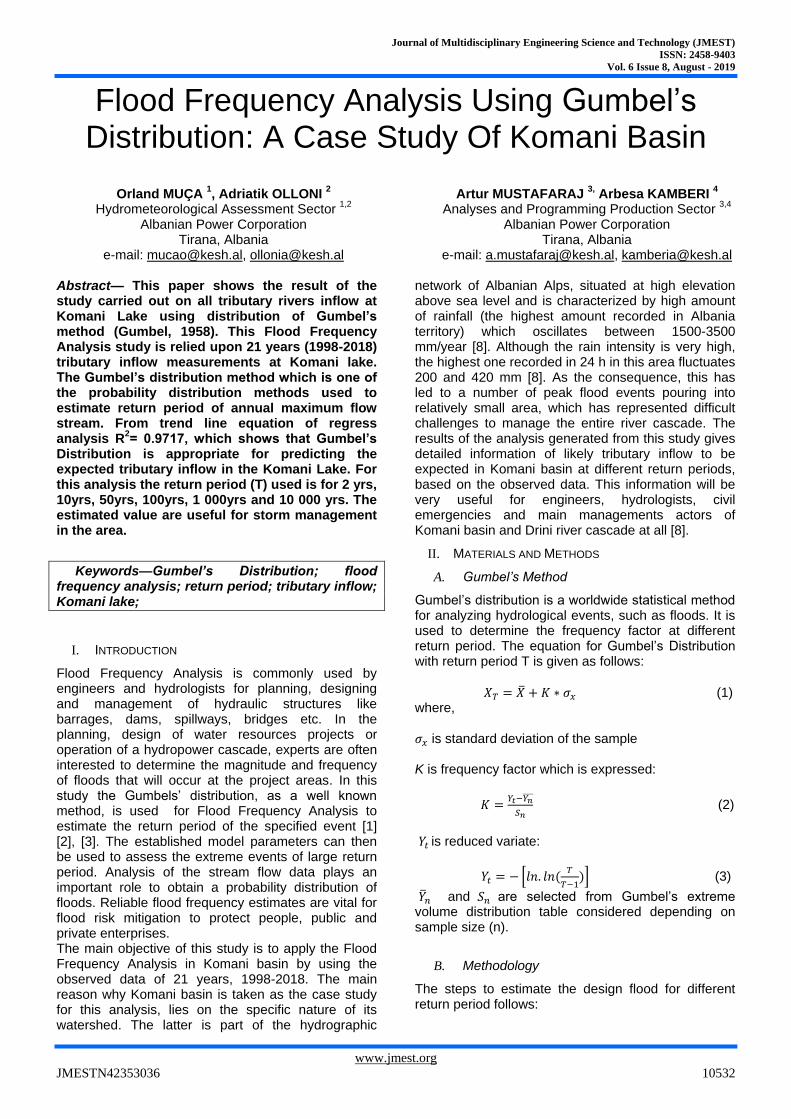
The case study taken in consideration all tributary inflow in Komani Lake. The Komani lake is part of Drini River cascade, which is managed by Albania Power Corporation, located in the north part of Albania, Western Balkan region. The watershed of study area lies within the boundaries between Komani HPP - Fierza HPP - Albanian Alps and Border of Kosovo as it is shown in figure 1; the watershed covers an area of approximately 1021 km
2. The inflow in the Komani lake
which comes from 2 main tributary rivers Valbona River and Shala River and from more than 7 small rivers. Part of the Komani inflow comes from Fierza HPP discharge (turbine and spillway). As such, artificial inflow has not been included in this study, therefore tributary inflow in Komani lake only is used as the main date for this analysis. Daily measurements are officially taken from Albanian Power Corporation owned stream gauges, which records hourly water
level of Komani lake used for calculation of hourly and daily tributary inflow.
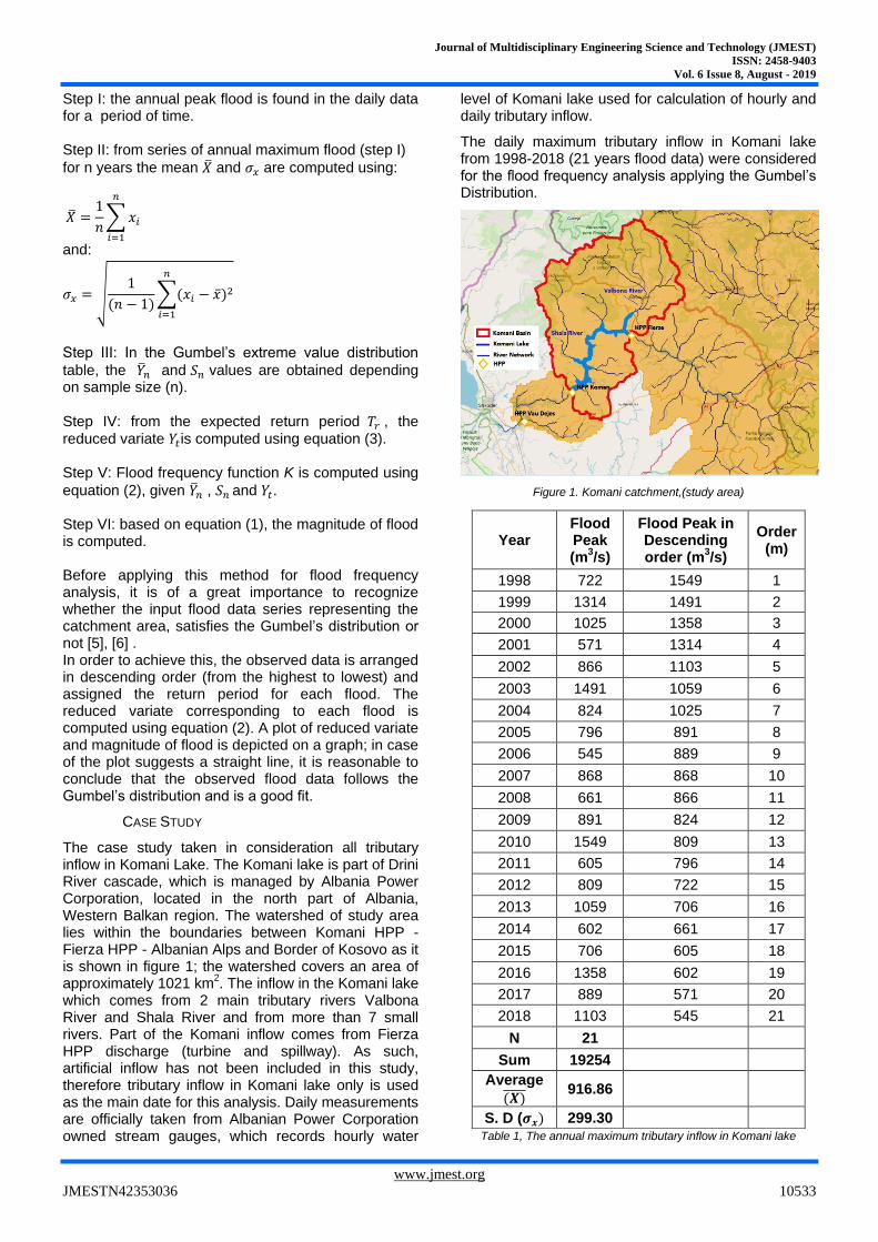
The daily maximum tributary inflow in Komani lake from 1998-2018 (21 years flood data) were considered for the flood frequency analysis applying the Gumbel’s Distribution.
Figure 1. Komani catchment,(study area)
Table 1, The annual maximum tributary inflow in Komani lake
Journal of Multidisciplinary Engineering Science and Technology (JMEST)
ISSN: 2458-9403
Vol. 6 Issue 8, August - 2019
www.jmest.org
JMESTN42353036 10534
Table 2. Computation table
Referred to Gumbel’s extreme value distribution table
For n = 21,
�̅�𝐧𝐢𝐬 𝟎. 𝟓𝟐𝟓𝟐
and
𝐒𝐧 is 1.0696.
S.D is Standard Deviation
III. RESULTS AND AND DISCUSSION
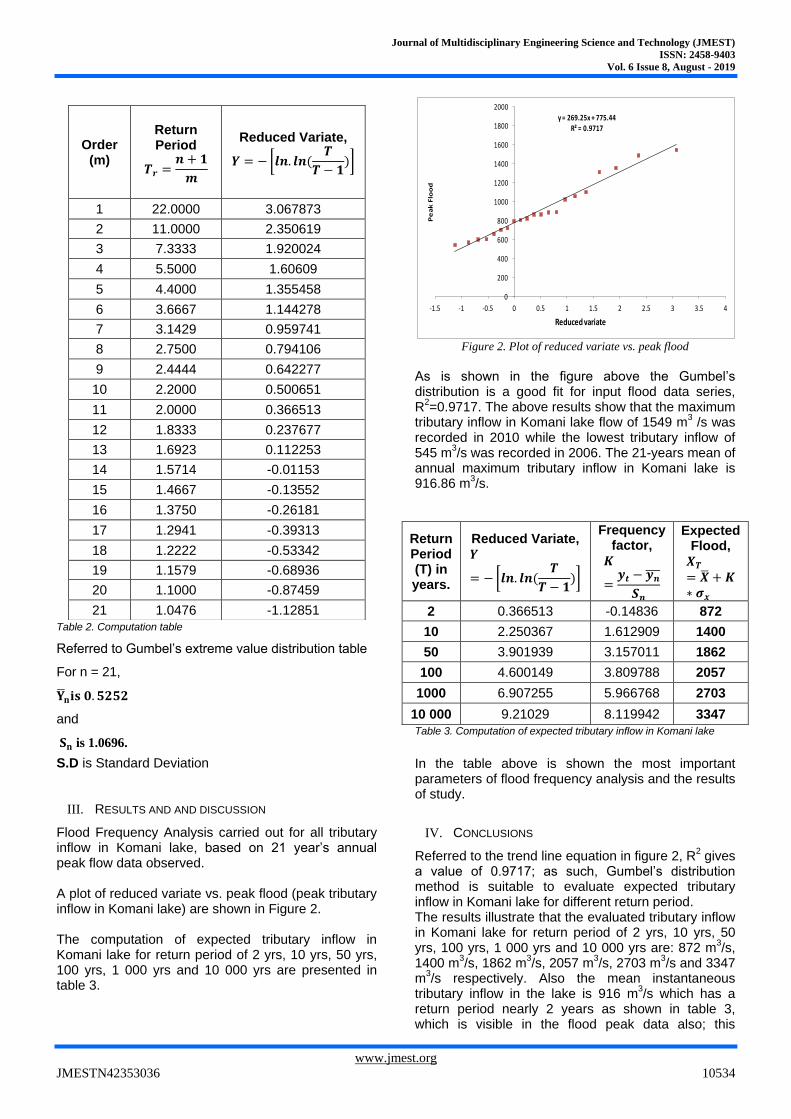
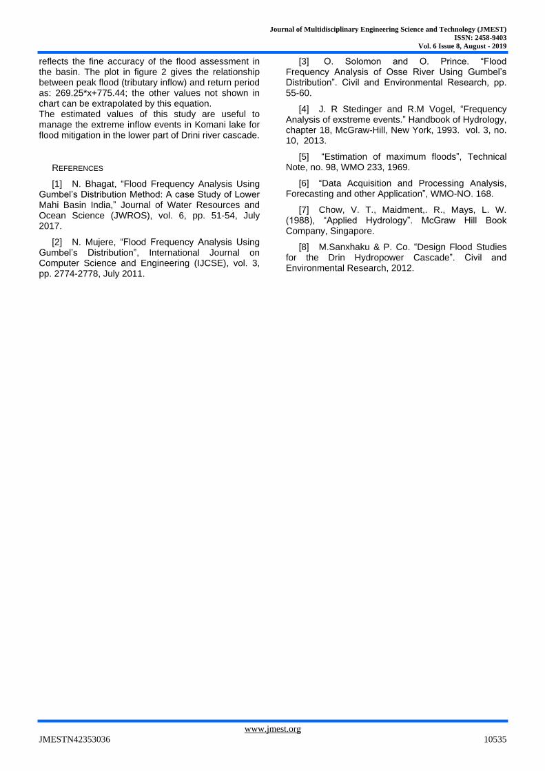
Flood Frequency Analysis carried out for all tributary inflow in Komani lake, based on 21 year’s annual peak flow data observed. A plot of reduced variate vs. peak flood (peak tributary inflow in Komani lake) are shown in Figure 2. The computation of expected tributary inflow in Komani lake for return period of 2 yrs, 10 yrs, 50 yrs, 100 yrs, 1 000 yrs and 10 000 yrs are presented in table 3.
Figure 2. Plot of reduced variate vs. peak flood
As is shown in the figure above the Gumbel’s distribution is a good fit for input flood data series, R
2=0.9717. The above results show that the maximum
tributary inflow in Komani lake flow of 1549 m3 /s was
recorded in 2010 while the lowest tributary inflow of 545 m
3/s was recorded in 2006. The 21-years mean of
annual maximum tributary inflow in Komani lake is 916.86 m
3/s.
Return Period (T) in years.
Reduced Variate, 𝒀
= − [𝒍𝒏. 𝒍𝒏 (𝑻
𝑻 − 𝟏)]
Frequency factor,
𝑲
=𝒚𝒕 − 𝒚𝒏̅̅ ̅
𝑺𝒏
Expected Flood,
𝑿𝑻
= �̅� + 𝑲∗ 𝝈𝒙
2 0.366513 -0.14836 872
10 2.250367 1.612909 1400
50 3.901939 3.157011 1862
100 4.600149 3.809788 2057
1000 6.907255 5.966768 2703
10 000 9.21029 8.119942 3347
Table 3. Computation of expected tributary inflow in Komani lake
In the table above is shown the most important parameters of flood frequency analysis and the results of study.
IV. CONCLUSIONS
Referred to the trend line equation in figure 2, R2 gives
a value of 0.9717; as such, Gumbel’s distribution method is suitable to evaluate expected tributary inflow in Komani lake for different return period. The results illustrate that the evaluated tributary inflow in Komani lake for return period of 2 yrs, 10 yrs, 50 yrs, 100 yrs, 1 000 yrs and 10 000 yrs are: 872 m
3/s,
1400 m3/s, 1862 m
3/s, 2057 m
3/s, 2703 m
3/s and 3347
m3/s respectively. Also the mean instantaneous
tributary inflow in the lake is 916 m3/s which has a
return period nearly 2 years as shown in table 3, which is visible in the flood peak data also; this
Journal of Multidisciplinary Engineering Science and Technology (JMEST)
ISSN: 2458-9403
Vol. 6 Issue 8, August - 2019
www.jmest.org
JMESTN42353036 10535
reflects the fine accuracy of the flood assessment in the basin. The plot in figure 2 gives the relationship between peak flood (tributary inflow) and return period as: 269.25*x+775.44; the other values not shown in chart can be extrapolated by this equation. The estimated values of this study are useful to manage the extreme inflow events in Komani lake for flood mitigation in the lower part of Drini river cascade.
REFERENCES
[1] N. Bhagat, “Flood Frequency Analysis Using Gumbel’s Distribution Method: A case Study of Lower Mahi Basin India,” Journal of Water Resources and Ocean Science (JWROS), vol. 6, pp. 51-54, July 2017.
[2] N. Mujere, “Flood Frequency Analysis Using Gumbel’s Distribution”, International Journal on Computer Science and Engineering (IJCSE), vol. 3, pp. 2774-2778, July 2011.
[3] O. Solomon and O. Prince. “Flood Frequency Analysis of Osse River Using Gumbel’s Distribution”. Civil and Environmental Research, pp. 55-60.
[4] J. R Stedinger and R.M Vogel, “Frequency Analysis of exstreme events.” Handbook of Hydrology, chapter 18, McGraw-Hill, New York, 1993. vol. 3, no. 10, 2013.
[5] “Estimation of maximum floods”, Technical Note, no. 98, WMO 233, 1969.
[6] “Data Acquisition and Processing Analysis, Forecasting and other Application”, WMO-NO. 168.
[7] Chow, V. T., Maidment,. R., Mays, L. W. (1988), “Applied Hydrology”. McGraw Hill Book Company, Singapore.
[8] M.Sanxhaku & P. Co. “Design Flood Studies for the Drin Hydropower Cascade”. Civil and Environmental Research, 2012.