Flood Routing Through Lake Nasser Using 2-D Model M...1-1 AIN SHAMS UNIVERSITY FACULTY OF...

1-1

AIN SHAMS UNIVERSITY

FACULTY OF ENGINEERING Irrigation and Hydraulics Department

Flood Routing Through Lake Nasser Using 2-D Model

A Thesis Submitted for Partial Fulfillment of the Requirements for the Degree of Doctorate of Philosophy in Civil Engineering

(Irrigation and Hydraulics) By

ASHRAF MOHAMED EL MOUSTAFA ABDEL BADIE

M.Sc. of Civil Engineering (Irrigation and Hydraulics)

Ain Shams University, 2002

Supervised By

Dr. Mohamed Abd Elhamid Gad Lecturer, Irrigation and Hydraulics Department Faculty of Engineering Ain Shams University

Cairo 2007

Prof. Dr. MOUSTAF M. SOLIMAN Professor of Irrigation Engineering Irrigation and Hydraulics Department Faculty of Engineering Ain Shams University

Prof. Dr. Mohamed Bahaa El Deen Head of the Irrigation Sector, Irrigation and Water Resources Vise Minister, Ministry of Irrigation and Water Resources

Chapter one Introduction

1-2


1-3

CHAPTER ONE

Introduction 1.1 General

High Aswan Dam (HAD) construction was completed in 1968 providing

full control on the discharges released to the Egyptian irrigation network

system. This resulted in the formation of a reservoir that trapped almost

all of the inflow and hence formed a large reservoir. The High Aswan

Dam Reservoir (HADR) extends for 500 km along the Nile River and

covers an area of 6,000 km2 at water level equal 182.00 m above mean

sea level.

An uncontrolled spillway was constructed at the end of Khor Tushka (on

the western side of Lake Nasser at about 256 km upstream the dam). This

spillway is connected to Tushka depression by a canal by which the

excess flood can be turned to the depression.

1.2 Scope of Work

The question of operation of the HAD was neglected for a long time after

the dam has been constructed as it seemed simple as the inflows were

large enough so the water could always be released to meet downstream

requirements and any water remaining was simply used to fill the

reservoir behind the dam.

The ministry of irrigation currently decides the daily release from the

HAD, and the ministry of electricity determines the distribution of

discharges over the 24 hour period in order to effectively integrate the

hydroelectric generation into the daily requirements of the national grid.


1-4

The development of river basin policy and management plans involves a

spectrum of concerned parties and organizations, only a small fraction of

which are presented by technical professionals. Easily-used and highly-

interactive computer simulations provide one means by which these

individuals can develop a conceptual and intuitive understanding for the

complex physical behavior of river systems.

The thesis presents the development of a 2D simulation model of HADR.

The modeling study aims to determine the optimal management policy

for the reservoir in flood conditions by modeling the physical problem

via a 2D routing model. The hydrodynamic model simulated the flow

fields – steady and unsteady- of the High Aswan Dam Reservoir.

During the work progress a hydrological model, HADR Simulator, was

developed for dam operation as the hydrodynamic model generated was

useful in future studies of sedimentation or water quality but found to be

time consuming if it to be used for dam operation.

1.3 Organization of Work

This thesis is organized in eight chapters as follows to study to what

extend the spillway will protect HAD against floods with levels more

than the maximum design levels.

Chapter one: gives an introduction about the subject and the

organization of the work and objectives.

Chapter two: presents brief notes and literature review about routing

techniques, hydrodynamic and hydrological methods, which were used in

the development of thesis models.


1-5

Chapter three: presents the problem definition, description of High

Aswan Dam Reservoir and scope of the thesis.

Chapter four: presents the data preprocessing and the simulation of a of

the reservoir bed level with a three dimensional surface.

Chapter five: presents the model selection, description and limitations.

The development of the two-dimensional hydrodynamic model,

calibration and verification process, steady state simulations are also

presented.

Chapter six: presents the study of various flood waves and the real flood

wave on the developed model and the modifications made to the

hydrodynamic model to be used in the dam operation.

Chapter seven: presents the development of hydrological model for the

purpose of dam operation along with the results of testing the effect of

varying the model parameters.

Chapter eight: presents the main conclusion of the research and also

states the recommendations to be taken into consideration in the future

work.


1-6

1.1 General ..................................................................................... 3 1.2 Scope of Work ........................................................................... 3 1.3 Organization of Work ................................................................. 4


1-7

CHAPTER TWO

Literature Review

General

This chapter describes several different hydraulic and hydrologic routing

techniques. Assumptions, limitations, data requirements for each and the

basis for selection of a particular routing technique are reviewed.

Routing is a process used to predict the temporal and spatial variations of

a flood hydrograph as it moves through a river reach or reservoir. The

effects of storage and flow resistance within a river reach are reflected by

changes in hydrograph shape and timing, attenuation and travel time, as

the floodwave moves from upstream to downstream. In general, routing

techniques may be classified into two categories: hydraulic routing, and

hydrologic routing.

Hydrologic Versus Hydraulic Routing Techniques

The hydrologic method is in general simpler but fails to give entirely

satisfactory results in problems other than of determining the progress of

a flood down a long river. For example when a flood comes through a

junction, backwater is usually produced and this can only be accurately

evaluated by the basic hydraulic equations.

Hydraulic routing techniques are based on the solution of the partial

differential equations of unsteady flow. Hydrologic routing employs the

continuity equation and an analytical or an empirical relationship

between storage within the reach and discharge at the outlet.


1-8

The hydrologic approaches, which are simpler to use but harder to defend

theoretically, on the other hand the hydraulic approaches, which are

better grounded in basic theory are relatively difficult to apply. It is the

relationship between the geometrical quantity, storage, and the kinematic

quantities, discharge hydrographs, which makes the hydrologic and

hydraulic approaches differ.

In channel design, floodplain studies, and watershed simulations,

generally, hydrologic routing is utilized on a reach-by-reach basis from

upstream to downstream. This type of approach is adequate as long as

there are no significant backwater effects or discontinuities in the water

surface because of jumps or bores.

When there are downstream controls that will have an effect on the

routing process through an upstream reach, the channel configuration

should be treated as one continuous system. This can only be

accomplished with a hydraulic routing technique that can incorporate

backwater effects as well as internal boundary conditions, such as those

associated with culverts, bridges and weirs.

It is possible that the transverse variations will be of greater importance

than the stream wise values. This is why we used a 2D model in our

study due to the natural sophisticated lay out of the HAD reservoir.


1-9

Hydraulic Routing Technique

The equations that describe the unsteady flow in the three dimensions,

the Saint Venant equations, consist of the conservation of mass equation,

Equation 2-1, and the conservation of momentum equation, Equation 2-2.

The solution of these equations defines the propagation of a flood wave

with respect to distance along the channel and time.

0

z

w

y

v

x

u (2-1)

0)()()(

xxzxyxx x

p

z

u

zy

u

yx

u

xz

uw

y

uv

x

uu

t

u

0)()()(

yyzyyyx y

p

z

v

zy

v

yx

v

xz

vw

y

vv

x

vu

t

v

0)()()(

zzzzyzx z

p

z

w

zy

w

yx

w

xz

ww

y

wv

x

wu

t

w

(2-2)

where

u = average velocity of water in x direction;

x = distance along channel in x direction;

v = average velocity of water in y direction;

y = distance along channel in y direction;

w = average velocity of water in z direction;

z = distance along channel in z direction;

ρ = water density;

τ = shear stress;

t = time;


1-10

ε = Eddy viscosity;

Solved together with the proper boundary conditions, Equations 2-1 and

2-2 are the complete dynamic wave equations. The dynamic wave

equations are considered to be the most accurate and comprehensive

solution to 1-D unsteady flow problems in open channels.

The full unsteady flow equations have the capability to simulate the

widest range of flow situations and channel characteristics. Hydraulic

models, in general, are more physically based since they only have one

parameter (the roughness coefficient) to estimate or calibrate. Roughness

coefficients can be estimated with some degree of accuracy from

inspection of the waterway, which makes the hydraulic methods more

applicable to ungauged situations. Hydrologic Routing Technique Hydrologic routing employs the use of the continuity equation and either

an analytical or an empirical relation ship between storage within the

reach and discharge at the outlet. In its simplest form, the continuity

equation can be written as inflow minus outflow equals the rate of

change of storage within the reach:

I – O = t

S

(2-3)

Where

I = the average inflow to the reach during Δt,

O = the average outflow from the reach during Δt and

S = storage within the reach [L3].

Additional terms can be added to this formula according to its importance

and the avaliable data for calculation. One of those important terms in the


1-11

study of great reservoirs with large surface area is the evaporation factor

which acts as an outflow from the reservoirs but in an upword direction,

also precipitation can be considered as the evaporation with a negative

sign. Bank storage and groundwater-lake interaction are also two

important factors that may be considered specially for reservoirs and big

rivers.

Some of the famous hydrological routing techniques are summarized

below.

1. Modified Puls Reservoir Routing.

The equation defining storage routing, based on the principle of

conservation of mass, can be written in approximate form for a routing

interval t . Assuming the subscripts “1” and “2” denote the beginning

and end of the routing interval, the equation is written as follows:

t

SSIIOO

122121

22 (2-4)

2. Modified Puls Channel Routing.

Routing in natural rivers is complicated by the fact that storage in a river

reach is not a function of outflow alone. During the passing of a flood

wave, the water surface in a channel is not uniform. The storage and

water surface slope within a river reach, for a given outflow, is greater

during the rising stage of a flood wave than during the falling stage.

Therefore, the relationship between storage and discharge at the outlet of

a channel is not a unique relationship, rather it is a looped relationship.

3. Muskingum Method.

The Muskingum method was developed to directly accommodate the

looped relation-ship between storage and outflow that exists in rivers.


1-12

With the Muskingum method, storage within a reach is visualized in two

parts: prism storage and wedge storage. Prism storage is essentially the

storage under the steady-flow water surface profile. Wedge storage is the

additional storage under the actual water surface profile. During the

rising stages of the flood wave, the wedge storage is positive and added

to the prism storage. During the falling stages of a flood wave, the wedge

storage is negative and subtracted from the prism storage.

S = prism storage + wedge storage

S = KO + KX (I - O)

S = K [XI + (1 - X)O] (2-5)

Where

S = total storage in the routing reach;

O = rate of outflow from the routing reach;

I = rate of inflow to the routing reach;

K = travel time of the flood wave through the reach;and

X = dimensionless weighting factor, ranging from 0.0 to 0.5

4. Working R & D Routing Method.

This method is also useful in situations wherein the horizontal

reservoir surface assumption of the modified puls procedure is

not applicable, such as normally occurs in natural channels.

The working R&D procedure could be termed “Muskingum with a

variable K” or “modified puls with wedge storage.” For a straight line

storage-discharge (weighted discharge) relation, the procedure is the

same solution as the Muskingum method. For X = 0, the procedure is

identical to Modified Puls.


1-13

Typically, in rainfall-runoff analysis, hydrologic routing procedures are

utilized on a reach-by-reach basis from upstream to downstream. In

general, the main goal of the rainfall-runoff study is to calculate

discharge hydrographs at several locations in the watershed. In the

absence of significant back water effects, the hydrologic routing models

offer the advantages of simplicity, ease of use, and computational

efficiency .

Also, the accuracy of hydrologic methods in calculating discharge

hydrographs is normally well within the range of acceptable values. It

should be remembered, however, that insignificant backwater effects

alone do not always justify the use of a hydrologic method. There are

many other factors that must be considered when deciding if a hydrologic

model will be appropriate, or if it is necessary to use a more detailed

hydraulic model.


1-14

Evaluating The Routing Method With such a wide range of hydraulic and hydrologic routing techniques,

selecting the appropriate routing method for each specific problem is not

clearly defined. However, certain thought processes and some general

guidelines can be used to narrow the choices, and ultimately the selection

of an appropriate method can be made.

There are several factors that should be considered when evaluating

which routing method is the most appropriate for a given situation. The

following is a list of the major factors that should be considered in this

selection process:

1. Backwater effect.

2. Flood plains.

3. Channel slope and hydrograph characteristics.

4. Flow networks.

5. Flow regiem.

6. Data availability.

Steady versus Unsteady Flow Models The traditional approach to river modeling has been the use of hydrologic

routing to determine discharge and steady flow analysis to compute water

surface profiles. This method is a simplification of true river hydraulics,

which is more correctly represented by unsteady flow. Nevertheless, the

traditional analysis provides adequate answers in many cases.

Steady flow analysis is defined as a combination of a hydrologic

technique to identify the maximum flows at locations of interest in a

study reach (termed a "flow profile") and a steady flow analysis to

compute the (assumed) associated maximum water surface profile.


1-15

Steady flow analysis assumes that, although the flow is steady, it can

vary in space. In contrast, unsteady flow analysis assumes that flow can

change with both time and space.

Unsteady flow analysis should be used for all streams where the slope is

less than 2 feet per mile. On these streams, the loop effect is predominant

and peak stage does not coincide with peak flow. Backwater affects the

outflow from tributaries and storage or flow dynamics may strongly

attenuate flow; thus, the profile of maximum flow may be difficult to

determine.

Previous Studies Several studies were done on the flood routing technequies, flood routing

modelling and dam operation models some of these studies are presented

as follows.

M. S.K. Chowdhury and F. C. Bell (1980) developed a new runoff

routing model that combines realistic allowances for the spatial

distribution of storage with the theoretically satisfying features of the

kinematic wave approximation. Appropriate boundary conditions enabled

replacement of the partial differential equations describing the flow by

tractable total differential equations.

In addition, similar forms of equations have been adopted to describe

both overland and channel flow. All these features resulted in a relatively

simple model with a small number of physically relevant parameters that

are not difficult to evaluate.

The required model input is a temporal pattern of rainfall excess from a

runoff generation model. A number of quite different runoff generating

models may all be used for this purpose. However, the estimation of


1-16

rainfall excess will not be considered here, since the focus of this paper is

on the development of the new routing procedure.

The use of the current discharge as a state variable enables the model to

be automatically tuned to the current conditions and is particularly

suitable for short-term flood forecasting.

Bernard L. Golding (1981) developed a Basic language program for

routing floods through storage reservoirs or detention basins by the

storage-indication working curve method (Modified Plus Method). A

sample program was included and explained step-by-step. Standard flood

routing equations were included. Many municipalities require that post-

development runoff cannot exceed pre-development runoff in their

subdivision regulations. Building a retention basin that acts as a small

flood control reservoir normally did this.

Stanley S. Butler (1982) presented an alternate reservoir flood routing

approach applicable for routing design floods determined from

statistically derived design storms. The approach treated routing as an

instantaneous discharge point-function process instead of an average

discharge incremental time procedure, avoiding some of the difficulties

and errors in the traditional methods.

The point-slope method of routing floods through reservoirs used in his

work can be described as follows. He used instantaneous-time functions

in the form of equations for determining the outflow hydrograph slope

and the inflection point of the rising limb of the outflow hydrograph

based on the inflow hydrograph, the topography of the reservoir, and the

hydraulic characteristics of the outflow structure.

The point-slope method is less broadly applicable than the traditional

incremental-time methods, but within its limitations (simple single-


1-17

peaked inflow hydrographs), it is fast, accurate, and adaptable for

investigating alternate designs. A check and adjustment procedure

provides assurance that the result is valid. This procedure and the criteria

for determining the inflection point of the outflow hydrograph are of

general applicability with reservoir flood routing methods.

Richard J. Heggen (1983) developed a Basic program to route flood

discharge through a system of river channels and reservoirs. The brevity

of this program and the use of an overlaid computational matrix make it

suitable for minicomputer execution.

Channel hydrographs are computed by the Muskingum method; reservoir

hydrographs, by the Puls method. Data input consists of routing

coefficients for channels, reservoir state-discharge-storage curves, and

description of network configuration. The program is suited for analysis

of open channels conveyance systems, flood detention reservoirs and

combination of two.

Tawatchai Tingsanchali and Shyam K. Manandhar (1985) developed

an analytical diffusion model for flood routing, the basic diffusion

equation is linearized about an average depth and takes into account

backwater effect and lateral flows. The model was applied to route the

floods in a hypothetical rectangular channel with different upstream,

downstream, and lateral boundary conditions.

The applicability of the model is limited to slow rising floods in which

the effects of flow acceleration can be neglected. The channel

characteristics were assumed and the results obtained were compared

with those obtained by the finite difference method of implicit scheme

based on the complete Saint-Venant equations for unsteady open channel

flow and were found to have a standard deviation of about 0.035.


1-18

The model showed good results when applied to simulate flood flow

conditions in 1980 and 1981 in the Lower Mun River, in Northeast

Thailand. The model cannot be incorporated with detailed data of cross

sections or riverbed geometry. It only requires only their average values.

The Chézy, C and the diffusivity, k due to channel irregularities were

used in the model and were determined by trial and error during model

calibration. The model provides an excellent means to analyze individual

or overall effects of the boundary conditions and requires much less

effort and time for computation at a particular station.

D.L. Fread, National weather service (NWS) (1988) developed the

Hydrologic Research Laboratory (HRL) of the NWS Office of

Hydrology dynamic wave routing models suitable for efficient

operational use in a wide variety of applications involving the prediction

of unsteady flows in rivers, reservoirs, and estuaries. These models are

based on an implicit (four-point, nonlinear) finite-difference solution of

the complete one-dimensional Saint-Venant equations of unsteady flow.

Because, fixed arrays within the computer program for the number of

time steps and number of cross sections severely limit the size of the

river systems that can be modeled without breaking up the application

into several datasets. Since the mid-1980's, a comprehensive Flood Wave

routing model (FLDWAV) has been undergoing development and

testing. This state of the art model combines the capabilities of

DWOPER and DAMBRK, and provides features not contained in either

of these models.

FLDWAV has undergone extensive testing (over 160 datasets) to ensure

The same level of accuracy and stability as the DAMBRK and DWOPER

models. It has also gone through two years of beta testing. The

FLDWAV model will continue to undergo development improvements


1-19

and testing by the NWS to increase its range of applicability and

numerical robustness for more convenient usage.

FLDWAV is a generalized flood routing (unsteady flow simulation)

model. The governing equations of the model are the complete one-

dimensional Saint-Venant equations of unsteady flow, which are coupled

with internal boundary equations representing the rapidly varied (broad-

crested weir) flow through structures such as dams, and bridge

embankments, which can develop a user, specified time-dependent

breach. In addition, appropriate external boundary equations at the

upstream and downstream ends of the routing reach are utilized.

The system of equations is solved by an iterative, nonlinear, weighted

four-point implicit finite-difference method. The flow may be either

subcritical or supercritical or a combination of each varying in space and

time from one to the other; fluid properties may obey either the principles

of Newtonian (water) flow or non-Newtonian (mud/debris flows or the

contents of a mine-tailings dam) flow. The hydrograph to be routed may

be user-specified as an input time series, or it can be developed by the

model via user-specified breach parameters (size, shape, time of

development).

The possible presence of downstream dams, which control the flow and

may be breached by the flood, bridge/embankment flow constrictions,

tributary inflows, river sinuosity, levees located along the tributaries

and/or downstream river, and tidal effects are each properly considered

during the downstream propagation of the flood.

H. A. Basha (1995) developed a routing equation for detention reservoir

systems from an approximate analytical solution of the nonlinear storage

differential equation. The approximate solution was obtained by a two-

term perturbation expansion whereby the zeroth-order term is the linear


1-20

solution and the first-order term is the correction. The first-order

approximation, which allows for arbitrary multi-event inflow

hydrographs, irregular reservoir configuration, and various types and

sizes of outlets, is found to be accurate for all practical purposes. The

asymptotic solution allowed the derivation of design equations that can

apply for arbitrary reservoir configuration and for various types and sizes

of outlet.

Tefaruk Haktanir and Hatice Ozmen (1997) computed, using the

computer program DUFLOW package, the Outflow hydrographs for

three dams with long lakes in narrow valleys using both hydrologic

routing (level-pool routing) and hydraulic routing. These hydrographs

were then compared with three inflow hydrographs of different peaks.

The DUFLOW package is based on the one-dimensional partial

differential equations to describe unsteady flow in open channels, the

continuity and momentum equations.

In all these cases, the difference between outflow hydrographs was

greatest at the peak value relative to the magnitude of the inflow

hydrograph. The peak outflow by hydraulic routing was smaller than that

by hydrologic routing for all the routing combinations, the difference

varying between 2 and 11%.

Francisco Nunes Correia et al (1998) presented results based on the use

of Intergraph GIS coupled with Idrisi GIS. Using these two systems

substantially increased the flexibility of using GIS as a tool for flood

studies.

A lumped (XSRAIN) and a distributed (OMEGA) hydrologic model

were used to simulate flood hydrographs. The well known HEC-2

Hydraulic model was used to compute flooded areas. These models were

applied in the Livramento catchment with very good results. The

computation of flooded areas for different flood scenarios, and its


1-21

representation in GIS, can be used in the assessment of affected property

and associated damages.

This is a very useful GIS-based approach to floodplain management.

Geographic Information Systems (GIS) have been recognized as a

powerful means to integrate and analyze data from various sources in the

context of comprehensive floodplain management. As part of this

comprehensive approach to floodplain management, it is very important

to be able to predict the consequences of different scenarios in terms of

flooded areas and associated risk.

Hydrologic and hydraulic modeling plays a crucial role and there is much

to gain in incorporating these modeling capabilities in GIS. This is still a

rather complex task and research to be made on the full integration of

these models. Interfacing between these models and GIS may be a very

efficient way of overcoming the difficulties and getting very good results

in terms of engineering practice.

T. R. Neelakantan and N. V. Pundarikanthan (2000) trained a back

propagation neural network to approximate the simulation model

developed for the Chennai city water supply problem. The neural

network was used as a sub-model in a Hooke and Jeeves nonlinear

programming model to find ‘‘near optimal policies.’’

The results were further refined using the conventional simulation-

optimization model. There have been several attempts to use combined

simulation-optimization models to solve reservoir operation problems

efficiently. In many cases, complex simulation models are available, but

direct incorporation of them into an optimization framework is

computationally prohibitive, this is why this model was developed.


1-22

Abbas Seifi and Keith W. Hipel (2001) proposed a new method for

long-term reservoir operation planning with stochastic inflows. In

particular, the problem was formulated as a two-stage stochastic linear

program with simple recourse. Multiple inflow scenarios, leading to a

very large deterministic model that is hard to solve using conventional

optimization methods, approximated the stochastic inflows. An efficient

interior-point optimization algorithm was presented for solving the

resulting deterministic problem. It was also shown how exploiting the

problem structure enhances the performance of the algorithm.

Application to regulation of the Great Lakes system shows that the

proposed approach could handle the stochastic of the inflows as well as

the nonlinearity of the operating conditions in a real-world reservoir

system.

Mohamed M. Hantush, Morihiro Harada and Miguel A. Marin

(2002) Analytical solutions were developed for routing stream flow,

lateral stream-aquifer interactions, and aquifer storage. In effect, the

stream- flow routing Muskingum method was modified for bank storage.

The analysis was based on one-dimensional lateral groundwater flow in

semi-infinite homogeneous unconfined aquifers, which are in contact

with streams through semi-pervious bed sediments.

Impulse response and unit step response functions were derived for the

stream-aquifer system, using Laplace transformations. These response

functions relate stream outflow, stream-aquifer flow, bank storage, and

cumulative reach discharge volume to discrete-time inflow hydrographs

through convolution integrals.

The impulse response function decreases with increasing aquifer

hydraulic conductivity at earlier times, but increases with the

conductivity and persists at later times. The unit step response function

decreases with aquifer conductivity uniformly in time. The dependence


1-23

of stream flow and bank storage on aquifer hydraulic conductivity,

streambed leakage, stream width, and aquifer diffusivity was

investigated. The analysis was extended to discrete input data, and

modification of the methodology to route discrete-time inflow

hydrographs of general form was achieved, using discrete-time kernels.

The presented analysis establishes the time domain for validity of the

analytical solutions in terms of the Muskingum parameters and an

aquifer-related parameter.

Francisco J. Rueda and S. Geoffrey Schladow (2003) examined the

internal dynamics of Clear Lake, California-a large, multibasin and

polymictic lake-were using simulations conducted with a three-

dimensional hydrodynamic model. The model was based on an accurate

and efficient semi-implicit finite difference algorithm for the

hydrodynamic equations, which has been previously subject to extensive

verification with analytical test cases.

The high level of agreement-without extensive calibration-between the

model results and the observations at several locations in the lake is

comparable with previously published 3D modeling results. The model

results confirmed the baroclinic-pumping model of circulation proposed

for the Oaks Arm of Clear Lake.

The simulations showed that the interaction of stratification, periodic

wind forcing, and Coriolis effects drive this circulation. The diurnal

readjustment of the circulation from being wind driven to baroclinically

driven was examined and shown to vary spatially. This transition in

circulation-type has a wavelike nature, with a distinct frontal structure

and converging currents at the surface. Asymmetries in the forcing and

response, combined with rotational effects, impart a cyclonic residual

circulation on the flow.


1-24

M. El-Moattassem et al (2003) developed an approach for simulating

the flow of water in High Aswan Dam Reservoir (HADR) and for

predicting the sediment transport and determine solutions to overcome

the problems associated with the sediment deposition.

The Surface Water Modeling System (SMS) were used for the study.

During a simulated flood event, RMA2 computes a time-history of water

depth and depth-averaged velocity at each node in the mesh. These data

are used by SED2D to compute a bed shear stress. SED2D compares the

bed shear stress with the measured or estimated physical properties of the

bed material to compute the sediment transport rate and cumulative scour

or deposition at each node of the mesh in the study area.

Luis F. León et al (2004) evaluated the predictive capability of the 3-D

Estuary and Lake Computer Model (ELCOM) using relatively high

quality data collected on Great Slave Lake - one of the largest lakes of

the world in Canada’s northern climatic system. This assessment is an

important step in the ongoing research to develop a coupled lake-

atmosphere model - a major consideration in the development and testing

of the lake model.

A validation run was performed with 2003 data in the Great Slave Lake.

Vertical thermistor chain data was compared against model calculations

and mean circulation patterns were presented. Comparison runs were

made with meteorological field data and with output from a Regional

Climate Model (RCM) as input to the hydrodynamic model to determine

the differences in forcing data affecting simulations of surface

temperature and circulation.

Richard O. Anyah, Fredrick Semazzi and Lian Xie (2006)

Thermodynamic and hydrodynamic characteristics of Lake Victoria are

investigated based on idealized simulations using a 3D-lake model. A


1-25

suite of simulations with an elliptic (oval) geometry and prescribed wind

speed (surface wind stress), lake-atmosphere temperature difference and

vertical temperature profile were performed.

The time evolutions of lake temperature as well as the currents

(circulation characteristics) at different depths and/or points are analyzed

in order to understand the lake’s response to certain aspects of surface

forcing conditions. Similarities and differences between the features

simulated in a typical tropical lake (Lake Victoria) and typical mid-

latitude lake(s) based on the effects of the Coriolis force are also

examined.

The simulations revealed a number of unique features in the temperature.

Considered at different points on the lake surface, the temperature of

both runs with or without effect of Coriolis force equilibrates after almost

the same time (between 30-40 days). However, there is a conspicuous

difference in the vertical temperature profiles of the two runs (cases). For

example, the MIDLAT run is characterized by a ‘dome-shaped’ profile in

the bottom layers (40m and deeper) after 30 days of model integration, in

contrast to the VICTORIA case which is nearly isothermal over the full

water column.

Perhaps one of the most significant outcomes of the presented study is

that the two-gyre circulation pattern shown in the VICTORIA case after

30 days of model integration is also present in the simulations with

observed lake bathymetry.


1-26

Conclusion

From the previous studies it was found that it is necessary to develop a

two dimensional model to simulate the various flow fields, steady and

unsteady of the High Aswan Dam Reservoir. Then use this model in the

reservoir management and dam operation. Taking into account the water

strategy followed by the Egyptian ministry of Irrigation. Which states

that when handling the flood discharges the flood year starts with water

level of 175.00 m upstream HAD and considering the presence of Tushka

side spillway which begins to discharge water to Tushka depression

through Tushka canal when water level reaches (178.00) which was built

for the safety of the HAD. In addition, it is important to put different

scenarios when dealing with flood or drought years.


1-27

2.1 General ................................................................................................. 7 2.2 Hydrologic Versus Hydraulic Routing Techniques ............................. 7 2.3 Hydraulic Routing Technique .............................................................. 9 2.4 Hydrologic Routing Technique ......................................................... 10 2.5 Evaluating The Routing Method ....................................................... 14 2.6 Steady versus Unsteady Flow Models ............................................... 14 2.7 Previous Studies ................................................................................. 15 2.8 Conclusion ......................................................................................... 26


1-28

CHAPTER THREE

The Problem Definition

3.1 River Nile

The Nile has played an important part in the cultural history of the world

and in the development of great civilizations. While still in the areas from

which its waters flow, the water runs unregulated and uncontrolled

putting people at the mercy of floods and slack periods.

This is not a matter which affects one country or two but the whole Nile

countries are concerned and involved. If all the countries affected by the

Nile waters cooperate to control this great force and use it for the benefit

of all their peoples, they can make great advances. (Fahmy and El

Shibini, 1979).

3.2 High Aswan Dam (HAD)

The HAD is located 6.500 km upstream the old Aswan dam, about 950

km South of Cairo. It is 3600 meters long along the top and has a

maximum height of 111 meters. The width of the base is 980 meters. 43

million cubic meter of materials were used in its construction, the

structure is seventeen times larger than the Great Pyramid of Giza.

The operation of the HAD is the responsibility of the High Aswan Dam

Authority (HADA), whose chairman reports directly to the minister of

Irrigation. The High Aswan Dam is the most famous dam in the world, and the

management of such dam is not a problem which will be finally solved


1-29

and then left to technocrats to implement. The policy for managing this

dam will evolve over time as new water resources problems emerge.


1-30

3.3 High Aswan Dam Reservoir (HADR)

The construction of High Aswan Dam (HAD) in Upper Egypt resulted in

the formation of a reservoir that trapped almost all of the inflow and

hence forms a large reservoir.

The length of HAD reservoir is about 500 km with an average width of

about 12 km and a surface area of 6540 km2 at its maximum storage

level. Which is (182.00) m. This reservoir is considered to be the second

largest man-made lake in the world, where the storage capacity of the

reservoir has a volume of 162 billion m3 allocated as follows:

(1) 31 billion m3 for dead storage (which corresponds to a lake level

of 147 meters above sea level).

(2) 90 billion m3 for live storage (which corresponds to a lake level

up to 175 meters above sea level).

(3) 41 billion m3 for flood protection (which corresponds to a lake

level of 182 meters above sea level).

3.4 Tushka Canal Project As Lake Nasser reached its operating range, the ministry of irrigation

became concerned about the ability of the reservoir to handle a high

flood without causing scouring damages of the main channel, barrages

and other structures across the Nile main stream.

Tushka project was proposed by the ministry of irrigation to effectively

create a safety valve to remove excess water from the HADR by cutting a

canal from the western edge of the reservoir north of Abo Smpel through

the Western desert to the Tushka depression, where it would empty

harmlessly into barren desert.


1-31

The canal was initially designed to be 350 meters wide with a capacity of

365 million m3 per day and to run for 22 km until it empties into Tushka

depression. The first phase of the project called for an unregulated

spillway at 178 meters above sea level at the canal entrance. (Several

studies were carried out to replace such spillway with a controlled

structure).

3.5 Problem Identification

The question of operation of the HAD was neglected for a long time after

the dam has been constructed as it seemed simple as the inflows were

large enough so the water could always be released to meet downstream

requirements and any water remaining was simply used to fill the

reservoir behind the dam. In the last decay, many researches related to

the management of the dam were carried out within the HADA and in

some of the ministry's water research centers.

The purpose of any reservoir is to regulate the fluctuations in a river's

discharge in order to obtain a more desirable pattern of flows. However,

the operating policies differ between reservoirs for three reasons:

(1) The structure of the dam and the physical characteristics of the

reservoir's behavior vary in different locations.

(2) The statistical characteristics of flows vary in different rivers.

(3) The value of different levels of achievements of the objectives to

the economic and political systems varies in different locations.

The ministry of irrigation currently decides the daily release from the

HAD, and the ministry of electricity determines the distribution of

discharges over the 24 hour period in order to effectively integrate the

hydroelectric generation into the daily requirements of the national grid.


1-32

The release of great amount of water from the HAD may result in some

degradation. So one of the objectives of the reservoir management is find

a pattern of releases which would result in an acceptable level of

degradation. The ministry of irrigation also requires that the daily

discharges be limited to 250 million m3 per day in order to avoid

damages to the river channel and barrages.

One of the most important projects which are carried out by the ministry

of irrigation is the replacement of the great barrages on the Nile in order

to increase the maximum daily release of the HAD to help in the

agriculture area extending projects in Egypt.

Currently, the management policy of the reservoir, to handle high floods,

is to lower the water level by the end of July, that is the beginning time of

the year flood, to at least (175.00) m. In order for the reservoir to have

the capacity to store the peak of a high flood, the entire incoming flood

and all the subsequent inflows of the water year minus the evaporation

and seepage losses must be released over a twelve month period in order

to bring the water level back to 175 meters by the following end of July.

If a higher level than 175 meters is used, more water is stored as

insurance against a series of low years, the head on the turbines is higher,

evaporation losses are greater, but the risk of damages from a high flood

is increased.


1-33

3.6 Scope of the Thesis The Scope of the thesis can be summarized into the following points:

1. Development of a bathymetry (3 dimensioned bed level profile)

of the High Aswan Dam Reservoir from the upstream about 460

kilometers HAD and ending just upstream the dam. This

bathymetry will be used to interpolate the levels of mesh points

used during the modeling process.

2. Development of a 2 dimensional hydrodynamic model as the first

hydrodynamic model for the reservoir. This model is the first

step for sediment transport studies and water quality studies of

the lake.

3. Study of the water surface profiles variation with respect to

different flow rates, flood wave slopes and initial water level in

the reservoir.

4. Study of real flood wave movement through the reservoir.

5. Development of an operating model for the High Aswan Dam

releases.


1-34

3.1 River Nile ........................................................................................... 28 3.2 High Aswan Dam (HAD) .................................................................. 28 3.4 Tushka Canal Project ......................................................................... 30 3.5 Problem Identification ....................................................................... 31 3.6 Scope of the Thesis ............................................................................ 33


1-35

CHAPTER FOUR

Data Preprocessing 4.1 Data Presentation 4.1.1 Introduction:

The collection of data - before the construction of HAD- was made at

several control stations such as Donqola (777 km upstream HAD) and

Kajnrity (399 km upstream HAD). After the construction of the HAD,

Regular trips took place once a year for the measurement of cross

sections, velocities, suspended sediment concentration and water levels at

fixed locations along the HAD reservoir.

Obtaining an accurate representation of bed topography is likely the most

critical, difficult, and time consuming aspect of the 2D modeling

exercise. Simple cross-section surveys are generally inadequate.

Combined GPS and depth sounding systems for large rivers and

distributed total station surveys for smaller streams have been found to be

effective. In either event, you should expect to spend a minimum of one

week of field data collection per study site. The field data should be

processed and checked through a quality digital terrain model before

being used as input for the 2D model.

In addition to topographic data, the model requires hydrologic and

hydraulic data such as stage and flow hydrographs, measurement

velocities, and rating curves to establish initial and boundary conditions

and for model calibration and verification.

The discharge boundary condition at the upstream end of the modeled

reach will be represented using the hydrograph recorded at Donqola

measuring station about 777 km upstream HAD, water surface elevation


1-36

at the downstream end was determined using data from upstream High

Aswan Dam station.

The data used in this study were gathered from the files of the High

Aswan Dam Authority (HADA), the Nile Research Institute (NRI) and

the Water Resources Research Institute (WRRI). 4.1.2 The Inflow Data:

There is not only a substantial monthly variation in the annual flow of the

Nile, but also substantial variation in the annual totals from one year to

another. The pattern of the discharge at HADR is (150 billion m3 high

floods, 42 billion m3 low flood).

The continuous record of discharge at Donqola station shows that there

are two stages for the Nile River the rising stage and the falling stage:

(1) The rising stage starts by the end of July and reaches

its peak around the middle of September and is

distinguished by the sharp increase in the discharge, and

an increase in the river levels.

(2) The falling stage where the discharge starts to have

lower values during the months October to June.

The measured discharges during the period (1964-2005) at Donqola were

collected and maximum recorded inflow could be shown in Figure 4 - 1

starting from the first of May (Source, HADA and NRI). It was noticed

that, In general most of the measured discharges range between 900 and

2000 m3/sec, the maximum discharge recorded was 13,577.80 m3/sec in

September 1998 and the minimum discharge was about 492.0 m3/sec

recorded in February 1991.


1-37

Figure 4 - 1: Maximum Recorded hydrograph at Donqola station

(1965-2005)

0

2000

4000

6000

8000

10000

12000

14000

16000

01-M

ay

01-J

un

01-J

ul

01-A

ug

01-S

ep

01-O

ct

01-N

ov

01-D

ec

01-J

an

01-F

eb

01-M

ar

01-A

pr

Date

Dis

char

ge

m3 /s


1-38

4.1.3 The Outflow Data:

The water is discharged downstream the dam through 6 tunnels located at

(147.00) m above sea level. Therefore, this level was considered as the

critical water level for the turbines. On the western side, there is a

spillway to release the water that exceeds the maximum storage capacity

the crest level of this weir is (178.00) m and it is provided with a redial

controlled gate over its crest level.

Another, uncontrolled, spillway was constructed at the end of Khor

Tushka (on the western side of Lake Nasser at about 256 km upstream

the dam). This spillway is connected to Tushka depression by a canal

through which the excess flood can be turned to the depression.

A certain part of the outflow, before the construction of HAD, was used

for land irrigation and for domestic purposes and the rest was discharged

to the Mediterranean Sea. Agriculture in Egypt depended almost entirely

on the natural supply of the river. A short distance downstream Cairo, the

river bifurcates into two branches: Damietta and Rosetta. These branches

are the main source of water feeding the irrigation canals in Lower

Egypt. They were also used before the construction of High Aswan Dam

to convey the excess flood water to the Mediterranean Sea. After the

construction of HAD a full control of the Nile water is now present.

4.1.4 The Cross Sections Geometric Data:

The field survey of the cross sections was carried out after the construction of HAD and upstream the dam.

Table 4 - 1 shows the names and location of some of the sections that were used in this study (Source, HADA and NRI).


1-39

Table 4 - 1: Distances of cross sections upstream HAD

Cross section name Distance in km

Upstream HAD

Malek El Nasser

Ateere

Semna

Morshed

Gomai

Amka

El gandal El thany

Agreen

Sarra

Adindan

Abo Smpel

Tushka

Masmas

Ebrem

Krosko

Elmadik

Khor Manam

448.00

415.50

403.50

378.00

372.00

364.00

357.00

331.00

325.00

307.00

282.00

256.00

237.00

228.00

182.00

130.00

28.00

Other sections at km 487, 466, 431, 394, 368, 352, 347 and 337 were also used in the analysis.

The water depth was measured using echo-sound devices at irregular

distances at each section and it was noticed that:

The cross sections between km 325 and km 368 upstream HAD are very wide where the width varies between (2500 – 8500) m.

Between km 368 and km 405 the width ranges between (1000 – 2500) m.


1-40

And between km 405 and km 490 the sections are relatively

narrower and the width ranges between (500 – 1000) m.

The available data were not consistent as they were collected from

several sources as mentioned in the previous chapter. So they had to be

put together in the same format and projection.

The cross sections profiles show the bed level measured from the left

bank so in order to obtain the longitude and latitude of these points some

calculations should be done first. A sample of those sections is shown in

Figure 4 - 2.

W.L.(179.95)

100

110

120

130

140

150

160

170

180

190

200

0 500 1000 1500 2000 2500 3000 3500 4000 4500 5000 5500 6000 6500 7000 7500 8000 8500 9000 9500 10000

Distance(m.)

Le

vel(

m.)

Figure 4 - 2: Cross section at Adenean in the year 2000

(307 km US HAD)


1-41

By knowing the coordinates of the sections head points the azimuth

angle of each section (α) could be calculated.

tan (α) = RL

RL

NN

EE

4. 1

where: EL left bank longitude ER right bank longitude NL left bank latitude NR right bank latitude

The coordinates of all section points were calculated using the azimuth

angle and length between each point and the left bank head point.

EX = EL + L Sin (α) 4. 2

NX = NL + L Cos (α) 4. 3

Where:

EX longitude of point X on the section bed level

NX latitude of point X on the section bed level

L distance measured from the left bank to point X

The coordinates of the sections head points were used, along with the

sections bed levels, in a Microsoft Excel spreadsheet to transform all the

points into (E,N) coordinates with a known elevation Z using equations

4.1,4.2 and 4.3.

4.1.5 Longitudinal Section

The longitudinal section, (Figure 4 - 3), profile was used to enhance

increase the accuracy of the interpolation of the bed level in the area

where no cross section data are available (Source, HADA). .


1-42

Figure 4 - 3: Longitudinal Section of the HAD Reservoir (1964-2000)

60708090100

110

120

130

140

150

160

170

180

0

100

200

300

400

500

Dis

tanc

e. U

S H

AD (K

m.)

Level. (m.)

2000

1964


1-43

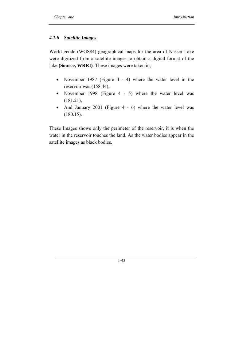
4.1.6 Satellite Images

World geode (WGS84) geographical maps for the area of Nasser Lake

were digitized from a satellite images to obtain a digital format of the

lake (Source, WRRI). These images were taken in;

November 1987 (Figure 4 - 4) where the water level in the

reservoir was (158.44),

November 1998 (Figure 4 - 5) where the water level was

(181.21),

And January 2001 (Figure 4 - 6) where the water level was

(180.15).

These Images shows only the perimeter of the reservoir, it is when the

water in the reservoir touches the land. As the water bodies appear in the

satellite images as black bodies.


1-44

Figure 4 - 4: Boundaries of the lake obtained using a LANDSAT image

acquired November 1987


1-45


acquired November 1998


1-46


acquired January 2001


1-47

It can be noticed the change in shape of the reservoir from level to

another. In 1987 image when the water level is lower than the two other

images we can just see the Tushka spillway but in 1998 when the water

level is higher the spillway becomes submerged under the water and the

water can be seen in Tushka canal down stream the spillway.

4.2 Geo-Referencing the Data

The Geographic Information System (GIS) application has been

recognised as a powerful mean to integrate and analyse data from various

sources. It was used to project both the High Aswan Dam Reservoir maps

and the section points into the Universal Transverse Mercator grid Zone

36 (UTM36).

The cross section points along with the 3 contours of the reservoir

perimeter at levels (158.44), (181.21) and (180.15), obtained from the

satellite images, were used to form a group of scatter points (x,y,z) with

the (UTM36) as a defined projected coordinate system. These points will

be used later in the generation of the bathymetry mesh.

4.3 Mesh Generation

The Surface water Modeling System (SMS) interface was used during

this stage as it is a graphical aided interface of creating the mesh, and it

also can support the file format used by many of hydrodynamic modeling

programs.

After creating a polygon which encloses the study area a mesh was

generated using the adaptive tessellation technique which is a mesh

generation technique used to fill the interior of a polygon.


1-48

The technique uses the existing spacing on the polygons to determine the

element sizes on the interior. Any interior arcs and refine points are

forced into the new mesh. If the input polygon has varying node densities

along its perimeter, SMS attempts to create a smooth element size

transition between these areas of differing densities. By altering the size

bias, the user can indicate whether SMS should favor the creation of

large or small elements. Decreasing the bias will result in smaller

elements; increasing the bias will result in larger elements (in this study

the bias was set to a value of 1.0 as the mesh size was already very large

and a small elements will cause a long time in calculations).

In either case, the elements in the interior of the mesh will honor the arc

edges and the element sizes specified at nodes. The bias simply controls

the element sizes in the transition region.

The mesh size was determined based on the capability of the available

hardware as increasing the mesh density will cause the solution time to

increase.

The spacing between nodes was chosen to be at an average of 250

meters. This resulted in a mesh of about (92,590) nodes and (43,540)

elements. Better results could be obtained with advanced hardware

capability.

To maintain good mesh properties the following points should be

reviewed after the mesh generation;

•A well constructed mesh must first have good element

properties.

•The overall bathymetric contours should be smooth.

•Wetting and drying studies work best when the element edges to

lie on bathymetric contours.

•Ideally, any boundary break angle should not exceed 10 degrees.


1-49

•Neighboring elements should not differ in size by more then

50%.

•Use adequate resolution to model the features of the prototype

plan.

•Maintain a length to width ratio of less than one to ten.

•Restrict element shapes to avoid highly distorted triangles or

rectangles.

•Create elements with corner angles greater than 10 degrees.

•Bathymetric elevations should lie almost in a plane.

•Maintain longitudinal element edge depth changes of less than

20%.

It should be noticed that most of the produced meshes will violate one or

all of these properties, but not excessively. They still are goals to strive

for. So, after the mesh was generated it was then checked out against

those errors as the SMS interface provided an automatic representation of

the mesh quality. Yet, it has to be corrected manually.

The errors (around 200 errors) were found in the mesh geometry and

were corrected manually by modifying the mesh elements to solve the

error according to its type. Some times an element was to be split into

more than one, another time it was to be merged or even deleted.


1-50

4.4 Bathymetry Interpolation

After the mesh generation, the scatter points obtained from the GIS were

used to form a triangles irregular net (TIN) which will be used in the

interpolation of the bed levels.

One of the most commonly used techniques for interpolation of scatter

points is inverse distance weighted (IDW) interpolation. Inverse distance

weighted methods are based on the assumption that the interpolating

surface should be influenced most by the nearby points and less by the

more distant points.

The interpolating surface is a weighted average of the scatter points and

the weight assigned to each scatter point diminishes as the distance from

the interpolation point to the scatter point increases.

The simplest form of inverse distance weighted interpolation is

sometimes called "Shepard's method" (Shepard 1968). The equation used

is as follows:

F(x,y) = i

n

ii fw

1

4. 4

where n is the number of scatter points in the set, fi are the prescribed

function values at the scatter points (e.g. the data set values), and wi are

the weight functions assigned to each scatter point. The weight function

varies from a value of unity at the scatter point to a value approaching

zero as the distance from the scatter point increases, and they are

normalized so that the weights sum to unity.

The effect of the weight function is that the surface interpolates each

scatter point and is influenced most strongly between scatter points by


1-51

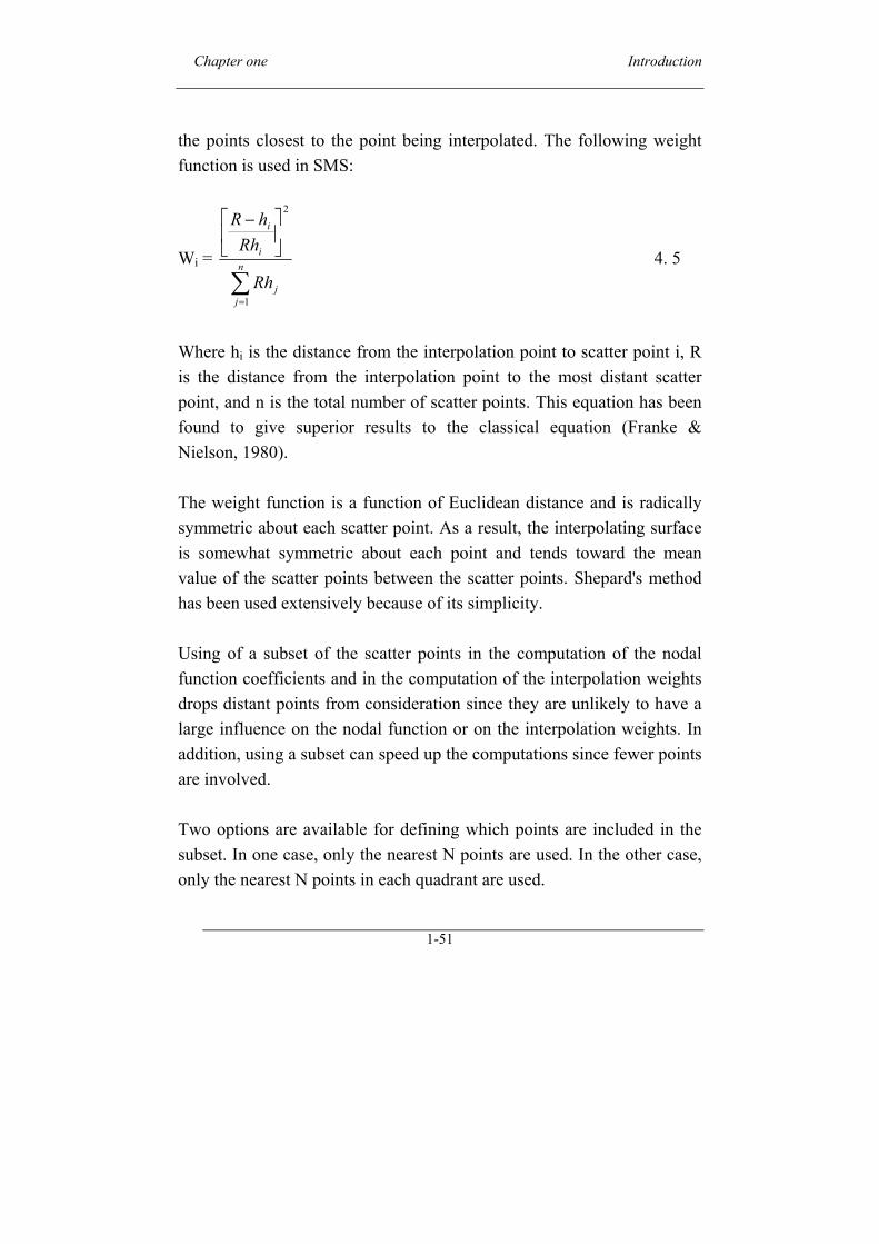
the points closest to the point being interpolated. The following weight

function is used in SMS:

Wi =

n

jj

i

i

Rh

Rh

hR

1

2

4. 5

Where hi is the distance from the interpolation point to scatter point i, R

is the distance from the interpolation point to the most distant scatter

point, and n is the total number of scatter points. This equation has been

found to give superior results to the classical equation (Franke &

Nielson, 1980).

The weight function is a function of Euclidean distance and is radically

symmetric about each scatter point. As a result, the interpolating surface

is somewhat symmetric about each point and tends toward the mean

value of the scatter points between the scatter points. Shepard's method

has been used extensively because of its simplicity.

Using of a subset of the scatter points in the computation of the nodal

function coefficients and in the computation of the interpolation weights

drops distant points from consideration since they are unlikely to have a

large influence on the nodal function or on the interpolation weights. In

addition, using a subset can speed up the computations since fewer points

are involved.

Two options are available for defining which points are included in the

subset. In one case, only the nearest N points are used. In the other case,

only the nearest N points in each quadrant are used.


1-52

If a subset of the scatter point set is being used for interpolation, a

scheme must be used to find the nearest N points. The scatter points are

triangulated to form a temporary TIN before the interpolation process

begins. To compute the nearest N points, the triangle containing the

interpolation point is found and the triangle topology is then used to

sweep out from the interpolation point in a systematic fashion until the N

nearest points is found. This scheme is fast for large scatter point sets.

Natural neighbor interpolation is also supported in SMS. It was first

introduced by Sibson (1981). A more detailed description of natural

neighbor interpolation in multiple dimensions can be found in Owen

(1992). The basic equation used in natural neighbor interpolation is

identical to the one used in IDW interpolation.

The difference between IDW interpolation and natural neighbor

interpolation is the method used to compute the weights and the method

used to select the subset of scatter points used for interpolation.

Natural neighbor interpolation is based on the Thiessen polygon network

of the scatter point set. The Thiessen polygon network can be constructed

from the Delauney triangulation of a scatter point set. A Delauney

triangulation is a TIN that has been constructed so that the Delauney

criterion has been satisfied.

There is one Thiessen polygon in the network for each scatter point. The

polygon encloses the area that is closer to the enclosed scatter point than

any other scatter point. The polygons in the interior of the scatter point

set are closed polygons and the polygons on the convex hull of the set are

open polygons.

Each Thiessen polygon is constructed using the circumcircles of the

triangles resulting from a Delauney triangulation of the scatter points.


1-53

The vertices of the Thiessen polygons correspond to the centroids of the

circum circles of the triangles.

To obtain good results from the interpolation of the bed, the Natural

neighbor technique was used for the interpolation and the inverse

distance technique for the extrapolation. 4.5 Enhancing the Resulted Bathymetry

After interpreting the first resulted bathymetric contours it was found that

this bathymetry should be enhanced because some parts were not covered

by the hydrographical survey may cause errors both in the Sudanese part

where the stream is narrower and in the Egyptian part.

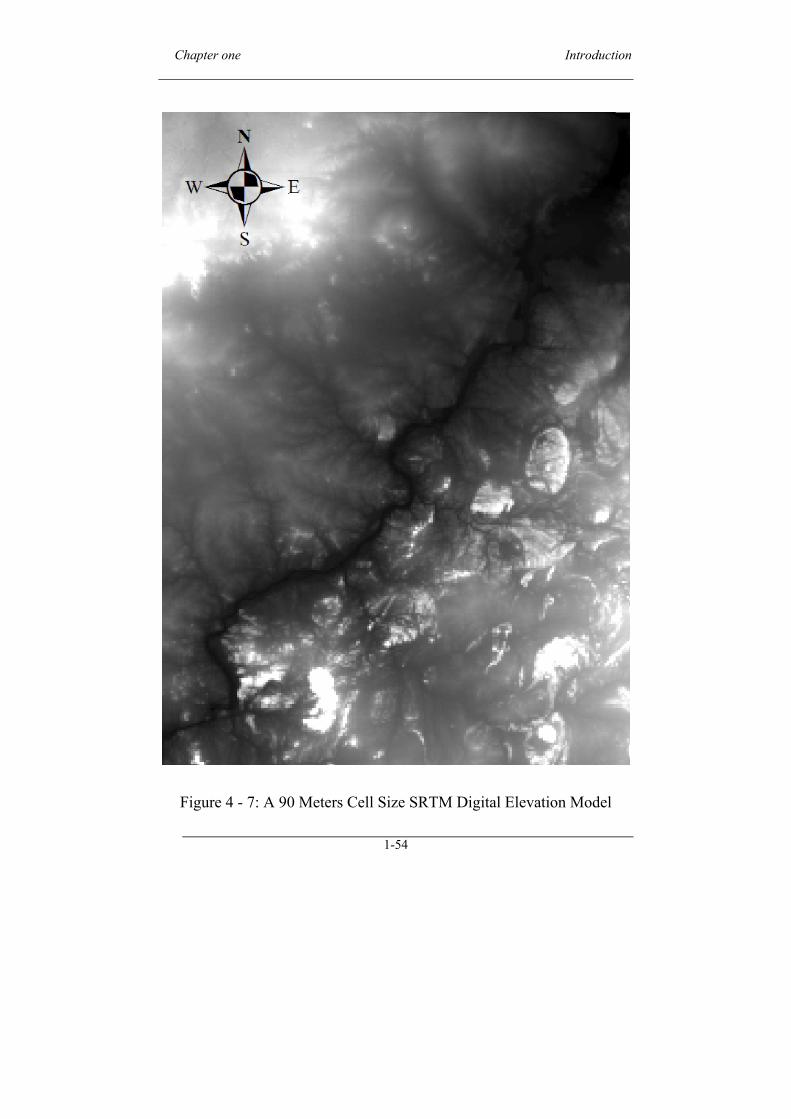
Therefore a Digital Elevation Model (DEM) of the surrounding area

(Figure 4-7) was used to generate a Triangulated Irregular Network

(TIN) using the GIS software. The DEM is a raster image divided into a

group of cells and each cell has a value the represent the elevation of its

location.

The resulted TIN (Figure 4 - 8) was then used in the interpolation process

to enhance the bathymetric contours. The Enhanced Bathymetry is shown

in Figure 4-9.


1-54

Figure 4 - 7: A 90 Meters Cell Size SRTM Digital Elevation Model


1-55

Figure 4 - 8: The Resulted TIN


1-56

Figure 4 - 9: The Resulted Bathymetry


1-57

4.1 Data Presentation ...................................................................................................... 35

4.1.1 Introduction: 35 4.1.2 The Inflow Data: 36 4.1.3 The Outflow Data: 38 4.1.4 The Cross Sections Geometric Data: 38 4.1.5 Longitudinal Section 41 4.1.6 Satellite Images 43

4.2 Geo-Referencing the Data ........................................................................................ 47 4.3 Mesh Generation ...................................................................................................... 47 4.4 Bathymetry Interpolation .......................................................................................... 50 4.5 Enhancing the Resulted Bathymetry ........................................................................ 53

Figure 4 - 1: Maximum Recorded hydrograph at Donqola station .......... 37 Figure 4 - 2: Cross section at Adenean in the year 2000 ......................... 40 Figure 4 - 3: Longitudinal Section of the HAD Reservoir (1964-2000) . 42 Figure 4 - 4: Boundaries of the lake obtained using a LANDSAT image

acquired November 1987 ................................................... 44 Figure 4 - 5: Boundaries of the lake obtained using a LANDSAT image

acquired November 1998 ................................................... 45 Figure 4 - 6: Boundaries of the lake obtained using a LANDSAT image

acquired January 2001 ........................................................ 46 Figure 4 - 7: A 90 Meters Cell Size SRTM Digital Elevation Model ..... 54 Figure 4 - 8: The Resulted TIN ................................................................ 55 Figure 4 - 9: The Resulted Bathymetry ................................................... 56

Table 4 - 1: Distances of cross sections upstream HAD ...................... 39


1-58

CHAPTER FIVE

The Hydrodynamic Model 5.1 Model selection

Reliable assessment and resolution of river hydraulics issues depend on

the engineer’s ability to understand and describe, in both written and

mathematical forms, the physical processes that govern a river system.

Three categories of methods for predicting river hydraulic conditions

were identified by Rouse (1959).

The first and oldest uses engineering experience acquired from previous

practice by an individual. The second utilizes laboratory scale models

(physical models) to replicate river hydraulic situations at a specific site

or for general types of structures. The third category is application of

analytical (mathematical) procedures and numerical modeling.

Recent use of physical and numerical modeling in combination, guided

by engineering experience, is termed "hybrid modeling" and has been

very successful.

To decide if a multidimensional study is needed, or a one-dimensional

approach is sufficient, a number of questions must be answered. Is there

a specific interest in the variation of some quantity in more than one of

the possible directions? If only one principal direction can be identified,

there is a good possibility that a one-dimensional study will suffice.

One dimensional analysis implies that the variation of relevant quantities

in directions perpendicular to the main axis is either assumed or

neglected, not computed. Common assumptions are the hydrostatic


1-59

pressure distribution, well-mixed fluid properties in the vertical, uniform

velocity distribution in a cross section, zero velocity components

transverse to the main axis, and so on.

It is possible that actual transverse variations will differ so greatly from

the assumed variation that streamwise values, determined from a one-

dimensional study, will be in significant error. If flow velocities in

floodplains are much less than that in the main channel, actual depths

everywhere will be greater than those computed on the basis of uniform

velocity distribution in the entire cross section. It is possible that the

transverse variations will be of greater importance than the streamwise

values. This is of particular importance when maximum values of water

surface elevation or current velocity are sought.

The choice of appropriate analytical methods to use during a river

hydraulics study is predicated on many factors including the objectives,

the level of detail being called for, the regime of flow expected, the

availability of necessary data, and the availability of time and resources

to properly address all essential issues.

A Survey was made on the 2D Hydrodynamic models. The selection and

the comparison between models were based on the following points:

1- The availability.

2- The ability to be applied to calculate water levels and flow

distribution in rivers and reservoirs.

3- Easiness to learn and use.

4- The Availability of the documentation of the model.

5- Very good visual representation of the inputs and outputs

which helps in the interpretation of the results.


1-60

The DYNHYD a Hydrodynamic Program is a simple link-node

hydrodynamic program capable of simulating variable tidal cycles, wind,

and unsteady flows. It produces an output file that supplies flows,

volumes, velocities, and depths (time averaged) for the WASP modeling

system.

The hydrodynamics model DYNHYD is an enhancement of the Potomac

Estuary hydrodynamic model which was a component of the Dynamic

Estuary Model. DYNHYD solves the one-dimensional equations of

continuity and momentum for a branching or channel-junction (link-

node), computational network. Driven by variable and downstream

heads, simulations typically proceed at one- to five-minute intervals. The

resulting unsteady hydrodynamics are averaged over larger time intervals

and stored for later use by the water quality program.

The hydrodynamic model solves one-dimensional equations describing

the propagation of a long wave through a shallow water system while

conserving both momentum (energy) and volume (mass). The equation

of motion, based on the conservation of momentum, predicts water

velocities and flows.

The equation of continuity, based on the conservation of volume, predicts

water heights (heads) and volumes. This approach assumes that flow is

predominantly one-dimensional, Coriolis and other accelerations normal

to the direction of flow are negligible, channels can be adequately

represented by a constant top width with a variable hydraulic depth, i.e.,

rectangular, the wave length is significantly greater than the depth, and

bottom slopes are moderate.

Although no strict criteria are available for the latter two assumptions,

most natural flow conditions in large rivers and estuaries would be


1-61

acceptable. Dam-break situations could not be simulated with DYNHYD

nor could small mountain streams.

TUFLOW (Two-dimensional Unsteady FLOW) is a two-dimensional

(2D) and one dimensional (1D) flood and tide simulation software. It

simulates the hydrodynamics of water bodies using 2D and 1D free-

surface flow equations. TUFLOW is specifically orientated towards

establishing flow patterns in coastal waters, estuaries, rivers and

floodplains where the flow patterns are essentially 2D in nature and

cannot or would be awkward to represent using a 1D network model.

A powerful feature of TUFLOW is its incorporation of the 1D

hydrodynamic network software, ESTRY (i.e. 2D and 1D domains are

linked to form one integrated model). TUFLOW continues to develop

and evolve to meet the challenges of hydrodynamic modeling. Its

strengths include rapid wetting and drying, powerful 1D and 2D linking

options, multiple 2D domains, 1D and 2D representation of hydraulic

structures, automatic flow regime switching over levees and

embankments, 1D and 2D supercritical flow, effective data handling and

quality control outputs. It is suited to modeling flooding in major rivers

through to complex overland and piped urban flows, and estuarine and

coastal hydraulics. TUFLOW uses GIS to manage, manipulate and

present data, and third-party software such as SMS to view and animate

results.

The TUFLOW software continues to develop and evolve to meet the

challenges of hydraulic modeling. Its strengths are rapid wetting and

drying, powerful 1D and 2D linking options, multiple 2D domains, 1D

and 2D modeling of hydraulic structures, treatment of levees and

embankments, effective data handling, 1D and 2D supercritical flow and

quality control outputs. TUFLOW is applicable for modeling flooding in

major rivers through to complex overland and piped urban flows, and


1-62

estuarine and coastal hydraulics. TUFLOW uses GIS as its primary

method of data management, manipulation and presentation. The use of

GIS allows easy inclusion of model topography changes to assess

floodplain impacts.

AquaDyn is a powerful and easy-to-use hydrodynamic simulation model

essential for water resources engineering studies, risk assessment, and

impact studies. AquaDyn allows the complete description and analysis of

hydrodynamic conditions (e.g., flow rates and water levels) of open

channels such as rivers, lakes, or estuaries. Engineers, specialists, and

decision-makers can use the specialized modules of the simulation

package to predict impacts on water flow conditions. For instance,

AquaDyn provides a reliable way to forecast the consequences of

different activities such as dredging or building dikes, bridges piers, and

embankments. AquaDyn can be used to model steady and unsteady flows

in supercritical as well as subcritical conditions and therefore permits the

user to take into account and study the effects of weirs, contractions, and

tidal waves.

The RMA2 model under the SMS interface was selected in the case

study and will be described in the following sections.

5.1.1 Origin of the Program

The original RMA2 was developed by Norton, King and Orlob (1973), of

Water Resources Engineers, for the Walla Walla District, Corps of

Engineers, and delivered in 1973. Further development, particularly of

the marsh porosity option, was carried out by King and Roig at the

University of California, Davis. Subsequent enhancements have been

made by King and Norton, of Resource Management Associates (RMA),

and by the Waterways Experiment Station (WES) Coastal and Hydraulics

Laboratory-USA, culminating in the current version of the code.


1-63

5.1.2 Model Description

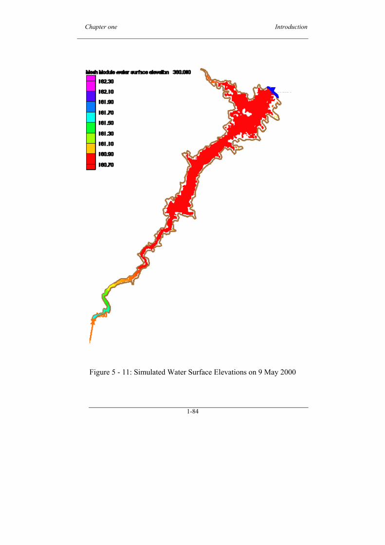
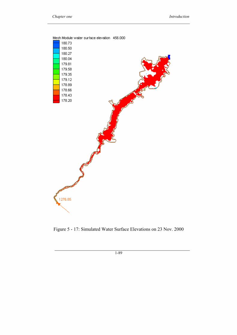
RMA2 is a two-dimensional depth averaged finite element hydrodynamic

numerical model. It computes water surface elevations and horizontal

velocity components for subcritical, free-surface two-dimensional flow

fields.

RMA2 computes a finite element solution of the Reynolds form of the

Navier-Stokes equations for turbulent flows. Friction is calculated with

the Manning’s or Chezy equation, and eddy viscosity coefficients are

used to define turbulence characteristics. Both steady and unsteady

(dynamic) problems can be analyzed.

The program has been applied to calculate water levels and flow

distribution around islands, flow at bridges having one or more relief

openings, in contracting and expanding reaches, into and out of off-

channel hydropower plants, at river junctions, and into and out of

pumping plant channels, circulation and transport in water bodies with

wetlands, and general water levels and flow patterns in rivers, reservoirs,

and estuaries.

5.1.3 Limitations of RMA2

RMA2 operates under the hydrostatic assumption; meaning accelerations

in the vertical direction are negligible. It is two-dimensional in the

horizontal plane. It is not intended to be used for near field problems

where vortices, vibrations, or vertical accelerations are of primary

interest. Vertically stratified flow effects are beyond the capabilities of

RMA2 and velocity vectors generally point in the same direction over the

entire depth of the water column at any instant of time. It expects a

vertically homogeneous fluid with a free surface.


1-64

RMA2 is a free-surface calculation model for subcritical flow

problems. More complex flows where vertical variations of variables are

important should be evaluated using a three-dimensional model, such as

RMA10.

The generalized computer program RMA2 solves the depth-integrated

equations of fluid mass and momentum conservation in two horizontal

directions by the finite element method using the Galerkin method of

weighted residuals.

0)( 22

3/1

2

2

2

2

2

vu

h

gun

x

h

x

agh

y

uE

x

uE

h

y

uhv

x

uhu

t

uh xyxx

0)( 22

3/1

2

2

2

2

2

vu

h

gvn

y

h

y

agh

y

vE

x

vE

h

y

vhv

x

vhu

t

vh yyyx

Where;

h = Depth

u, v = Velocities in the Cartesian directions

x, y, t = Cartesian coordinates and time

ρ = Density of fluid

E = Eddy viscosity coefficient,

for xx = normal direction on x axis surface

for yy = normal direction on y axis surface

for xy and yx = shear direction on each surface

g = Acceleration due to gravity

a = Elevation of bottom


1-65

n = Manning's roughness n-value The shape functions are quadratic for velocity and linear for depth.

Integration in space is performed by Gaussian integration. Derivatives in

time are replaced by a nonlinear finite difference approximation.

The solution is fully implicit and the set of simultaneous equations is

solved by Newton-Raphson non linear iteration. The computer code

executes the solution by means of a front-type solver, which assembles a

portion of the matrix and solves it before assembling the next portion of

the matrix.


1-66

5.2 The Modeling Process

The following flow chart illustrates the RMA2 modeling process.

Figure 5 - 1: Flow chart for the RMA2 modeling process

The Geometry File GENeration program (GFGEN) creates geometry and

finite element mesh files for input to the modeling system programs.

RMA2 Run Control file

Map Points

ASCII Geometry

GFGEN

Binary Geometry

Results Listing

Full Results Listing RMA2

Binary Solution


1-67

When RMA2 is used for a dynamic (unsteady state) simulation, it first

must solve a steady state problem. The results from this steady state case

are used to start the dynamic simulation. Unless specified otherwise,

RMA2 will continue directly from the steady state solution and begin the

dynamic simulation.

5.3 Guidelines for Obtaining a Good Solution

All aspects of the geometry and the numerical model simulation must run

in harmony. In addition to the geometry, the RMA2 run control

(boundary condition) file must contain the proper information if the

simulation is to be successful. A graphical user interface will help in

building a run control file, but it is a must to examine that file and double

check the run control selections.

The primary requirement for a successful numerical model is preparing a

good mesh; developing it with the following recommended guidelines in

mind. These guidelines are briefly described below.

Maintain Good Element Properties

● Maintain a length to width ratio of less than one to ten.

● Restrict element shapes to undistorted triangles or rectangles.

● Create elements with corner angles greater than 10 degrees.

● All bathymetric elevations should lie in one plane.

● Maintain longitudinal element edge depth changes of less than

20%.

Maintain Good Mesh Properties

● A well constructed mesh must first have good element

properties.

● The overall bathymetric contours should be smooth.


1-68

● Wetting and drying studies need the element edges to lie on

bathymetric contours.

● Ideally, any boundary break angle should not exceed 10

degrees.

● Neighboring elements should not differ in size by more then

50%.

● Use adequate resolution to model the features of the prototype

plan field.

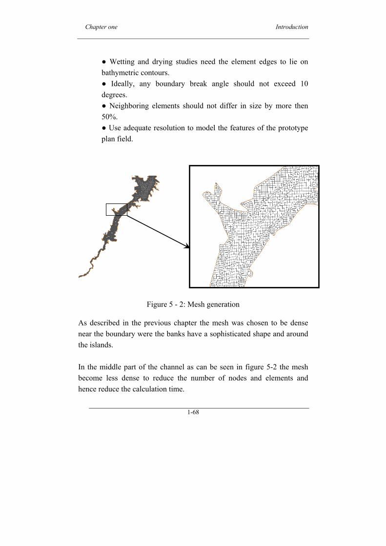
Figure 5 - 2: Mesh generation

As described in the previous chapter the mesh was chosen to be dense

near the boundary were the banks have a sophisticated shape and around

the islands.

In the middle part of the channel as can be seen in figure 5-2 the mesh

become less dense to reduce the number of nodes and elements and

hence reduce the calculation time.


1-69

5.4 Specifying Boundary Conditions

Boundary conditions usually take the form of a specified total discharge

at inflow sections and fixed water surface elevations or rating curves at

outflow sections. Since 2D models make no implicit assumptions about

flow direction or magnitude, discharge divisions in splitting channels and

the discharge given inflow and outflow elevations can be calculated

directly.

Locating flow boundaries some distance from areas of interest is

important to minimize the effect of boundary condition uncertainties.

Initial conditions are important, even for steady flow, since they are

usually used as the initial guess in the iterative solution procedure. A

good guess will significantly reduce the total run time and may make the

difference between a stable run and an unstable one.

Boundary conditions are required to drive RMA2 throughout a

simulation. They are constraints which are applied along the flow

boundaries of the solution domain, and required to eliminate the

constants of integration that arise when numerically integrating the

"Boundary conditions" is a mathematical term which specifies the

loading for a particular solution to a set of partial differential equations.

In more practical terms, boundary conditions for an unsteady flow model

are the combination of flow and stage time series, which when applied to

the exterior of the model either duplicates an observed event or generates

a hypothetical event such as a design flood. For an observed event, the

accuracy of the boundary conditions affects the quality of the

reproduction.

In a similar but less detectable manner the reasonableness of the

boundary conditions for a hypothetical event (because accuracy can

seldom be established) limits the quality of the conclusions. Furthermore,


1-70

the way that the boundary conditions are applied can control the overall

accuracy and consistency of the model.

External boundary nodes along the downstream end of the network are

typically assigned a water-level (head) boundary condition. Also,

boundary nodes along the upstream end of the network are typically

assigned an exact flow or discharge boundary condition.

Each side wall of the network is automatically assigned a parallel flow

boundary condition (i.e., slip flow) which allows the program to calculate

the velocity adjacent and parallel to the side wall as well as the flow

depth there.

Boundary conditions may be specified on a nodal basis, along the edge of

an element, or across a continuity check line. No special equations are

required for boundary nodes. The use of a boundary condition

specification removes either the depth, or one or both of the velocity

components from the computations, and the program expects those

values to be entered as boundary input data.

All boundary conditions hold from one time step to the next unless they

are specifically modified. RMA2 does not permit a new boundary

condition location to be specified in mid-run, nor does it allow a change

in the type of boundary condition at a previously specified boundary

location.


1-71

5.4.1 Upstream Boundary Condition

The recorded hydrographs at Donqola station 777 km upstream the HAD

forms the upstream boundary of the model and the maximum recorded

flood hydrograph (Figure 5-20) was used during the simulations.

5.4.2 Downstream Boundary Condition

The water level at the HAD was used as the downstream boundary

condition during the simulations. During the calibration and verification

processes the recorded water levels at the HAD station were used, Figure

5 - 3 shows the daily recorded levels from 1998 till 2002.


1-72

Figure 5 - 3: Water Level Recorded Upstream HAD (1996-2003)

170

172

174

176

178

180

182

01/01/1998

01/01/1999

01/01/2000

31/12/2000

31/12/2001

31/12/2002

31/12/2003

Date

Water Level (meter)


1-73

5.5 Model Checking For Continuity

Continuity refers to checking the water mass flux. The objective when

simulating is to retain the correct amount of fluid flow from one point to

the next, within a tolerance of about plus or minus 3%. Continuity check

lines provide a means to determine if your steady state simulation is

locally maintaining mass conservation at a given location.

Continuity check lines are typically used to estimate the flow rates at

cross-sections perpendicular to the flow path and serve as an error

indicator. The RMA2 model globally maintains mass conservation in a

weighted residual manner. Locally, continuity check lines can be used to

check for apparent mass changes in a different way, by direct integration.

Large discrepancies between the results of these two methods indicate

probable oscillations and a need to improve model resolution and/or to

correct large boundary break angles.

Although continuity checks are optional, they are a valuable tool for

diagnosing a converged steady state solution. For steady state, the

continuity check lines should represent total inflow equals total outflow.

However, if the continuity checks indicate a mass conservation

discrepancy of ±�3%, you may want to address the resolution in the

geometry.

5.6 Parameters Estimation

This pie chart (Figure 5 - 4) illustrates the approximate relative

importance to the simulation of the different aspects of an RMA2

simulation study. As it can be seen, the structure of the geometry and

overall study design are the most significant, followed by the boundary

condition assignments. The “other” category includes field data issues,


1-74

amount of time devoted to the effort, approach chosen to analyze data.

Study design includes model choice and boundary placement.

Geometry

BoundaryConditions

Roughness

Viscosity

Other

Figure 5 - 4: Relative Importance to Calibration

It may be fair enough to say that a model is only as good as its input data,

but it is true. As input data, 2D hydrodynamic models require channel

bed topography, roughness and transverse eddy viscosity distributions,

boundary conditions, and initial flow conditions. In addition, some kind

of discrete mesh or grid must be designed to capture the flow variations.

5.6.1 Bed Friction Computation

The bed friction energy transfer computation, or bottom roughness, is

one of the primary verification tools for RMA2. Changing the bed

friction provides some control over the fluid velocity magnitude and

direction.


1-75

Bed friction is typically calculated with Manning’s equation if the input

roughness value is < 3.0; otherwise a Chezy equation is used. By far, the

popular choice is Manning’s roughness coefficient (n) value, and these

roughness values may be assigned globally throughout the mesh by

material type, or on the elemental level.

RMA2 provides the means to input only the bottom roughness, not the

side wall roughness. Because there is no wall roughness in RMA2, it was

exaggerated on the elements forming the edge of the waterway in order

to approximate the wall roughness.

The roughness is a function of many variables such as type of bed and

bank materials, river geometry and irregularities. The accurate prediction

of the roughness in such case is a rather complicated task. The values of

Chezy and Manning’s roughness coefficient can be estimated using

references such as Chow (1959), Barnes (1967) and Krony (1992).

In this study, the Manning’s coefficient was taken as a constant value

over the river part and another constant value on the reservoir part to

make the simulation more easily those values were to be changed during

the simulation as when the water level rises the water covers more area

and the perimeter gets more irregular and this affects the roughness

values.

5.6.2 Specifying Turbulence

Turbulent exchanges are sensitive to changes in the direction of the

velocity vector. Conversely, small values of the turbulent exchange

coefficients allow the velocity vectors too much freedom to change

magnitude and direction in the iterative solution.


1-76

The result is a numerically unstable problem for which the program will

diverge rather than converge to a solution. One recourse is to continue

increasing the Eddy viscosity (E), until a stable solution is achieved.

There are many ways to control the turbulent exchange coefficient; (E)

one of them is the direct assignment method

The first and direct way to assign the turbulent exchange coefficient, E, is

to assign a particular value for each individual material type. As a

guideline for selecting reasonable values for the turbulent exchange

coefficients for a given material type the following algorithm were

followed:

1. A representative length of the elements within the material type

was determined (250 meter in average).

2. The dominant stream wise velocity for the given geometry

estimated ranged was in average of 0.05 m/s according to the

flow rate of about 2000 m3/s.

3. Then the Peclet number (P) equation was been solved for E

(Equation 5.1)

P = E

vdl 5.1

Where;

ρ�� = fluid density

v = average elemental velocity

dl = length of element in stream wise direction

E = Eddy Viscosity

Transverse eddy viscosity distributions are important for stability in some

finite difference and finite element models and are often assigned

unrealistically large values. They can be also be used as calibration

factors for measured flow distributions. Stable shock capturing and high


1-77

resolution numerical schemes are not sensitive to these values. In cases

where accurate determination of eddy viscosity is required, a coupled

turbulence model should be considered.

The Eddy viscosity used during the modeling process was found to be

equal to 1500 kg/m.s. and that gave an average value of Peclet No. equal

to 5.

5.7 Model Calibration

Some numerical modelers refer to calibration and verification as a two-

step process. Using this terminology, adjustments are made to model

coefficients and inputs so as to optimize agreement between model and

observed prototype data during the calibration step.

Then the model is run to attempt reproduction of a different set of

prototype data without further model adjustment. If the second run is

satisfactory then the model may be considered as verified.

This procedure sounds imminently reasonable, but experience suggests

that it is a naïve approach and it faces some problems such as:

1. All field data include errors, and sometimes dramatic errors.

Thus, they are not an absolute standard.

2. Field measurements include a variety of effects that may not be

reproduced in the model (for example, groundwater flow into

the model).

3. Conditions often change between field surveys, implying that

coefficients should also change (for example, differences in

bed forms at different flows may dictate a change in bed

roughness coefficients).


1-78

4. Most natural waterways cannot be adequately characterized by

two field data sets. Five or ten may be needed, but available

resources usually limit the field data.

5. If the model reproduces one field data set adequately, but not

the second, it should be decided whether to:

●Proceed with modeling, conceding an incomplete

verification.

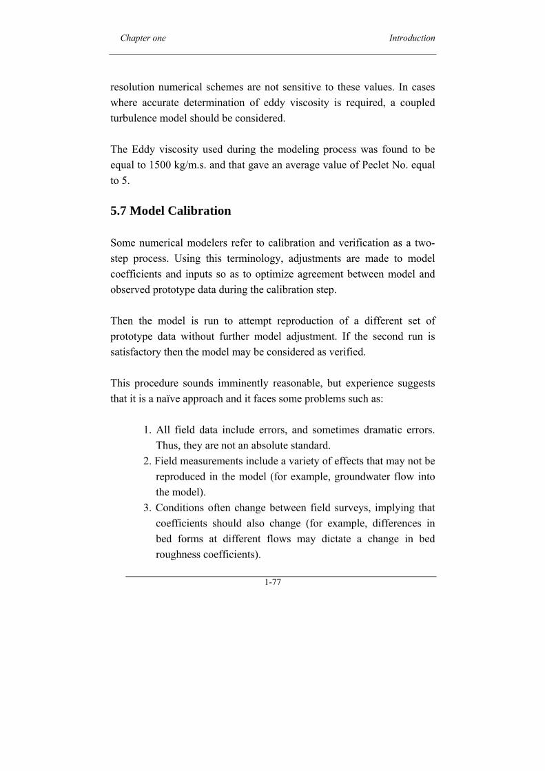
●Continue adjusting/revising to obtain a balanced quality of

reproduction.

●Conduct a re-analysis/re-collection of field data.

The objective of the calibration process is to match the output of the

model with observed data. This process is performed by adjusting one or

more parameters, such as Manning’s n, until a satisfactory match of

model results with known data is achieved.

When a set of known conditions has been approximately matched by the

model, one can apply the model to unknown conditions with more

confidence that the model output is reasonably representative of the

physical processes associated with that event. However, to be confident,

the observed data for calibration should be obtained from an event that is

near the scale of the events to be modeled.

When a model is calibrated, the parameters which control the model’s

performance, primarily Manning’s n and reach storage, are determined.

The key to a successful calibration is to identify the true values of the

parameters which control the system and not to use values that

compensate for shortcomings in the geometry and/or the boundary

conditions.


1-79

The High Aswan Dam Reservoir can be divided into two parts or

segments during the modeling process according to stream width, these

parts are the river with a width ranging from 950 meters to about 2000

meters and the reservoir with a width more than 2000 meters and up to

about 15000 meters.

The river parts starts from the reservoir inlet in the Sudanese side of the

lake and ends 360 kilometers upstream HAD where the reservoir part

starts. During the calibration process each part was assumed to have a

different roughness value as the flow behaves differently when passing

through each segment, Figure 5 - 5 shows those two parts.

Figure 5 - 5: River part and Reservoir part


1-80

In the beginning with low flow rate the calibrated roughness was found to be equal to 0.04 through out the whole reservoir but it increased to about 0.09 in the river part at flow rate of about 7500 m3/sec and remained unchanged in the reservoir part. It then increased again to about 0.13 at flow rate of about 10,000 m3/sec then again to 0.15 at the peak discharge.

Figure 5 - 6 shows the values of roughness used in the calibration

process, those values were calculated when the downstream boundary

(water level upstream HAD) was assumed 175 m.

0.020

0.040

0.060

0.080

0.100

0.120

0.140

0.160

0.180

0 2000 4000 6000 8000 10000 12000 14000

Flow rate (cms)

Man

nin

g's

rou

ghn

ess

Figure 5 - 6: Values of calibration roughness coefficient

The calibration process where carried out using the recorded water levels

at various sections upstream High Aswan Dam during the mission of the

year 2000 of the High Aswan Dam Authority in the Sudanese part of the

reservoir. The water levels recorded at those sections are presented in

Figure 5 - 7 along with the date they were recorded on.


1-81

Figure 5 - 7: The measured water levels used in calibration process

Figure 5 - 8 shows the recorded water levels upstream HAD during the

simulation period which begins by the 20th of April 2000 and ends at the

15th of May 2000, and Figure 5 - 9 shows the corresponding recorded

discharges at Donqola station during the same period.

The travel time was calculated assuming that the flood wave celerity is as

1.5 times as the flow velocity that has an average of 0.25 m/sec in the

Sudanese sector of the lake as observed by the HADA. The travel time

was calculated from the upstream Station (Donqola) to the entrance of

the study reach and was found to be 9 days. So the boundary interval was

chosen more than 9 days later than the first recorded level.

178.20

178.25

178.30

178.35

178.40

178.45

340350360370380390400410

Distance US HAD (km)

Wate

r L

evel (

m)

1-May-00

2-May-00

3-May-00

4-May-00

5-May-00

6-May-00

7-May-00

8-May-00

9-May-00

Date

Observed Levels date


1-82

Figure 5 - 8: Water level U.S. HAD

Figure 5 - 9: Discharge recorded at Donqola station

800

900

1000

1100

1200

1300

1400

20-A

pr-0

0

22-A

pr-0

0

24-A

pr-0

0

26-A

pr-0

0

28-A

pr-0

0

30-A

pr-0

0

2-M

ay-0

0

4-M

ay-0

0

6-M

ay-0

0

8-M

ay-0

0

10-M

ay-0

0

12-M

ay-0

0

14-M

ay-0

0

Date

Dis

char

ge r

ecor

ded

at

Don

gola

(m

3 /s)

178

178.1

178.2

178.3

178.4

178.5

178.6

178.7

20-A

pr-0

0

22-A

pr-0

0

24-A

pr-0

0

26-A

pr-0

0

28-A

pr-0

0

30-A

pr-0

0

2-M

ay-0

0

4-M

ay-0

0

6-M

ay-0

0

8-M

ay-0

0

10-M

ay-0

0

12-M

ay-0

0

14-M

ay-0

0

Date

Wat

er L

evel

U.S

. HA

D


1-83

The measured levels during the simulation interval were compared with

the levels calculated from the model and the results were plotted as

shown in Figure 5 - 10. The results show an absolute error value ranging

from 0.8 cm to 8.01 cm, which is a good result.

178.00

178.10

178.20

178.30

178.40

178.50

178.60

178.70

178.80

340350360370380390400410


Wa

ter

Le

ve

l (m

)

Observed Levels Calculated Levels

Figure 5 - 10: Observed Vs calculated water levels

The model results can be shown in the following figures, which present

the resulted water levels and velocity magnitudes at the end of the

simulated interval.

The difference between the observed and calculated water levels at km

365 is due to uncertainty of geometric data at this zone during data

filtering process.


1-84

Figure 5 - 11: Simulated Water Surface Elevations on 9 May 2000


1-85

Figure 5 - 12: Simulated Velocity Magnitudes on 9 May 2000


1-86

5.8 Model Parameters Verification

Verification is a multi-step process of model adjustments and

comparisons, leavened with careful consideration of both the model and

the data. It is not a simple two-step (calibration – verification)

procedure. The purpose of numerical modeling, as stated by W. A.

Thomas, a retired research hydraulic engineer from WES, is to “gain

insight, not answers”.

The verification process where carried out using the recorded water

levels at various sections upstream High Aswan Dam during the mission

of the year 2000 of the High Aswan Dam Authority in the Egyptian part

of the reservoir. The water levels recorded at those sections are presented

in Figure 5-13 along with the date they were recorded on.

180.60

180.60

180.61

180.61

180.62

180.62

180.63

180.63

180.64

250260270280290300310320330340


Wa

ter

Le

ve

l (m

)

17-Nov-00

18-Nov-00

19-Nov-00

20-Nov-00

21-Nov-00

22-Nov-00

23-Nov-00

24-Nov-00

Da

te

Observed Levels Date

Figure 5 - 13: The measured water levels used in verification process


1-87

Figure 5-14 shows the recorded water levels upstream HAD during the

simulation period which begins by the 10th of November 2000 and ends

at the 25th, and Figure 5-15 shows the corresponding recorded discharges

at Donqola station during the same period.

Figure 5 - 14: Water level U.S. HAD

Figure 5 - 15: Discharge recorded at Donqola station

180.56

180.57

180.58

180.59

180.6

180.61

180.62

180.63

180.64

10-N

ov-0

0

11-N

ov-0

0

12-N

ov-0

0

13-N

ov-0

0

14-N

ov-0

0

15-N

ov-0

0

16-N

ov-0

0

17-N

ov-0

0

18-N

ov-0

0

19-N

ov-0

0

20-N

ov-0

0

21-N

ov-0

0

22-N

ov-0

0

23-N

ov-0

0

24-N

ov-0

0

25-N

ov-0

0

Date

Wat

er L

evel U

.S. H

AD

1600

1800

2000

2200

2400

2600

2800

3000

3200

10-N

ov-0

0

11-N

ov-0

0

12-N

ov-0

0

13-N

ov-0

0

14-N

ov-0

0

15-N

ov-0

0

16-N

ov-0

0

17-N

ov-0

0

18-N

ov-0

0

19-N

ov-0

0

20-N

ov-0

0

21-N

ov-0

0

22-N

ov-0

0

23-N

ov-0

0

24-N

ov-0

0

25-N

ov-0

0

Date

Disch

arge

rec

orded

at D

ongo

la (m

3 /s)


1-88

Those measured levels where compared with the levels calculated from

the model and the results were plotted as shown in Figure 5-16. The

results show an absolute error value ranging from 0.02 cm to 1.28 cm

which is a good result.

Figure 5 - 16: Observed Vs calculated water levels

The model results can be shown in the following figures, which present

the resulted water levels and velocity magnitudes at the end of the

simulated interval.

180.50

180.52

180.54

180.56

180.58

180.60

180.62

180.64

180.66

180.68

180.70

250260270280290300310320330340


Wa

ter

Le

ve

l (m

)

Observed Levels Calculated Levels


1-89

Figure 5 - 17: Simulated Water Surface Elevations on 23 Nov. 2000


1-90

Figure 5 - 18: Simulated Velocity Magnitudes on 23 Nov. 2000


1-91

5.9 The Steady State Simulations

During the steady state simulations analysis the Manning's roughness

coefficient (n) needed to be calibrated as the inflow rate increased from

about 1250 m3/sec at the beginning of the flood to more than 12,500

m3/sec at its peak value which is a quite big range.

Steady state simulations for a flow rate of (1250, 2500, 5000, 7500 and

10,000 m3/sec) were carried out to study the hydraulic gradient variation

in the reservoir corresponding to various flood events, the water surface

profiles resulted from this study are shown in Figure 5-19 and the

difference of water level from the water level upstream the HAD is

shown in Figure 5-20.


1-92

Figure 5 - 19: The water surface profiles in HADR

181

182

183

184

185

186

187

200

250

300

350

400

450

Dis

tanc

e U

S H

AD

(km

)

W ater L evel (m)

Q =

125

0 m

3/s

Q =

250

0 m

3/s

Q =

500

0 m

3/s

Q =

750

0 m

3/s


1-93

Figure 5 - 20: The water level change in HADR

012345

200

250

300

350

400

450

Dis

tanc

e U

S H

AD

(km

)

W ater L evel change (m)

Q =

125

0 m

3/s

Q =

250

0 m

3/s

Q =

500

0 m

3/s

Q =

750

0 m

3/s


1-94

5.9.1 Interpretation of the Results

From the pervious figures it was concluded that the water level is almost

constant up to 250 km upstream the HAD due to the backwater effect of

the dam then it began to change slightly up to 340 km upstream the HAD

with hydraulic gradient of about 4.2 x 10-6 that causes a rise in the water

surface elevation of less than 0.15 m as shown in Figure 5 - 20.

Then due to the sophisticated shape of the lake and the irregularity of the

cross section along the rest of the lake, this part is known as Elshalalat

which means the small waterfalls, the water surface gradient increases to

an average of 2.5 x 10-5 and causes a rapid change in the water level with

a rise of about 4.3 meters corresponding to a flow rate of 7500 m3/sec in

an average distance of 100 kilometers as shown in Figure 5 - 20 .

The resulted figures assure the difficulty of taking measurements of the

cross sections geometry or the flow characteristics in this part of the

reservoir (upstream station 350) during high floods. So the High Aswan

Dam Authority (HADA) send the missions during the month of April and

November when the flow rate is about 2000 m3/sec so they can manage

to take measurements during low velocity currents.


1-95

5.1 Model selection ......................................................................................... 58

5.1.1 Origin of the Program 62 5.1.2 Model Description 63 5.1.3 Limitations of RMA2 63

5.2 The Modeling Process .............................................................................. 66 5.3 Guidelines for Obtaining a Good Solution ............................................ 67 5.4 Specifying Boundary Conditions ............................................................ 69

5.4.1 Upstream Boundary Condition 71 5.4.2 Downstream Boundary Condition 71

5.5 Model Checking For Continuity ............................................................. 73 5.6 Parameters Estimation .............................................................................. 73

5.6.1 Bed Friction Computation 74 5.6.2 Specifying Turbulence 75

5.7 Model Calibration ..................................................................................... 77 5.8 Model Parameters Verification ............................................................... 86 5.9 The Steady State Simulations .................................................................. 91

5.9.1 Interpretation of the Results 94

Figure 5 - 1: Flow chart for the RMA2 modeling process.................... 66 Figure 5 - 2: Mesh generation .......................................................... 68 Figure 5 - 3: Water Level Recorded Upstream HAD (1996-2003) ........ 72 Figure 5 - 4: Relative Importance to Calibration ................................ 74 Figure 5 - 5: River part and Reservoir part ........................................ 79 Figure 5 - 6: Values of calibration roughness coefficient ..................... 80 Figure 5 - 7: The measured water levels used in calibration process ..... 81 Figure 5 - 8: Water level U.S. HAD .................................................. 82 Figure 5 - 9: Discharge recorded at Donqola station ........................... 82 Figure 5 - 10: Observed Vs calculated water levels ............................ 83 Figure 5 - 11: Simulated Water Surface Elevations on 9 May 2000 ...... 84 Figure 5 - 12: Simulated Velocity Magnitudes on 9 May 2000 ............ 85 Figure 5 - 13: The measured water levels used in verification process .. 86 Figure 5 - 14: Water level U.S. HAD ................................................ 87 Figure 5 - 15: Discharge recorded at Donqola station ......................... 87 Figure 5 - 16: Observed Vs calculated water levels ............................ 88 Figure 5 - 17: Simulated Water Surface Elevations on 23 Nov. 2000 ... 89 Figure 5 - 18: Simulated Velocity Magnitudes on 23 Nov. 2000 .......... 90 Figure 5 - 19: The water surface profiles in HADR ............................ 92 Figure 5 - 20: The water level change in HADR ................................ 93


1-96


1-97

CHAPTER SIX

Unsteady State Simulation Time Step Control

Timing is introduced into the simulation when the boundary conditions

(head, velocity, discharge) vary in time. This is known as a dynamic or

unsteady state simulation. The time step used depends upon several

factors.

Although RMA2 uses an implicit solution scheme, some experimentation

is usually required when establishing the delta time step for dynamic

simulations. The modeling process started with a value appropriate for

the type of computations, and then the delta time step was increased to

the largest value that is numerically stable and physically representative

of the problem.

The time step is dependent on a dimensionless flow parameter called the

Courant number. Some hydrodynamic models developers suggest that to

maintain numerical stability and produce accurate results, the Courant

number should not exceed 1.0 (Westerink, Blain, Luettich, & Scheffner,

1994) while others (like the developers of MIKE21 in the DHI) say that it

should be kept under 5.0.The Courant number is defined as:

l

tghC N

6.1

Where:

g = acceleration due to gravity

h = nodal depth

Δt = time step (seconds)

Δl = nodal spacing


1-98

With each flow scenario, the increase (or decrease) in the flow rate will

affect the total volume of water in the system. Following the continuity

equation, higher flow rates will make the water surface elevation increase

due the larger volume of water in the river, causing numerical instability

if the same time step is used for all scenarios. Therefore, each flow

scenario uses a different Δt value.

In this case study the nodal depth varies along the reach an average of 5

meters depth in the river part to almost 60 meters in the reservoir part and

the average nodal spacing is equal to 250 meter and also varies in the

river part than the reservoir part.

One approach to select this interval in this case, is to employ a large time

step size and to run a test case in which the time step size is reduced until

the solution does not change, and use this interval as the time step size

during the simulation. Using such technique the step size during the

modeling process was taken equal to 12 hrs.

For dynamic simulation runs, the computational time interval should be

as small as necessary to capture the extremes of the dynamic boundary

conditions and maintain numerical stability. Yet, to reduce the

computational time taken to complete a simulation, the time step Interval

should be as large as possible, while small enough to still accurately

simulate the hydrodynamics of the modeled area.

The interval should be small enough to:

● Capture the extremes (highest and lowest peaks) of the

boundary condition signal. If the interval is too large, the peaks

of the signal may be missed.

● Accommodate rapid changes in water surface elevation.


1-99

Because unsteady flow models reproduce the entire range of flows, they

should be calibrated to reproduce both low and high flows.

A Factitious Flood Pulse Simulation

The first step taken was to simulate a factitious flood wave with a rapid

rising limb to study the wave propagation through the lake and test the

stability of the model with different unsteady flow rates.

The flood pulse shown in Figure 6 - 1 was used at the inlet and during

this simulation the water level at the downstream boundary was assumed

to be 180 m. The results of the 2D hydrodynamic model (Figures 6.1 to

6.6) showed the flood wave propagation in the reservoir, and the changes

to such wave in the downstream sections up till the High Aswan Dam.

From those resulted hydrographs it could be noticed that a hydrograph of

a 10,000 m3/s as a peak value and with a rising limb slope of 2000

m3/s/hr will travel trough the reservoir in about 16 hours and the peak

will fall to about 3500 m3/s which is, fortunately, dose not happen as the

real flood rising limb slope is much more milder than that. It could also

be noticed that most of the attenuation occurred in the reservoir part

when the width increases to more than 2500 m


1-100

Figure 6 - 1: An Input factitious Flood wave Pulse

0

2000

4000

6000

8000

1000

0

1200

0

01

23

45

67

89

1011

1213

1415

1617

1819

20

Tim

e (h

r)

discharge (m3

/s)


1-101

Figure 6 - 2: Hydrograph at section 5, 378 km upstream HAD

0

2000

4000

6000

8000

1000

0

1200

0

01

23

45

67

89

1011

1213

1415

1617

1819

20

Tim

e (h

r)

discharge (m3/s)


1-102


0

2000

4000

6000

8000

1000

0

1200

0

01

23

45

67

89

1011

1213

1415

1617

1819

20

Time (

hr)

discharge (m3/s)


1-103


0

2000

4000

6000

8000

1000

0

1200

0

01

23

45

67

89

1011

1213

1415

1617

1819

20

Tim

e (h

r)

discharge (m3/s)


1-104


0

2000

4000

6000

8000

1000

0

1200

0

01

23

45

67

89

1011

1213

1415

1617

1819

20

Tim

e (h

r)

discharge (m3/s)


1-105

Figure 6 - 6: Hydrograph at HAD

0

2000

4000

6000

8000

1000

0

1200

0

01

23

45

67

89

1011

1213

1415

1617

1819

20

Tim

e (h

r)

discharge (m3/s)


1-106

Study of Various Flood Waves

In order to study the flood wave propagation through the reservoir,

various simulations were carried out with different water levels in the

downstream of reservoir (182, 180, 178 and 175) meters and varying the

inflow rising and falling flood wave limbs slope (10, 20, 50) m3/s/hr.

First rising limb waves were applied to the model and the flood wave

movement was monitored through out the High Aswan Dam Reservoir

and the lag time, the outflow flood wave slope and the attenuation were

recorded.

These Results were summarized in the following figures.

4

6

8

10

12

0 10 20 30 40 50 60

Inflow Slope (m3/s/hr)

Lag

Tim

e (h

r)

175 178 180 182

Figure 6 - 7: Inflow rising flood wave slope Vs Lag time


1-107

0

500

1000

1500

2000

0 500 1000 1500 2000


Outflo

w S

lope

(m3 /s

/hr)

175 178 180 182

Figure 6 - 8: Inflow rising flood wave slope Vs Outflow flood wave slope

The interpretation of the previous curves yields to the derivation of these

relations,

Lt = 13.321(IS)-0.1457 6.2

With a least squared value = 0.8907

OS = 3.3496(IS)0.7365 6.3


Where,

Lt = Lag time in hours

IS = Inflow slope in m3/s/hr

OS = Outflow slope in m3/s/hr

Falling limb waves were applied to the model and the flood wave

movement was monitored through out the High Aswan Dam Reservoir


1-108

and the lag time and the outflow flood wave slope were recorded, these

Results were summarized in the following two figures.

0

5

10

15

20

25

0 10 20 30 40 50 60


La

g T

ime

(h

r)175 178 180 182

Figure 6 - 9: Inflow falling flood wave slope Vs Lag time


1-109

0

100

200

300

400

500

600

700

800

900

1000

0 500 1000 1500 2000


Ou

tflo

w S

lop

e (

m3 /s

/hr)

175 178 180 182

Figure 6 - 10: Inflow falling flood wave slope Vs Outflow wave slope

The interpretation of the previous two curves yields to the derivation of

these relations,

Lt = 22.99(IS)-0.1964 6.4


OS = 1.8132(IS)0.6793 6.5


Where,

Lt = Lag time in hours

IS = Inflow slope in m3/s/hr

OS = Outflow slope in m3/s/hr


1-110

It must be noticed that these charts and equations were developed

assuming that the downstream water level is kept to a pre-specified

values (175, 178, 180 and 182 m in our case) as a downstream boundary

condition.

There are three types of unsteady open channel waves commonly used in

civil engineering to study the behavior and progression of flood waves

(Ponce, 1989). The most complicated and generally applicable form of

flood wave is the dynamic wave, based on the St. Venant equations.

Kinematic waves are based solely on the principle of conservation of

mass within a control volume. This means that the difference between

inflow and outflow is equal to the change in storage volume, based on a

balance between friction and gravity.

Diffusion wave is more widely used because it applies to a wider range

of real flood waves. Most flood waves have some degree of physical

diffusion and this makes the applicability of this equation much wider.

From the resulted figures 6-7 and 6-9, it was concluded that the wave

travels through the reservoir in a kinematic nature that is the flood wave

speed is directly proportional with the depth of water.

If a downstream control structure such as the HAD exists at the

downstream this will cause the attenuation and the lag time to increase,

the following section will discuss the simulation of a real flood wave

with a control structure at the downstream end.


1-111

The Real Hydrograph Simulation

In this section a subroutine is developed to apply the real maximum

recorded hydrograph at Donqola station on the model with a controlled

downstream boundary condition and taking into consideration the

evaporation losses as estimated by the ministry of Irrigation (Figure 6 -

11).

0

2

4

6

8

10

12

Jan Feb Mar Apr May Jun Jul Aug Sep Oct Nov Dec

Month

Eva

pora

tion R

ate

(mm

/day

)

Figure 6 - 11: Estimates of Monthly Evaporation Rates From (HADR) Source: Omar, M.H. and El-Bakry (1970)

The hydraulic routing of the flood started at the beginning of August with

an initial water level in the reservoir of 175.00 meters above mean sea

level, as it is recommended by the ministry of irrigation to start the flood

year by the water level not more than this value.


1-112

Hydrodynamic Reservoir Operation Model

The developed 2D hydrodynamic model was to be used in dam

operation, to help predicting the water levels in the reservoir.

Unfortunately, this model can not simulate a controlled structure in the as

a downstream boundary condition.

Some modification had to be made to the model so it can be used in the

dam operation. The following section describes such procedure.

The storage in the reservoir was calculated from the model results using

the following equation:

ΔStorage = (Inflow – Demand – Tushka spillway overflow – Evaporation

Losses) ∆t

Figure 6 - 12 illustrate the storage volume in the reservoir versus the

water level (Egyptian Ministry of Irrigation, High Aswan Dam

Authority). From which a relation between the storage volume of the lake

and the water level could be derived (equation 6.6).


1-113

50

70

90

110

130

150

170

190

160 170 180 190Water Level (m)

Vo

lum

e (

bill

ion

m3 )

Figure 6 - 12: Storage Vs Water Level in the Reservoir

S = 2 x 10-15 x (WL)7.4647 6.6

Where:

S is the stored water volume in billion cubic meters.

WL is the water level in the reservoir.

Tushka spillway overflow can be calculated from the water level using

the following equation (M.Abdel Motaled and A.Allaithy) Hydraulic

Research Institute (HRI) 1998:

QTushka = 2.012 B (WL – Crest Level)1.569 6.7

Where:

B is the spillway crest width in meters.


It should be noticed from the equation that the spillway starting to release

water when the water level is above its crest level.


1-114

Figure 6 - 13 illustrate the reservoir surface area versus the water level

(Egyptian Ministry of Irrigation, High Aswan Dam Authority). From

which a relation between the surface area of the lake and the water level

could be derived (equation 6.8). The evaporation losses were then

calculated in m3/s by multiplying the surface area by the evaporation rate

Figure 6 - 11.

3000

4000

5000

6000

7000

8000

160 165 170 175 180 185 190

Water Level (m)

Are

a (

km

)2

Figure 6 - 13: Surface area Vs Water Level in the Reservoir

A = 1 x 10-10 x (WL)6.0889 6.8

Where:

A is surface area in square kilometers.



1-115

The Model Modification Process

The Hydrodynamic model was modified to be used in the routing process

of the real flood by following this algorithm:

1. The routing starts by the 1st of August with the water level in the

reservoir equals to (175.00) meter above the mean sea level.

2. A 10 days simulation interval was then carried out assuming the

downstream boundary condition equal to (175.00) meters.

3. The arrived flow at HAD was obtained, after running the

hydrodynamic model, and then compared with the water releases.

4. A Subroutine uses the Hydrodynamic model to evaluate the

downstream water surface boundary condition as will be

described in the following steps.

5. The difference between the arrived flow and the releases in this

interval was used to calculate the change in the storage using

equation (6.9) and (6.10):

ΔStorage = Δt x Σ(QArrived – QDemand) – ΔQEvaporation 6.9

ΔQEvaporation = Evaporation Rate x Surface Area 6.10

6. The new water volume in the reservoir was used to calculate the

new water level to be used as the downstream boundary condition

for the next 10 days interval using equation (6.6).

7. Another routing, 10 days interval, is to be started with the water

level calculated from step 6.


1-116

8. If the water level exceeded 178 meters the Tushka spillway will

begin to release flow and equation (6.11) should be modified.

ΔStorage =

Δt x Σ(QArrived – (QDemand + QTushka)) – ΔQEvaporation 6.11

Figure 6 - 14 shows the flow chart of the modification made to the

RMA2 model to simulate the real case study and the results of this

simulation are shown in Figure 6 - 15.


1-117

Figure 6 - 14: Flow chart of the modification made to RMA2

Flow at the downstream end. Water level at Tushka spillway.

Downstream water level

Subroutine constraints: Water level – Storage relation. Water level – Surface area relation.

Subroutine inputs: Water demands. Evaporation rates.

Subroutine to solve for D.S.water level using mass balance equation for HADR

RMA2

Hot start file to be used on each new time interval.

Output

Output Input

Input


1-118

The Modified Model Results

Figure 6 - 15: Inflow, Demand withdrawals, Tushka spillway outflow

and Evaporation losses Vs. Time

0

2000

4000

6000

8000

10000

12000

14000

01-

Aug

01-

Sep

02-

Oct

02-

Nov

03-

Dec

03-

Jan

03-

Feb

06-

Mar

06-

Apr

07-

May

07-

Jun

08-

Jul

Tim

e

Discharge (m3/sec)

Inflo

w

Dem

and

Toshka

Dem

and+

Toshka+

Eva

pora

tion

Eva

pora

tion


1-119

The resulted storage and water level upstream the HAD during 1 year

simulation period are shown in Figure 6 - 16.

Figure 6 - 16: Storage and Water level U.S. HAD Vs. Time

100

110

120

130

140

150

160 01

-Aug

01-S

ep02

-Oct

02-N

ov03

-Dec

03-J

an03

-Feb

06-M

ar06

-Apr

07-M

ay07

-Jun

08-J

ul

Tim

e

Storage (billion m3)

174

175

176

177

178

179

180

181

182

Water Level U.S. HAD (m)

Sto

rage

Wat

er L

evel


1-120

Interpretation of the Results

The decision makers put a scenario to insure that the water level by the

first of August is not more than (175.00) m. By applying this scenario the

maximum water level that would reached is (181.55) m by the mid of

October which is less than the maximum designed level.

It is proposed to start by the first of July with a water level in the

reservoir equal to (174.85) m when applying this scenario the water level

just reached the (182.00) m level by the mid of October, and that causes

increase of the storage in the reservoir by 2.898 billion cubic meters than

the currently proposed scenario.

The configuration of Tushka channel has to be modified to be able to

convey a maximum expected flow of about 5071 m3/s or the water level

may rise more than the calculated value as the downstream end of the

Tushka channel will control the flow diverted to the depression.


1-121

6.1 Time Step Control ............................................................................. 97 6.2 A Factitious Flood Pulse Simulation ................................................ 99 6.3 Study of Various Flood Waves ....................................................... 106 6.4 The Real Hydrograph Simulation ................................................... 111 6.5 Hydrodynamic Reservoir Operation Model .................................... 112

6.5.1 The Model Modification Process 115 6.5.2 The Modified Model Results 118 6.5.3 Interpretation of the Results 120

Figure 6 - 1: An Input factitious Flood wave Pulse ............................... 100 Figure 6 - 2: Hydrograph at section 5, 378 km upstream HAD ............ 101 Figure 6 - 3: Hydrograph at section 8, 357 km upstream HAD ............ 102 Figure 6 - 4: Hydrograph at section 10, 221 km upstream HAD .......... 103 Figure 6 - 5: Hydrograph at section 11, 135 km upstream HAD .......... 104 Figure 6 - 6: Hydrograph at HAD .......................................................... 105 Figure 6 - 7: Inflow rising flood wave slope Vs Lag time ..................... 106 Figure 6 - 8: Inflow rising flood wave slope Vs Outflow flood wave slope ............................................................................................................... 107 Figure 6 - 9: Inflow falling flood wave slope Vs Lag time ................... 108 Figure 6 - 10: Inflow falling flood wave slope Vs Outflow wave slope109 Figure 6 - 11: Estimates of Monthly Evaporation Rates From (HADR) ............................................................................................................... 111 Figure 6 - 12: Storage Vs Water Level in the Reservoir ....................... 113 Figure 6 - 13: Surface area Vs Water Level in the Reservoir................ 114 Figure 6 - 14: Flow chart of the modification made to RMA2 .............. 117 Figure 6 - 15: Inflow, Demand withdrawals, Tushka spillway outflow and Evaporation losses Vs. Time ........................................................... 118 Figure 6 - 16: Storage and Water level U.S. HAD Vs. Time ................ 119


1-122

CHAPTER SEVEN

High Aswan Dam Reservoir Simulator

General

The Previous chapters discussed the procedure followed to develop a two

dimensional hydrodynamic model for High Aswan Dam Reservoir. The

objective was to use such model for reservoir operation.

First the HAD reservoir bed surface was simulated then the

hydrodynamic model was developed, calibrated and verified resulting in

simulating the flow fields, steady and unsteady, of the reservoir.

The developed model was then applied on a real flood wave to test its

ability to be used for reservoir operation. But, the effort and time

consumed during such a process proved that a hydrodynamic model for

HADR is not a good tool to be used for dam operation. Yet, it can be

used in sedimentation or water quality studies.

The following sections describe the development of a hydrological model

(HADR Simulator) for dam operation along with its results.

Model Development

The model was based on the mass balance equation of the reservoir,

which can be described as the summation of the inflow equal the

summation of the out flow and can be represented in the following form:

The change in storage =

(Inflow – Releases – Tushka spillway overflow – Evaporation losses) ∆t


1-123

As the results of the hydrodynamic model show, the water level in the

reservoir is almost constant from the HAD upstream to Tushka spill way

the release over the weir can be directly calculated from the water level

using the weir equation presented in chapter six, equation 6.7.

The evaporation losses, Tushka overflow and storage can be calculated as

a function in water level as described in chapter six, equations 6.6 to 6.8.

The model developed interface have options to run for predefined

releases or it may be used to maximize the water level or, and the

hydropower. The flowchart, Figure 7 - 1, describes the model parts.

HADR Simulator Interface

The HADR Simulator interface was designed using the Visual Basic

programming language. It was designed to be used interactively through

out message boxes that pop out according to the user clicks.

It is easy to use as the input and output files are written and read in text

format, which can be exported to any data processing program that can

display them in charts.

Figure 7 - 2 shows the HADR Simulator starting window as you initiate

the program.


1-124

Dai

ly L

evel

s

Dai

ly R

elea

ses

Eva

luat

e O

bjec

tive

Fun

ctio

nF

orec

astin

g M

odel

Inpu

tsIn

flow

at D

ongo

la S

tatio

nA

vera

ge E

vapo

ratio

n R

ates

Opt

imum

Rul

ing

Sce

nari

o

HA

DR

Sim

ulat

or

Sele

ct a

noth

erru

ling

sce

nari

o

Res

ervo

ir O

ptim

izer

Mod

ule

for

HA

D

Mod

el C

onst

rain

ts M

odul

e

Init

ial W

ater

Lev

el

Sto

rage

- W

ater

Lev

el R

elat

ion

Are

a -

Wat

er L

evel

Rel

atio

n

Min

imum

Dem

ands

(N

avig

atio

n, I

rrig

atio

n an

d W

ater

Qua

lity)

Max

imum

allo

wab

le R

elea

ses

(Sco

urin

g an

d D

egra

datio

n)

Tos

hka

Q-H

Rel

atio

n

Out

put

Figure 7 - 1: Flow chart of HADR Simulator Model


1-125

Figure 7 - 2: HADR Simulator main window


1-126

Model Constraints

The model constraints can be summarized in the following points;

Maximum releases from HAD was assumed to be 280 million

m3/day as the maximum capacity of the river cross sections

downstream to prevent scouring of the bed downstream the Nile

Barrages.

Minimum releases from HAD was assumed to be 60 million

m3/day for navigation, hydropower and water quality reasons.

The released volume should not exceed Egypt share of Nile

water, which is 55.5 billion m3/year, according to the Nile Basin

Countries Agreement.

The starting water level upstream HAD before the beginning of

the year, and the target ending water level obtained from a long

term forecasting model.

Water level – Area and Water level – Storage relations.

Tushka spillway boundary conditions, as Water level – Q

relation.

Figure 7 - 3 shows the window used to change the model constraints

interactively during the model run, the present values are those driven

from equations presented in the previous chapter.


1-127

Figure 7 - 3: HADR Simulator, constraints window


1-128

Model Results Hydrodynamic model Versus HADR Simulator

After the model was developed, a comparison between its results and

those of the hydrodynamic model had to be made. The following figure

shows that both results almost match. The HADR Simulator proved to

be an easy and fast tool to be used in the reservoir management.

Figure 7 - 4: HADR Simulator results Vs Hydrodynamic model results

174

176

178

180

182

184

01-Aug 09-Nov 17-Feb 28-May

Time

Wat

er L

evel

U.S

. H

AD

(m

)

HADR Simulator Hydrodynamic Model


1-129

Effect of Varying the HAD Releases

The management of the reservoir flood concerns the control of the HAD releases in such a way that maximize the objective function of the model such as the water level and, or the hydropower. To test this effect, the developed model was used to calculate the water level with a two release scenarios, maximum and minimum, previously proposed by the High Aswan Dam Authority (HADA) and assuming the maximum recorded hydrograph at Donqola gagging station as the inflow at the upstream.

Figure 7 - 5 shows the results of those two scenarios from which it could be noticed that the proposed release scenario affect the water level during the period from the beginning of November to the end of April. During this period the incoming flood is in its peak while the demand is in its lowest values, as shown in Figure 7 - 6.

174

175

176

177

178

179

180

181

182

183

1-Aug 9-Nov 17-Feb 27-MayDate

Wat

er L

evel

U.S

. HAD (m

)

Case of max. releases Case of min. releases

Figure 7 - 5: Water levels resulted during maximum and minimum

proposed release scenarios


1-130

0

500

1000

1500

2000

2500

3000

3500

1-Aug 9-Nov 17-Feb 27-May

Date

Dem

and

s (m

3/s

)

Min Releases Max Releases

Figure 7 - 6: Maximum and minimum demands scenarios, previously

proposed by the HADA (1990-2003). Effect of Varying the Initial Water Level

The water level in the reservoir by the 1st of August, which is defined in

the model as the initial water level, is the level to start the simulation

with.

Various simulations were carried out to test the affect of varying this

level with maximum releases to the Nile River downstream HAD and

during a flood year, maximum expected flood recorded at Donqula

station. The resulted water levels upstream HAD during those

simulations are presented in Figure 7-7.


1-131

Figure 7 - 7: Water level U.S. HAD during a flood year and with

minimum releases scenario

16

0

16

2

16

4

16

6

16

8

17

0

17

2

17

4

17

6

17

8

18

0

18

2

18

4 1-A

ug

9-N

ov

17

-Fe

b2

7-M

ay

Da

te


Wl =

16

0 m

Wl =

16

5 m

Wl =

17

0 m

Wl =

17

2 m

Wl =

17

5 m

Wl =

17

8 m


1-132

From this figure, it could be noticed that, in case of a flood year the

initial starting water level will not affect the ending water level. As the

lake keep filling and the change in water level due to change in storage

will become slightly noticeable because the top width of the reservoir

cross sections become very wide, any small change in water level will

cause great variation in the total storage of the reservoir.

Almost all the proposed scenarios did not exceeded the maximum

designed level of the HAD, which is 182 meter above mean sea level.

Except, if we started with an initial water level of 178 m.

The ending water level, almost in all cases, will reach some where

between level 176 and level 177 meter which will cause threats to the

dam if two successive extreme floods is expected in two successive

years.

Another set of simulations were carried out to test the affect of varying

the initial water level in the reservoir with minimum releases to the Nile

River downstream HAD and during a drought year. The resulted water

levels upstream HAD during those simulations are presented in Figure 7-

8.


1-133

Figure 7 - 8: Water level U.S. HAD during a drought year and with

minimum releases scenario

145

150

155

160

165

170

175

180 1-A

ug

20-S

ep

9-N

ov

29-D

ec

17-F

eb

7-A

pr

27-M

ay

16-J

ul

Da

te


Wl =

160 m

Wl =

165 m

Wl =

170 m

Wl =

172 m

Wl =

175 m

Wl =

178 m


1-134

From this figure, it could be noticed that, in case of a drought year the

initial starting water level will affect the ending water level noticeably.

As the HAD Reservoir is releasing minimum demands to the

downstream, the change in water level due to change in storage becomes

noticeable, any small change in the storage will cause great variation in

the water level upstream the dam.

If the proposed initial level in the reservoir is less than 170 meter this

will cause great threat on the strategic storage of the water and may

reduce the power generated from the turbines to a very law levels. If we

started with an initial water level of 160 m or less this may cause to

completely empty the live storage from the reservoirs and cause the

turbines to shut down.

If two successive draught years followed each other this will threat the

country economy as the water level in the reservoir will fall below the

dead storage water level unless a release operation rule is suggested in

such case to reduce the release flow to the downstream as much as

possible.

Long Term Forecasting Model

The previous studies and figures could be used to simulate the water

level variation in the reservoir. Yet, a long term forecasting model is very

essential to propose a scenario for operation of the dam, from which a

target ending water level will be defined according the long term

forecasting.


1-135

Model Optimization

The developed model was designed to be used in an optimization process

with an objective functions to maximize the water level in the reservoir

and, or maximize the power output.

The Tushka spillway constraint can be modified in the calculations to

change its configurations, rise and lower its crest level or increase and

decrease its width. This will help in the long-term simulations and to

reduce the losses of water to Tushka depression during the draught years

and to release more water to it if there is a threat on the HAD.

The model begins the solution with an assumed releases derived from the

pattern of the previous recorded releases from the dam with constraints of

the minimum release required for navigation and water quality purposes.

The resulted water levels are stored and then another releases scenario is

assumed and the resulted water levels is then used along with the

previous results in the model optimization process, as described in Figure

7 - 1.


1-136

7.1 General ............................................................................................. 122 7.2 Model Development ........................................................................ 122

7.2.1 HADR Simulator Interface 123 7.2.2 Model Constraints 126

7.3 Model Results .................................................................................. 128 7.3.1 Hydrodynamic Versus HADR Simulator 128 7.3.2 Effect of varying the HAD releases 129 7.3.3 Effect of varying the initial water level 130

7.4 Long Term Forecasting Model ........................................................ 134 7.5 Model Optimization ......................................................................... 135

Figure 7 - 1: Flow chart of HADR Simulator Model ............................ 124 Figure 7 - 2: HADR Simulator main window ....................................... 125 Figure 7 - 3: HADR Simulator, constraints window ............................. 127 Figure 7 - 4: HADR Simulator results Vs Hydrodynamic model results ............................................................................................................... 128 Figure 7 - 5: Water levels resulted during maximum and minimum proposed release scenarios ..................................................................... 129 Figure 7 - 6: Maximum and minimum demands scenarios, previously proposed by the HADA. ........................................................................ 130 Figure 7 - 7: Water level U.S. HAD during a flood year and with minimum releases scenario .................................................................... 131 Figure 7 - 8: Water level U.S. HAD during a drought year and with minimum releases .................................................................................. 133


1-137

CHAPTER EIGHT

Conclusions and Recommendations

General

The study was carried out in order to develop a hydrodynamic two-

dimensional model for the High Aswan Dam Reservoir. This model is to

be used in several tasks such as:

Dam operation.

Sediment transport studies

Water quality studies.

As the work proceeded, it was found that, using the hydrodynamic model

for dam operation is a time consuming process and a hydrological model

will be sufficient for this task.

Conclusions

Based on the research results the following conclusions were obtained:

1. A Geo-database for the reservoir was built containing geometric

data, evaporation data with spatial variation, recorded inflow

hydrographs, recorded water levels at various, sediment data, etc.

2. A three dimensional surface of the HADR bed was generated as it

is a very important step for the hydrodynamic modeling.


1-138

3. A two-dimensional hydrodynamic model was developed to

simulate the flow fields (steady and unsteady) of the HADR as

the first 2D hydrodynamic model for the lake.

4. The hydraulic gradient in the High Aswan Dam Reservoir was

simulated and it was found that it varies between 4x10-6 during

low flood events (about 1000 m3/s) and more than 2.5x10-5 during

high flood events (about 7500 m3/s).

5. Various flow rates during different water levels were applied to

the model to study the wave movement through out the HADR.

And it was found that the flood wave travels through the reservoir

in a kinematic nature and the flood wave speed is directly

proportional with the depth of water.

6. Modifications were made to the hydrodynamic model so it can be

used in reservoir operation.

7. The decision makers put an operation rule to insure that the water

level by the first of August will not exceed (175.00) m. By

applying this rule, the maximum water level that would be

reached is (181.55) m by the mid of October which is less than

the maximum designed level.

8. Another proposed operation rule is to start by the first of July

with a water level in the reservoir of (174.85) m. By applying this

rule to the model, the maximum water level that was just reached

was (182.00) m level by the mid of October.

This will increase the strategic storage in the reservoir by 2.898

billion cubic meters than the currently proposed operation rule.


1-139

9. A modification has to be made to Tushka channel to convey a

discharge of about 5071 m3/s during high water levels.

10. A hydrological model for dam operation, HADR Simulator, was

developed for the purpose of dam operation.

11. The initial water level in the reservoir before the start of the flood

is very important factor to be considered during the management

process, Also is the target ending water level.

12. During flood years there is almost no danger on the HAD except

if we started at the 1st of August by a level more than 176 m.

13. If two successive high floods is expected the release scenario is to

be modified to insure that the water level upstream the HAD will

not exceed 182m.

14. During drought years the release scenario is to be modified to

insure that the water level upstream the HAD will not drop in a

dramatic way that threat the strategic storage in the reservoir.

15. For the purpose of dam operation a hydrological model is

sufficient with a reliable long term forecasting model of the Nile

basin.


1-140

Recommendations For future studies,

1. The HAD reservoir Geo-database should be updated as this may

cause some changes in the constraints of any reservoir model.

2. Further work should be done to update the bathymetry map

obtained specially on the Sudanese side because of sedimentation

and scouring process.

3. The data used in the calibration and verification (the velocity

fields) should have a spatial representation on the reservoir map

to help in the calibration process more effectively.

4. A short term forecasting model is very important for the modeling

of the reservoir.

5. More accurate results will be obtained if there is a long term

forecasting model to feed the operation model with the initial and

target ending water levels.

6. The results of the hydrodynamic model could be used in the

sediment transport and water quality studies of the reservoir.

7. Equipment for measuring spatial evaporation rates are needed to

fully evaluate the evaporation over the reservoir surface.

8. More effort should be made for the study of the ground water lake

interaction.


1-141

9. An operation rule for the releases of the HADR to the

downstream during successive drought year should be studied.

10. Flow automatic gagging stations are required along the reservoir

as the current stations which record water levels and discharge

about 700 km apart, HAD station and Donqola Station.

If intermediate stations records are available, the reservoir could

be divided in the simulation process into sub reaches using those

records. This will help in;

Reduce the processing time.

Reduce the time and effort taken in the calibration

process.


1-142

8.1 General 137 8.2 Conclusions 137 8.3 Recommendations 140

Date post:	10-Jul-2018
Category:	Documents
Upload:	lynhu
View:	213 times
Download:	0 times

Flood Routing Through Lake Nasser Using 2-D Model M...1-1 AIN SHAMS UNIVERSITY FACULTY OF...

Documents