1 Flow: Architecture and Benchmarking for Reinforcement Learning in Traffic Control Cathy Wu * , Aboudy Kreidieh † , Kanaad Parvate * , Eugene Vinitsky ‡ , Alexandre M Bayen *†§ * UC Berkeley, Electrical Engineering and Computer Science † UC Berkeley, Department of Civil and Environmental Engineering ‡ UC Berkeley, Department of Mechanical Engineering § UC Berkeley, Institute for Transportation Studies Abstract—Flow is a new computational framework, built to support a key need triggered by the rapid growth of autonomy in ground traffic: controllers for autonomous vehicles in the presence of complex nonlinear dynamics in traffic. Leveraging recent advances in deep Reinforcement Learning (RL), Flow enables the use of RL methods such as policy gradient for traffic control and enables benchmarking the performance of classical (including hand-designed) controllers with learned policies (con- trol laws). Flow integrates traffic microsimulator SUMO with deep reinforcement learning library rllab and enables the easy design of traffic tasks, including different networks configurations and vehicle dynamics. We use Flow to develop reliable controllers for complex problems, such as controlling mixed-autonomy traffic (involving both autonomous and human-driven vehicles) in a ring road. For this, we first show that state-of-the-art hand-designed controllers excel when in-distribution, but fail to generalize; then, we show that even simple neural network policies can solve the stabilization task across density settings and generalize to out- of-distribution settings. Index Terms—Learning and Adaptive Systems; Deep Rein- forcement Learning; Traffic Microsimulation I. I NTRODUCTION Transportation accounts for 28% of energy consumption in the US. Workers spent on aggregate over three million driver- years commuting to their jobs [1], with significant impact on nation-wide congestion. Based on 2012 estimates, U.S. commuters experienced an average of 52 hours of delay per year, causing $121 billion of delay and fuel costs annually [2]. Depending on its use in traffic, automation has the potential to achieve many benefits or to exacerbate problems at the system level, with potential amelioration or worsening of various system metrics including greenhouse gas (GHG) emissions, vehicle miles traveled (VMT), total travel time (TTT). Estimates project that 2% of fuel consumption today is wasted due to congestion, a figure that rises to 4.2% in 2050 [3]. As such, the potential efficiency improvement provided by autonomous vehicles is two to four percent of total fuel consumption due to the alleviation of congestion alone. In recent breakthrough experiments, Stern et al. [4] demon- strated a reduction in fuel consumption over 40% by the insertion of an autonomous vehicle in ring traffic to dampen the famous ring instabilities displayed by Sugiyama et al. in his seminal 2008 experiment [5]. This very disruptive field Corresponding author: Cathy Wu ([email protected]) Email addresses: {aboudy, kanaad, evinitsky, bayen}@berkeley.edu operational test is one of the motivations for the present work: it demonstrates the power of automation and its potential impact on complex traffic phenomena such as stop-and-go waves [6]. The breakthrough results [4], [7] are part of a broader core set of robotics challenges concerning the deployment of multi-agent automation systems, such as fleets of self- driving cars [8], [9], coordinated traffic lights [10], [11], or other coordinated infrastructure. Robotics has already demonstrated tremendous potential in improving transporta- tion systems through autonomous vehicles research; highly related problems include localization [12], [13], [14], path planning [15], [16], collision avoidance [17], and perception [18] problems. Considerable progress has also been made in recent decades in vehicle automation, including anti-lock braking systems (ABS), adaptive cruise control, lane keeping, automated parking, etc. [19], [20], [21], [22], which also have great potential to improve energy efficiency and safety in traffic. Down the road, the emergence of automated districts, i.e. districts where all vehicles are automated and operate efficiently with collaborative path-planning, might push this paradigm to next generation mobility [23]. Fleets of au- tonomous vehicles have recently been explored in the context of shared-mobility systems, such as autonomous mobility-on- demand systems, which abstracts out the low-level vehicle dynamics and considers a queuing theoretic model. Low- level vehicle dynamics, however, are of crucial importance, as exhibited by [24] and because many traffic phenomena, which affect energy consumption, safety, and travel time are exhibited at the level of low-level dynamics [5], [25], [26], [27]. In some settings, model-based controllers enable analytical solutions, or tractable algorithmic solutions. However, often, due to the nonlinearity of the models, numerous guarantees are lost in the process of developing controllers (i.e. optimality, run-time, complexity, approximation ratio, etc.). For example, while the ring setting enables elegant controllers to work in practice, the extension of these results (both theoretical and experimental) to arbitrary settings (network topologies, number of lanes, heterogeneity of the fleet, etc.) is challenging. Deep reinforcement learning (RL), which is the main en- abler in our framework, is a powerful tool for control and has already had demonstrated success in complex but data-rich problem settings such as Atari games [28], 3D locomotion and manipulation [29], [30], [31], chess [32], among others. arXiv:1710.05465v1 [cs.AI] 16 Oct 2017
Transcript
1
Flow: Architecture and Benchmarking forReinforcement Learning in Traffic ControlCathy Wu∗, Aboudy Kreidieh†, Kanaad Parvate∗, Eugene Vinitsky‡, Alexandre M Bayen∗†§
∗UC Berkeley, Electrical Engineering and Computer Science†UC Berkeley, Department of Civil and Environmental Engineering
‡UC Berkeley, Department of Mechanical Engineering§UC Berkeley, Institute for Transportation Studies
Abstract—Flow is a new computational framework, built tosupport a key need triggered by the rapid growth of autonomyin ground traffic: controllers for autonomous vehicles in thepresence of complex nonlinear dynamics in traffic. Leveragingrecent advances in deep Reinforcement Learning (RL), Flowenables the use of RL methods such as policy gradient for trafficcontrol and enables benchmarking the performance of classical(including hand-designed) controllers with learned policies (con-trol laws). Flow integrates traffic microsimulator SUMO withdeep reinforcement learning library rllab and enables the easydesign of traffic tasks, including different networks configurationsand vehicle dynamics. We use Flow to develop reliable controllersfor complex problems, such as controlling mixed-autonomy traffic(involving both autonomous and human-driven vehicles) in a ringroad. For this, we first show that state-of-the-art hand-designedcontrollers excel when in-distribution, but fail to generalize; then,we show that even simple neural network policies can solve thestabilization task across density settings and generalize to out-of-distribution settings.
Index Terms—Learning and Adaptive Systems; Deep Rein-forcement Learning; Traffic Microsimulation
I. INTRODUCTION
Transportation accounts for 28% of energy consumption inthe US. Workers spent on aggregate over three million driver-years commuting to their jobs [1], with significant impacton nation-wide congestion. Based on 2012 estimates, U.S.commuters experienced an average of 52 hours of delay peryear, causing $121 billion of delay and fuel costs annually[2]. Depending on its use in traffic, automation has thepotential to achieve many benefits or to exacerbate problemsat the system level, with potential amelioration or worseningof various system metrics including greenhouse gas (GHG)emissions, vehicle miles traveled (VMT), total travel time(TTT). Estimates project that 2% of fuel consumption today iswasted due to congestion, a figure that rises to 4.2% in 2050[3]. As such, the potential efficiency improvement providedby autonomous vehicles is two to four percent of total fuelconsumption due to the alleviation of congestion alone.
In recent breakthrough experiments, Stern et al. [4] demon-strated a reduction in fuel consumption over 40% by theinsertion of an autonomous vehicle in ring traffic to dampenthe famous ring instabilities displayed by Sugiyama et al. inhis seminal 2008 experiment [5]. This very disruptive field
operational test is one of the motivations for the present work:it demonstrates the power of automation and its potentialimpact on complex traffic phenomena such as stop-and-gowaves [6].
The breakthrough results [4], [7] are part of a broadercore set of robotics challenges concerning the deploymentof multi-agent automation systems, such as fleets of self-driving cars [8], [9], coordinated traffic lights [10], [11],or other coordinated infrastructure. Robotics has alreadydemonstrated tremendous potential in improving transporta-tion systems through autonomous vehicles research; highlyrelated problems include localization [12], [13], [14], pathplanning [15], [16], collision avoidance [17], and perception[18] problems. Considerable progress has also been madein recent decades in vehicle automation, including anti-lockbraking systems (ABS), adaptive cruise control, lane keeping,automated parking, etc. [19], [20], [21], [22], which also havegreat potential to improve energy efficiency and safety intraffic. Down the road, the emergence of automated districts,i.e. districts where all vehicles are automated and operateefficiently with collaborative path-planning, might push thisparadigm to next generation mobility [23]. Fleets of au-tonomous vehicles have recently been explored in the contextof shared-mobility systems, such as autonomous mobility-on-demand systems, which abstracts out the low-level vehicledynamics and considers a queuing theoretic model. Low-level vehicle dynamics, however, are of crucial importance, asexhibited by [24] and because many traffic phenomena, whichaffect energy consumption, safety, and travel time are exhibitedat the level of low-level dynamics [5], [25], [26], [27]. In somesettings, model-based controllers enable analytical solutions,or tractable algorithmic solutions. However, often, due to thenonlinearity of the models, numerous guarantees are lost inthe process of developing controllers (i.e. optimality, run-time,complexity, approximation ratio, etc.). For example, while thering setting enables elegant controllers to work in practice, theextension of these results (both theoretical and experimental)to arbitrary settings (network topologies, number of lanes,heterogeneity of the fleet, etc.) is challenging.
Deep reinforcement learning (RL), which is the main en-abler in our framework, is a powerful tool for control and hasalready had demonstrated success in complex but data-richproblem settings such as Atari games [28], 3D locomotionand manipulation [29], [30], [31], chess [32], among others.
arX
iv:1
710.
0546
5v1
[cs
.AI]
16
Oct
201
7
2
RL testbeds exist for different problem domains, such as theArcade Learning Environment (ALE) for Atari games [33],DeepMind Lab for a first-person 3D game [34], OpenAI gymfor a variety of control problems [35], FAIR TorchCraft forStarcraft: Brood War [36], MuJoCo for multi-joint dynamicswith Contact [37], TORCS for a car racing game [38], amongothers. DeepMind and Blizzard will collaborate to releasethe Starcraft II AI research environment [39]. Each of theseRL testbeds enables the study of control through RL of aspecific problem domain by leveraging of the data-rich settingof simulation. One of the primary goals of this article is topresent a similarly suitable RL testbed for traffic dynamics bymaking use of an existing traffic simulator.
These recent advances in deep RL provide a promisingalternative to model-based controller design, which the presentarticle explores. One key step in the development of suchparadigms is the ability to provide high fidelity microsimula-tions of traffic that can encompass accurate vehicle dynamicsto simulate the action of these new RL-generated controlpolicies, a pre-requisite to field experimental tests. This isprecisely one of the aims of the present article. RL promisesan approach to design controllers using black box machinelearning systems. It still requires physical vehicle responseto be incorporated in the simulation to learn controllers thatmatch physical vehicle dynamics. This problem extends be-yond the vehicle for which the controller is to be designed.For example, although vehicle velocity is intuitive as a controlvariable, it is important to keep in mind that other variables,such as actuator torques, are those actually controlled; anotherexample is that the input may consist of data from cameras,LIDAR, or radar. The conversion between the variables mightor might not be direct and may require the design of additionalcontrollers, the performance of which would also have to beconsidered.
In the present article, we propose the first (to our knowl-edge) computational framework and architecture to systemati-cally integrate deep RL and traffic microsimulation, therebyenabling the systematic study of autonomous vehicles incomplex traffic settings, including mixed-autonomy and fully-autonomous settings. Our framework permits both RL andclassical control techniques to be applied to microsimulations.As classical control is a primary approach for studying trafficdynamics, supporting benchmarking with such methods iscrucial for measuring progress of learned controllers. As anillustration, this article provides a benchmark of the rela-tive performance of learned and explicit controllers [4] forthe mixed-autonomy ring road setting. The computationalframework encompasses model-free reinforcement learningapproaches, which complement model-based methods such asmodel-based reinforcement learning, dynamic programming,optimal control, and hand-designed controllers; these methodsdramatically range in complexity, sometimes exhibiting pro-hibitive computational costs. Our initial case study investigatesmicroscopic longitudinal dynamics (forwards-backwards) [40]and lateral dynamics (left-right) [41] of vehicles. We studya variety of network configurations, and our proposed frame-work largely extends to other reinforcement learning methodsand other dynamics and settings, such as coordinated behaviors
[42], other sophisticated behavior models, and more complexnetwork configurations.
The contribution of this article includes three components,(1) a computational framework and architecture, which pro-vides a rich design space for traffic control problems andexposes model-free RL methods, (2) the implementation ofseveral instantiations of RL algorithms that can solve complexcontrol tasks, and (3) a set of use cases that illustratesthe power of the building block and benchmark scenarios.Specifically, our contributions are:
• Flow, a computational framework for deep RL and controlexperiments for traffic microsimulation. Flow integratesthe traffic microsimulator SUMO [43] with a standarddeep reinforcement learning library rllab [44], therebypermitting the training of large-scale reinforcement learn-ing experiments at scale on Amazon Web Services (AWS)Elastic Compute Cloud (EC2) for traffic control tasks.Our computational framework is open-source and avail-able at https://github.com/cathywu/flow.
• An interface, provided by Flow for the design of trafficcontrol tasks, including customized configurations of dif-ferent road networks, vehicle types and vehicle dynamics,noise models, as well as other attributes provided by astandard Markov Decision Process (MDP) interface.
• Extensions of SUMO to support high frequency simula-tion and greater flexibility in controllers.
• Exposing model-free reinforcement algorithms for dis-counted finite (partially observed) MDPs such as policygradient, with specific examples including Trust RegionPolicy Optimization (TRPO) [30] and Generalized Ad-vantage Estimation (GAE) [29], to the domain of trafficcontrol problems.
• Benchmarking of relative performance of learned andexplicit controllers in rich traffic control settings. Wepresent a benchmark on the mixed-autonomy single-lanering road network and find that a reinforcement learningagent is capable of learning policies exceeding the perfor-mance of state-of-the-art controllers. The particular caseof Sugiyama instabilities [5] is used to demonstrate thepower of our tool.
• Case studies for building block networks. We demon-strate deep RL results on traffic at the level of multi-agent vehicle control. We demonstrate all-human, mixed-autonomy, and fully-autonomous experiments on morecomplex traffic control tasks, such as a multi-lane ringroad and a figure 8 network. We provide additionalnetworks, including a merge network and an intersectionnetworks.
The rest of the article is organized as follows. Section IIprovides background on the RL framework used in the restof the article. Section III describes the architecture of Flowand the processes it can handle in the three computationalenvironments they are run (incl. SUMO and rllab). Sec-tion IV presents the various building blocks used by SUMOfor building general networks (underlying maps). Section Vpresents the various settings for the optimization, incl. action/ observation space, reward functions and policies. This is
3
followed by two experimental sections: in Section VI, in whichwe benchmark the performance of the RL-based algorithm tothe seminal FollowerStopper controller [4], and Section VIIwhich presents a series of various other experiments on thebuilding block network modules of Flow. Finally, Section VIIIpresents related work to place this in the broader context oftraffic flow modeling, deep RL and microsimulations.
II. PRELIMINARIES
In this section, we define the notation used in subsequentsections.
The system described in this article solves tasks whichconform to the standard interface of a finite-horizon discountedMarkov decision process (MDP) [45], [46], defined by thetuple (S,A, P, r, ρ0, γ, T ), where S is a (possibly infinite) setof states, A is a set of actions, P : S × A × S → R≥0
is the transition probability distribution, r : S × A → Ris the reward function, ρ0 : S → R≥0 is the initial statedistribution, γ ∈ (0, 1] is the discount factor, and T is thehorizon. For partially observable tasks, which conform to theinterface of a partially observable Markov decision process(POMDP), two more components are required, namely Ω, aset of observations, and O : S × Ω → R≥0, the observationprobability distribution.
RL studies the problem of how agents can learn to takeactions in its environment to maximize its cumulative reward.The Flow framework uses policy gradient methods [47], aclass of reinforcement learning algorithms which optimizea stochastic policy πθ : S × A → R≥0. These algorithmsiteratively update the parameters of the policy through opti-mizing the expected cumulative reward using sampled datafrom SUMO. The policy usually consists of neural networks,and may be of several forms. Two policies used in this articleare the Multilayer Perceptron (MLP) and Gated Recurrent Unit(GRU). MLP is a classical artificial neural network with mul-tiple hidden layers and utilizes backpropagation to optimize itsparameters [48]. GRUs are recurrent neural network capableof storing memory on the previous states of the system throughthe use of parametrized update and reset gates, which are alsooptimized by the policy gradient method [49]. This enablesGRUs to make decisions based on both current input and pastinputs.
The autonomous vehicles in our system execute controllerswhich are parameterized policies, trained using policy gradientmethods. For all experiments in this article, we use theTrust Region Policy Optimization (TRPO) [30] policy gradientmethod for learning the policy, linear feature baselines asdescribed in [44], discount factor γ = 0.999, and step size0.01. For most experiments, a diagonal Gaussian MLP policyis used with hidden layers (100, 50, 25) and tanh non-linearity. The experiment stabilizing the ring, described later,uses a hidden layer of shape (3,3). For experiments requiringmemory, a GRU policy with hidden layers (5,) and tanh non-linearity is used.
III. OVERVIEW OF FLOW
Flow is created to fill the gap between modern machinelearning and complex control problems in traffic. Flow is
Fig. 1: Flow Process Diagram. Flow interfaces SUMO via TraCI with rllab topermit the construction and simulation of traffic MDPs and for the training andevaluation of policies (control laws). After initializing the simulation in someinitial configuration, rllab collects samples by advancing and observing thesimulation. In each step, vehicles are provided actions through a pre-specifiedcontroller or through a policy (via rllab). These actions are then applied viaTraCI and the simulation progresses. At the end of an episode, rllab issuesa reset command to the environment, which returns vehicles to their initial(possibly random) position.
a computational framework for traffic microsimulation withRL methods. Although the architecture is agnostic to specificmachine learning and traffic software packages, we chose tointegrate widely used open-source tools to promote access andextension.
The first of those open-source tools is SUMO (Simulationof Urban MObility) [43]. SUMO is a continuous-time andcontinuous-space microscopic traffic simulator. It is capable ofhandling large road networks and of modeling the dynamics ofeach vehicle in the simulation. SUMO was chosen particularlyfor its extensibility, as it includes an API called TraCI (TrafficControl Interface). TraCI allows users to extend existingSUMO functionality through querying and modifying the stateof the simulation, at the single time-step resolution. Thisallows the user to easily provide intricate, custom commandsthat modify the simulation directly.
Secondly, we use rllab, an open source framework thatenables running and evaluating RL algorithms on a varietyof different scenarios, from classic tasks such as cartpolebalancing to more complicated tasks such as 3D humanoidlocomotion [44]. Flow uses rllab to facilitate the training, op-timization, and application of control policies that manipulatethe simulation. By modeling traffic scenarios as reinforce-ment learning problems, we use rllab to issue longitudinaland lateral controls to vehicles. Rllab further interfaces withOpenAI Gym, another framework for the development and
4
evaluation of reinforcement learning algorithms. The SUMOenvironments built in Flow are also compatible with OpenAIGym.
Flow encapsulates SUMO via TraCI to permit the defini-tion and simulation of traffic MDPs for rllab to train andevaluate policies. After initializing the simulation in someinitial configuration, rllab collects samples by advancing andobserving the simulation. In each step, vehicles are providedactions through a pre-specified controller or through a policy.These actions are then applied via TraCI and the simulationprogresses. After a specified number of timesteps (i.e. theend of a rollout) or after the simulation has terminated early(i.e. a vehicle has crashed), rllab issues a reset commandto the environment, which returns vehicles to their initial(possibly random) position. The interactions between Flow,SUMO/TraCI, and rllab are illustrated in Figure 1.
In addition to learned policies, Flow supports classicalcontrol (including hand-designed controllers and calibratedmodels of human dynamics) for longitudinal and lateral con-trol. Flow also supports the car following models and lane-changing models that are provided in SUMO. These modelswork analogously to the policies generated by rllab, providinglongitudinal and lateral controls to vehicles through ordinarydifferential equations. Together, these controllers comprise theoverall dynamics of mixed-autonomy, fully-human, or full-autonomy settings.
Additionally, Flow provides various failsafes presented inAppendix C, including the ones that are built into SUMO, toprevent the vehicles from crashing and the simulation fromterminating early.
Flow can be used to perform both pure model-based controlexperiments by using only pre-specified controllers for issuingactions, as well as experiments with a mixture of pre-specifiedand learned controllers. Together, this permits the study ofheterogeneous or mixed-autonomy settings.
A. Architecture of Flow
Fig. 2: Flow Architecture. A Flow experiment involves a scenario andenvironment, interfaced with rllab and controllers. The experiment scenarioruns a generator to create road networks for use in SUMO, which is startedby the environment. Controllers and rllab take experiment states and returnactions, which are applied through SUMO’s TraCI API. (See Section III-A).
An experiment using Flow requires defining two compo-nents: a scenario and an environment. These and several
supporting components as well as their interactions are sum-marized in Figure 2.
The scenario for an experiment specifies network con-figuration in the form of network shape and attributes, forexample two-lane loop road with circumference 200m, or byimporting OpenStreetMap data (see Figure 3). Based on thespecifications provided, the net and configuration files neededby SUMO are generated. The user also specifies the numberand types of vehicles (car following model and a lane-changecontroller), which will be placed in the scenario.
The generator is a predefined class, which allows forrapid generation of scenarios with user-defined sizes, shapes,and configurations. The experiments presented in this articleinclude large loop roads generated by specifying the numberof lanes and ring circumference, figure eight networks witha crossing intersection, closed loop “merged” networks, andstandard intersections.
The environment encodes the MDP, including functionsto step through the simulation, retrieve the state, sample andapply actions, compute the reward, and reset the simulation.The environment is updated at each timestep of the simulationand, importantly, stores each vehicle’s state (e.g. position andvelocity). Information from the environment is provided toa controller or passed to rllab to determine an action for avehicle to apply, e.g. an acceleration. Note that the amountof information provided to either RL or to a controller can berestricted as desired, thus allowing fully observable or partiallyobservable MDPs. This article studies both fully and partiallyobserved settings.
When provided with actions to apply, Flow calls the ac-tion applicator which uses TraCI to enact the action onthe vehicles. Actions specified as accelerations are convertedinto velocities, using numerical integration and based on thetimestep and current state of the experiment. These velocitiesare then applied to vehicles using TraCI.
IV. NETWORKS
Flow currently supports learning policies on a variety of net-works with a fixed number of vehicles. These include closednetworks such as single and multi-lane ring roads, figure eightnetworks, and loops with merge as well as open networks, suchas intersections. See Figure 3 for various example networkssupported by Flow. In each of these networks, Flow can beused to study the design or learning of controllers whichoptimize the system-level velocity or fuel consumption, in thepresence of different types of vehicles, model noise, etc.
Single-lane Ring Roads: The ring road network consistsof a circular lane with a specified length, inspired by the230m track studied by Sugiyama et al. [5]. This network hasbeen extensively studied and serves as an experimental andnumerical baseline for benchmarking.
Multi-lane Ring Roads: Multi-lane ring roads are a natu-ral extension to problems involving a single lane ring. Theinclusion of lane-changing behavior in this setting makesstudying such problems exceedingly difficult from an analyt-ical perspective, thereby constraining most classical controltechniques to the single-lane case. Many multi-lane models
5
Fig. 3: Various network building blocks supported by the Flow framework. Top left: Single-lane Ring Road Network. Top middle: Multi-Lane Ring RoadNetwork. Top right: Figure-Eight Road Network. Bottom left: Intersection Network. Bottom Middle: Closed Loop Merge Network. Bottom right: ImportedSan Francisco Network (currently operational for forward simulation). Maps in Flow can be generated from OSM data and visualized using SUMO.
forgo longitudinal dynamics in order to encourage tractableanalysis [50], [51], [52], [53]. Recent strides have been madein developing simple stochastic models that retain longitudinaldynamics while capturing lane-changing dynamics in a singlelane setting [54]. Modern machine learning methods, however,do not require a simplification of the dynamics for the problemto become tractable, as explored in Section VII.
Figure Eight: The figure eight network is a simple closednetwork with an intersection. Two ring roads, placed at oppo-site ends of the network, are connected by two perpendicularintersections. Vehicles that try to cross this intersection fromopposite ends are constrained by a right-of-way model pro-vided by SUMO to prevent crashes.
Loops with Merges: This network permits the study of merg-ing behavior in closed loop networks. This network consistsof two ring roads which are connected together. Vehicles inthe smaller ring stay within this ring, while vehicles in thelarger ring try to merge into the smaller ring and then backout to the larger ring. This typically results in congestion atthe merge points.
Intersections: This network permits the study of intersectionmanagement in an open network. Vehicles arrive in the controlzone of the intersection according to a Poisson distribution. At
the control zone, the system speeds or slows down vehiclesto either maximize average velocity or minimize experienceddelay. The building block can be used to build a generalschema for arbitrary maps such as one the one shown inFigure 3 (bottom right).
V. TASK SPACE
Flow provides an interface for fine-grained traffic controltask design. This section describes the options in the taskdesign space, beyond the selection of a network configuration,as described in Section IV.
Action Space: When following a pre-defined route, a ve-hicle performs longitudinal (acceleration) and lateral (lane-changing) actions. Accordingly, for tasks with k autonomousvehicles, the action space is a set of accelerations c ∈ Rkand lane-changing decisions d ∈ [−1, 1]k. The lane-changingvalues are rounded to the nearest integer (-1, 0, 1) denotinglane-change left, do not lane-change, and lane-change right,respectively; this keeps the action space representation contin-uous. In cases where the network only has one lane, the actionspace may be reduced to solely a set of accelerations.
Observation Space: The observation space may be any setof state information the user wishes to provide to the agent.
6
This information may fully or partially describe the state ofthe environment. For instance, the autonomous vehicles mayobserve only the preceding vehicle, only nearby vehicles, orall vehicles and their corresponding position, relative position,velocity, lane information, etc.
Custom Reward Functions: The reward function can beany function of vehicle speed, position, fuel consumption,acceleration, distance elapsed, etc. Note that existing OpenAIGym environments (atari and mujoco) come with a pre-specified reward function [35]. However, depending on thecontext, a researcher, control engineer, or planner may desirea different reward function or may even want to study a rangeof reward functions.
For all experiments presented in this article, we evaluate thereward on the average velocity of vehicles in the network. Attimes, this reward is also augmented with an added penaltyto discourage accelerations or excessive lane-changes by theautonomous vehicles.
Heterogeneous Settings: Flow supports traffic settings withheterogeneous vehicle types, such as those with different con-trollers or parameters. Additionally, simulations can containboth learning agents (autonomous vehicles) and vehicles withpre-specified controllers or dynamics. This permits the use ofFlow for mixed autonomy experiments.
Noise and Perturbations: Arbitrary vehicle-level perturba-tions can be specified in an experiment, choosing and ran-domly perturbing a vehicle by overriding its control inputsand commanding a deceleration for some duration. Gaussiannoise may also be introduced to the accelerations of all humancar-following models in Flow.
Vehicle Placement: Flow supports several vehicle placementmethods that may be used to generate randomized startingpositions. Vehicles may be distributed uniformly across thelength of the network or perturbed from uniformity by somenoise. In addition, vehicles may be bunched together to reducethe space they take up on the network initially, and spreadout across one or multiple lanes (if the network permits it);these create configurations resembling traffic jams. Finally, thesequence in which vehicles are placed in the system may alsobe randomly shuffled, and thus their ordering in the state spacemay be randomized.
VI. CASE STUDY: MIXED-AUTONOMY RING
This section uses Flow to benchmark the relative perfor-mance of an explicit controller and the reinforcement learningapproach to a given set of scenarios. The next section willshow similar outcomes of our RL approaches, including ex-amples for which there are no known explicit controllers.
The goal of this section is to demonstrate the performanceof the reinforcement learning approach on the problem intro-duced by the seminal work of Stern et al. [4] on the mixed-autonomy single-lane ring, following the canonical single-lane ring setup of Sugiyama et al. [5], consisting of 22human-driven vehicles on a 230m ring track. The seminalwork of Sugiyama et al. [5] shows that such a dynamicalsystem produces backward propagating waves, causing part
of the traffic to come to a complete stop, even in the ab-sence of typical traffic perturbations, such as lane changesand intersections. The breakthrough study of Stern et al. [4]studies the case of 21 human-driven vehicles and one vehiclefollowing one of two proposed controllers, which we detailin Sections VI-1 and VI-2. This setting invokes a cascade ofnonlinear dynamics from n (homogeneous) agents. In this andfollowing sections, we study the potential for machine learningtechniques (RL in particular) to produce well-performing con-trollers, even in the presence of highly nonlinear and complexsettings.
We begin by defining the experimental setup and the state-of-the-art controllers that had been designed for the mixed-autonomy ring setting. We then benchmark the performanceof the controller learned by Flow under the same experimentalsetup against the hand-designed controllers under a partiallyobserved setting.
Experimental Scenario: In our numerical experiments, wesimilarly study 22 vehicles, one of which is autonomous,with ring lengths ranging between 180m and 380m, resultingin varying traffic densities. The vehicles are each 5m longand follow Intelligent Driver Model (IDM) dynamics withparameters specified by [55]. The IDM dynamics are addition-ally perturbed by Gaussian acceleration noise of N (0, 0.2),calibrated to match measures of stochasticity to the IDMmodel presented by [56]. We focus on the partially observedsetting of observing only the velocity of the autonomousvehicle, the velocity of its preceding vehicle, and its relativeposition to the preceding vehicle. Each experiment runs for afinite time horizon, ranging from 150 to 300 seconds.
Definitions: We briefly present the important terms used inthis case study. Uniform flow is an equilibrium state of thedynamical system (and a corresponding solution to the dynam-ics) where vehicles are traveling at a constant velocity. In thisarticle, because the dynamical system has multiple equilibria,we use uniform flow to describe the unstable equilibriumin which the velocity is constant. We call this velocity theequilibrium velocity of the system. Uniform flow differentiatesit from the stable equilibrium in which stop-and-go waves areformed, which does not exhibit a constant velocity.
Settings: We compare the following controllers and observa-tion settings for the single autonomous vehicle:
• Learned agent with GRU policy with partial observation.• Learned agent with MLP policy with partial observation.• Proportional Integral (PI) controller with saturation with
partial observation. This controller is given in [4] and isprovided in Section VI-2.
• FollowerStopper with partial observation and desiredvelocity fixed at 4.15 m/s. The FollowerStopper controlleris introduced in [4] and is provided in Section VI-1.FollowerStopper requires an external desired velocity, sowe selected the largest fixed velocity which successfullystabilizes the ring at 260m; this is further discussed inthe results.
• Fully-human setting using Intelligent Driver Model(IDM) controller, which is presented in more details in
7
Appendix A. This setting reduces to Sugiyamas result oftraffic jams [5] and serves as a baseline comparison.
Explicit Controllers: In this section, we describe the twostate-of-the-art controllers for the mixed-autonomy ring,against which we benchmark our learned policies generatedusing Flow.
1) FollowerStopper: Recent work by [4] presented twocontrol models that may be used by autonomous vehiclesto attenuate the emergence of stop-and-go waves in a trafficnetwork. The first of these models is the FollowerStopper.This model commands the autonomous vehicles to maintain adesired velocity U , while ensuring that the vehicle does notcrash into the vehicle behind it. Following this model, thecommand velocity vcmd of the autonomous vehicle is:
vcmd =
0 if ∆x ≤ ∆x1
v ∆x−∆x1
∆x2−∆x1if ∆x1 < ∆x ≤ ∆x2
v + (U − v) ∆x−∆x2
∆x3−∆x2if ∆x2 < ∆x ≤ ∆x3
U if ∆x3 < ∆x
(1)
where v = min(max(vlead, 0), U), vlead is the speed ofthe leading vehicles, ∆x is the headway of the autonomousvehicle, subject to boundaries defined as:
∆xk = ∆x0k +
1
2dk(∆v−)2, k = 1, 2, 3 (2)
The parameters of this model can be found in [4].2) PI with Saturation: In addition to the FollowerStopper
model, [4] presents a model titled the “PI with SaturationController” that attempts to estimate the average equilibriumvelocity U for vehicles on the network, and then drives at thatspeed. This average is computed as a temporal average fromits own history: U = 1
m
∑mj=1 v
AVj . The target velocity at any
given time is then defined as:
vtarget = U + vcatch ×min
(max
(∆x− glgu − gl
, 0
), 1
)(3)
Finally, the command velocity for the vehicle at time j+ 1,which also ensures that the vehicle does not crash, is:
vcmdj+1 = βj(αjv
targetj + (1− αj)vlead
j ) + (1− βj)vcmdj (4)
The values for all parameters in the model can be found in[4].Results: Through this detailed case study of the mixed-autonomy single-lane ring, we demonstrate that Flow en-ables the fine-grained benchmarking of classical and learnedcontrollers. Videos and additional results are available athttps://sites.google.com/view/ieee-tro-flow.
1) Performance: Figure 6 shows several key findings. Thistraffic density vs. velocity plot shows the performance ofthe different learned and hand-designed controllers. First, weobserve that GRU and MLP controllers (in partially observedsettings) are capable of matching the uniform flow speed veryclosely for all trained densities, thereby effectively stabilizingtraffic in all densities in the training range. The PI withSaturation controller, on the other hand, is only capable ofproperly performing at densities less than or equal to thedensity at which it was calibrated (less congested settings).
Figure 4 shows the velocity profiles for the different learnedand hand-designed controllers for the 260m ring and addi-tionally includes the FollowerStopper controller. We observethat although all controllers are able to stabilize the system,the GRU controller allows the system to reach the uniformflow equilibrium velocity most quickly. The GRU and MLPpolicies stabilize the system with less oscillatory behavior thanthe FollowerStopper and PI with Saturation controllers, asobserved in the velocity profiles. In addition, the Follower-Stopper controller is the least performant; the controller canonly stabilize a 260m ring road to a speed of 4.15 m/s, wellbelow the 4.82 m/s uniform flow velocity.
Finally, Figure 5 shows the space-time curves for all vehi-cles in the system, using a variety of controllers. We observethat the PI with Saturation and FollowerStopper controllersleave much smaller openings in the network (smaller head-ways) than the MLP and GRU policies. The MLP policyexhibits the largest openings, as can be seen by the largewhite portion of the MLP plot within Figure 5. If this wereinstead applied in a multi-lane ring study, then the smalleropenings would have the benefit of preventing opportunisticlane changes, so this observation can lead to better rewarddesign for more complex mixed-autonomy traffic studies.
2) Robustness: One of the strengths of our GRU and MLPpolicies is that it does not rely on external calibration ofparameters that is specific to a particular traffic setting, suchas density.
Although the PI with Saturation controller can conceptuallyadjust to different densities, with its moving average filter, weexperimentally found that its performance is sensitive to itsparameters. Using parameters calibrated for 260m ring roads(as described in [4]), the PI with Saturation controller indeedperforms the best at 260m among the density range consideredin this study. However, this controller’s performance quicklydegrades at higher density (more congested settings), dippingclose to the stop-and-go equilibrium velocity.
Similarly, the FollowerStopper Controller suffers from thesame calibration deficiencies as the PI with Saturation Con-troller. Additionally, the desired velocity must be providedbeforehand. Interestingly and moreover, we found that thiscontroller often fails to stabilize the system if provided toohigh of a desired velocity, even if it is well below theequilibrium velocity. Instead, if a lower desired velocity is firstprovided as an intermediate control target, then the desiredvelocity may then subsequently be achieved. This suggeststhat a simple control law such as the FollowerStopper cannotoptimally stabilize a mixed-autonomy ring, and additionally,that there is additional tuning and augmentation necessary touse the FollowerStopper controller.
3) Generalization of the Learned Control Policy: Trainingon different vehicle densities encourages the learning of amore robust policy. We found the policy to generalize evento densities outside of the training regime. Figure 6 shows theaverage velocity vehicles in the network achieve for the final100s of simulation time; the gray regions indicate the test-time densities. Surprisingly, we found that even when trainingon different densities but in the absence of acceleration errorin the human driver models, the learned policies successfully
Fig. 4: All experiments are run for 300 seconds with the autonomous vehicle acting as a human driver before it is “activated”. As we can see, an autonomousvehicle trained in a partially observable ring road setting with variable traffic densities is capable of stabilizing the ring in a similar fashion to the FollowerStopperand PI with Saturation Controller. Among the four controller, the GRU controller allows the system to reach the uniform flow equilibrium velocity mostquickly. In addition, the FollowerStopper controller is the most brittle and can only stabilize a 260m ring road to a speed of 4.15 m/s, well below the 4.82m/s uniform flow velocity.
9
Fig. 5: Prior to the activation of the autonomous vehicles, all settings exhibit backward propagating waves resulting from stop-and-go behavior. The autonomousvehicles then perform various controlled policies aimed at attenuating these waves. Top left: Space-time diagram for the ring road with a FollowerStopperController. Top Right: Space-time diagram for the ring road with a PI with Saturation Controller. Bottom left: Space-time diagram for the ring road with anMLP Controller. Bottom right: Space-time diagram for the ring road with a GRU Controller.
stabilized settings with human model noise during test time.
Fig. 6: The performance of the MLP, GRU, and PI Saturation controllers forvarious densities are averaged over ten runs for each of the tested densities.The GRU and MLP controllers are capable of matching the uniform flowspeed very closely for all trained densities. The PI with Saturation controller,on the other hand, is only capable of properly performing at densities less thanor equal to the density at which it was calibrated. Remarkably, the GRU andMLP controllers are also reliable enough to stabilize the system at velocitiesclose to the uniform flow equilibrium even for densities outside the trainingset.
Discussion: This benchmark study demonstrates that deep RL,policy gradient methods in particular, using the same state
information provided to the hand-designed controllers andwith access to samples from the overall traffic system (viaa black box simulator), can learn a controller which performsbetter than state-of-the-art hand-designed controllers for thegiven setting, in terms of average system-level velocity.
This study focuses on the partially observed setting, sinceit is the more realistic setting for near-term deployments. Fur-thermore, there are hand-designed controllers in the literaturefor this setting, with which we can benchmark. We wouldexpect that the fully observed setting (with an MLP policy)would perform as well if not better than our learned policiesin the partially observed setting. Since our policies alreadyclosely track the equilibrium velocity curve, we do not explorethe fully observed setting.
VII. FLOW EXPERIMENTS
This section uses Flow to extend the settings typicallystudied for controller design, presented in Section VI, toinclude examples more representative of real-world traffic.As traffic is a complex phenomena, it is crucial to buildtools to explore more complex and realistic settings. In thefollowing, we demonstrate these for three examples: a settingwith multiple autonomous vehicles, a multi-lane ring roadsetting, and a figure eight road setting. A multi-lane ring
10
road is a simple closed network which extends the well-studied single-lane ring road but adds in lateral dynamics (lanechanges).
Three natural settings for benchmarking are the fully au-tonomous setting, the mixed-autonomy setting, and the fully-human setting. Designed controllers for these settings may beimplemented in Flow for additional benchmarking as well.
In the following experiments, a fully observable setting isassumed. The experiments are run on Amazon Web Services(AWS) Elastic Compute Cloud (EC2) instances of modelc4.2xlarge, which have eight CPUs and 15 GB of memory.
Single-lane ring road with multiple autonomous vehicles:In this experiment, a total of 22 vehicles are placed in a ringroad with a circumference of 230m. Strings of autonomousvehicles are placed consecutively, with between three andeleven autonomous vehicles. A string of consecutive au-tonomous vehicles learn to drive with a smaller headway thanthe human models, resulting in greater roadway utilization,thereby permitting a higher velocity for the overall system, ascan be seen in Figure 7.
Fig. 7: Velocity profile for single-lane ring road with multiple autonomousvehicles. The addition of autonomous vehicles permits in exceeding theuniform flow equilibrium velocity. This velocity increases as the level ofautonomous penetration increases. At three autonomous vehicles, the averagevelocity settles at 3.70 m/s; at 11 autonomous vehicles, the average velocitysettles at 4.44 m/s.
Multi-lane ring road with multiple autonomous vehicles:The single-lane multiple vehicle experiment is extended tothe multiple lane setting, with 44 vehicles placed in a two-lane ring road of circumference 230m. In this setting, a stringof six autonomous vehicles are initialized side-by-side (all inone lane). The human-driven vehicles follow IDM longitudinalcontrol and SUMO’s lane changing model for lateral control.The resulting average velocity is 3.66 m/s, an improvementover the 3.45 m/s uniform flow equilibrium velocity. Thisexperiment demonstrates the reinforcement learning policy’sability to generalize to settings with discontinuous modeldynamics, such as lane changes.
Figure Eight: For this experiment, 14 vehicles are placed ina figure eight with a ring radius of 30m and total length of402m. The intersection in this environment is not controlled bya traffic light; instead vehicles cross the intersection followinga right-of-way model provided by SUMO to prevent crashes.
In the absence of autonomous vehicles, human drivers beginqueuing at the intersection, leading to a significant reduction in
the average speed of vehicles in the network. Figure 8 showsthe average velocity of vehicles in the network for differentlevels of autonomy. With the inclusion of a single autonomousvehicle. With one autonomous vehicle, the vehicles beginmoving around 1.5 times as fast as they they had when theywere forced to queue, while the fully autonomous settingexhibits an improvement of almost three time to the averagevelocities of vehicles.
Fig. 8: Velocity profile in the figure eight for different levels of autonomouspenetration. Similar to the platooning setting, the performance of the networkimproves as the number of autonomous vehicles improves. In particular, theinclusion of full autonomy almost triples the average velocity in the networkfrom around 5 m/s in the absence of autonomy for around 14 m/s.
For each of these benchmarks, more investigation is requiredto understand the learned behaviors and policies and therebytake steps towards a real-world deployment.
VIII. RELATED WORK
Traffic Dynamics: Modeling and analysis of traffic dynamicsis notoriously complex and yet is historically considered a pre-requisite for traffic control [55], [57]. Researchers classicallytrade away the complexity of the model (and thus the realismof the model) in favor of the tractability of analysis, using highlevel abstraction with the goal of designing optimal controllersor other controllers with desirable properties, such as safety orcomfort [58], [59], [60], [61]. Consequently, results in trafficcontrol can largely be classified as small-scale simulation-based numerical analysis (for example, [62], [63], [64], [65])or theoretical analysis on simple settings such as assumingnon-oscillatory responses (e.g. [66]) or focusing on a single-lane ring road (e.g. [67], [68], [69], [70], [71], [72]).
In particular, with the advent of autonomous vehicles, newframeworks and techniques are urgently needed to establisha foundation for studying the control and the effects ofautonomous vehicles, thereby preparing the world for theiradoption. Modern reinforcement learning techniques indicatepromise towards the goal of obtaining controllers with desir-able (though perhaps not optimal) properties while simultane-ously studying complex settings.
Deep RL and Traffic: Several recent studies incorporatedideas from deep learning in traffic optimization. Deep RLhas been used for traffic prediction [73], [74] and control[75]. A deep RL architecture was used in [74] to predicttraffic flows, demonstrating success even during special eventswith nonlinear features; to learn features to represent states
11
involving both space and time, [73] additionally used hier-archical autoencoding in the traffic flow prediction problem.A multi-agent deep RL algorithm was introduced in [75]to learn a policy for ramp metering. For additional uses ofdeep learning in traffic, we refer the reader to [76], whichpresents an overview comparing non-neural statistical methodsversus neural networks in transportation research. These recentresults demonstrate that deep learning and deep RL are apromising approach to traffic problems. This article aims tobridge the gap between deep RL and traffic control problemsby providing a computational framework for learning well-performing controllers; a preliminary prototype of our archi-tecture is published in [77].
Traffic Simulators: Traffic microsimulators include Quad-stone Paramics [78], VISSIM [79], [80], AIMSUN [81],MATSIM [82], POLARIS [83], and SUMO [43]. The firstthree are closed-source commercial software, whereas thelatter two are open source software. Each of these toolsare capable of large-scale traffic microsimulation and canhandle a variety of policies and control strategies. Each tooloffers an Application Programming Interface (API) whichpermits overriding or extending the default models such ascar following, lane changing, route choice, etc. Each of thesesimulators are widely used in the research community. Thesetools differ in their precise offerings and features, such asvisualization tools, supported models, and simulation speed.Because most studies focus their study on a single simulator,a comprehensive comparison of these tools is unfortunatelylacking.
In the present work, we choose to integrate SUMO, an open-source, extensible, microscopic simulator that can simulatelarge road networks. SUMO discretizes time and progressesthe simulation for a user-specified timestep; furthermore, be-cause SUMO is microscopic, individual vehicles are controlledby car following models—functions of the vehicle’s headway,velocity and the velocity of the preceding vehicle. The ac-celeration provided by the car following model is applied asa change of velocity over the course of the next timestep.SUMO’s car following models include IDM, IDMM, andWiedermann.
SUMO has several current issues which limit its suitabilityfor RL. First, all SUMO built-in car following models are con-figured with a minimal time headway, τ , that is used to ensuresafety [84], and do not support time delays. Second, SUMO’scar following models are calibrated for a simulation timestepof 1.0 seconds, and their behavior for smaller timesteps isknown to produce unnatural behaviors [85] whereas we wouldlike to simulate at 10-100ms timesteps. Finally, there doesnot yet exist an interface between SUMO and RL libraries.Because the results of an RL experiment rely on the realismof the model/simulator, we need the traffic models to capturemore realistic fine-grained dynamics, including operating at ahigher granularity (smaller simulation step), with a differentmodel of time delays, with acceleration-based control, etc.
Our work aims to address each of these limitations. Flowextends SUMO to permit rich custom controllers which mayoperate at smaller simulation steps and with time delays. These
richer control actions allow Flow to support a larger classof controllers, thus permitting a more realistic and suitabletestbed for reinforcement learning in traffic dynamics. SUMOalso includes a Python API called TRAffic Control Interface(TraCI), from which the user can retrieve information aboutthe vehicles’ current states and issue precise commands toset the vehicles’ velocities, positions, and lanes. Using thisinterface, we can interface SUMO with RL libraries, read outstate information, issue actions, define our own car followingmodels, etc.
IX. CONCLUSION
Flow is a computational framework built on open sourcetools; it enables learning policies for autonomous vehicles incomplex traffic settings involving nonlinear vehicle dynamicsand arbitrary network configurations. This article demonstratesits capabilities and provides several concrete examples anda case study which effectively benchmarks learned policiesagainst established control results. The expansion and com-bination of benchmark networks to additional network types,including arbitrary grid networks, more complex intersections,and importing arbitrary map networks, is the subject ofongoing work, and will be operational soon (it is alreadyfunctional for simulation). More advanced RL algorithmswill be developed alongside larger networks because currentalgorithms suffer poor sample complexity in the presence ofcombinatorial structures such as graphs (road networks) [86]and multiple agents [87]. Interesting and promising future di-rections include extending Flow to support additional features,such as evaluating safety (in addition to efficiency), usingFlow as a tool to design specific controllers (which can beinterpreted or for which properties such as optimality can beproven), and using it to inform public policy in preparationfor the increased adoption of autonomous vehicles. Finally,as seen in many traffic management project led by Stateagencies, microsimulation tools are the last step before fieldimplementation, which we hope to see for this work as well.
ACKNOWLEDGMENTS
The authors would like to thank Leah Dickstein and Nathan Mandi forearly prototyping, Nishant Kheterpal, Kathy Jang, Saleh Albeaik and AnanthKuchibhotla for helping to build out the features, Rocky Duan and Alex Leefor rllab support, Jakob Erdmann for SUMO support, and Professor AlexanderSkabardonis for several insightful discussions about vehicle dynamics and fail-safes. The team is extremely grateful to Professor Dan Work for technicalconversations about the ring experiment and work, and to the inspirationalwork of the Piccoli-Seibold-Sprinkle-Work team.
APPENDIX ACLASSICAL CONTROLLERS
This section presents several classical controllers availablein Flow that have been and may be used to model human ornon-human driving behavior during experimentation.
12
A. Longitudinal controllers
Longitudinal Controllers: Longitudinal dynamics are usuallydefined by car following models [67]. Standard car followingmodels (CFMs) are of the form:
ai = vi = f(hi, hi, vi), (5)
where the acceleration ai of vehicle i is some typically nonlin-ear function of hi, hi, vi, which are respectively the headway,relative velocity, and velocity for vehicle i. A general modelmay include time delays from the input signals hi, hi, vi to theresulting output acceleration ai. Example CFMs include theIntelligent Driver Model (IDM) [88] and the Optimal VelocityModel (OVM) [89], [90]. Our presented system implementsseveral known CFMs and provides an easy way to implementcustom CFMs.
Custom longitudinal controllers can be implemented in Flowusing methods similar to the general car following modelequation (5) shown above, in which a vehicle’s accelerationis some function of its speed, headway, and relative velocity.Car following models are not limited to those inputs, however;full access to the state of the environment at each timestep isprovided to controllers.
Out of the box, Flow supports a variety of car followingmodels, including SUMO default models and custom modelsnot provided by SUMO. Each model specifies the accelerationfor a vehicle at a given time, which is commanded to thatvehicle for the next time-step using TraCI.
Controllers with arbitrary time delays between perceptionand action are supported in Flow. Delays are implemented bystoring control actions in a queue. For delayed controllers, anew action is computed using the state at each timestep andenqueued, and an action corresponding to some previous stateis dequeued and commanded. Descriptions of supported car-following models follow below.
1) Second-order linear model: The first, and simplest, carfollowing model implemented is the forward-looking car fol-lowing model specified in [67]. The model specifies the accel-eration of vehicle i as a function of a vehicle’s current positionand velocity, as well as the position and velocity of the vehicleahead. Thus: vi = kd(di−ddes)+kv(vi−1−vi)+kc(vi−vdes)where vi, xi are the velocity and position of the i-th vehicle,di := xi−1− xi is the headway for the i-th vehicle, kd, kc, kvare controller gains for the difference between the distance tothe leading car and the desired distance, relative velocity, andthe difference between current velocity and desired velocity,respectively. In addition, ddes, vdes are the desired headwaysand velocities respectively.
2) Intelligent Driver Model: The Intelligent Driver Model(IDM) is a microscopic car-following model commonly usedto model realistic driver behavior [88]. Using this model, theacceleration for vehicle α is defined by its bumper-to-bumperheadway sα (distance to preceding vehicle), velocity vα, andrelative velocity ∆vα, via the following equation:
aIDM =dvαdt
= a
[1−
(vαv0
)δ−(s∗(vα,∆vα)
sα
)2](6)
where s∗ is the desired headway of the vehicle, denoted by:
s∗(vα,∆vα) = s0 + max
(0, vαT +
vα∆vα
2√ab
)(7)
where s0, v0, T, δ, a, b are given parameters. Typical values forthese parameters can be found in [88].
3) Optimal Velocity Model (OVM): Another car followingmodel implemented in Flow is the optimal velocity model from[69]. A variety of optimal velocity functions exist for use inspecifying car following models [91], [55]; [69] uses a cosine-based function to define optimal velocity V (h) as a functionof headway:
V (h) =
0 h ≤ hstvmax
2 (1− cos(π h−hsthgo− hst)) hst < h < hgo
vmax h ≥ hgo
The values hst, hgo correspond to headway thresholds forchoosing an optimal velocity, so that for headways below hst,the optimal velocity is 0, and for headways above hgo, theoptimal velocity is some maximum velocity vmax. The optimalvelocity transitions using a cosine function for headwaysbetween hst and hgo. V (h) is used in the control law forthe acceleration of the i-th vehicle, where vi = α[V (hi) −vi]+β[vi−1−vi] at each timestep. This controller can also beimplemented with delay to simulate perception and reactiontimes for human drivers, in which case vi(t) would be afunction of states hi(t− τ), vi(t− τ), vi−1(t− τ).
4) Bilateral control model (BCM): The bilateral controllerpresented by [70], [71] considers not only the relation of asubject vehicle to the vehicle ahead but also to the vehiclebehind it. In their controller, the subject vehicle’s accelerationdepends on the distance and velocity difference to both thevehicle ahead and behind, with
where hi := (xi−1 − xi) − (xi − xi+1). In [70], [71], Hornand Wang argue that bilateral controllers can stabilize traffic.
Lateral Controllers: SUMO has lateral dynamics modelsdictating when and how to lane change [92]; however, toextend lateral control to the RL framework, Flow permitsthe easy design of new and higher fidelity lane changingmodels. The current implementation of Flow includes a proofof concept lane-changing model in which vehicles changelanes stochastically based on speed advantage when adjacentlanes satisfy a set of constraints. Vehicles in Flow do notcheck to change lanes at each timestep, as that might leadto an excessive number of lane changes. Instead, at sometime interval, the vehicle determines if it should lane change.SUMO’s existing lane-changing models can also be used in aFlow experiment in place of custom models.
As with longitudinal controllers, custom lateral controllerscan also be built in Flow. These lane-changing models haveaccess to the full state of the environment at each time step touse as potential inputs. This allows, for example, a vehicle toidentify all nearby vehicles in adjacent lanes and their speeds,and then send a lane-change command if a lane is clear andoffers potentially higher speed. Due to the rich development
13
interface available, Flow supports the integration of complexlateral controllers.
APPENDIX BADDITIONAL EXPERIMENTS
This section uses Flow to benchmark the controllers de-scribed in the previous section. The experiments in this sectioncontain no learning components.
Single-lane Ring (all human driver models):1) OVM from uniform initial state: The first experiment
runs the Sugiyama setup from an initial state in which all 22vehicles were spaced evenly around the ring road and start withthe same velocity. Each of the vehicles was using a OptimalVehicle Model (OVM) controller, as described in the sectionon controllers above. The experiment begins from a stoppedstate, gets up to speed, and proceeds free of traffic shockwavesfor its duration.
Fig. 9: 22 OVM vehicles from uniform state on a ring road, showing anaverage speed of 4.87 m/s across all vehicles.
2) OVM with a perturbation (Figure 10): In this experi-ment, 22 OVM vehicles are run from a uniform, evenly-spacedstarting state. No traffic shockwaves form until the system isperturbed 9 seconds into the experiment, once the vehicleshave roughly reached their equilibrium velocities from theunperturbed setting. One vehicle is randomly chosen and anacceleration of −5 m/s2 is applied for 1.5 seconds. Thebraking of that vehicle forces the vehicles behind it to slowdown as well, and the system degrades into stop-and-go traffic.
Fig. 10: 22 OVM vehicles on a ring road with a perturbation, breaking downfrom uniform motion into stop-and-go traffic with an average speed of 7.5m/s.
A. OVM from a nonuniform motion state (Figure 11)
This experiment simulates the Sugiyama setup but froma non-uniform initial configuration. Starting with the firstvehicle, the subsequent position of each vehicle is drawnfrom a Gaussian distribution with mean equal to the length oftrack divided by number of vehicles and a standard deviationgiven by one fifth the mean. The unstable starting state alsoincorporates a bunching factor, in which no vehicles are placedon some segment of the track, with the length of that segmentbeing a user-defined variable. All 22 vehicles use the OVMcontroller. Instability is apparent from the beginning, withtraffic rapidly degrading into traffic shockwaves and failingto recover.
Fig. 11: 22 OVM vehicles from a nonuniform ring road initial state, showingstop-and-go traffic with an average speed of 7.8 m/s.
1) BCM with a perturbation (Figure 12): 22 vehicles im-plementing the bilateral car following model (BCM), describedin the controllers section, are implemented in this simulation.The simulation begins from a uniform, evenly-spaced startingstate. As with the experiment above, a random vehicle isperturbed at an acceleration of −5m/s2, 9 seconds into thesimulation for 1.5 seconds. Some braking results, but unlikethe OVM case described above, the BCM vehicles recoverfrom this perturbation and traffic returns to uniform motionshortly after.
Fig. 12: 22 BCM vehicles on a ring road with a perturbation, showing anaverage speed of 7.9 m/s.
2) BCM from an nonuniform state (Figure 13): Again, 22BCM vehicles are run in this simulation, but from the samenonuniform starting state as in the nonuniform motion OVMcase, in which vehicles are spaced randomly subject to abunching factor. There is some initial instability and smalltraffic shockwaves, but again the BCM vehicles recover fromthis non-stable state and return to uniform motion.
14
Fig. 13: 22 BCM vehicles from a nonuniform ring road initial state, showingan average speed of 7.9 m/s.
3) Mixed BCM/OVM from a nonuniform initial state (Fig-ure 14): Here, 11 BCM vehicles and 11 OVM vehiclesbegin from a randomly spaced, and bunched starting state asdescribed above. The proportion of bilateral control vehiclesproves sufficient to prevent the stop-and-go waves seen inthe unstable OVM setting. Some velocity variation persists,however, unlike the full-BCM unstable setting which returnsto a completely uniform motion state.
Fig. 14: 11 BCM and 11 OVM vehicles, from a nonuniform ring road initialstate, showing an average speed of 7.1 m/s.
APPENDIX CFAIL-SAFES
Flow supplements its car following models with safe drivingrules that prevent the inherently unstable car following modelsfrom crashing. As SUMO experiments terminate when acollision occurs, Flow provides a fail-safe mechanism, calledthe final position rule, which runs constantly alongside othercontrollers. Fail-safes are passed in the action commanded bythe vehicle controller, regardless of whether it is an actionspecified by RL or a control model. Fail-safes are a standardfeature in any traffic simulator that is required to handle largeperturbations and string unstable traffic. The conservativenessof the fail-safe affects the braking behavior of the traffic.In general, fail-safes operate according to the principle ofmaintaining a minimum safe distance from the leading vehiclewhere the maximum acceleration and deceleration of theleading vehicle is stochastically generated [93], [94].Final Position Rule: This fail-safe aims to keep a velocitysuch that if the preceding vehicle suddenly starts brakingwith max deceleration a, then even if the following vehiclehas a delay τ it can still slow down such that it comes to
rest at the final position of the rear bumper of the preced-ing vehicle. If the preceding vehicle is initially at positionxi−1(0), and decelerates maximally, it will come to rest atposition xi−1(0) +
v2i−1(0)
2a . Because the fail-safe issues themaximum velocity, if the ego vehicle has delay τ , it willfirst travel a distance of vsafeτ and then begins to brake withmaximum deceleration, which brings it to rest at positionxi(0) + vsafe ·
(τ + vsafe
2a
).
SUMO-Imposed Safety Behavior: In addition to incorporat-ing its own safe velocity models, Flow leverages various safetyfeatures from SUMO, which may also be used to preventlongitudinal and lateral collisions. These fail-safes serve asbounds on the accelerations and lane-changes human andautonomous vehicles may perform, and may be relaxed onany set of vehicles in the network to allow for the prospect ofmore aggressive actions to take place.
REFERENCES
[1] U. DOT, “National transportation statistics,” Bureau of TransportationStatistics, Washington, DC, 2016.
[2] D. Schrank, B. Eisele, and T. Lomax, “Ttis 2012 urban mobility report,”Texas A&M Transportation Inst.. The Texas A&M Univ. System, 2012.
[3] Z. Wadud, D. MacKenzie, and P. Leiby, “Help or hindrance? the travel,energy and carbon impacts of highly automated vehicles,” Transporta-tion Research Part A: Policy and Practice, vol. 86, pp. 1–18, 2016.
[4] R. E. Stern, S. Cui, M. L. D. Monache, R. Bhadani, M. Bunting,M. Churchill, N. Hamilton, R. Haulcy, H. Pohlmann, F. Wu,B. Piccoli, B. Seibold, J. Sprinkle, and D. B. Work, “Dissipationof stop-and-go waves via control of autonomous vehicles: Fieldexperiments,” CoRR, vol. abs/1705.01693, 2017. [Online]. Available:http://arxiv.org/abs/1705.01693
[5] Y. Sugiyama, M. Fukui, M. Kikuchi, K. Hasebe, A. Nakayama, K. Nishi-nari, S.-i. Tadaki, and S. Yukawa, “Traffic jams without bottlenecks–experimental evidence for the physical mechanism of the formation ofa jam,” New Journal of Physics, vol. 10, no. 3, p. 033001, 2008.
[6] M. Garavello and B. Piccolli, Traffic flow on networks: ConservationLaws Models. Springfield, MO: American Institute of MathematicalSciences, 2006.
[7] F. Wu, R. Stern, S. Cui, M. L. D. Monache, R. Bhadanid, M. Bunting,M. Churchill, N. Hamilton, R. Haulcy, B. Piccoli, B. Seibold, J. Sprinkle,and D. Work, “Tracking vehicle trajectories and fuel rates in oscillatorytraffic,” Transportation Research Part C: Emerging Technologies, 2017.
[8] M. Pavone, S. L. Smith, E. Frazzoli, and D. Rus, “Robotic load balancingfor mobility-on-demand systems,” The International Journal of RoboticsResearch, vol. 31, no. 7, pp. 839–854, 2012.
[9] e. a. Cathy Wu, “Emergent behaviors in mixed-autonomy traffic,”Conference on Robot Learning, 2017.
[10] F. Belletti, D. Haziza, G. Gomes, and A. M. Bayen, “Expert levelcontrol of ramp metering based on multi-task deep reinforcementlearning,” CoRR, vol. abs/1701.08832, 2017. [Online]. Available:http://arxiv.org/abs/1701.08832
[11] X.-F. Xie, S. F. Smith, L. Lu, and G. J. Barlow, “Schedule-drivenintersection control,” Transportation Research Part C: Emerging Tech-nologies, vol. 24, pp. 168–189, 2012.
[12] S. Sukkarieh, E. M. Nebot, and H. F. Durrant-Whyte, “A high integrityimu/gps navigation loop for autonomous land vehicle applications,”IEEE Transactions on Robotics and Automation, vol. 15, no. 3, pp.572–578, Jun 1999.
[13] M. W. M. G. Dissanayake, P. Newman, S. Clark, H. F. Durrant-Whyte, and M. Csorba, “A solution to the simultaneous localizationand map building (slam) problem,” IEEE Transactions on Robotics andAutomation, vol. 17, no. 3, pp. 229–241, Jun 2001.
[14] Y. Cui and S. S. Ge, “Autonomous vehicle positioning with gps in urbancanyon environments,” IEEE Transactions on Robotics and Automation,vol. 19, no. 1, pp. 15–25, Feb 2003.
[15] Z. Shiller and Y. R. Gwo, “Dynamic motion planning of autonomousvehicles,” IEEE Transactions on Robotics and Automation, vol. 7, no. 2,pp. 241–249, Apr 1991.
[16] S. D. Bopardikar, B. Englot, and A. Speranzon, “Multiobjective pathplanning: Localization constraints and collision probability,” IEEETransactions on Robotics, vol. 31, no. 3, pp. 562–577, June 2015.
[17] J. Minguez and L. Montano, “Extending collision avoidance methods toconsider the vehicle shape, kinematics, and dynamics of a mobile robot,”IEEE Transactions on Robotics, vol. 25, no. 2, pp. 367–381, April 2009.
[18] K. Kanatani and K. Watanabe, “Reconstruction of 3-d road geometryfrom images for autonomous land vehicles,” IEEE Transactions onRobotics and Automation, vol. 6, no. 1, pp. 127–132, Feb 1990.
[19] B. Van Arem, C. J. Van Driel, and R. Visser, “The impact of cooperativeadaptive cruise control on traffic-flow characteristics,” IEEE Transac-tions on Intelligent Transportation Systems, vol. 7, no. 4, pp. 429–436,2006.
[20] J. Lee, J. Choi, K. Yi, M. Shin, and B. Ko, “Lane-keeping assistancecontrol algorithm using differential braking to prevent unintended lanedepartures,” Control Engineering Practice, vol. 23, pp. 1–13, 2014.
[21] Y. S. Son, W. Kim, S.-H. Lee, and C. C. Chung, “Robust multiratecontrol scheme with predictive virtual lanes for lane-keeping systemof autonomous highway driving,” IEEE Transactions on VehicularTechnology, vol. 64, no. 8, pp. 3378–3391, 2015.
[22] S. Lefevre, Y. Gao, D. Vasquez, H. E. Tseng, R. Bajcsy, and F. Borrelli,“Lane keeping assistance with learning-based driver model and modelpredictive control,” in 12th International Symposium on AdvancedVehicle Control, 2014.
[23] G. Meyer and S. Shaheen, Eds., Disrupting Mobility: Impacts of SharingEconomy and Innovative Transportation on Cities. Springer, 2017.
[24] D. Sadigh, S. Sastry, S. A. Seshia, and A. D. Dragan, “Planning forautonomous cars that leverage effects on human actions.” in Robotics:Science and Systems, 2016.
[25] J. Lee, M. Park, and H. Yeo, “A probability model for discretionary lanechanges in highways,” KSCE Journal of Civil Engineering, vol. 20, no. 7,pp. 2938–2946, 2016.
[26] J. Rios-Torres and A. A. Malikopoulos, “A survey on the coordinationof connected and automated vehicles at intersections and merging athighway on-ramps,” IEEE Transactions on Intelligent TransportationSystems, vol. 18, no. 5, pp. 1066–1077, 2017.
[27] ——, “Automated and cooperative vehicle merging at highway on-ramps,” IEEE Transactions on Intelligent Transportation Systems,vol. 18, no. 4, pp. 780–789, 2017.
[28] V. Mnih, K. Kavukcuoglu, D. Silver, A. Graves, I. Antonoglou, D. Wier-stra, and M. Riedmiller, “Playing atari with deep reinforcement learn-ing,” arXiv preprint arXiv:1312.5602, 2013.
[29] J. Schulman, P. Moritz, S. Levine, M. Jordan, and P. Abbeel, “High-dimensional continuous control using generalized advantage estimation,”arXiv preprint arXiv:1506.02438, 2015.
[30] J. Schulman, S. Levine, P. Abbeel, M. I. Jordan, and P. Moritz, “Trustregion policy optimization,” in ICML, 2015, pp. 1889–1897.
[31] N. Heess, G. Wayne, D. Silver, T. Lillicrap, T. Erez, and Y. Tassa,“Learning continuous control policies by stochastic value gradients,” inAdvances in Neural Information Processing Systems, 2015, pp. 2944–2952.
[32] M. Lai, “Giraffe: Using deep reinforcement learning to play chess,”arXiv preprint arXiv:1509.01549, 2015.
[33] M. G. Bellemare, Y. Naddaf, J. Veness, and M. Bowling, “The arcadelearning environment: An evaluation platform for general agents,” J.Artif. Intell. Res.(JAIR), vol. 47, pp. 253–279, 2013.
[34] C. Beattie, J. Z. Leibo, D. Teplyashin, T. Ward, M. Wainwright,H. Kuttler, A. Lefrancq, S. Green, V. Valdes, A. Sadik et al., “Deepmindlab,” arXiv preprint arXiv:1612.03801, 2016.
[35] G. Brockman, V. Cheung, L. Pettersson, J. Schneider, J. Schul-man, J. Tang, and W. Zaremba, “Openai gym,” arXiv preprintarXiv:1606.01540, 2016.
[36] G. Synnaeve, N. Nardelli, A. Auvolat, S. Chintala, T. Lacroix, Z. Lin,F. Richoux, and N. Usunier, “Torchcraft: a library for machine learningresearch on real-time strategy games,” arXiv preprint arXiv:1611.00625,2016.
[37] E. Todorov, T. Erez, and Y. Tassa, “Mujoco: A physics engine for model-based control,” in Intelligent Robots and Systems (IROS), 2012 IEEE/RSJInternational Conference on. IEEE, 2012, pp. 5026–5033.
[38] B. Wymann, E. Espie, C. Guionneau, C. Dimitrakakis, R. Coulom, andA. Sumner, “Torcs, the open racing car simulator,” Software availableat http://torcs. sourceforge. net, 2000.
[39] O. Vinyals, “Deepmind and blizzard to release starcraft iias an ai research environment,” https://deepmind.com/blog/deepmind-and-blizzard-release-starcraft-ii-ai-research-environment/,2016.
[40] M. Brackstone and M. McDonald, “Car-following: a historical review,”Transportation Research Part F: Traffic Psychology and Behaviour,vol. 2, no. 4, pp. 181–196, 1999.
[41] Z. Zheng, “Recent developments and research needs in modeling lanechanging,” Transportation research part B: methodological, vol. 60, pp.16–32, 2014.
[42] A. Kotsialos, M. Papageorgiou, and A. Messmer, “Optimal coordinatedand integrated motorway network traffic control,” in 14th InternationalSymposium on Transportation and Traffic Theory, 1999.
[43] D. Krajzewicz, J. Erdmann, M. Behrisch, and L. Bieker, “Recentdevelopment and applications of sumo-simulation of urban mobility,”International Journal On Advances in Systems and Measurements,vol. 5, no. 3&4, 2012.
[44] Y. Duan, X. Chen, R. Houthooft, J. Schulman, and P. Abbeel,“Benchmarking deep reinforcement learning for continuous control,”CoRR, vol. abs/1604.06778, 2016. [Online]. Available: http://arxiv.org/abs/1604.06778
[46] R. A. Howard, “Dynamic programming and markov processes,” 1960.[47] R. S. Sutton, D. A. McAllester, S. P. Singh, Y. Mansour et al., “Policy
gradient methods for reinforcement learning with function approxima-tion.” in NIPS, vol. 99, 1999, pp. 1057–1063.
[48] S. Haykin, Neural networks: a comprehensive foundation. PrenticeHall PTR, 1994.
[49] J. Chung, C. Gulcehre, K. Cho, and Y. Bengio, “Gated feedbackrecurrent neural networks,” in International Conference on MachineLearning, 2015, pp. 2067–2075.
[50] P. G. Michalopoulos, D. E. Beskos, and Y. Yamauchi, “Multilanetraffic flow dynamics: some macroscopic considerations,” TransportationResearch Part B: Methodological, vol. 18, no. 4, pp. 377–395, 1984.
[51] A. Klar and R. Wegener, “A hierarchy of models for multilane vehiculartraffic i: Modeling,” SIAM Journal on Applied Mathematics, vol. 59,no. 3, pp. 983–1001, 1998.
[52] A. Sasoh and T. Ohara, “Shock wave relation containing lane changesource term for two-lane traffic flow,” Journal of the Physical Societyof Japan, vol. 71, no. 9, pp. 2339–2347, 2002.
[53] C. F. Daganzo, “A behavioral theory of multi-lane traffic flow. part i:Long homogeneous freeway sections,” Transportation Research Part B:Methodological, vol. 36, no. 2, pp. 131–158, 2002.
[54] C. Wu, A. Kreidieh, E. Vinitsky, and A. Bayen, “Multi-lane reduction:A stochastic single-lane model for lane changing,” in Submission, 2017.
[55] M. Treiber and A. Kesting, “Traffic flow dynamics,” Traffic FlowDynamics: Data, Models and Simulation, Springer-Verlag Berlin Hei-delberg, 2013.
[56] ——, “The intelligent driver model with stochasticity-new insights intotraffic flow oscillations,” Transportation Research Procedia, vol. 23, pp.174–187, 2017.
[57] M. Papageorgiou, C. Diakaki, V. Dinopoulou, A. Kotsialos, and Y. Wang,“Review of road traffic control strategies,” Proceedings of the IEEE,vol. 91, no. 12, pp. 2043–2067, 2003.
[58] P. A. Ioannou and C.-C. Chien, “Autonomous intelligent cruise control,”IEEE Trans. on Vehicular technology, vol. 42, no. 4, pp. 657–672, 1993.
[59] A. Vahidi and A. Eskandarian, “Research advances in intelligent col-lision avoidance and adaptive cruise control,” IEEE transactions onintelligent transportation systems, vol. 4, no. 3, pp. 143–153, 2003.
[60] Technical Committee ISO/TC 204, Intelligent transport systems, Intelli-gent transport systems – Adaptive Cruise Control systems – Performancerequirements and test procedures, ISO ISO 15 622:2010, 2010.
[61] E. W. Martin, K. Boriboonsomsin, N. D. Chan, N. Williams, S. A.Shaheen, and M. Barth, “Dynamic ecodriving in northern california: Astudy of survey and vehicle operations data from an ecodriving feedbackdevice,” in 92nd Annual Meeting of the Transportation Research Board,Washington, DC, January, 2013.
[62] C.-Y. Liang and P. Huei, “String stability analysis of adaptive cruisecontrolled vehicles,” JSME International Journal Series C MechanicalSystems, Machine Elements and Manufacturing, vol. 43, no. 3, pp. 671–677, 2000.
[63] A. Bose and P. A. Ioannou, “Analysis of traffic flow with mixed manualand semiautomated vehicles,” IEEE Trans. on Intelligent TransportationSystems, vol. 4, no. 4, pp. 173–188, 2003.
[64] P. A. Ioannou and M. Stefanovic, “Evaluation of acc vehicles in mixedtraffic: Lane change effects and sensitivity analysis,” IEEE Transactionson Intelligent Transportation Systems, vol. 6, no. 1, pp. 79–89, 2005.
[65] M. A. S. Kamal, J.-i. Imura, T. Hayakawa, A. Ohata, and K. Aihara,“Smart driving of a vehicle using model predictive control for improving
traffic flow,” IEEE Transactions on Intelligent Transportation Systems,vol. 15, no. 2, pp. 878–888, 2014.
[66] D. Swaroop, “String stability of interconnected systems: An applicationto platooning in automated highway systems,” California Partners forAdvanced Transit and Highways (PATH), 1997.
[67] G. Orosz, R. E. Wilson, and G. Stepan, “Traffic jams: dynamicsand control,” Philosophical Trans. of the Royal Society of London A:Mathematical, Physical and Engineering Sciences, vol. 368, no. 1928,pp. 4455–4479, 2010.
[68] G. Orosz, J. Moehlis, and F. Bullo, “Delayed car-following dynamicsfor human and robotic drivers,” in ASME 2011 International DesignEngineering Technical Conferences and Computers and Information inEngineering Conference. American Society of Mechanical Engineers,2011, pp. 529–538.
[69] I. G. Jin and G. Orosz, “Dynamics of connected vehicle systemswith delayed acceleration feedback,” Transportation Research Part C:Emerging Technologies, vol. 46, pp. 46–64, 2014.
[70] B. K. Horn, “Suppressing traffic flow instabilities,” in Intelligent Trans-portation Systems-(ITSC), 2013 16th International IEEE Conference on.IEEE, 2013, pp. 13–20.
[71] L. Wang, B. K. Horn, and G. Strang, “Eigenvalue and eigenvectoranalysis of stability for a line of traffic,” Studies in Applied Mathematics,2016.
[72] C. Wu, A. Bayen, and A. Mehta, “Stabilizing traffic with autonomousvehicles,” in Submission, 2017.
[73] Y. Lv, Y. Duan, W. Kang, Z. Li, and F.-Y. Wang, “Traffic flowprediction with big data: a deep learning approach,” IEEE Transactionson Intelligent Transportation Systems, vol. 16, no. 2, pp. 865–873, 2015.
[74] N. G. Polson and V. O. Sokolov, “Deep learning for short-term trafficflow prediction,” Transportation Research Part C: Emerging Technolo-gies, vol. 79, pp. 1–17, 2017.
[75] F. Belletti, D. Haziza, G. Gomes, and A. M. Bayen, “Expert levelcontrol of ramp metering based on multi-task deep reinforcementlearning,” CoRR, vol. abs/1701.08832, 2017. [Online]. Available:http://arxiv.org/abs/1701.08832
[76] M. G. Karlaftis and E. I. Vlahogianni, “Statistical methods versusneural networks in transportation research: Differences, similarities andsome insights,” Transportation Research Part C: Emerging Technologies,vol. 19, no. 3, pp. 387–399, 2011.
[77] C. Wu, K. Parvate, N. Kheterpal, L. Dickstein, A. Mehta, E. Vinitsky,and A. Bayen, “Framework for control and deep reinforcement learningin traffic,” in Submission, 2017.
[78] G. D. Cameron and G. I. Duncan, “Paramicsparallel microscopic sim-ulation of road traffic,” The Journal of Supercomputing, vol. 10, no. 1,pp. 25–53, 1996.
[79] M. Fellendorf, “Vissim: A microscopic simulation tool to evaluateactuated signal control including bus priority,” in 64th Institute ofTransportation Engineers Annual Meeting. Springer, 1994, pp. 1–9.
[80] M. Fellendorf and P. Vortisch, “Microscopic traffic flow simulatorvissim,” in Fundamentals of traffic simulation. Springer, 2010, pp.63–93.
[81] J. Casas, J. L. Ferrer, D. Garcia, J. Perarnau, and A. Torday, “Traffic sim-ulation with aimsun,” in Fundamentals of traffic simulation. Springer,2010, pp. 173–232.
[82] K. N. Horni, A. and K. A. (eds.), The Multi-Agent Transport SimulationMATSim. Ubiquity, London, 2016.
[83] J. Auld, M. Hope, H. Ley, V. Sokolov, B. Xu, and K. Zhang, “Polaris:Agent-based modeling framework development and implementation forintegrated travel demand and network and operations simulations,”Transportation Research Part C: Emerging Technologies, vol. 64, pp.101–116, 2016.
[84] J. Erdmann. (2016) Simulation of urban mobility - wiki:Car-following-models. [Online]. Available: http://sumo.dlr.de/wiki/Car-Following-Models#tau
[85] (2016) Simulation/basic definition. [Online]. Available: http://sumo.dlr.de/wiki/Simulation/Basic Definition#Defining the Time Step Length
[86] H. Dai, E. B. Khalil, Y. Zhang, B. Dilkina, and L. Song, “Learningcombinatorial optimization algorithms over graphs,” arXiv preprintarXiv:1704.01665, 2017.
[87] R. Lowe, Y. Wu, A. Tamar, J. Harb, P. Abbeel, and I. Mordatch, “Multi-agent actor-critic for mixed cooperative-competitive environments,”CoRR, vol. abs/1706.02275, 2017. [Online]. Available: http://arxiv.org/abs/1706.02275
[88] M. Treiber, A. Hennecke, and D. Helbing, “Congested traffic states inempirical observations and microscopic simulations,” Physical review E,vol. 62, no. 2, p. 1805, 2000.
[89] M. Bando, K. Hasebe, A. Nakayama, A. Shibata, and Y. Sugiyama,“Structure stability of congestion in traffic dynamics,” Japan Journal ofIndustrial and Applied Mathematics, vol. 11, no. 2, pp. 203–223, 1994.
[90] ——, “Dynamical model of traffic congestion and numerical simula-tion,” Physical review E, vol. 51, no. 2, p. 1035, 1995.
[91] M. Batista and E. Twrdy, “Optimal velocity functions for car-followingmodels,” Journal of Zhejiang University-SCIENCE A, vol. 11, no. 7, pp.520–529, 2010.
[92] J. Erdmann, “SUMO’s lane-changing model,” in Modeling Mobility withOpen Data. Springer, 2015, pp. 105–123.
[93] R. Dowling, A. Skabardonis, and V. Alexiadis, “Traffic analysis toolboxvolume iii: guidelines for applying traffic microsimulation modelingsoftware,” Tech. Rep., 2004.
[94] H. Yeo, A. Skabardonis, J. Halkias, J. Colyar, and V. Alexiadis, “Over-saturated freeway flow algorithm for use in next generation simulation,”Transportation Research Record: Journal of the Transportation ResearchBoard, no. 2088, pp. 68–79, 2008.
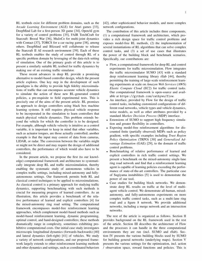
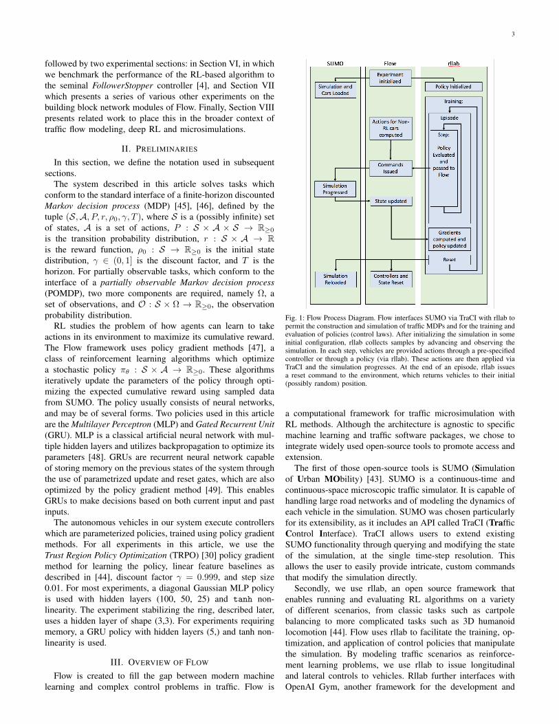
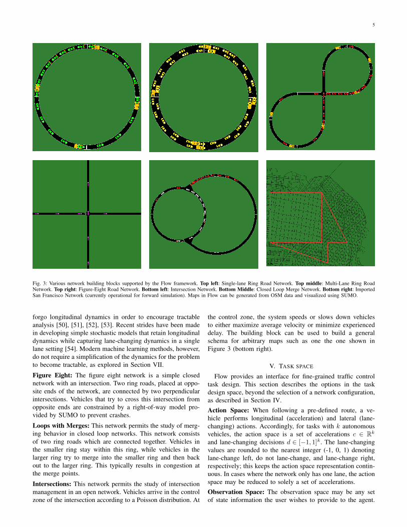
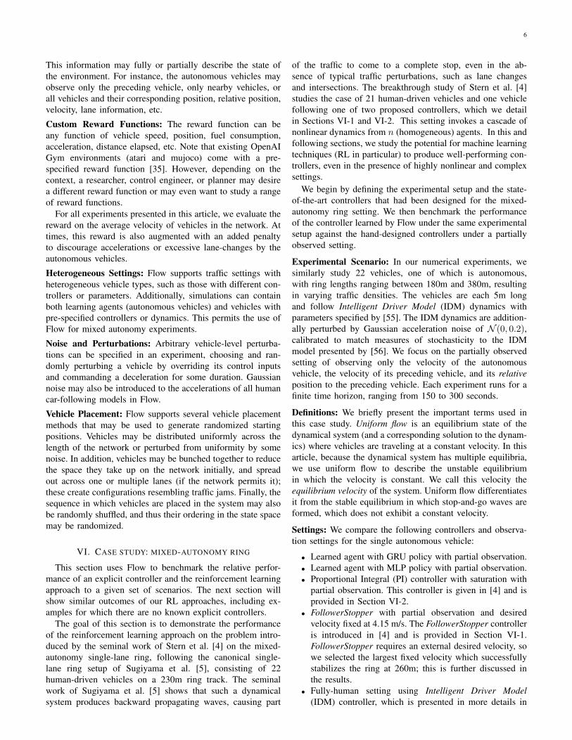
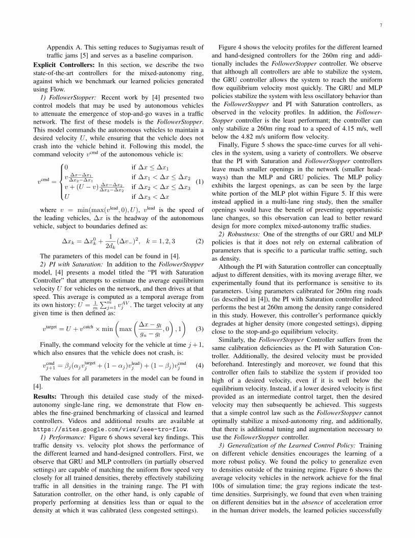

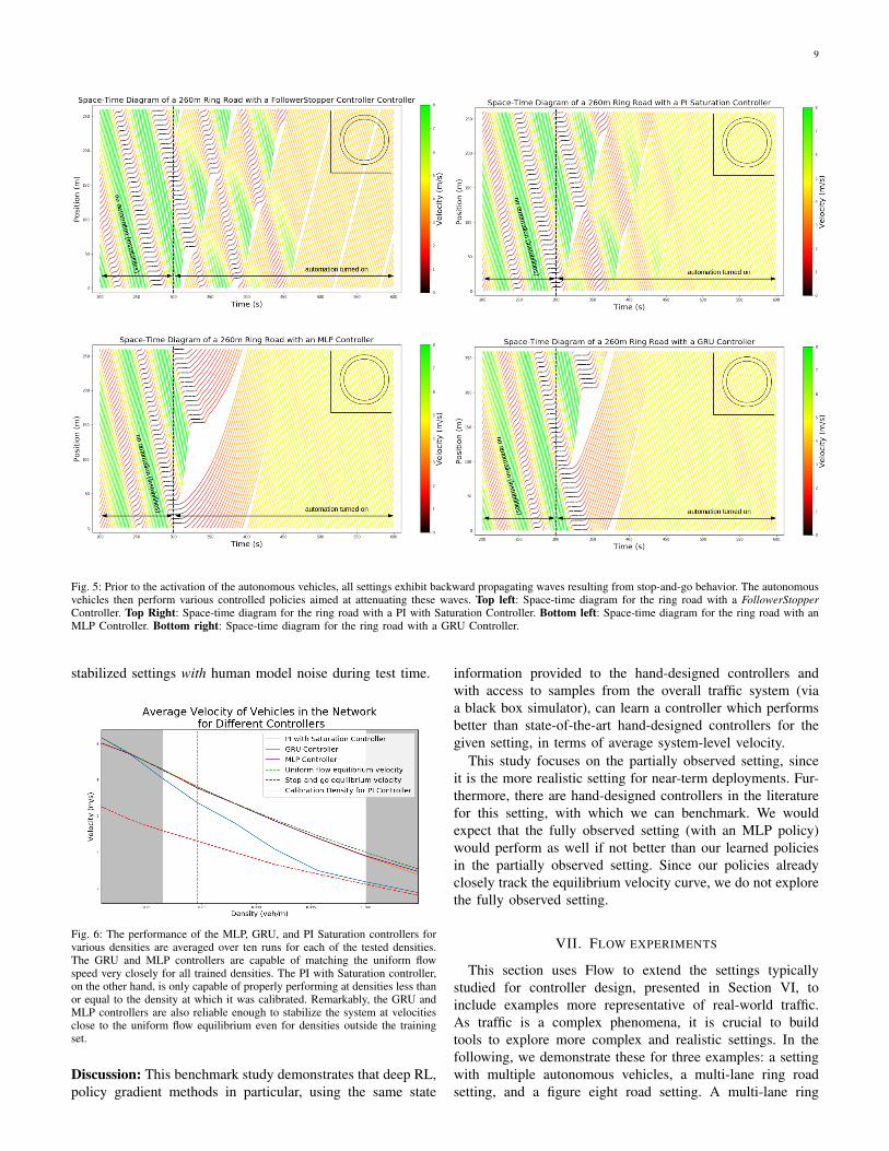
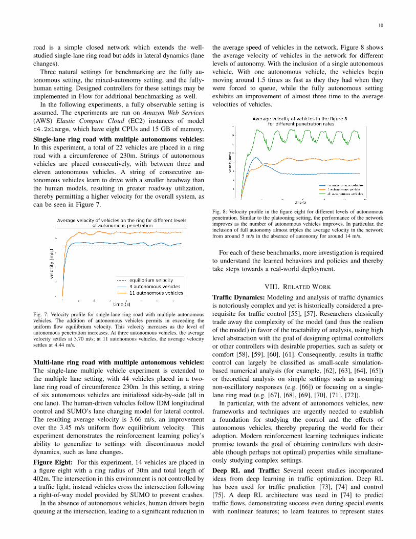
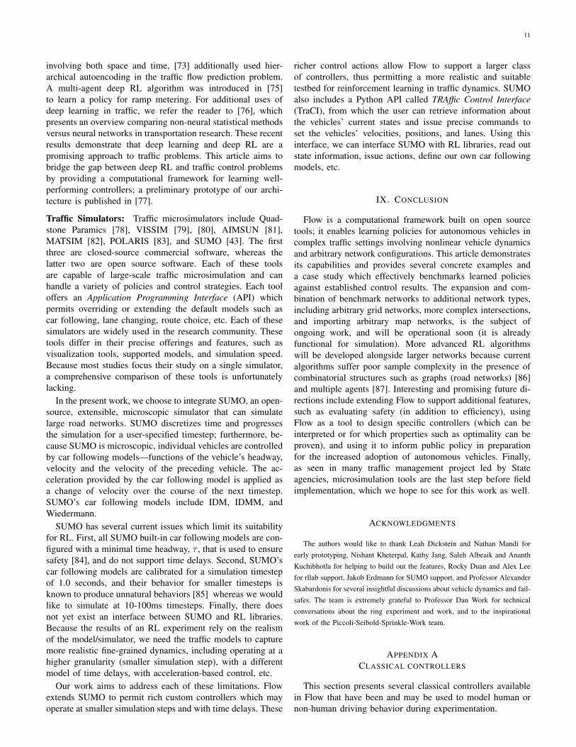

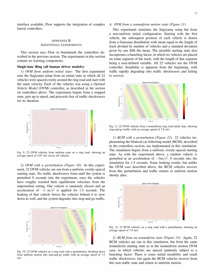


![POROUS MEDIA FLOW S - NSF REU: Interdisciplinary ...reu.cct.lsu.edu/documents/2014-posters/FortinoGarcia...BENCHMARKING PERFORMANCE OF POROUS MEDIA FLOW SIMULATIONS FORTINO GARCIA[1],](https://static.documents.pub/doc/80x56/60406c4fd62eca47e05f0ac0/porous-media-flow-s-nsf-reu-interdisciplinary-reucctlsuedudocuments2014-postersfortinogarcia.jpg)


