FLOW CONTROL AND SERVICE DIFFERENTIATION IN OPTICAL BURST SWITCHING NETWORKS a thesis submitted to the department of electrical and electronics engineering and the institute of engineering and sciences of bilkent university in partial fulfillment of the requirements for the degree of master of science By Hakan Boyraz April 2005
Transcript
FLOW CONTROL AND SERVICE
DIFFERENTIATION IN OPTICAL BURST
SWITCHING NETWORKS
a thesis
submitted to the department of electrical and
electronics engineering
and the institute of engineering and sciences
of bilkent university
in partial fulfillment of the requirements
for the degree of
master of science
By
Hakan Boyraz
April 2005
I certify that I have read this thesis and that in my opinion it is fully adequate,
in scope and in quality, as a thesis for the degree of Master of Science.
Asst. Prof Dr. Nail Akar(Supervisor)
I certify that I have read this thesis and that in my opinion it is fully adequate,
in scope and in quality, as a thesis for the degree of Master of Science.
Assoc. Prof. Dr. Ezhan Karasan
I certify that I have read this thesis and that in my opinion it is fully adequate,
in scope and in quality, as a thesis for the degree of Master of Science.
Prof. Dr. Erdal Arıkan
I certify that I have read this thesis and that in my opinion it is fully adequate,
in scope and in quality, as a thesis for the degree of Master of Science.
Assoc. Prof. Dr. Oya Ekin Karasan
I certify that I have read this thesis and that in my opinion it is fully adequate,
in scope and in quality, as a thesis for the degree of Master of Science.
Visiting Assoc. Prof. Dr. Tolga M. Duman
Approved for the Institute of Engineering and Sciences:
Prof. Dr. Mehmet BarayDirector of Institute of Engineering and Sciences
ii
ABSTRACT
FLOW CONTROL AND SERVICE
DIFFERENTIATION IN OPTICAL BURST
SWITCHING NETWORKS
Hakan Boyraz
M.S. in Electrical and Electronics Engineering
Supervisor: Asst. Prof Dr. Nail Akar
April 2005
Optical Burst Switching (OBS) is being considered as a candidate architecture
for the next generation optical Internet. The central idea behind OBS is the as-
sembly of client packets into longer bursts at the edge of an OBS domain and the
promise of optical technologies to enable switch reconfiguration at the burst level
therefore providing a near-term optical networking solution with finer switching
granularity in the optical domain. In conventional OBS, bursts are injected to
the network immediately after their assembly irrespective of the loading on the
links, which in turn leads to uncontrolled burst losses and deteriorating perfor-
mance for end users. Another key concern related to OBS is the difficulty of
supporting QoS (Quality of Service) in the optical domain whereas support of
differentiated services via per-class queueing is very common in current electroni-
cally switched networks. In this thesis, we propose a new control plane protocol,
called Differentiated ABR (D-ABR), for flow control (i.e., burst shaping) and
service differentiation in optical burst switching networks. Using D-ABR, we
show with the aid of simulations that the optical network can be designed to
work at any desired burst blocking probability by the flow control service of the
iii
proposed architecture. The proposed architecture requires certain modifications
to the existing control plane mechanisms as well as incorporation of advanced
scheduling mechanisms at the ingress nodes; however we do not make any spe-
cific assumptions on the data plane of the optical nodes. With this protocol, it is
possible to almost perfectly isolate high priority and low priority traffic through-
out the optical network as in the strict priority-based service differentiation in
electronically switched networks. Moreover, the proposed architecture moves the
congestion away from the OBS domain to the edges of the network where it is
possible to employ advanced queueing and buffer management mechanisms. We
also conjecture that such a controlled OBS architecture may reduce the number
of costly Wavelength Converters (WC) and Fiber Delay Lines (FDL) that are
used for contention resolution inside an OBS domain.
Keywords: Optical burst switching, rate control, service differentiation, conges-
tion control.
iv
OZET
OPTIK COGUSMA ANAHTARLAMALI AGLARDA AKIS
DENETIMI VE HIZMET AYRIMI
Hakan Boyraz
Elektrik ve Elektronik Muhendisligi Bolumu Yuksek Lisans
Tez Yoneticisi: Yard. Doc. Dr. Nail Akar
Nisan 2005
Optik Cogusma Anahtarlaması (OBS) gelecek nesil optik Internet icin aday
mimari olarak dusunulmektedir. OBS’ deki temel fikir istemci paketlerinin
giris dugumlerinde daha uzun cogusmalar seklinde toplanmasıdır. Cogusma
seviyesinde anahtarların yeniden duzenlesimine imkan tanıyarak optik ag
cozumlerini yakın gelecekte mumkun kılacak olan optik teknolojilerin umut
verici olması da bu fikri desteklemektedir. Alısılagelmis OBS’de, cogusmalar
olusturulduktan hemen sonra hatlardaki yuk yogunluguna bakılmaksızın optik
aga gonderilmektedir. Bu ise kontrolsuz cogusma kayıplarına ve son nokta kul-
lanıcıları icin performans bozukluguna neden olmaktadır. OBS ile ilgili diger
onemli bir problem ise gunumuz elektronik anahtarlama aglarında sınıfa dayalı
sıralama yontemi ile hizmet ayrımı desteginin cok yaygın olarak kullanılmasına
ragmen optik alanda hizmet ayrımı desteginin zor olmasıdır. Bu tezde, op-
tik cogusma anahtarlamalı aglarda akıs denetimi (cogusma sekillendirme) ve
hizmet ayrımı icin Ayrıstırmalı Izin Verilen Bit Hızı (D-ABR) olarak ad-
landırdıgımız yeni bir denetim duzlemi protokolu oneriyoruz. Onerdigimiz pro-
tokolun akıs kontrol hizmeti sayesinde optik bir agın istenilen cogusma kayıp
The rest of the thesis is organized as follows. In Chapter 2, we present an
overview of OBS and the existing mechanisms for service differentiation and
congestion control in OBS networks. We present the proposed OBS protocol for
congestion control and service differentiation in Chapter 3. Numerical results
are provided in Chapter 4. In the final chapter, we present our conclusions and
future work.
5
Chapter 2
Literature Overview
2.1 Optical Burst Switching (OBS)
Optical burst switching provides a granularity between packet switching and
wavelength switching [1]. In OBS, IP packets from different sources for the same
egress edge node are assembled into a burst at the ingress edge node. When the
burst arrives at the egress node, it is de-assembled back into IP packets and IP
packets are electronically routed to their destinations as shown in Fig. 2.1 [32].
When a burst is formed, a Burst Control Packet (BCP) is associated with it and
sent to the network in advance on a separate control channel. The control packet
is then processed electronically at each core node. According to the information
carried in the BCP, the resources are reserved for the burst and switch settings
are done beforehand.
The JET protocol is the most widely adopted reservation protocol for OBS
networks which does not require any kind of optical buffering at the intermediate
nodes. In JET-based OBS, a control packet is first sent towards the network over
the control channel to make a reservation for the burst. After an offset time, the
burst is sent to the core network without waiting for an acknowledgment for the
6
Edge Node
OBS Network
Toff
Control Channel
Data Channels
Access Network
Figure 2.1: OBS network architecture.
connection establishment, hence JET-based OBS uses the one-way reservation
mechanism unlike the wavelength switching case. Since switch settings are done
before the burst arrives, the burst passes through the network without requiring
O/E/O conversion and buffering. Fig. 2.2 depicts how the JET protocol operates
[1]. As we see in this figure, first the control packet is sent towards the network.
The control packet is then processed at the intermediate nodes and wavelength
reservation and switch settings are done. During this time, the burst is buffered
at the ingress node. After an offset time Toff , the burst is sent to the network
over the optical data channel. Suppose that the time required to process the
control packet and to configure the switch is 4 and the number of the hops to
the destination is H. Then, the offset time, Toff , should be chosen such that
Toff ≥ H4 to ensure that there is enough time for each intermediate node to
complete the processing of the control packet before the burst arrives [1]. Suppose
we set Toff = 34. Then, the total delay experienced by the burst in Fig. 2.2 is
P + 34 where P is the propagation delay.
7
Source DestinationOXC
2OXC
1
Burst
BCP
Toff
P
Toff
time
: Processing time at each node
Toff : Offset time
P : Propagation time
Figure 2.2: OBS with JET protocol.
In JET, BCP carries the offset time and burst length information in addition
to the usual control header data. The offset time field is used by intermediate
nodes to determine the arrival time of the burst. Since the time gap between the
BCP and the burst decreases when the BCP propagates through the network,
the offset time field is updated at each intermediate node as T ′off= Toff - 4. The
burst length information, which is carried by the BCP, enables the switches to
make close-ended reservations for bursts. Since the switch knows the exact arrival
and departure times of the bursts, it can take efficient reservation decisions which
can increase the bandwidth utilization and hence decrease the burst blocking
probability [1, 3].
Fig. 2.3 demonstrates how the switch can make use of the information on
burst start and end times [1]. In this figure, t′1 and t′2 are the arrival times of
BCPs for bursts 1 and 2, respectively, whereas t1 and t2 are the actual burst
arrival times. In both cases, the second burst will succeed in making reservation
if and only if the switch knows the arrival and departure times of both the first
and second bursts [3].
8
t1'
t2'
t1 t1+ l1
1st BCP 1st Burst
case 1case 2
2nd Burst
t2
X
Toff
Arrival Time
Figure 2.3: JET protocol with burst length information.
2.1.1 Burst Assembly
In OBS networks carrying IP traffic, IP packets from different sources for the
same egress node are aggregated into the same burst at the ingress node. This
procedure is called “burst assembly”. Fig. 2.4 shows the architecture of an ingress
edge node where burst assembly is carried out [3]. Packets with different priorities
are sent to different queues for burstification and the burst scheduler assembles
the packets from the same service category into bursts.
There are different methods proposed for the burst assembly (burstification)
procedure [3, 33]. One approach is “time-based assembly” in which a timer with
value T is set when the burst assembly starts and packets are aggregated into
a burst until the timer expires. In this type of burstification, the choice of T is
critical because when T is chosen large it increases the latency of the packets and
if it is short than many bursts with small sizes are generated which increases the
9
Packets tothe same
egress node
Class 1
Class N
Traffic fromEdge Routers
Burst Assembly Unit
Burst Assembly Unit
Burst Scheduler
Burst
BCP ControlPlane
QueueBurst
E/O
E/O
Figure 2.4: OBS ingress node architecture.
control overhead. Moreover, too small bursts require too fast switch reconfigura-
tions which may not be feasible by today’s switch fabrics. Another approach is
to use fixed burst lengths instead of fixed time intervals. In this method, packets
are aggregated into the same burst until the burst length reaches a predefined
minimum burst length. The drawback of this method is that when traffic rates
are low, then the burst assembly takes longer time and packets experience longer
delays. One approach is to combine these two methods dynamically according
to the real traffic measurements where a burst is formed when either a timer
expires or a predefined minimum burst length is reached [33].
When the burst assembly procedure is completed, a BCP is sent towards
the network to request a resource reservation for the burst. The actual burst
is delayed by an offset time before being transmitted to the network. When
the burst is queued up at the ingress node after the BCP is sent, the potential
incoming packets in the meantime cannot be included in the current burst since
the BCP already contains the length of the burst when it is sent to the network.
10
In order to reduce the delay experienced by newly incoming packets, a predicted
burst length may be used in the BCP instead of the actual burst length, i.e.
l + f(t) where l is the actual burst length and f(t) is the predicted increase
in the burst length during the offset time [3]. After the offset time if the final
burst length is shorter than the predicted one, then some of the resources will
be wasted and otherwise then only a small number of packets will have to wait
for the next burst.
2.1.2 Contention Resolution
When multiple bursts contend for the same outgoing wavelength, a contention is
said to occur. Basically there are three ways of resolving contention [32]:
• Wavelength Domain: The contending bursts can be sent on a different
wavelength channel of the designated output link by using wavelength con-
verters. The switch may have Full Wavelength Conversion (FWC) capabil-
ity or Partial Wavelength Conversion (PWC) capability. In FWC, a burst
arriving at a certain wavelength can be switched onto any other wavelength
towards its destination. In Partial Wavelength Conversion (PWC), there
is a limited number of converters which are shared among all wavelengths,
and consequently some bursts cannot be switched towards their destination
(and therefore blocked) when all converters are busy despite the availability
of free channels on wavelengths different from the incoming wavelength [5].
• Time Domain: Contention may be resolved in time domain by delaying the
contending bursts until the contention is resolved by using FDLs. FDLs
provide only a fixed amount of delay unlike the electronic buffers. Different
optical buffering approaches are suggested by using FDLs. Optical buffers
may be categorized in terms of the number of the FDL stages; i.e, single-
stage or multistage, and in terms of the used buffering configuration; i.e,
11
Feed-Forward (FF) or Feedback (FB) configuration [34]. In FF configura-
tion, each FDL forwards the optical packet (or the burst in OBS) to the
next stage of the switch whereas in the FB configuration the packet is sent
back to the input of the same stage.
• Space Domain: In the space domain contention resolution scheme, one
of the contending bursts is sent through an another route to the desti-
nation which is also called “deflection routing”. In OBS, the deflection
route should be determined beforehand and the offset time should be cho-
sen to compensate for the extra processing time encountered by the BCP.
Moreover, use of deflection routing may occasionally degrade the system
efficiency unexpectedly because deflected bursts may cause contention else-
where.
The OBS switch may use a combination of the above methods to resolve
contention. The effect of using FDLs and WCs on burst blocking probability
is studied in [32]. It is shown that using FDLs with lengths equal to a few
mean burst lengths performs well in terms of blocking probability. Increasing
the number of FDLs is also shown to reduce the burst blocking probabilities, as
would be expected [32].
When contention cannot be resolved by using at least one of the above meth-
ods, the contending burst will be dropped. In [35], a new contention resolution
technique called “burst segmentation” is proposed to reduce burst losses. In this
method, bursts are divided into segments where a segment may contain one or
more data packets and when contention occurs only the contending segments
are dropped instead of dropping the complete burst. Different approaches exist
depending on which part of the burst is to be dropped [35]. One approach is
to drop the tail of the original burst and another is to drop the head of the
contending burst.
12
2.1.3 Burst Scheduling Algorithms
When a BCP arrives at the switch, a burst scheduling algorithm is run to assign
one of the available wavelengths to the incoming burst assuming the availability
of wavelength converters. Different burst scheduling algorithms are proposed in
the literature. Some of these algorithms are summarized in [3]. A burst which has
been assigned a wavelength is called a scheduled burst whereas the incoming burst
that is not scheduled yet is called an unscheduled burst. Following algorithms
are proposed for burst-scheduling in the literature [3]:
• Horizon / Latest Available Unscheduled Channel (LAUC): The horizon of
a wavelength is defined as the latest time at which the wavelength will be in
use. The LAUC algorithm chooses the wavelength channel with minimum
horizon that is less than the start time of the unscheduled burst. Since this
approach does not make use of the gaps between scheduled bursts, it is not
considered to be a bandwidth-efficient algorithm.
• LAUC with Void Filling (LAUC-VF): This algorithm makes use of the gaps
between scheduled bursts. There are many variants of this algorithm such
as Min-SV (Starting Void), Min-EV (Ending Void), and Best Fit. In Min-
SV, the algorithm chooses the wavelength among available wavelengths
for which the gap between the end of the scheduled burst and the start
of the unscheduled burst is minimum. Min-EV tries to minimize the gap
between the end of the unscheduled burst and the start of the scheduled
burst. Finally, Best Fit algorithm tries to minimize the total length of the
starting and ending voids that would be introduced after reservation.
Fig. 2.5 depicts which channels would be scheduled with different scheduling
algorithms [3]. Ci is the ith wavelength on the output link, ts and te are the start
and end times of the unscheduled burst respectively. As shown in the figure, if
the horizon algorithm is used then C3 will be chosen because it has the earliest
13
New Burst
C1 Min-SV
C2
C3 Horizon
C4 Min-EV
C5 Best Fit
Time
t1 t'1 t''1
t2 t'2
t3
t''2
t4 t''4t'4
t5 t'5 t''5
tS te
Figure 2.5: Working principles of different scheduling algorithms.
horizon time among the channels. If min-SV algorithm is used, then C1 will be
chosen for which the gap between the starting time of the incoming burst and
the end time of the scheduled burst, i.e. ts − t1, is minimum among candidates.
Similarly, C4 will be chosen for the Min-EV algorithm and C5 will be chosen for
the Best Fit algorithm. C2 will not be chosen in any case since the scheduled
burst is in conflict with the incoming burst.
When there are FDLs as well, further scheduling algorithms can also be in-
troduced to take advantage of FDLs [36, 37].
2.1.4 Service Differentiation in OBS Networks
One approach to manage QoS in OBS networks is to use different offset times
for different classes of bursts [20]. In OBS, recall that a burst is sent after the
14
BCP by an offset time so that the wavelength is reserved and switch settings are
done before the burst arrives.
Offset time based QoS schemes assign extra offset times to high priority class
bursts. To show how this scheme works, suppose that there are two classes of
traffic i.e., classes 0 and 1 where class 0 bursts have lower priority than class 1
bursts [20]. Let tia be the arrival time of the class i request denoted by req(i),
tis be the arrival time of the corresponding burst, li be the length of the req(i)
burst and finally let tio be the offset time assigned to the class i burst. Without
loss of generality suppose that the offset time for class 0 bursts is 0 and an extra
offset time, denoted by t1o, is given to class 1 bursts. Therefore, t1s = t1a + t1o and
t0s = t0a. First suppose that a high priority burst request arrives and makes the
reservation for the wavelength as shown in Fig. 2.6a. After the class 1 request, a
class 0 request arrives and attempts to make a reservation. From Fig. 2.6, req(1)
will always succeed in making a reservation but req(0) will succeed only when t0s
< t1s and t0a + l0 < t1s or t0s > t1s + l1, otherwise it will be blocked.
In the second case, req(0) arrives first and makes a reservation as shown in
Fig. 2.6b. After req(0), req(1) arrives and attempts to make the reservation for
the corresponding class 1 burst. When t1a < t0a + l0, req(1) would be blocked if no
extra offset time had been assigned to req(1). But with extra offset time, it can
accomplish successful reservation if t1a + t1o > t0a + l0. In the worst case, suppose
that req(1) arrives just after the arrival of req(0), then req(1) will succeed only
if the offset time is longer than the low priority burst size. Hence, class 1 bursts
can be completely isolated from class 0 bursts by choosing the extra offset time
assigned to the high priority bursts long enough.
In [21] and [22], a QoS scheme with extra offset time is studied with FDLs.
The offset time required for class isolation when making both wavelength and
FDL reservations is quantified. When there are FDLs, how the class isolation is
maintained and how the offset time should be chosen is presented in this study.
15
(a)
ts1
iTime
ts1 + l1ta
1
to1
ta0 ( = ts
0 )
(b)
ts1
iTime
ts0 + l0ta
1
to1
ta0 ( = ts
0 )
Figure 2.6: Class isolation without FDLs.
To see how the class isolation is provided when there are FDLs, suppose that
there are two traffic classes as in the previous example and offset time for class
0 traffic is again 0. But this time suppose that there is only one single fiber
delay line, which can provide a variable delay between 0 and B [21]. In the
first case, suppose that when req(0 ) arrives at t0a the wavelength is in use by an
another burst as shown in Fig. 2.7a. Therefore, if there were not FDLs it would
be blocked, but with FDLs if the amount of the delay required t0b is less than
B then the FDL is reserved for the class 0 burst as shown in Fig. 2.7b and the
wavelength is reserved for the class 0 burst from t = t0s + t0b till t = t0s + t0b + l0.
Now assume that req(1) arrives as shown in Fig. 2.7a. If the offset time assigned
to class 1 bursts is long enough i.e., t1a + t1o > t0s + t0b + l0, then it will succeed to
make a reservation. If the offset time assigned to class 1 bursts is not long enough
to make a wavelength reservation successfully, then req(1) needs to reserve the
FDLs. In this case if t1a + t1o > t0s + l0 then req(1) reserves the FDL successfully.
16
Figure 2.7: Class isolation at an optical switch with FDLs.
Finally, assume that req(1) arrives before req(0) as shown in Fig. 2.7c., then it
reserves the wavelength without being affected by req(0). The class 0 request
will succeed in reserving wavelength only if t0s + l0 < t1a + t1o. Again we see that
by choosing offset times appropriately, class 1 bursts can perfectly be isolated
from class 0 bursts in both reserving wavelengths and FDLs. Additional QoS
classes can be introduced by incorporating additional offset times to the new
QoS classes.
Table 2.1 shows how extra offset time effects the class isolation. L is the mean
burst length of class 0 bursts where burst lengths are exponentially distributed
[21]. R is the degree of the isolation between classes i.e. probability that a
17
class 1 burst will not be blocked by a class 0 burst, B is the maximum amount
of the delay provided by FDLs. Giving sufficiently large extra offset times to
higher priority bursts can provide sufficient isolation between classes but these
extra offset times increase the end-to-end delay of the network which is a critical
design parameter for real time applications. Also degree of the isolation depends
on burst length and interarrival time distributions. Finally, the differentiation is
not even among classes i.e. the ratio of class i loss probability to the class 0 loss
probability is not equal to the ratio of class i − 1 loss probability to the class 0
loss probability.
R 0.6321 0.9502 0.9932
toffset ( FDL ) L 3.L 5.Ltoffset (λ) L + B 3.L + B 5.L + B
Table 2.1: Relation between extra offset time and degree of isolation.
Another approach similar to offset time based QoS is given in [28] but this
approach does not use extra offset times. The authors propose a linear predic-
tion filter (LPF) based forward reservation method to reduce end-to-end delays
and also provide QoS. In this method, normal resource reservation procedure is
implemented for low priority traffic (class 0 traffic) where BCP is sent to the core
network after the completion of burst assembly and it contains the actual burst
length. For high priority bursts (class 1 traffic), the BCP is sent before burst as-
sembly completion by a time Tp and it contains the predicted burst length, which
is obtained by a LPF. After the burst assembly, if the actual burst length is less
than the predicted burst length then the BCP pre-transmission is supposed to be
successful and the burst is sent to the core network just after the burst assembly
completion as shown in Fig. 2.8 where Tb is the time when the burst assembly
starts, la is the length of the burst, T ih is the time when BCP is transmitted for
class i traffic, T id is the time when the class i burst is transmitted to the core
network. If the actual burst length is larger than the predicted burst length,
18
To
Tb la
Th1 Td
1
Tp
time
Th0 Td
0
To
Figure 2.8: FFR based QoS example.
the BCP pre-transmission deemed a failure and BCP has to be retransmitted
after burst assembly. End-to-end delay of the high priority bursts is reduced by
this method. However, when the pre-transmission fails (predicted burst length
is larger than the actual burst length), class isolation also fails. On the other
hand if the predicted burst length is shorter than the actual burst length then
resources are wasted. Moreover, the QoS design parameter Tp strictly depends
on burst the length distribution.
In [23], a controllable QoS differentiation, namely Proportional QoS, on delay
and burst loss probability without extra offset times is offered. In proportional
QoS, an intentional burst dropping scheme is used to provide proportionally
differentiated burst loss probability and a waiting time priority (WTP) scheduler
is used to provide proportionally differentiated average packet delay.
In intentional burst dropping scheme, burst loss rates of each class are con-
stantly calculated at each switch and low priority bursts are intentionally dropped
to maintain proportional data loss between classes. This gives longer free time
periods on the output link capacity, which increases the probability of high prior-
ity bursts to be admitted. This method provides proportionality between burst
loss rates of different classes of traffic and proportionality factor can be used as
a design parameter [23].
19
Figure 2.9: WTP edge scheduler.
In the WTP Scheduler, there is a queue for each class of traffic as shown in
Fig. 2.9. A burst is formed and transmitted when a token is generated. Token
generation is a Poisson process. Priority of each queue is calculated as pi(t) =
wi(t)/si where wi(t) is the waiting time of the packet at the head of queue i and
si is the proportionality factor for class i. The queue with the largest pi(t) is
chosen for burst assembly. By this way, proportional average packet delays are
maintained among classes [23].
In intentional burst dropping an arriving burst is dropped if its predefined
burst loss rate is violated regardless of the availability of the wavelength. This
gives more free times on the wavelength for high priority bursts but it leads to
higher burst blocking probabilities and also worsens wavelength utilization.
Another approach is to use soft congestion resolution techniques in QoS sup-
port [24, 25, 26, 27]. In [24], authors suggest a QoS scheme, which combines
prioritized routing and burst segmentation for differentiated services in optical
network. When multiple bursts contend for the same link, a contention occurs.
One way of the contention resolution is deflection routing in which the contend-
ing burst is routed over an alternative path. When the choice of the burst that
will be deflected is based on priority then it is called as prioritized deflection.
When contention cannot be resolved by traditional methods such as wavelength
20
conversion, deflection routing etc. one of the bursts is dropped completely. Burst
segmentation is suggested to reduce packet losses during a contention. In burst
segmentation instead of dropping the burst completely only the overlapping pack-
ets are dropped [31]. To further reduce the packet losses, the overlapping packets
may be deflected. QoS is provided by selectively choosing the bursts that will
be segmented or deflected. In [24] authors define three policies for handling
contention. These are:
• Segment First and Deflect Policy (SFDP): Original burst is segmented
and its overlapping packets are deflected if an alternate port is available
otherwise the tail is dropped.
• Deflect First and Drop Policy (DFDP): Contending burst is deflected if
possible otherwise it is dropped.
• Deflect First, Segment and Drop Policy (DFSDP): Contending burst is de-
flected to an alternate port if available otherwise original burst is segmented
and its tail is dropped.
Table 2.2 is given in [24] to show how the above policies can be used to provide
QoS. Longer remaining burst column in Table 2.2 shows, after segmentation
which one of the bursts has longer remaining data. Authors show that the loss
rate and delay of the high priority bursts are less than the corresponding low
priority values by simulations.
In [25], a burst assembly and scheduling technique is offered for QoS support
in optical burst switched networks. In this method, packets from different classes
are assembled into the same burst such that the priority of the packets decreases
towards the tail of the burst. When contention occurs, the original burst is
segmented so that the tail is dropped. Since the packets at the tail have lower
priority than the packets at the head of the burst, the loss rate of the high priority
packets is reduced.
21
Condition Original Contending Longer PoliciesBurst Priority Burst Priority Remaining Burst
1 High High Contending DFSDP2 High Low Contending DFDP3 Low High Contending SFDP4 Low Low Contending DFSDP5 High High Original DFDP6 High Low Original DFDP7 Low High Original SFDP8 Low Low Original DFDP
Table 2.2: QoS policies for different contention situations.
Another contention resolution technique with QoS support is given in [26].
This method is suggested for slotted OBS networks where control and data chan-
nels are divided into fixed time slots and bursts are sent only at time slot bound-
aries. At the optical core node, all the BCPs destined to the same output port
are collected for a time period of W and a look-ahead window is obtained. Then,
contention regions are determined in the corresponding burst window. By ap-
plying a heuristic algorithm, the bursts that should be dropped within a data
window are determined. Priority and length of the bursts are used as parame-
ters in the algorithm. The authors of [26] suggest that either partial or absolute
differentiation can be provided. In partial differentiation, a high priority burst
with a short length can be blocked by a low priority burst with a longer length.
The problem with this algorithm is that BCPs should be stored for duration of
W time units before they are transmitted and FDLs should be used at each hop
to delay bursts by W to maintain original offset times. Moreover, the end-to-end
data delay increases as the window size increases. To maintain a low end-to-end
delay, W should be kept small but this time the performance of the algorithm
degrades.
In [29], a preemptive wavelength reservation mechanism is introduced to pro-
vide proportional QoS. To see how it works assume that there are N classes
22
c1, c2,. . . , cN where c1 has the lowest priority and cN has the highest priority.
A predefined usage limit is assigned to each class of traffic i.e., pi such that∑N
i=1 pi = 1. At each switch, following data is held for each class of traffic:
• Predefined usage limit
• Current usage
• A list of scheduled bursts within the same class, start and stop times of
the reservations for the bursts and a predefined timer for each reservation
Current usage of the class i, ri, is calculated over a short time period t. It
is the total reservation time of class i bursts over the total reservation time of
the bursts of all classes. A class is said to be in profile if current usage is less
than the predefined usage limit otherwise it is said to be out of profile. When
a new request cannot make a reservation, a list is formed which contains the
classes whose priorities are less than the priority of the current request and
whose current usages exceed their usage limits. Then the switch checks whether
the new request can be scheduled by removing one of the existing requests in
the list beginning from the lowest priority request. If such an existing request is
found, it is preempted and the switch updates the current usage of both classes.
When a reservation is preempted, two methods are used to prevent wasting of
resources at downstream nodes. If the burst is preempted during transmission,
the switch stops the burst transmission and sends a signal at the physical layer
indicating the end of burst. In the other situation, a downstream node can use
a predefined timer for each reservation, which is activated at the requested start
time of the burst. If the burst does not arrive before the timer expires then the
switch decides on the occurrence of a fault and cancels the reservation for this
burst.
All the above existing QoS schemes provide a level of isolation between QoS
classes but it is not clear whether the isolation is in the strict-priority sense.
23
Moreover, these existing proposals do not attempt to ensure fairness among the
competing connections. In this thesis, we study the support of strict priority-
based service differentiation in OBS networks while maintaining perfect isolation
between high and low priority classes. Another dimension of our research is fair
allocation of bandwidth among contending connections.
2.1.5 Flow Control in OBS Networks
In all the QoS schemes mentioned in the previous section, how the burst loss
rate for high priority bursts can be reduced has been studied. However, when
the network is heavily congested, then burst losses will also be very high for
high priority traffic bursts and the QoS schemes of the previous section would
not work properly. In order to prevent the network entering into a congestion
state where bursts losses are high, contention avoidance policies can be used.
Contention avoidance policies can be non-feedback based or feedback based. In
non-feedback based congestion control, the edge nodes regulate their traffic ac-
cording to a predefined traffic descriptor or some stochastic model. In feedback-
based congestion avoidance algorithms, sources dynamically shape their traffic
according to the feedback returned from the network.
In the following studies, a number of congestion control mechanisms for op-
tical burst switched networks have been proposed. In [39], a feedback-based
congestion avoidance mechanism called as Source Flow Control (SFC) is intro-
duced. In this proposed mechanism, the optical burst switches send explicit
messages to the source nodes to reduce their rates on congested links. Core node
switches measure the load at their output ports. If the calculated load is larger
than the target load then they broadcast a flow rate reduction (FFR) request
besides the label of the lightpath and the core switch address where the conges-
tion occurs. FFR has two fields: control field and rate reduction value field. In
the control field there are two flags: idle flag and no increase flag. When the idle
24
Regulated Burst Transmission
Admission ControlBurst AssemblyModule
FFR from the corenetwork
Rate Controlleron link (i,j)
Buffer Bi,j
Arrival rate: ij
Bursts passing throughlink (i,j)
Ti,j
Figure 2.10: Source flow control mechanism working at edge nodes.
flag is set sources can increase their rates, when no increase flag is set sources
are not allowed to increase their current rates. Rate reduction field shows the
rate reduction value, Rij, required on link (i, j). It is calculated as follows:
Rij = ρ−ρthρth
where ρ is the actual traffic load on link (i, j) and ρth is the target
load on link (i, j). The core switch address where the contention occurs is also
sent to the ingress nodes so that the ingress node can use an alternative path to
the congested path. When sources receive the FFR message and if the rate re-
duction field is set then they decrease their current rates using link (i, j) as stated
in FFR. The actual rates are stored to be used when congestion disappears. An
admission control is used to send the bursts at the determined rate. Authors
suggest using timers such that when a burst is transmitted a timer is set whose
value is equal to the inverse of the required transmission rate. When the timer
expires, a new burst is sent as shown in Fig. 2.10. When the contention disap-
pears on link (i, j), the sources return their original rates using a random delay.
In this type of admission control burst rates are adjusted assuming that burst
lengths are constant. The rates are not explicitly declared for each source but
only the overload factor is sent to the sources and the fairness among sources is
not tested. Also no service differentiation mechanism is offered in this congestion
control mechanism.
25
Another congestion control algorithm for OBS networks is given in [30]. In
this algorithm the intermediate nodes send the burst loss rate information to all
edge nodes so that they can adjust their rates to hold the burst loss rate at a
critical value. For all edge nodes the maximum amount of traffic that the node
can send, i.e. critical load, to the network in case of heavy traffic is determined
offline. By analyzing the burst loss rates returned from switches, edge nodes
determine whether the network in heavy load situation or not. If the network is
congested then an edge node decides on its transmission rate as follows:
• If its current load is less than its critical load then it can increase its rate
if needed
• If its current load is greater than its critical load then it reduces its trans-
mission rate
• If its current load is equal to its critical load it does not change its rate
This method guarantees a minimum bandwidth to each edge node. Also
when an edge node does not use its bandwidth, other edge nodes can share this
bandwidth but it is not clear that the bandwidth can be fairly shared between
edge nodes. Authors of [30] also suggest a burst retransmission scheme which is
invoked when an edge node receives a negative acknowledge (NACK) from the
core network which shows a burst drop. This scheme works as follows:
• When an ingress node transmits a burst, keeps its copy and sets a timer
• If the ingress node receives a NACK for this burst, it retransmits the burst
and sets the timer again
• If the timer expires the ingress node supposes that the burst is transmitted
successfully and deletes the copy of the burst.
26
Using this scheme, the OBS network is shown in [30] to respond to burst losses
quickly.
27
Chapter 3
Differentiated ABR
We envision an OBS network comprising edge and core OBS nodes. A link be-
tween two nodes is a collection of wavelengths that are available for transporting
bursts. We also assume an additional wavelength control channel for the con-
trol plane between any two nodes. Incoming IP packets to the OBS domain are
assumed to belong to one of the two classes, namely High-Priority (HP) and
Low-Priority (LP) classes. For the data plane, ingress edge nodes assemble the
incoming IP packets based on a burst assembly policy (see for example [12])
and schedule them toward the edge-core links. We assume a number of tune-able
lasers available at each ingress node for the transmission of bursts. The burst de-
assembly takes place at the egress edge nodes. We suggest to use shortest-path
based fixed routing under which a bi-directional lightpath between a source-
destination pair is used for the burst traffic. We assume that the core nodes do
not support deflection routing but they have PWC and FDL capabilities on a
share-per-output-link basis [13].
The proposed architecture has the following three central components [40]:
• Off-line computation of the effective capacity of optical links,
28
• D-ABR protocol and its working principles,
• Algorithm for the edge scheduler.
3.1 Effective Capacity
Let us focus on an optical link with K wavelength channels per link, each channel
capable of transmitting at p bits/s. Given the burst traffic characteristics (e.g.,
burst interarrival time and burst length distributions) and given a QoS require-
ment in terms of burst blocking probability Ploss, the Effective Capacity (EC)
of this optical link is the amount of traffic in bps that can be burst switched by
the link while meeting the desired QoS requirement. In order to find the EC
of an optical link, we need a burst traffic model. In our study, we propose the
effective capacity to be found based on a Poisson burst arrival process with rate
λ (bursts/s), an exponentially distributed burst service time distribution with
mean 1/µ (sec.), and a uniform distribution of incoming burst wavelength. Once
the traffic model is specified and the contention resolution capabilities of the
optical link are given, one can use off-line simulations (or analytical techniques
if possible) to find the EC by first finding the minimum λmin that results in
the desired blocking probability Ploss and then setting EC = λminp/µ. We note
that improved contention resolution capability of the OBS node also increases
the effective capacity of the corresponding optical link. We study two contention
resolution capabilities in this paper, namely PWC and FDL. In PWC, we assume
a wavelength converter bank of size 0 < W ≤ K dedicated to each fiber output
line. Based on the model provided in [5], a new burst arriving at the switch on
wavelength w and destined to output line k
• is forwarded to output line k without using a Tune-able Wavelength Con-
verter (TWC) if channel w is available, else
29
• is forwarded to output line k using one of the free TWCs in the converter
bank and using one of the free wavelength channels selected at random,
else
• is blocked.
An efficient numerical analysis procedure based on blocktridiagonal LU fac-
torizations is given in [5] for the blocking probabilities in PWC-capable optical
links and therefore the EC of an optical link can very rapidly be obtained in
bufferless PWC-capable links.
We study the case of L FDLs per output link where the ith FDL, i = 1, 2, . . . ,
L can delay the burst bi = i/µ sec. The burst reservation policy that we use is
to first try wavelength conversion for contention resolution and if conversion fails
to resolve contention we attempt to resolve it by suitably passing a contending
burst through one of the L FDLs. To the best of our knowledge, no exact
solution method exists in the literature for the blocking probabilities in OBS
nodes supporting FDLs and therefore we suggest using off-line simulations in the
latter scenario to compute the EC of FDL-capable optical links. The optical link
model using PWC and FDLs that we use in our simulation studies is depicted in
Fig. 3.1.
3.2 D-ABR Protocol
The feedback information received from the network plays a crucial role in our
flow control and service differentiation architecture. Our goal is to provide flow
control so as to keep burst losses at a minimum and also emulate strict priority
queueing through the OBS domain. For this purpose, we propose that a feedback
mechanism similar to the ABR service category in ATM networks is to be used in
OBS networks as well [14]. In the proposed architecture, the ingress edge node of
30
Wavelength ConverterBank
b1
bL
b2
Output FibersInput Fibers
1
K
1
K
1
K
1
K
1
K
1
K
1
2
N
1
2
M
1
2
W
FDLBuffer
Figure 3.1: The general architecture of the OBS node under study.
31
bi-directional lightpaths sends Resource Management (RM) packets with period
T sec. in addition to the BCPs through the control channel. These RM packets
are then returned back by the egress node to the ingress node using the same
route due to the bidirectionality of the established lightpath. Similar to ABR,
RM packets have an Explicit Rate (ER) field but we propose for OBS networks
one separate field for HP bursts and another for LP bursts. RM packets also have
fields for the Current Bit Rate (CBR) for HP and LP traffic, namely HP CBR
and LP CBR, respectively. This actual bit rate information helps the OBS nodes
in determining the available bit rates for both classes. On the other hand, the
two ER fields are then written by the OBS nodes on backward RM packets using
a modification of ABR rate control algorithms, see for example the references for
existing rate control algorithms [15, 16, 17].
In our work, we choose to test the basic ERICA (Explicit Rate Indication
for Congestion Avoidance) algorithm due to its simplicity, fairness, and rapid
transient performance [10]. Moreover, the basic ERICA algorithm does not use
the queue length information as other ABR rate control algorithms do, but this
feature turns out to be very convenient for OBS networks with very limited
queueing capabilities (i.e., limited number of FDLs) or none at all. We leave a
more detailed study of rate control algorithms for OBS networks for future work
and we outline the basic ERICA algorithm and describe our modification to this
algorithm next in order to mimic the behavior of strict priority queuing.
We define an averaging interval Ta and an ERICA module for each output
port. An ERICA module has two counters, namely the HP counter and the LP
counter, to count the number of bits arriving during an averaging interval. These
counters are updated whenever a burst arrives to the output port as follows:
if an HP burst arrives then,
HP Counter = HP Counter + Burst Size,
else
32
LP Counter = LP Counter + Burst Size.
The counters are used to find the HP and LP traffic rates during an averaging
interval. The pseudo-code of the algorithm that is run by the OBS node at the
end of each averaging interval is given in Fig. 3.2. The EC of the link is the
capacity that HP traffic can use. The remaining capacity is up for use for LP
traffic.The parameter a in Fig. 3.2 is used to smooth the capacity for LP traffic.
In our work we have used a = 1. The load factors and fair shares for each class
of traffic are then calculated along the lines of the basic ERICA algorithm [10].
All the variables set at the end of an averaging interval will then be used for
setting the HP and LP Explicit Rates (ER) upon the arrival of backward RM
cells within the next averaging interval. Note that all the information used in
this algorithm is available at the BCPs and therefore the algorithm runs only at
the control plane.
The algorithm to be used for calculating the explicit rates for the lightpath is
run upon the arrival of a backward RM cell. The pseudo-code for the algorithm
is depicted in Fig. 3.3. The central idea of the basic ERICA algorithm is to
achieve fairness and high utilization simultaneously whereas with our proposed
modification we also attempt to provide isolation between the HP and LP traf-
fic. The load factors in the algorithm are indicators of the congestion level of
the link [10]. High overload values are undesirable since they indicate excessive
utilization of the link. Low overload values are also undesirable since they in-
dicate the underutilization of the link. The optimum operating point is around
unity load factor. The switch allows the sources that transmit at a rate less than
FairShare to raise their rates to FairShare every time it sends a feedback to
a source [10]. If a source does not use its FairShare completely, the remaining
capacity is shared among the sources which can use it. LightpathShare in the
algorithm is used for this purpose. LightpathShare tries to bring the network to
an efficient operating point, which may not be necessarily fair. Combination of
these two quantities brings the network to the optimal operation point rapidly.
33
At the end of averaging interval
Calculate number of active HP lightpaths (N_HP) in the lastinterval
Calculate number of active LP lightpaths (N_LP) in the lastinterval
ABR Capacity := Target Utilization x Effective Capacity
HP Input Bit Rate := HP Counter / Averaging Interval
LP Input Bit Rate := LP Counter / Averaging Interval
HP Load Factor := HP Input Rate / HP Capacity
HP Fair Share := HP Capacity / N_HP
LP Fair Share := LP Capacity / N_LP
Reset HP Counter
Reset LP Counter
Reset number of active lightpaths
HP Capacity := ABR Capacity
LP Capacity := ABR Capacity -
[a x HP Input Bit Rate+(1-a) x HP Input Rate at previous interval ]
LP Capacity := max(0,LP Capacity)
If LP Capacity > 0
LP Load Factor := LP Input Rate / LP Capacity
LP Load Factor := 0
YES
NO
Figure 3.2: Proposed algorithm to be run by the OBS node at the end of eachaveraging interval.
34
On receiving a backward RM packet
Lightpath HP Share := HP CBR / HP Load Factor
if HP Load Factor > 0Lightpath HP Share := 0
if LP Load Factor > 0
Lightpath LP Share := LP CBR / LP Load Factor
Lightpath LP Share := 0
HP ER := max( HP Fair Share, Lightpath HP Share )
LP ER := max( LP Fair Share, Lightpath LP Share )
HP (LP) ER > HP (LP) FairShareand
HP (LP) CBR < HP (LP) FairShare
HP(LP) ER := HP(LP) Fair Share
HP ER := min( HP ER, HP Capacity )
LP ER := min( LP ER, LP Capacity )
HP ER in RM := min( HP ER, HP ER in RM )
LP ER in RM := min( HP ER, LP ER in RM )
YES
YES
YES
NO
NO
NO
Figure 3.3: Proposed algorithm to be run by the OBS node upon the arrival ofa backward RM packet.
35
The calculated ER cannot be greater than the effective capacity of the link and
it is checked in the algorithm as shown in Fig. 3.3. Finally, to ensure that the
bottleneck ER reaches the source, the ER field of the BCP is replaced with the
calculated ER at a switch only if the switch’s ER is less than the ER value in
the BCP [10]. Having received the information on HP and LP explicit rates, the
sending source decides on the Permitted Bit Rate (PBR) for HP and LP traffic,
namely HP PBR and LP PBR, respectively. These PBR parameters are updated
on the arrival of a backward RM packet at the source:
HP PBR := min(HP ER, HP PBR + RIF*HP PBR),
LP PBR := min(LP ER, LP PBR + RIF*LP PBR),
where RIF stands for the Rate Increase Factor and the above formula conserva-
tively updates the PBR in case of a sudden increase in the available bandwidth
with a choice of RIF < 1. On the other hand, if the bandwidth suddenly de-
creases, we suggest in this study the response to this change to be very rapid.
The HP (LP) PBR dictates the maximum bit rate at which HP (LP) bursts can
be sent towards the OBS network over the specified lightpath. We use the term
Differentiated ABR (D-ABR) to refer to the architecture proposed in this thesis
that regulates the rate of the HP and LP traffic. The distributed D- ABR pro-
tocol we propose distributes the effective capacity of optical links to HP traffic
first using max-min fair allocation and the remaining capacity is then used by
LP traffic still using the same allocation principles. Max-min fairness is defined
in [18] as maximizing the bandwidth allocated to users with minimum allocation
while achieving fairness among all sources. Fig. 3.4 shows an example of how
max-min fairness works. There are three sessions of traffic and sessions 1, 2, 3 go
through only one arc whereas session 0 goes through all 3 arcs. The capacity of
each link is given in Fig. 3.4. Max-min fairness algorithm gives a rate of 1/2 to
sessions 0,1,2 and a rate of 5/2 to session 3 to avoid wasting the extra capacity
available on the right-most link [18].
36
Capacity = 1
Session 1 Session 2 Session 3
Session 0
Capacity = 1 Capacity = 3
Figure 3.4: Illustration of Max-Min Fairness.
In ERICA, the choice of the averaging interval and RM inter-arrival time is
critical. The sources send RM packets periodically. The switch also measures
the overload and number of the active sources periodically. When a source sends
RM packets with an interval smaller than the averaging interval, the switch uses
the same overload value for the calculation of explicit rates as shown in Fig. 3.3.
When two RM packets from the same source during an averaging interval carry
different CBR values, one of the calculated explicit rates will not accurately
reflect the actual load on the link since the switch uses the same overload for
both RM packets. This will result in unwanted rate oscillations [10]. On the
other hand when the RM interval is chosen larger than the averaging interval,
the system will be unresponsive to the rate changes since the switch will not
receive any RM cells for multiple averaging intervals. Hence, the RM cell period
should be well matched to the switch’s averaging interval so that the switch gives
only one feedback per VC during an averaging interval. One way of achieving
this is to set the source interval to the maximum of all the switching intervals
in the path. But this time, the switches with smaller intervals will not receive
any RM for many intervals, which at the end effects the transient response of
the system. One modification to the basic algorithm is that the switch provides
37
only one feedback value in an averaging interval independent from the number
of RM packets that it receives. The switch calculates the ER only once in an
averaging interval and stores it. Then, it uses the same ER value for all BRM
packets, which are received during the next averaging interval. By this way, the
source and switch intervals should not have to be correlated any more.
Another problem with the basic ERICA algorithm is that the switch uses
the CBR fields in the BRM packet but these values do not reflect the network
load level any more. One may use the latest CBR information to overcome this
drawback as suggested in [10]. To maintain the latest CBR information the
switch copies the CBR fields from the FRM cells and uses the latest available
CBR information when it receives BRM cell instead of using the CBR fields of
BRM cell. Another approach to use the latest CBR information at the same
time providing a single feedback during an averaging interval is using per-VC
CBR measurement option, which is introduced in [10]. We use the term VC
as in ATM networks as a virtual connection between two end points, namely
the source and the destination, carrying a single class of traffic. In the per-VC
CBR measurement option, the switch calculates the CBRs for each VC and uses
these calculated CBRs instead of using the CBR values carried by RM cells.
To calculate CBRs, the switch counts the number of bits received during an
averaging interval and at the end of the averaging interval, it uses the following
formula to calculate CBR for each VC:
CBR = (Number of Bits Received During Ta) / Ta
3.3 Edge Scheduler
An ingress edge node maintains two queues, namely the HP and LP queues,
on a per-egress basis. Since there are multiple egress edge nodes per ingress, a
scheduler at the ingress edge node is needed to arbitrate among all per-egress
38
LP Queue
HP Queue
T
HP ABR
LP ABR
1
2
K
HP Bucket
LP Bucket
Tunable LaserBank
Fiber Cable
EDGE NODE
Figure 3.5: The structure of the edge scheduler.
queue pairs while obeying the rate constraints imposed by PBR values that are
described in the previous subsection. The ingress node structure is presented
in Fig. 3.5 for the special case of a single destination (i.e., single lightpath). In
Fig. 3.5, there are two buckets of size B bytes for HP and LP traffic. The HP
(LP) bucket fills with credits at the rate dictated by HP (LP) PBR. Whenever
the HP bucket occupancy is at least Lb bytes (Lb denotes the length of the burst
at the head of the HP queue) then that burst can be transmitted using one of
the M tuneable lasers while draining Lb bytes from the bucket. If either the HP
queue is empty or if there are not enough credits for the HP burst at the head
of the HP queue then the LP bucket is checked whether the burst at the head of
the LP queue can be transmitted. A similar procedure then applies to LP bursts
as for HP bursts. If either there are no waiting bursts or neither of the credits
suffices to make a transmission, the edge scheduler goes into a wait state until
either a new burst arrival or a sufficient bucket fill. Fig. 3.6 presents the case
for multiple destinations. As shown in this figure, there are two queues, namely
39
the HP queue and the LP queue, for each destination and there is a separate
bucket for each queue. Each bucket fills according to the corresponding PBR.
There are two round-robin schedulers and one strict-priority scheduler. Round-
robin schedulers are used to arbitrate the traffic among all per-egress queue
pairs. A strict-priority scheduler is used for making sure that HP traffic is not
affected by the load on LP queues. The edge scheduler checks first the HP bursts
and transmits them upon credit availability and tries later transmitting the LP
bursts. The edge scheduler stops burst transmission if there are not available
tunable lasers. If there are available tunable lasers, the edge scheduler stops
burst transmission only if either there are not available credits in the buckets for
burst transmission or there are available credits in the buckets but there are no
bursts in the corresponding queues to transmit. There is a timer for each bucket
and when there are not enough credits in a bucket for burst transmission, the
corresponding timer is set so that it expires when there are enough credits for
burst transmission. When buckets have enough credits or queues have bursts
to transmit, the edge scheduler starts to transmit as long as there are available
tunable lasers. The pseudo-code for the edge scheduler is given in Figures 3.7
and 3.8. In the code, HP Flow Ptr and LP Flow Ptr variables keep track
of last burst transmission to mimic round-robin schedulers. HP Burst Size{i}and LP Burst Size{i} are the burst sizes at the head of the HP queue and the
LP queue for the ith egress nodes, respectively.
40
LP Queue 1
HP Queue 1
LP ABR 1
1
2
K
TunableLaser Bank
Fiber Cable
INGRESSEDGE NODE
HP Queue N
HP Bucket N
LP Queue N
LP Bucket 1
LP Bucket N
LP ABR N
HP ABR N
HP ABR 1
HP Bucket 1
Figure 3.6: The structure of the edge scheduler for multiple destinations.
Figure 3.7: Initialization of the edge scheduler algorithm.
41
ALGORITHM
1. Update Buckets
3. flag := 1
4. while flag = 1 do
5. flag := 0
6. for all of the HP Queues ( in a round-robin way starting from HP_Flow _Ptr ) do
7. if there are available TLs then
8. if HP_Bucket_Size{i} >= HP_Burst_Size{i} then
9. Choose one of the ava ilable wavelengths randomly
Table 4.2: The simulation Scenarios A, B, C, and D.
utilization 0.95 so that we set EC = 700 * 0.95 to further reduce burst losses.
We finally use EC = 500 Gbps in the final scenario D (i.e., no FDLs) and this
choice of EC yields Ploss ≈ 1.8 10−4 (obtained by the numerical algorithm in [5])
as shown in Fig. 4.3.
First we study the total number of bursts (HP or LP) dropped in time (0, t)
for the four scenarios A-D in Fig. 4.4. The best performance in terms of dropping
rate is achieved with Scenario C but at the expense of reduction in throughput
since the EC of the OBS node is set such that the load on the node is less. The
burst drop rate is generally constant in all the scenarios except for t = 150s
when there is an abrupt increase in the overall traffic demand. This change is
followed by a substantial number of blocked bursts and the blocking performance
immediately improves once the D-ABR protocol reaches the steady-state. Since
the traffic demand decreases at t = 300s we do not see any additional burst
drops due to traffic change at this instant. We monitor Ploss in the interval
160s ≤ t ≤ 450s (i.e., in the steady- state) and these blocking probabilities are
also shown on Fig. 4.4. The steady-state measured burst blocking probabilities
45
0 2 4 6 8 10 12 14 16 1810
−5
10−4
10−3
10−2
10−1
100
#of FDLs
Bur
st B
lock
ing
Pro
babi
lity
20% WC Capability
X
Figure 4.2: Offline simulation results for 20 % WC capability and 70 % linkutilization.
46
40 42 44 46 48 50 52 54 56 58 6010
−7
10−6
10−5
10−4
10−3
10−2
Link Utilization (%)
Bur
st B
lock
ing
Pro
babi
lity
No FDLs and 50% WC Capability
X
X
Figure 4.3: Results obtained by using numerical algorithm in [5] for no FDL case.
47
in Scenarios A and B (Ploss = 8.4 10−6 and 7.9 10−6, respectively) are less than
the desired blocking probability the EC was set for (i.e., we recall desired Ploss ≈3.2 10−5). Similar results also hold for Scenario D. The provisioned burst blocking
probability was obtained using the Poisson arrival assumption but with the D-
ABR burst shaping protocol the burst arrival process becomes more regular than
Poisson thus reducing the Coefficient of Variation (CoV) of the arrival process.
Such a reduced CoV has an improving effect on burst blocking performance [5]
and therefore the results are as expected. In this sense, the provisioned QoS
under the Poisson assumption provides a lower bound on the measured steady-
state blocking performance. However, there may be some situations where the
input traffic rates are very bursty and the above argument does not work.
Moreover, Scenarios A and B differ from each other in the link delay value
which does not seem to have much of an impact on the steady-state blocking
probability. However, the D-ABR algorithm performance at the instant of abrupt
changes (i.e., t = 150s or t = 300s) is significantly better for Scenario A than B;
note the number of burst drops that take place at t = 150s for these scenarios.
The settling time is defined as the time it takes to reach a steady state in control
systems terminology. The RTT (Round Trip Time) is the time delay of the
system, which increases also the settling time of the control system. The RTT
in Scenario A is much less than that of Scenario B, which explains the difference
in the transient response of these two scenarios. As an example, the effective bit
rate of LP traffic for Class 4 is depicted before and after t = 300s in Fig. 4.5.
Scenario A which has a smaller RTT and therefore a smaller ERICA averaging
interval Ta reaches the steady-state much faster than Scenario B.
We also study the service differentiation aspect below. The HP and LP
smoothed throughputs are depicted in Fig. 4.6 for Scenario D for which the blue
(red) line is used for denoting HP (LP) throughput. The results demonstrate
that the effective capacity of the optical link at the OBS node is distributed
48
0 100 200 300 4000
0.5
1
1.5
2
2.5
3x 10
4
time (sec)
# o
f Dro
pped
Bur
sts
Scenario A, Ploss
= 8.4 10−6
0 100 200 300 4000
0.5
1
1.5
2x 10
5
time (sec)
# o
f Dro
pped
Bur
sts
Scenario B, Ploss
= 7.9 10−6
0 100 200 300 4000
500
1000
1500
2000
2500
3000
time (sec)
# o
f Dro
pped
Bur
sts
Scenario C, Ploss
= 2.4 10−8
0 100 200 300 4001
1.5
2
2.5
3
x 104
time (sec)
# o
f Dro
pped
Bur
sts
Scenario D, Ploss
= 6.3 10−6
Figure 4.4: Total number of dropped bursts at the OBS node in time (0, t) forthe Scenarios A-D.
using prioritized max-min fair share; we refer to [18] for a max-min fair share
calculation algorithm. To show this, we focus on the time interval 0s ≤ t < 150s
as an example. In this time interval, the aggregate HP demand is 400 Gbps <
EC, therefore the max-min share vector for HP traffic is (35, 15, 18, 12, 0) where
the ith entry of this vector represents the HP throughput of the i th class light-
paths. If the remaining capacity EC − 400 Gbps = 100 Gbps is allocated to
LP traffic on a max-min fair share-basis, then the max-min fair share vector
for LP traffic is found to be (5, 5, 0, 5, 5). Fig. 4.6 shows that the max-min fair
shares are attainable using the distributed D- ABR protocol proposed in this
thesis. One can show that this argument is valid for the other time intervals as
well. Figures 4.7, 4.8, and 4.9 demonstrate the results for Scenarios A, B, and
C respectively. Again from results we see that D-ABR protocol allocates the
available bandwidth between contending sources fairly.
49
280 285 290 295 300 305 310 315 32013
14
15
16
17
18
19
20
21
22
23
time (sec)
Rat
e (G
bs)
Class 4 LP Traffic
T = 1 secT = 0.1 sec
Figure 4.5: The transient response of the system upon the traffic demand changeat t = 300s in terms of the throughput of class 4 LP traffic.
0 100 200 300 400
0
10
20
30
40
50
time (sec)
Rat
e (G
bs)
Class 1 Traffic
0 100 200 300 400
0
10
20
30
40
50Class 2 Traffic
time (sec)
Rat
e (G
bs)
0 100 200 300 400
0
10
20
30
40
50
time (sec)
Rat
e (G
bs)
Class 3 Traffic
0 100 200 300 400
0
10
20
30
40
50Class 4 Traffic
time (sec)
Rat
e (G
bs)
0 100 200 300 400
0
10
20
30
40
50
time (sec)
Rat
e (G
bs)
Class 5 Traffic
0 100 200 300 400400
450
500
550
600
time (sec)
Rat
e (G
bs)
Total traffic
HP Burst RateLP Burst Rate
HP Burst RateLP Burst Rate
HP Burst RateLP Burst Rate
HP Burst RateLP Burst Rate
HP Burst RateLP Burst Rate
Figure 4.6: The HP and LP smoothed throughputs for Scenario D. Blue (red)line denotes HP (LP) throughputs.
50
0 100 200 300 400
0
10
20
30
40
50
time (sec)
Rat
e (G
bs)
Class 1 Traffic
0 100 200 300 400
0
10
20
30
40
50
time (sec)
Rat
e (G
bs)
Class 2 Traffic
0 100 200 300 400
0
10
20
30
40
50Class 3 Traffic
time (sec)
Rat
e (G
bs)
0 100 200 300 400
0
10
20
30
40
50Class 4 Traffic
time (sec)
Rat
e (G
bs)
0 100 200 300 400
0
10
20
30
40
50
time (sec)
Rat
e (G
bs)
Class 5 Traffic
0 100 200 300 400600
650
700
750
800
time (sec)
Rat
e (G
bs)
Total Traffic
HP Burst RateLP Burst Rate
HP Burst RateLP Burst Rate
HP Burst RateLP Burst Rate
HP Burst RateLP Burst Rate
HP Burst RateLP Burst Rate
Figure 4.7: The HP and LP smoothed throughputs for Scenario A. Blue (red)line denotes HP (LP) throughputs.
0 100 200 300 400
0
10
20
30
40
50
time (sec)
Rat
e (G
bs)
Class 1 Traffic
0 100 200 300 400
0
10
20
30
40
50Class 2 Traffic
time (sec)
Rat
e (G
bs)
0 100 200 300 400
0
10
20
30
40
50
time (sec)
Rat
e (G
bs)
Class 3 Traffic
0 100 200 300 400
0
10
20
30
40
50Class 4 Traffic
time (sec)
Rat
e (G
bs)
0 100 200 300 400
0
10
20
30
40
50Class 5 Traffic
time (sec)
Rat
e (G
bs)
0 100 200 300 400600
650
700
750
800
850
time (sec)
Rat
e (G
bs)
Total Traffic
HP Burst RateLP Burst Rate
HP Burst RateLP Burst Rate
HP Burst RateLP Burst Rate
HP Burst RateLP Burst Rate
HP Burst RateLP Burst Rate
Figure 4.8: The HP and LP smoothed throughputs for Scenario B. Blue (red)line denotes HP (LP) throughputs.
51
0 100 200 300 400
0
10
20
30
40
50
time (sec)
Rat
e (G
bs)
Class 1 TrafficHP Burst RateLP Burst Rate
0 100 200 300 400
0
10
20
30
40
50
time (sec)
Rat
e (G
bs)
Class 2 Traffic
0 100 200 300 400
0
10
20
30
40
50
time (sec)
Rat
e (G
bs)
Class 3 Traffic
0 100 200 300 400
0
10
20
30
40
50
time (sec)
Rat
e (G
bs)
Class 4 Traffic
0 100 200 300 400
0
10
20
30
40
50
time (sec)
Rat
e (G
bs)
Class 5 Traffic
0 100 200 300 400600
650
700
750
time (sec)
Rat
e (G
bs)
Total Traffic
HP Burst RateLP Burst Rate
HP Burst RateLP Burst Rate
HP Burst RateLP Burst Rate
HP Burst RateLP Burst Rate
HP Burst RateLP Burst Rate
Figure 4.9: The HP and LP smoothed throughputs for Scenario C. Blue (red)line denotes HP (LP) throughputs.
4.2 General Fairness Configuration - 1
In this part we have used the General Fairness Configuration 1 (GFC-1) topology
used by ATM forum [38]. GFC-1, shown in Fig. 4.10, is a five-switch parking lot
configuration with multiple bottlenecks and used to test the max-min fairness
of the algorithm. We have chosen this network configuration to show that our
proposed algorithm also works in a more general network than the one used in
the previous section. In this network configuration, there are 6 sources with
multiple flows: A, B, C with three flows, D and E with 6 flows and finally F with
2 flows. We define a flow as the traffic between an ingress node and an egress
node. In simulations, each flow contains two classes of traffic, namely HP and
LP traffic. By using multiple flows instead of using separate sources for each
flow as in usual GFC-1, we attempt to validate the proposed edge scheduler for
multiple destinations.
52
SW1
A
SW2 SW3 SW4 SW5
C1
A1
E1 E6
B1 B3B3
C3
A3EC
F1 F2D6D1F
B
D
L2L1 L4L3
Figure 4.10: General Fairness Configuration (GFC) 1 simulation topology.
All links in the given topology have the same delay D = 2 msec. Each of
the fibers has K = 100 wavelength channels. The capacity p of each channel
is assumed to be 9.32 Gbps. The burst length is exponentially distributed with
mean 20 Kbytes. The burst inter-arrival times are also exponentially distributed.
We set all the bucket sizes to B = 2 Mbytes and all the HP and LP queues
maintained at the ingress nodes are assumed to have infinite storage capacity
as in the previous example. The RM cells are sent every T = Ta seconds. The
RIF is set to 1/16. Each of the ingress nodes is connected to one single OBS
core node using M = 100 tuneable lasers which enables the sources to use full
capacity of their link. The parameters used in simulations are summarized in
Table 4.3. The target link utilization for a burst blocking probability of 10−3 is
obtained by the numerical algorithm in [5] as 0.536 as shown in Fig. 4.3. From
now on, we use ERICA algorithm with per-VC CBR measurement option in the
simulations. We have performed two simulations by using two different traffic
demand matrices for the above topology, which are given in Tables 4.5 and 4.6.
The flows belonging to the same source have identical traffic rates and entries
in the tables show the traffic rates of the flows belonging to the same source.
Table 4.4 shows the total HP traffic demands and the remaining LP capacities
on L1, . . . , L4 for either of the traffic demand matrices.
53
Averaging interval, Ta 0.001 secRM inter-arrival time, TRM 0.001 sec
# of WCs 50# of FDLs 0
# of wavelengths per fiber 100Bandwidth of each wavelength 9.32 Gbps
Target utilization 0.536Effective capacity of a link 500 Gbps
Target burst blocking probability 10−3
Rate Increase Factor (RIF) 1/16# of tunable lasers in an edge node, M 100


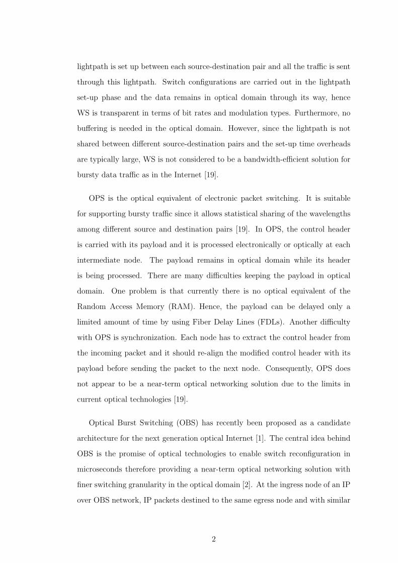

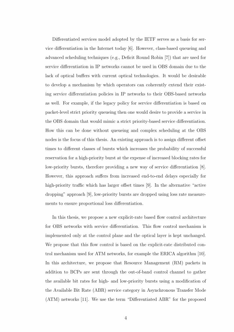
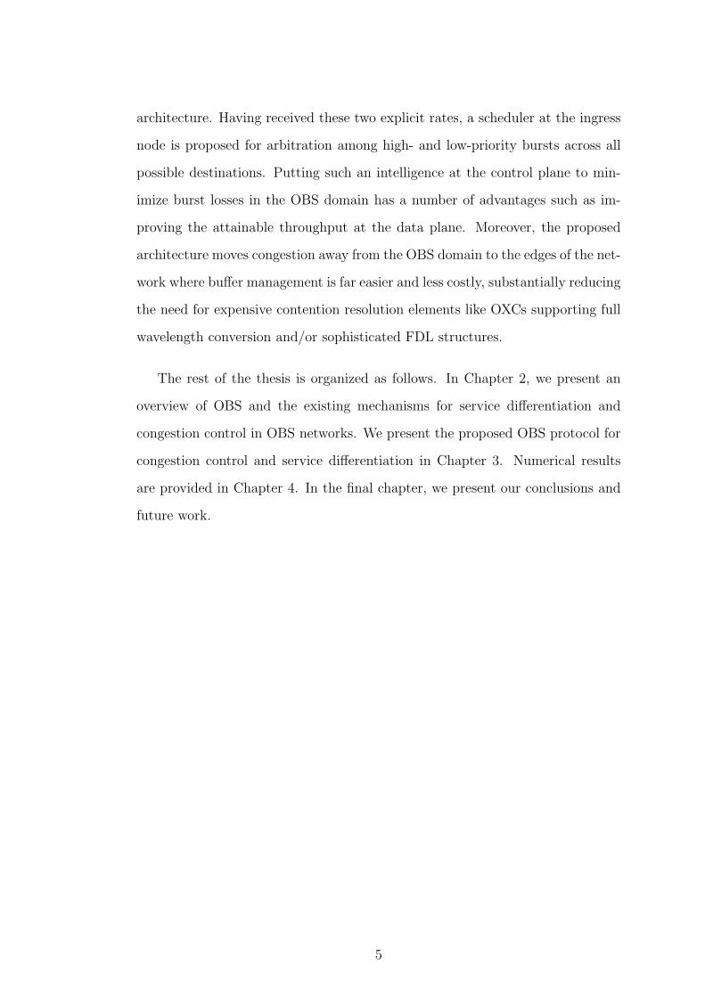
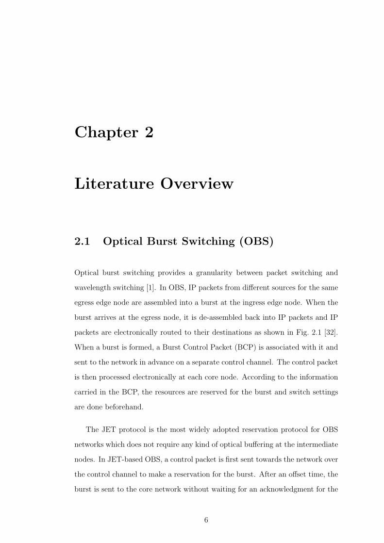
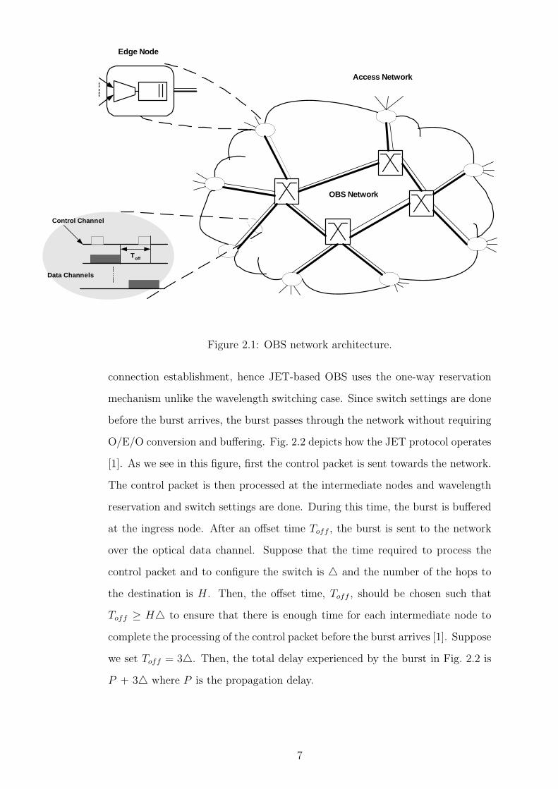
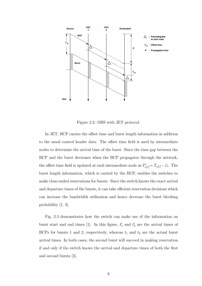


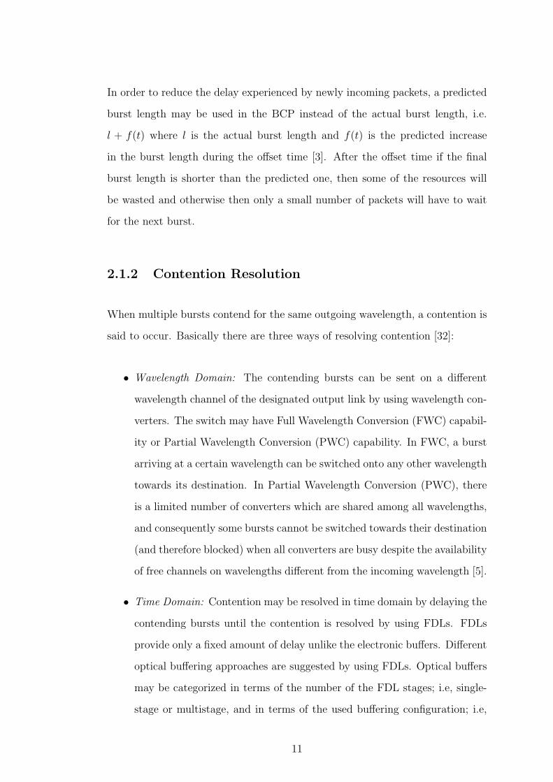

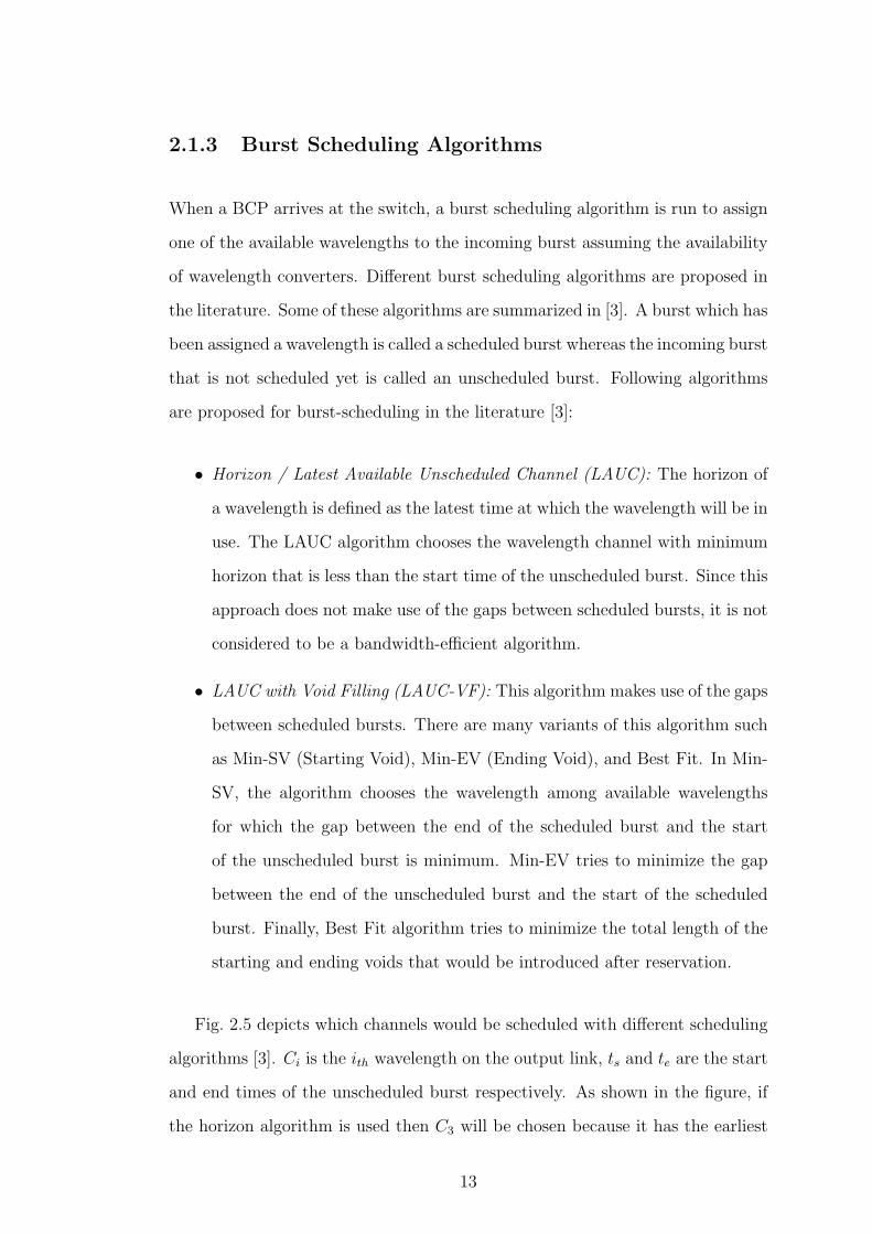
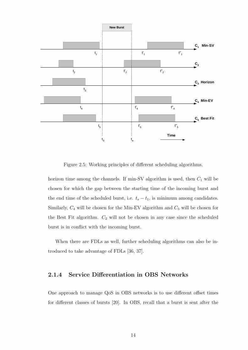

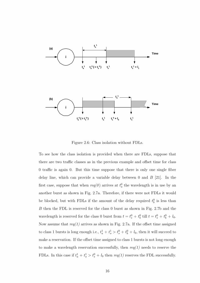
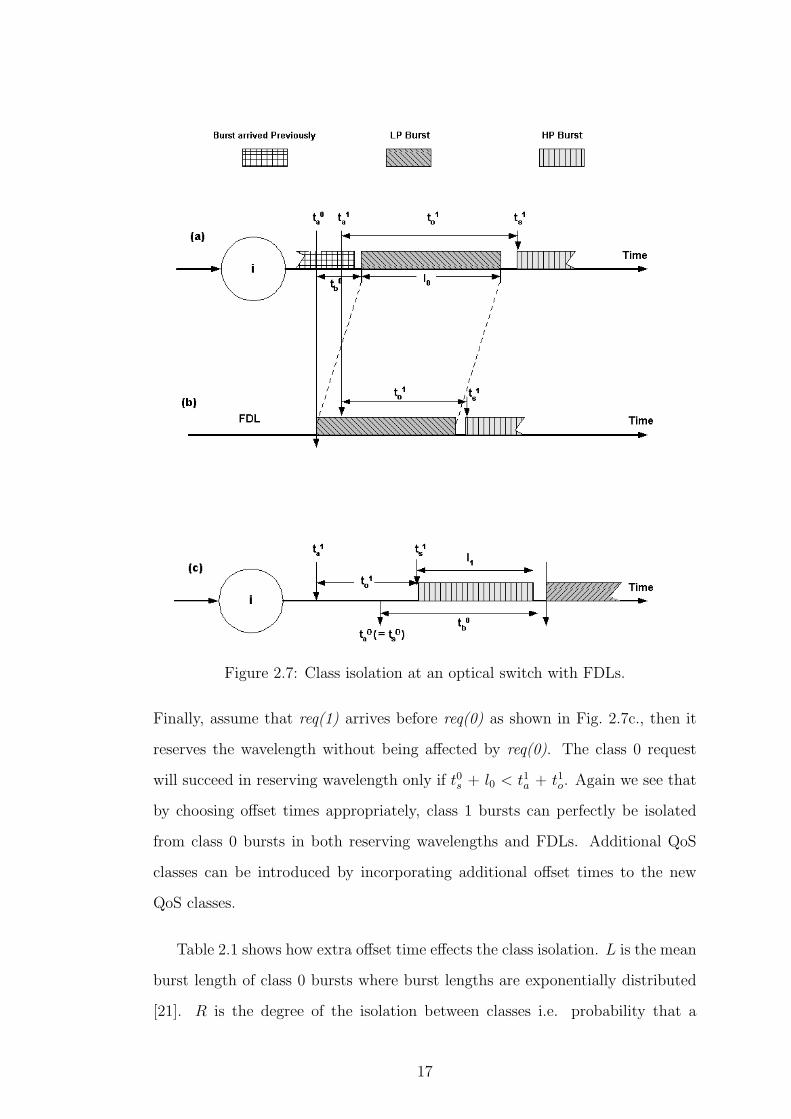
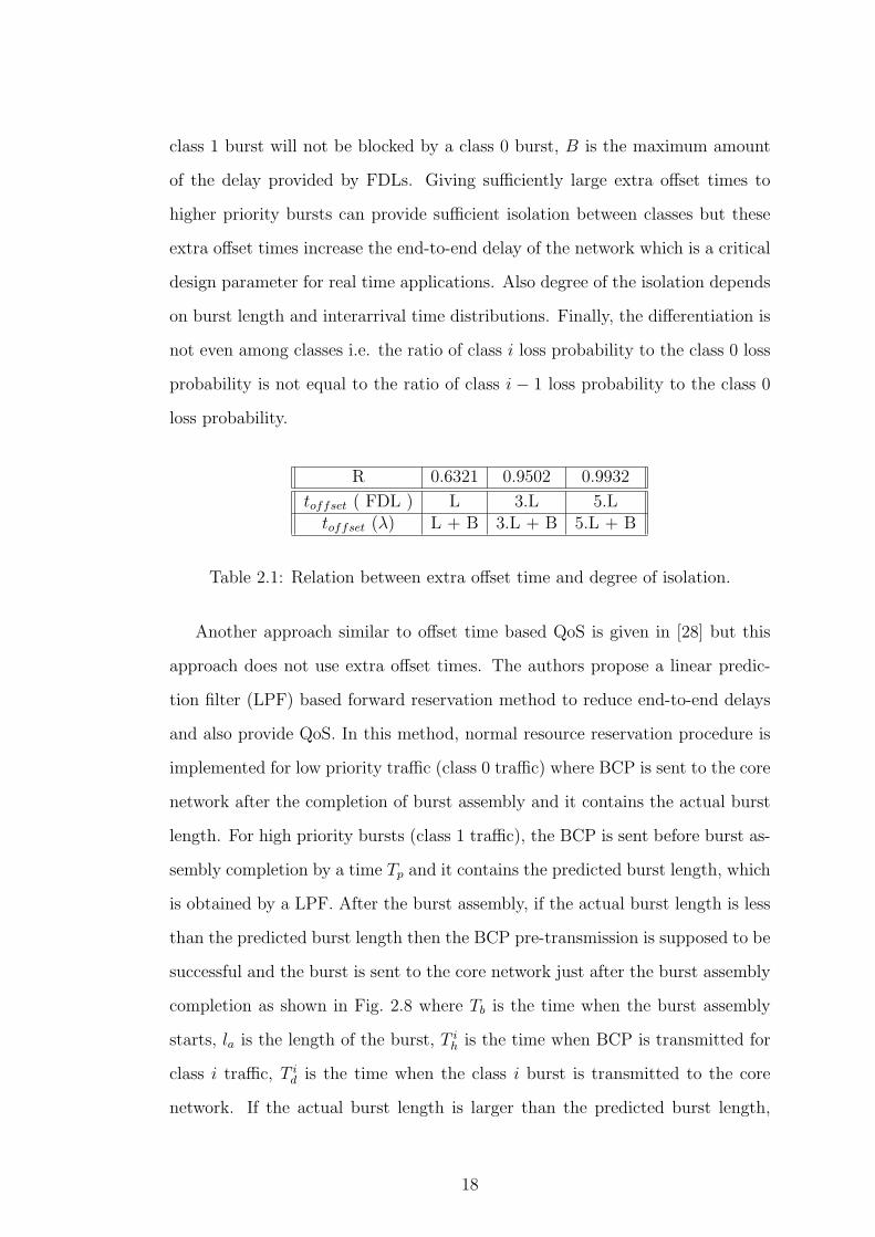
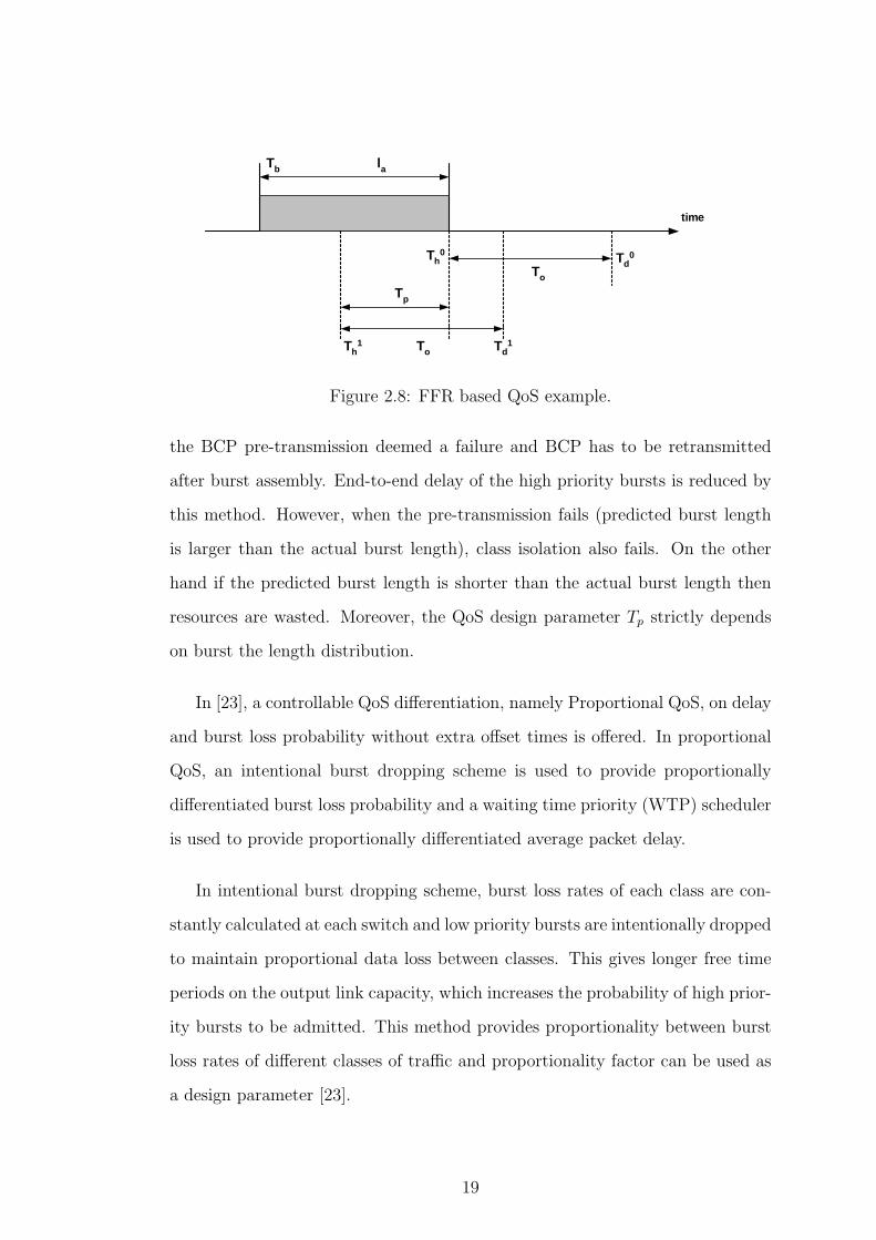


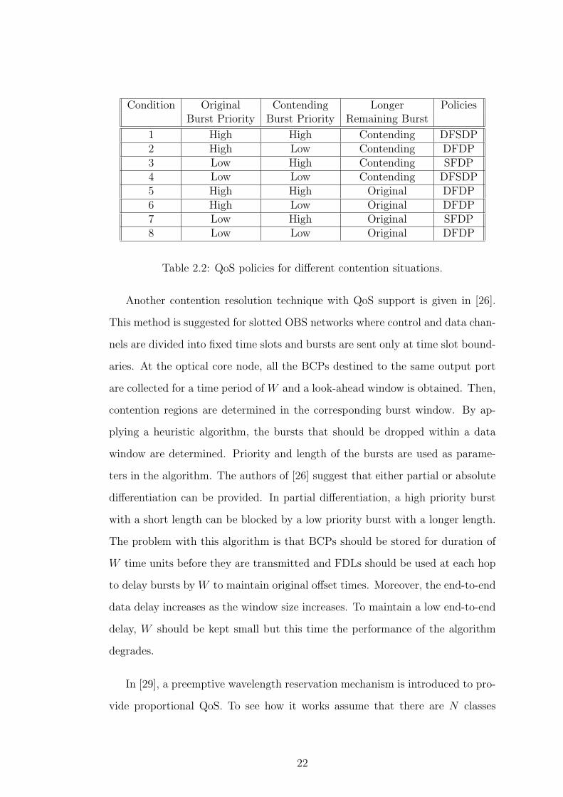


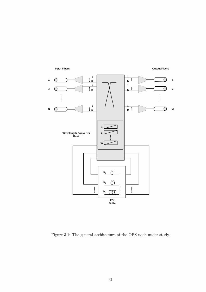

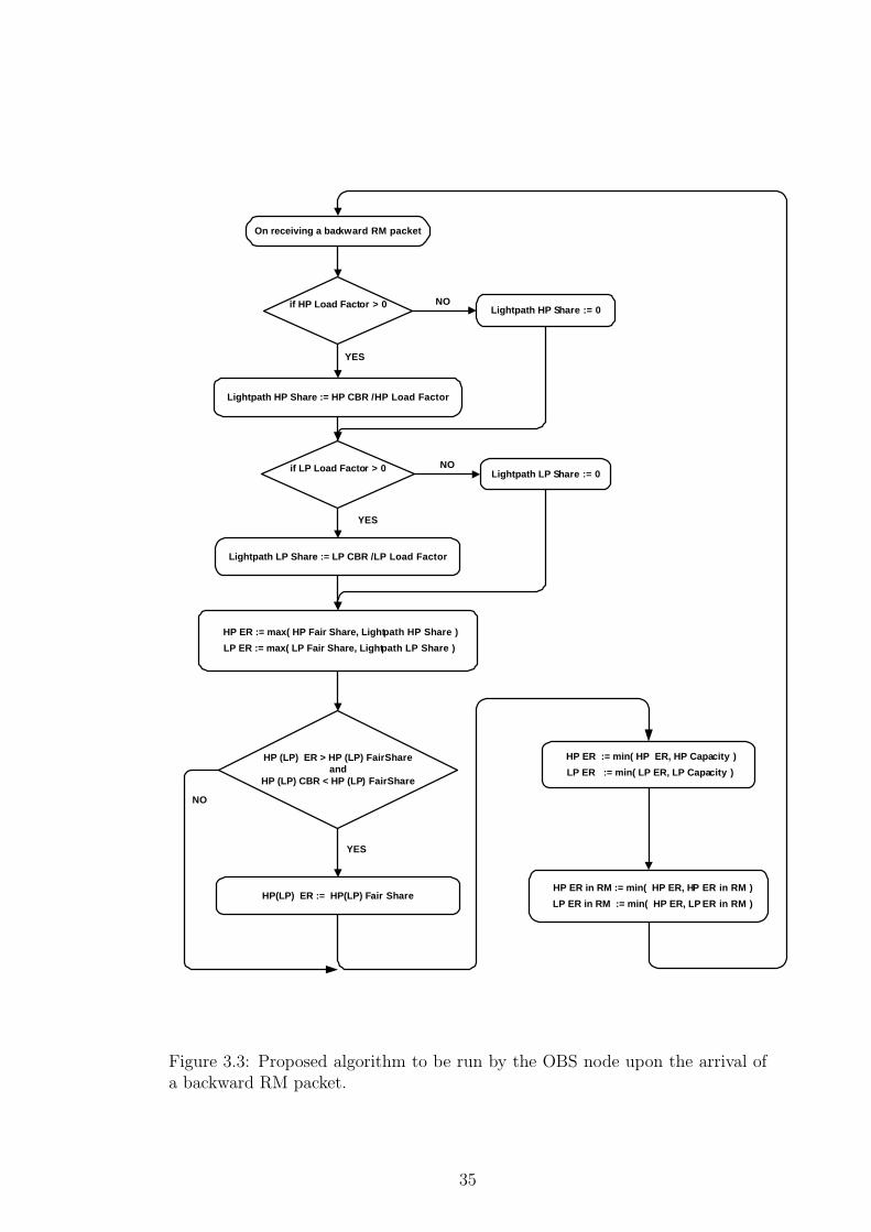

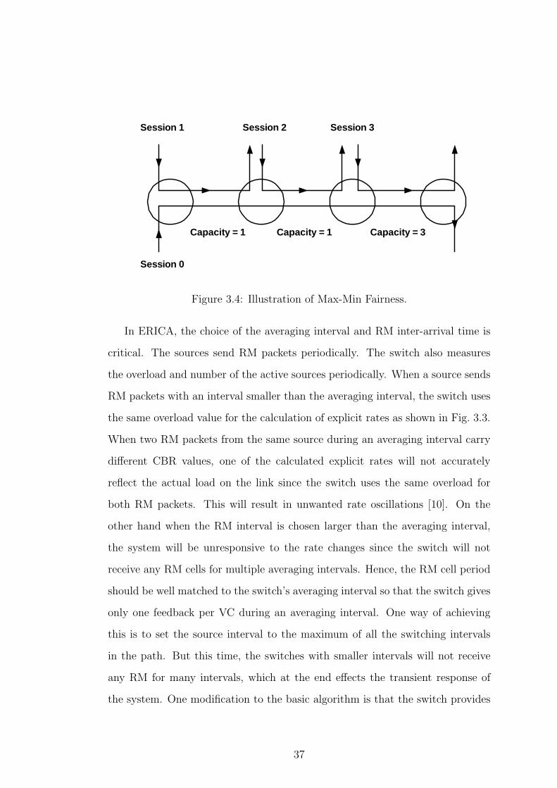


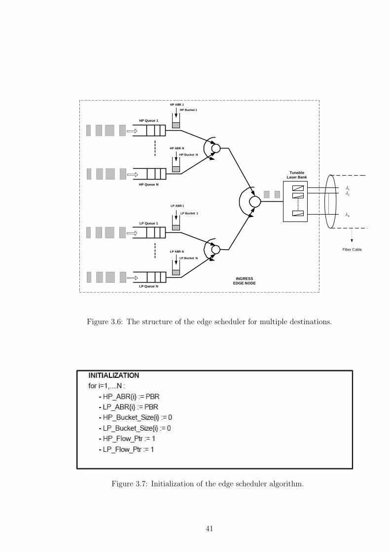
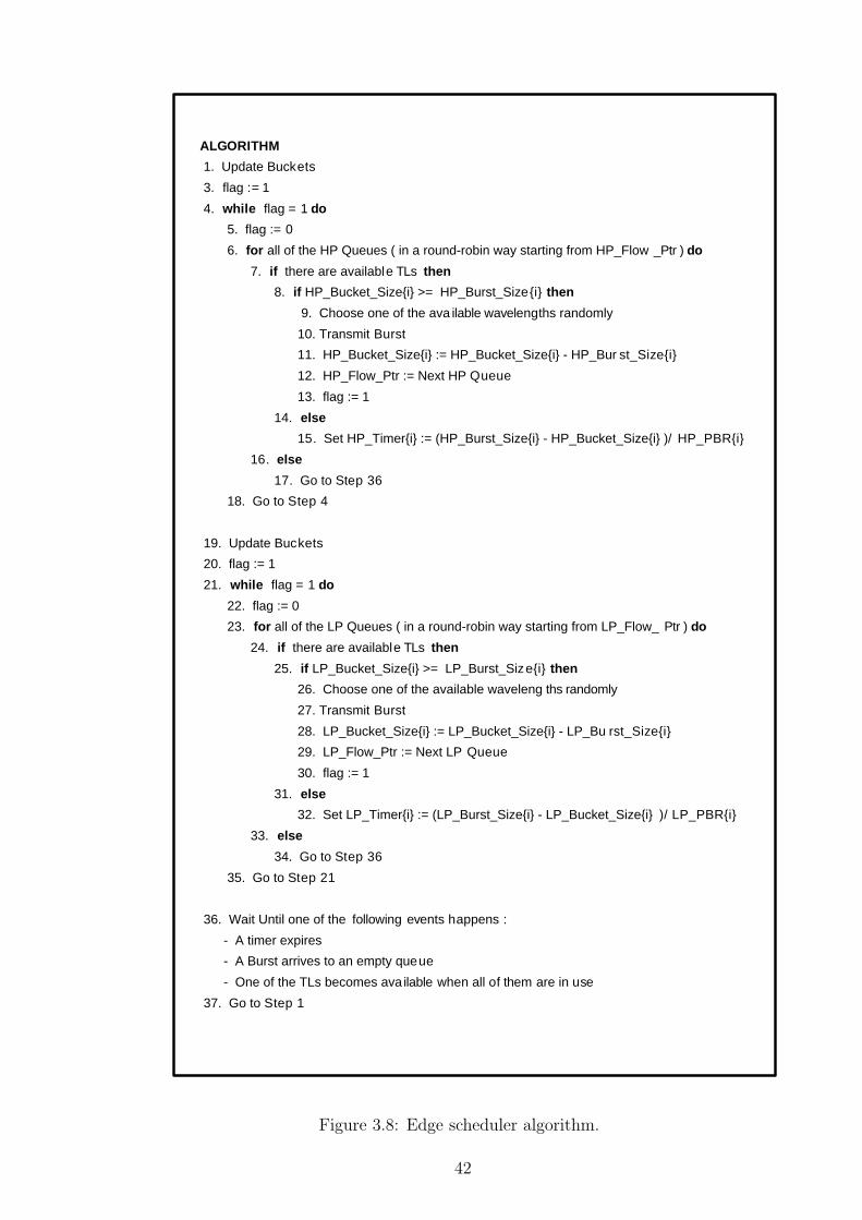

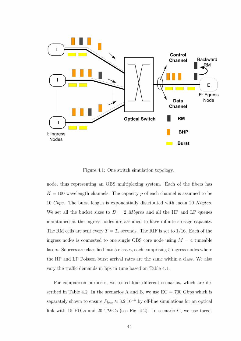


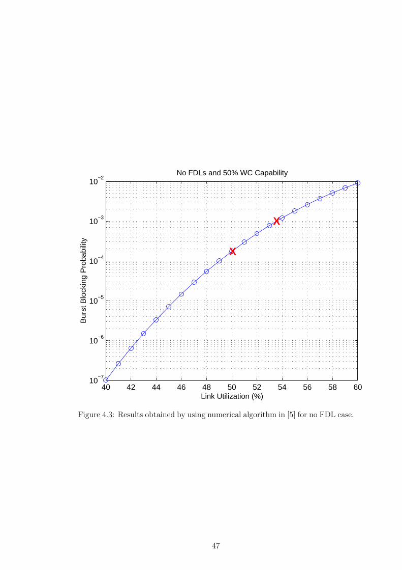
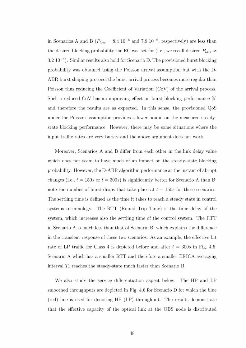
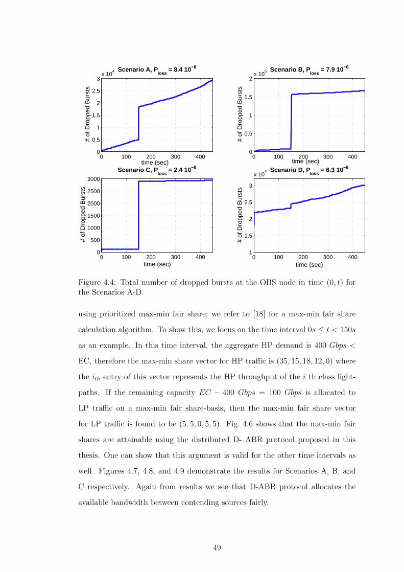

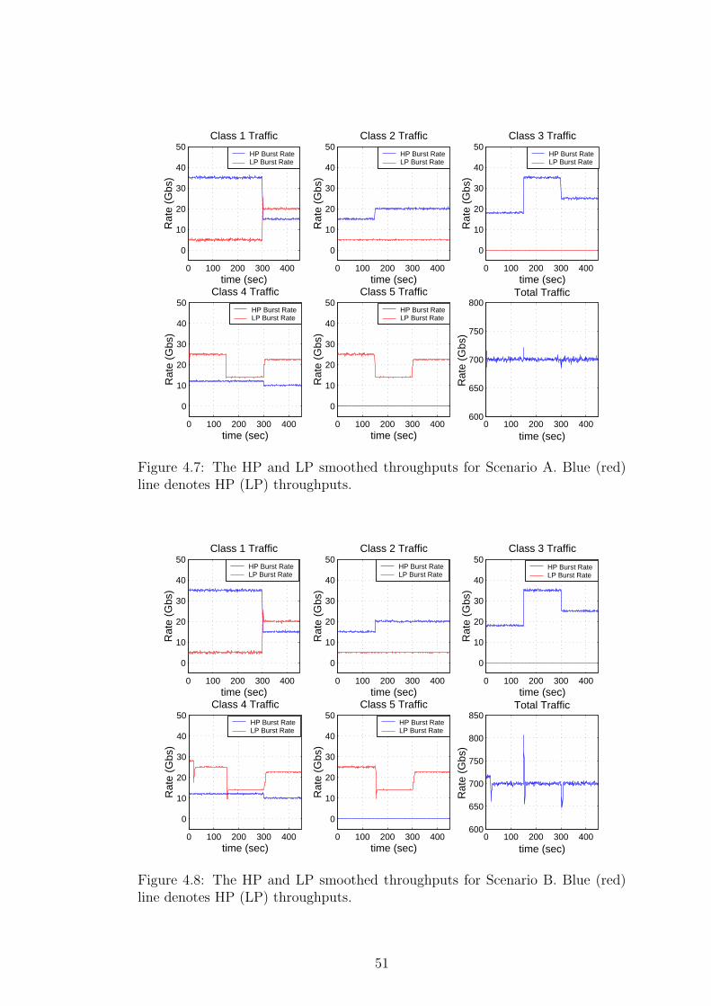
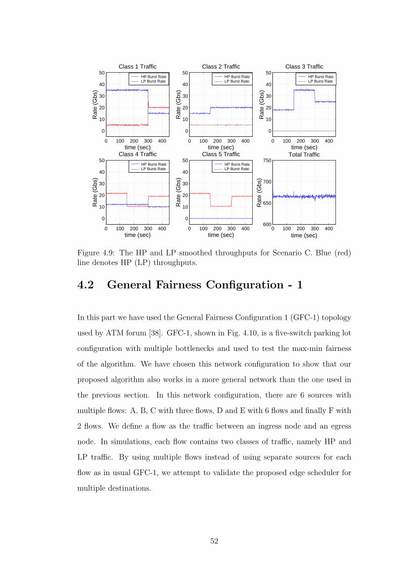
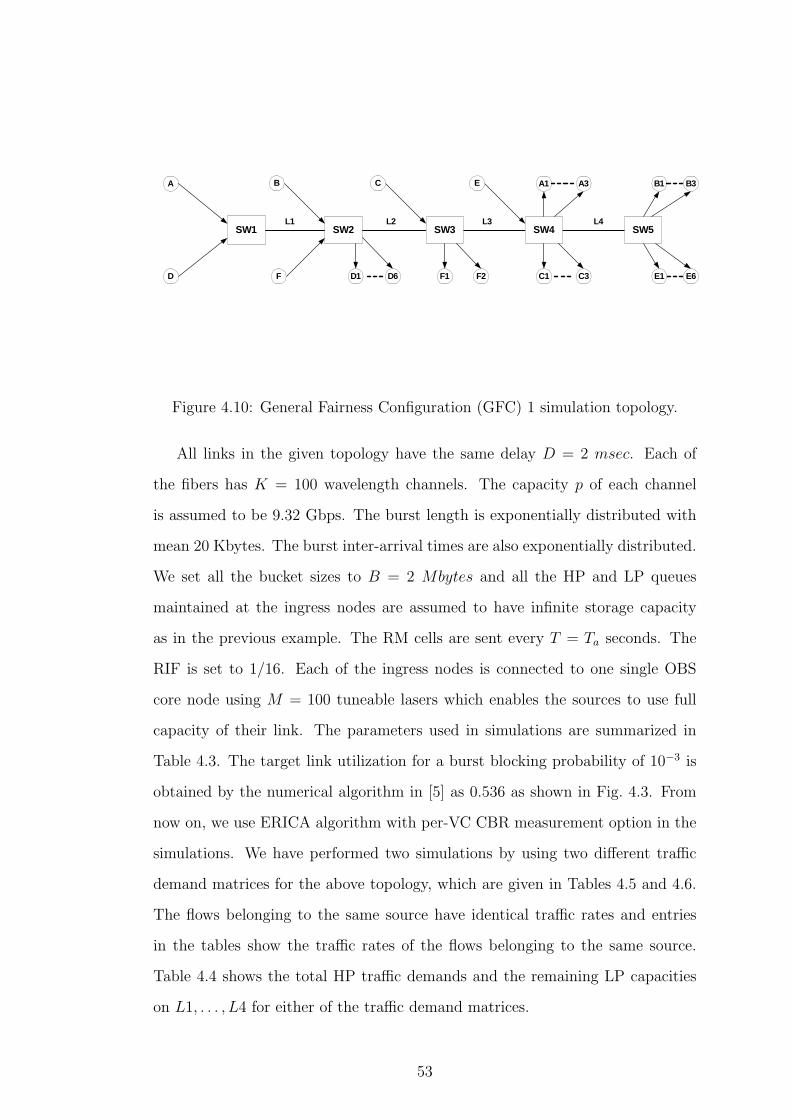


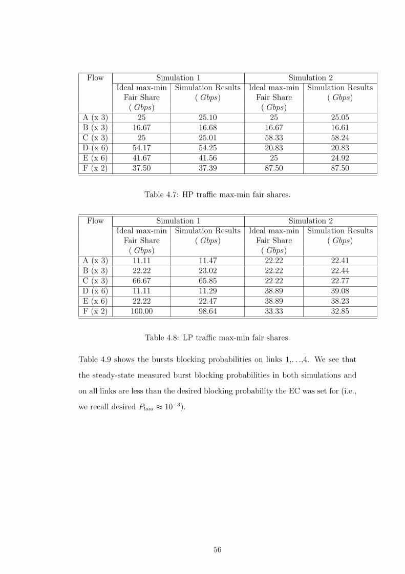
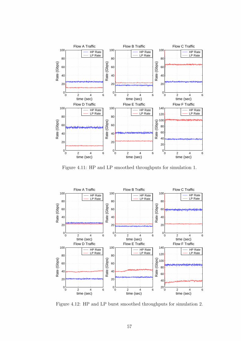


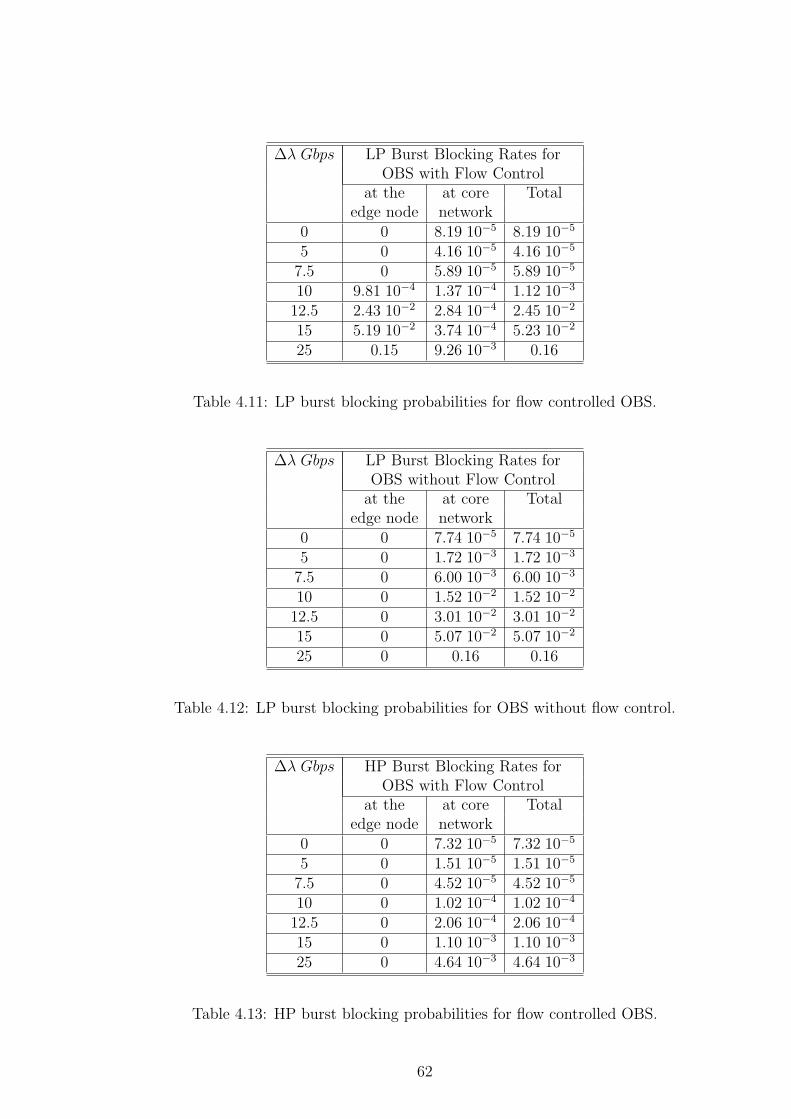

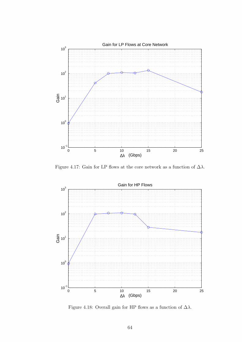

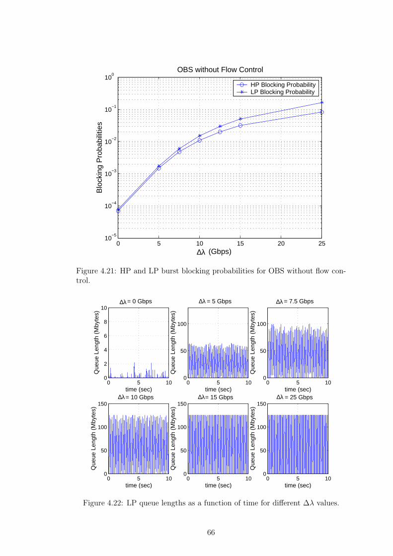
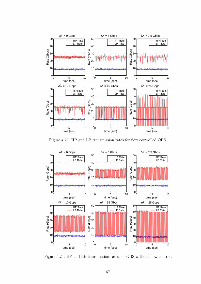
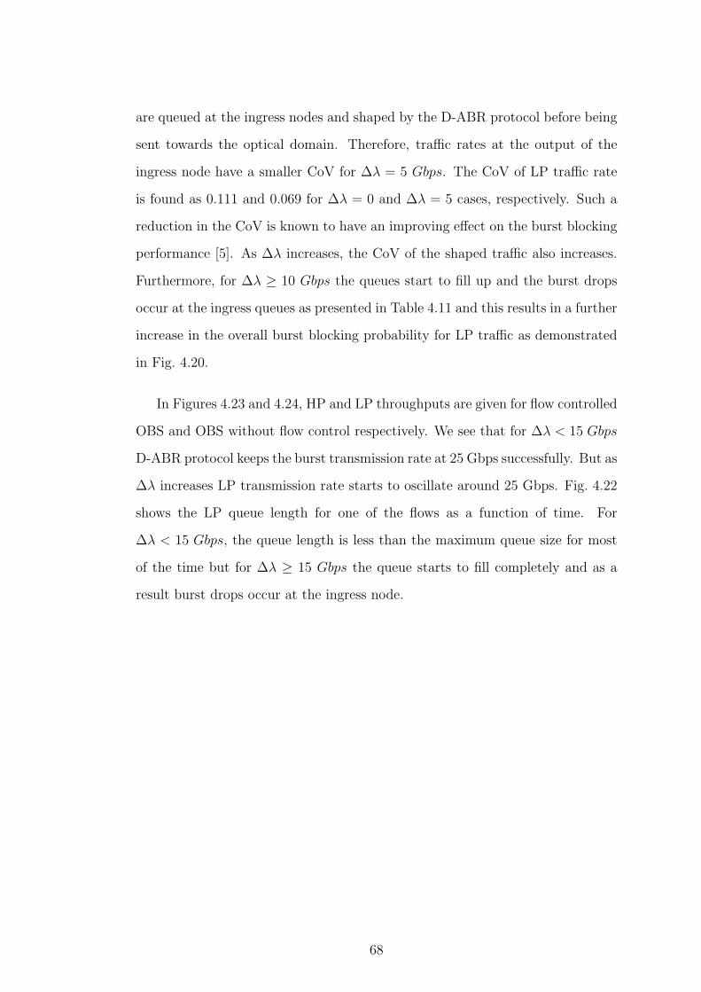


![Traffic analysis in optical burst switching networks: a trace-based … · 2009-11-10 · TRAFFIC ANALYSIS IN OPTICAL BURST SWITCHING NETWORKS In Reference [11] a trace-based simulation](https://static.documents.pub/doc/80x56/5e9136798bc3a102d27c27ce/traffic-analysis-in-optical-burst-switching-networks-a-trace-based-2009-11-10.jpg)