CHE 2161

Fluid Mechanics

Lab Report – Flow Measurements

1.0 Abstract

In the given experiment, the Bernoulli equation was tested along with the mass continuity principle. In

order to successfully show how well the two principles hold within the limits of this experiment, the

volumetric flow rate had to be calculated; and the ratio of actual flow rate to ideal flow rate, otherwise

known as the discharge coefficient, had to be verified. Upon comparison however, it was observed that

Bernoulli’s equation cannot be used to determine the flow rate accurately, as the processed data for the

Reynolds number and discharge coefficient did not fall within the specified literature value data range.

This deviation could be due to errors that accumulated during the experiment. Some of the common

errors may have included human error when timing and parallax error when taking readings, causing

the fluctuations in the results; also energy losses and frictional losses within the system, and changes

in fluid properties.

2.0 Introduction

There are various methods of measuring volumetric the flow rate flow rate. In this experiment, four

instrumental methods are carried out Didacta Italia Rig. The four methods are orifice plate, turbine flow

meter, venture tube and rotameter.

The theories behind the flow meters are conservation of mass and the Bernoulli equation. From

conservation of mass, we understand that the reduction of cross sectional area will cause an increase

of velocity. From the Bernoulli equation, we know this will lead to an increase in pressure. The Bernoulli

equation is 21constant

2V P gz .

2.1 Description of flow measurement techniques:

1. Orifice plate

In this method, there is a sudden decrease in the cross sectional area of the pipe. This causes

increase in the velocity of the fluid, thereafter causing decrease in pressure, as described in the

theories above. The orifice plate is accurate and the cost of the instrument is low when compared

to other instruments. However, this method can only work with homogenous liquids and under

axial velocity vector flow.

2. Turbine Flow Meter

The turbine flow meter uses a bladed rotor suspended in the pipe. As the fluid flows through the

pipe, the rotor spins at a rate proportional to the fluids velocity. One limitation of turbine flow

meters is the fact that can only operate with clean, low-viscosity, non- corrosive fluids. The

upside is that turbine meters can operate in a wide range of temperatures and pressures.

3. Venturi Tube

The venture tube has a gradual contraction, followed by a gradual expansion. The principle used

is the same as an orifice plate. One drawback of using a venture meter to measure flow rate is

that they are heavy and maintenance is not easy. However, they do allow larger pressure drops.

4. Rotameter

The rotameter consists of a tube and a float. The float response to flow rate is linear. An

advantage of the rotameter is it does not require any external power or fuel. This is because it

uses the properties of fluid along with gravity to measure flow rate. A disadvantage of using a

rotameter is that since it uses gravity, it must always be vertical and the right way up.

2.2 Practical applications

1. Airplanes have a pitot tube attached to them to measure the speed of the aircraft

2. Race cars such as Formula 1 cars use the theory of Bernoulli’s equation to allow the car to be on

the ground at very high speeds.

3. Carburetors found in cars and other motorized machines have a venturi meter to maintain low

pressure so as to let fuel in.

4. Venturi meters are used in plumbing as well. They are used in wastewater collection systems

and treatment plants because their design allow solids to pass through.

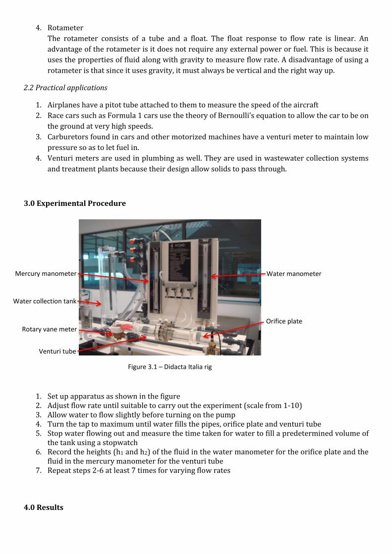
3.0 Experimental Procedure

1. Set up apparatus as shown in the figure 2. Adjust flow rate until suitable to carry out the experiment (scale from 1-10) 3. Allow water to flow slightly before turning on the pump 4. Turn the tap to maximum until water fills the pipes, orifice plate and venturi tube 5. Stop water flowing out and measure the time taken for water to fill a predetermined volume of

the tank using a stopwatch 6. Record the heights (h1 and h2) of the fluid in the water manometer for the orifice plate and the

fluid in the mercury manometer for the venturi tube 7. Repeat steps 2-6 at least 7 times for varying flow rates

4.0 Results

Mercury manometer Water manometer

Orifice plate

Venturi tube

Water collection tank

Rotary vane meter

Figure 3.1 – Didacta Italia rig

Figure 4.1: Graph of the Discharge Coefficient

vs The Reynolds Number for the Orifice Plate

Using continuity: m1̇ = m2̇ ρ1A1v1 = ρ2A2v2 Assumption: Incompressible fluid flow (ρ1 = ρ2)

π

4D2v1 =

π

4d2v2

𝐯𝟐 = 𝐃𝟐

𝐝𝟐 𝐯𝟏 ................................................................... (1)

Using Bernoulli equation: Assumption: Steady, incompressible fluid flow, inviscid flow (no viscosity), with no work done by or on the fluid.

P1 +1

2ρv1

2 + ρgh1 = P2 +1

2ρv2

2 + ρgh2 (h1 ≈ h2)

P1 +1

2ρv1

2 = P2 +1

2ρv2

2

𝐏𝟏 − 𝐏𝟐 = 𝟏

𝟐𝛒𝐰[𝐯𝟐

𝟐 − 𝐯𝟏𝟐] ................................................................. (2)

Substitute [1] in [2]

[(𝐃𝟐

𝐝𝟐)

2

− 1] v12 =

2(P1−P2)

ρw

𝐯𝟏 = √𝟐(𝐏𝟏−𝐏𝟐)

𝛒𝐰((𝐃

𝐝)

𝟒−𝟏)

Therefore, 𝐐𝐈𝐝𝐞𝐚𝐥 = 𝐯𝟏𝐀𝟏 = 𝛑𝐃𝟐

𝟒 √𝟐(𝐏𝟏−𝐏𝟐)

𝛒𝐰((𝐃

𝐝)

𝟒−𝟏)

................................................................. (3)

To determine the QActual 6L of water was collected in a time period. 𝐐𝐀𝐜𝐭𝐮𝐚𝐥 = 𝐕𝐨𝐥𝐮𝐦𝐞 𝐜𝐨𝐥𝐥𝐞𝐜𝐭𝐞𝐝

𝐭𝐢𝐦𝐞

Discharge coefficient, 𝐂𝐝 = 𝐐 𝐀𝐜𝐭𝐮𝐚𝐥

𝐐 𝐈𝐝𝐞𝐚𝐥

Calculations for Orifice plate Calculation for Venturi tube (P1 − P2) = (ρwater − ρair)x g x |∆h|

ρair = 1.23 kg/m3 ρwater = 998kg/m3

D = 50mm , d = 20mm v1,orifice = QIdeal/A1

Re = (v1,orifice × ρwater × D)/μwater

(P1 − P2) = (ρmercury − ρwater)x g x |∆h|

ρmercury = 13000kg/m3

ρwater = 998kg/m3 v1,venturi = QIdeal/A1

D = 20mm , d = 10mm Re = (v1,venturi × ρwater × D)/μwater

0.48

0.5

0.52

0.54

0.56

0.58

0.6

0.62

0.64

0.66

0 5000 10000 15000

Dis

char

ged

Co

eff

icie

nt

,Cd

Reynolds Number ,Re

Orifice Plate

Figure 4.2: Graph of the Discharge Coefficient

vs The Reynolds Number for the Venturi Tube

Figure 4.3: Graph of the Rotameter versus the actual flow 5.0 Discussion 5.0.1 Comparison of Processed Data to Literature Values During the experiment it was noted that the ratio of the diameter of the throat to that of the upstream was 0.4. Also as per table A3, given in the appendices of this report, the results for the orifice plate can be summarized as data ranges of 2366 to 10412 for the Reynolds number, and 0.49 to 0.64 for the discharge coefficient. We noted down the literature value from a graph taken from Munson’s Fundamentals of Fluid Mechanics plotting the Discharge Coefficient vs. Reynolds Number for an Orifice Plate, and we noted that for a ratio of the throat diameter to the upstream of 0.4, the Reynolds number ranged from 104 to 105 and the discharge coefficient ranged from 0.60 to 0.61. Upon comparison between the literature value and the results we noticed that the processed data range of 0.49<Re < 0.60 and 0.61<Re < 0.64 for the discharged coefficient, and the values for the Reynolds number do not corroborate the expected results and this can be attributed to experimental errors which will be discussed in detail in the latter part of this discussion.

0.68

0.7

0.72

0.74

0.76

0.78

0.8

0.82

0.84

0.86

0 5000 10000 15000 20000 25000 30000

Dis

char

ged

Co

eff

icie

nt

,Cd

Reynolds Number ,Re

Venturi Tube

0

0.05

0.1

0.15

0.2

0.25

0.3

0.35

0.4

0.45

0 0.05 0.1 0.15 0.2 0.25 0.3 0.35 0.4 0.45

Ro

tam

ete

r R

ead

ing

(×10

-3m

3/s

)

Actual flow ((×10-3 m3/s)

Rotameter reading vs Actual flowrate

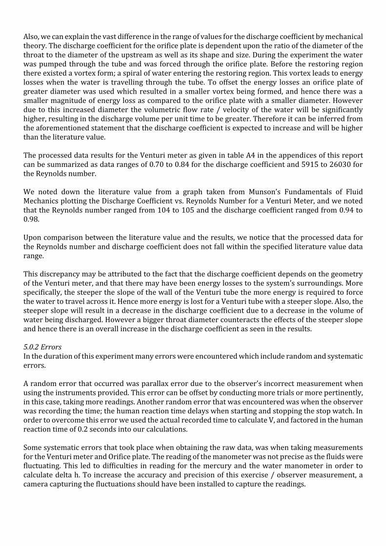
Also, we can explain the vast difference in the range of values for the discharge coefficient by mechanical theory. The discharge coefficient for the orifice plate is dependent upon the ratio of the diameter of the throat to the diameter of the upstream as well as its shape and size. During the experiment the water was pumped through the tube and was forced through the orifice plate. Before the restoring region there existed a vortex form; a spiral of water entering the restoring region. This vortex leads to energy losses when the water is travelling through the tube. To offset the energy losses an orifice plate of greater diameter was used which resulted in a smaller vortex being formed, and hence there was a smaller magnitude of energy loss as compared to the orifice plate with a smaller diameter. However due to this increased diameter the volumetric flow rate / velocity of the water will be significantly higher, resulting in the discharge volume per unit time to be greater. Therefore it can be inferred from the aforementioned statement that the discharge coefficient is expected to increase and will be higher than the literature value. The processed data results for the Venturi meter as given in table A4 in the appendices of this report can be summarized as data ranges of 0.70 to 0.84 for the discharge coefficient and 5915 to 26030 for the Reynolds number. We noted down the literature value from a graph taken from Munson’s Fundamentals of Fluid Mechanics plotting the Discharge Coefficient vs. Reynolds Number for a Venturi Meter, and we noted that the Reynolds number ranged from 104 to 105 and the discharge coefficient ranged from 0.94 to 0.98. Upon comparison between the literature value and the results, we notice that the processed data for the Reynolds number and discharge coefficient does not fall within the specified literature value data range. This discrepancy may be attributed to the fact that the discharge coefficient depends on the geometry of the Venturi meter, and that there may have been energy losses to the system’s surroundings. More specifically, the steeper the slope of the wall of the Venturi tube the more energy is required to force the water to travel across it. Hence more energy is lost for a Venturi tube with a steeper slope. Also, the steeper slope will result in a decrease in the discharge coefficient due to a decrease in the volume of water being discharged. However a bigger throat diameter counteracts the effects of the steeper slope and hence there is an overall increase in the discharge coefficient as seen in the results. 5.0.2 Errors In the duration of this experiment many errors were encountered which include random and systematic errors. A random error that occurred was parallax error due to the observer’s incorrect measurement when using the instruments provided. This error can be offset by conducting more trials or more pertinently, in this case, taking more readings. Another random error that was encountered was when the observer was recording the time; the human reaction time delays when starting and stopping the stop watch. In order to overcome this error we used the actual recorded time to calculate V, and factored in the human reaction time of 0.2 seconds into our calculations. Some systematic errors that took place when obtaining the raw data, was when taking measurements for the Venturi meter and Orifice plate. The reading of the manometer was not precise as the fluids were fluctuating. This led to difficulties in reading for the mercury and the water manometer in order to calculate delta h. To increase the accuracy and precision of this exercise / observer measurement, a camera capturing the fluctuations should have been installed to capture the readings.

6.0 Conclusion In the duration of this experiment, various instruments were used to collect raw data and process this data to calculate the volumetric flow rates. However, the data that which was collected from each instrument yielded different results as compared to the expected flow rate (Bernoulli’s Principle was employed to calculate the value of the ideal volumetric flow rate), which can be owed to uncertainties that arose due to experimental errors. 7.0 Refereces

1. Munson, Young, Okiishi 2007, Fundamentals of Fluid Mechanics, 5th Edition. pp. 513-516

2. http://www.kellyaerospace.com/articles/Accessory_AMT.pdf [Accessed: 13.09. 2013]

3. http://www.engineeringtoolbox.com/pitot-tubes-d_612. [Accessed: 13.09. 2013]

4. http://www.scienceclarified.com/everyday/Real-Life-Chemistry-Vol-3-Physics-Vol-

1/Bernoulli-s-Principle-Real-life-applications.html#b [Accessed: 13.09. 2013]

Appendices

Appendix I: Raw Data

Table A1: Set of values measured during the experiment

No Scale Measurement

(Actual Flow Rate) Orifice Plate, Water Manometer D=50mm, d=20mm

Venturi Tube, Mercury Manometer

Rotameter (m3/h)

Volume (L) Time (s)

h1(cm) h2(cm) h1(cm) h2(cm)

1 6.0 14.6 29.5 8.7 7.4 22.2 1.5 2 6.0 14.56 29.1 8.6 7.4 22.2 1.5 3 6.0 15.63 26.3 8.6 8.5 21 1.4 4 6.0 18.46 21 8 10.2 19.3 1.2 5 6.0 22.37 15.4 6.7 11.5 17.9 0.9 6 6.0 27.59 10.7 5 12.7 16.9 0.8 7 6.0 36.59 6 2.6 13.6 16 0.6 8 6.0 64.25 1.8 0 14.3 15.4 0.3

Appendix II: Calculated Values

Table A2: Results of the volumetric flow rate for the Rotameter and the actual flow rate.

Rotameter Qactual

Qrotameter

(m3/h) (m3/s) (x10-3) (m3/s) (x10-3)

1.5 0.416666667 0.402

1.5 0.416666667 0.379

1.4 0.388888889 0.344

1.2 0.333333333 0.318

0.9 0.25 0.297

0.8 0.222222222 0.281

0.6 0.166666667 0.252

0.3 0.083333333 0.219

Table A3: Values Calculated for the Orifice Plate

Table A4: Values Calculated for the Venturi Meter

Orifice Plate, Water Manometer

h1

(m) h2 (m) Δh (m) ΔP (Pa)

Vorifice

(m/s)

Qideal

x10-3 (m3/s)

Reynolds

Number, Re

Discharge

Coefficient, CD

0.295 0.087 0.208 2033.889 0.2092996 0.0006425 10412.814 0.639593047

0.291 0.086 0.205 2004.554 0.2098746 0.0006379 10441.42063 0.646025933

0.263 0.086 0.177 1730.762 0.1955070 0.0005927 9726.620881 0.647653395

0.21 0.08 0.13 1271.181 0.1655349 0.00050797 8235.486694 0.639859886

0.154 0.067 0.087 850.7133 0.1366015 0.00041555 6796.025229 0.645450062

0.107 0.05 0.057 557.3639 0.1107566 0.00033636 5510.224153 0.646545553

0.06 0.026 0.034 332.4627 0.0835139 0.00025978 4154.880688 0.631228195

0.018 0 0.018 176.0096 0.0475607 0.00018901 2366.180302 0.494059066

Venturi Meter, Mercury Manometer

h1 (m) h2 (m) Δh (m) ΔP (Pa) Vorifice

(m/s)

Qideal

x10-3 (m3/s)

Reynolds

Number,

Re

Discharge

Coefficient, CD

0.074 0.222 0.148 18296.59 1.3081228 0.0004912 26032.035 0.8366798

0.074 0.222 0.148 18296.59 1.3117165 0.0004912 26103.552 0.83897836

0.085 0.21 0.125 15453.2 1.2219189 0.0004514 24316.552 0.85041127

0.102 0.193 0.091 11249.93 1.0345933 0.0003851 20588.717 0.84389924

0.115 0.179 0.064 7912.04 0.8537592 0.0003230 16990.063 0.83039939

0.127 0.169 0.042 5192.276 0.6922288 0.0002617 13775.560 0.83112557

0.136 0.16 0.024 2967.015 0.5219620 0.0001978 10387.202 0.82903899

0.143 0.154 0.011 1359.882 0.2972543 0.0001340 5915.4508 0.69738647

Appendix III: Sample calculation for Orifice plate (D=50mm, d=20mm) Reading 1: H1=29.5mm H2=8.7mm Volume=6L Time=14.6s Referring to the table (P1 − P2) = (ρwater − ρair)x g x |∆h| (P1 − P2) = (998 − 1.23)x 9.81 x |0.208m| = 2033.889𝑃𝑎 By using the equation 3

QIdeal = v1A1 = πD2

4 √2(P1−P2)

ρw((D

d)

4−1)

QIdeal = v1A1 = π0.052

4 √2(2033.889)

998((0.05

0.02)

4−1)

= 0.0006425 m3 s⁄

QActual = Volume collected

time=

0.006m3

14.6= 0.0004109 m3 s⁄

Discharge coefficient, Cd = Q Actual

Q Ideal=

0.0004109

0.0006425= 0.6396

vOrifice =QIdeal

A1=

0.0006425

0.001964= 0.2093m/s

Re =v1,orifice×ρwater×D

μwater=

0.2093×998×0.05

0.001003= 10412.6

Appendix IV: Imported Graphs

Figure A5: Graph of the Discharge Coefficient

vs Reynolds number for the venturi meter

Figure A6: Graph of the Discharge Coefficient

vs Reynolds number for the Orifice