Page 1
FLOW OF A NON-NEWTONIAN BINGHAM PLASTIC
FLUID OVER A ROTATING DISK
A Thesis
Submitted to the College of Graduate Studies and Research
In Partial Fulfillment of the Requirements
For the Degree of
Doctor of Philosophy
in the Department of Mechanical Engineering
University of Saskatchewan
Saskatoon, Saskatchewan
By
Ali A. Rashaida
Copyright Ali A. Rashaida, August 2005. All rights reserved.
Page 2
PERMISSION TO USE
The author has agreed that the library, University of Saskatchewan, may make
this thesis freely available for inspection. Moreover, the author has agreed that
permission for extensive copying of this thesis for scholarly purposes may be granted by
the professors who supervised the thesis work recorded herein or, in their absence, by the
Head of the Department or Dean of the College in which the thesis work was done. It is
understood that due recognition will be given to the author of this thesis, supervisors and
to the University of Saskatchewan in any use of the material in this thesis. Copying or
publication or any other use of this thesis for financial gain without the approval by the
University of Saskatchewan and the author’s written permission is prohibited.
Requests for permission to copy or to make any other use of material in this thesis
in whole or in part should be addressed to:
Head of the Department of Mechanical Engineering,
57 Campus Drive,
University of Saskatchewan,
Saskatoon, Saskatchewan, Canada.
S7N 5A9
i
Page 3
ABSTRACT
Even though fluid mechanics is well developed as a science, there are many
physical phenomena that we do not yet fully understand. One of these is the deformation
rates and fluid stresses generated in a boundary layer for a non-Newtonian fluid. One
such non-Newtonian fluid would be a waxy crude oil flowing in a centrifugal pump. This
type of flow can be numerically modeled by a rotating disk system, in combination with
an appropriate constitutive equation, such as the relation for a Bingham fluid. A Bingham
fluid does not begin to flow until the stress magnitude exceeds the yield stress. However,
experimental measurements are also required to serve as a database against which the
results of the numerical simulation can be interpreted and validated.
The purpose of the present research is to gain a better understanding of the
behavior of a Bingham fluid in the laminar boundary layer on a rotating disk. For this
project, two different techniques were employed: numerical simulation, and laboratory
investigations using Particle Image Velocimetry (PIV) and flow visualization. Both
methods were applied to the flow of a Bingham fluid over a rotating disk.
In the numerical investigations, the flow was characterized by the dimensionless
yield stress “Bingham number”, By, which is the ratio of the yield and viscous stresses.
Using von Kármán’s similarity transformation, and introducing the rheological behavior
of the fluid into the conservation equations, the corresponding nonlinear two-point
boundary value problem was formulated. A solution to the problem under investigation
ii
Page 4
was obtained by numerical integration of the set of Ordinary Differential Equations
(ODEs) using a multiple shooting method. The influence of the Bingham number on the
flow behavior was identified. It decreases the magnitude of the radial and axial velocity
components, and increases the magnitude of the tangential velocity component, which
has a pronounced effect on the moment coefficient, CM, and the volume flow rate, Q.
In the laboratory investigations, since the waxy crude oils are naturally opaque, an
ambitious experimental plan to create a transparent oil that was rheologically similar to
the Amna waxy crude oil from Libya was developed. The simulant was used for flow
visualization experiments, where a transparent fluid was required. To fulfill the demand
of the PIV system for a higher degree of visibility, a second Bingham fluid was created
and rheologically investigated. The PIV measurements were carried out for both filtered
tap water and the Bingham fluid in the same rotating disk apparatus that was used for the
flow visualization experiments. Both the axial and radial velocity components in the (r-z)
plane were measured for various rotational speeds.
Comparison between the numerical and experimental results for the axial and
radial velocity profiles for water was found to be satisfactory. Significant discrepancies
were found between numerical results and measured values for the Bingham fluid,
especially at low rotational speeds, mostly relating to the formation of a yield surface
within the tank.
iii
Page 5
Even though the flow in a pump is in some ways different from that of a disk
rotating in a tank, some insight about the behavior of the pump flow can be drawn. One
conclusion is that the key difference between the flow of a Bingham fluid in rotating
equipment from that of a Newtonian fluid such as water relates to the yield surface
introduced by the yield stress of the material, which causes an adverse effect on the
performance and efficiency of such equipment.
iv
Page 6
ACKNOWLEDGEMENT
I would like to express my profound appreciation and sincere gratitude to my
supervisors, Professor Donald J. Bergstrom and Professor Robert J. Sumner for their
invaluable guidance and supervision throughout the course of this work. Their
encouragement and positive criticism have been mainly responsible for the success of this
project.
I would also like to extend my sincere appreciation to my advisory committee
members: Professor James D. Bugg for making his PIV system available to me, Professor
Richard W. Evitts for his kind generosity in allowing me to use his electrochemical
analytical rotator and Professor Spiro Yannacopoulos for his valuable academic advice.
Also, I would like to extend my appreciation to my external examiner, Professor Anthony
Yeung for his useful comments and suggestions.
I also wish to thank Mr. David M. Deutscher of the Thermo/Fluids Lab, Mr. Doug
V. Bitner of the Fluid Power/Control Engineering Lab, Mr. Dave G. Crone of the
Metallurgical Lab, and Mr. D. Claude of the Chemical Engineering Lab, for their
assistance in laboratory matters. Also, the technical assistance from my graduate student
colleagues, Mr. Abdul Shinneeb, Mr. Warren Brooke, Mr. Franklin Krampa-Morlu and
Mr. Olajide Ganiyu Akinlade are gratefully acknowledged. My appreciation also goes to
the secretaries in the Department of the Mechanical Engineering for their varied help and
support.
I take this opportunity to express my deep gratitude to my parents for their moral
and personal support, and for their encouragement in every step of my life.
v
Page 7
Financial assistance provided by the Libyan Educational Program in the form of a
Graduate Scholarship is thankfully acknowledged.
Special thanks to the many friends I have made during my stay in Canada for
bringing me so many joyful moments.
vi
Page 8
DEDICATION
The sacrifices, encouragement, and support which I received from my family cannot be
compensated by dedication of this piece of work to them. However, I would like to
dedicate this thesis to my wife, Rakia, children, Abdalrahim, Raaid and Noor, my
father Abdalrahim, my mother Kadija and my brothers and sisters. Thank you very
much for your love and support throughout my Ph.D. studies.
كل الصبر و التضحية والتشجيع الذي تلقيته من عائلتي اليمكن أن يعوض بمجرد
ومع هذا اهدي رسالة الدكتوراه الي زوجتي . اهدائي لهم هذا العمل المتواضع
ـه ثم صبرها ومثابرتها معي لما كان لهذه الرسالة أن ترى العزيزة راقية التي لوال الل
وألبي وأمي وإخوتي , عبدالرحيم ورائد ونور كما اهديها ألبنائي األعزاء. النور
وفي النهاية اهدي هذه الرسالة لكل من ساهم بتعليمي أي شئ . وأخواتي الغاليين
.مفيد أو أضاف لهذا العالم بريق نور من المعرفة
vii
Page 9
TABLE OF CONTENTS
PERMISSION TO USE….……………………….........……………………….………..i
ABSTRACT……………………………………………………………...........................ii
ACKNOWLEDGEMENTS….…………….............…….…………….………..……....v
DEDICATION……………………………………………………………...….….........vii
TABLE OF CONTENTS...…..…………………………………………...……….......viii
LIST OF TABLES………………………………………………………………...…...xiv
LIST OF FIGURES….…………………………………….…………....………….......xv
NOMENCLATURE….………………………............………………..…………...….xxi
CHAPTER 1 INTRODUCTION......................................................................………...1
1.1 Motivation…………………....................................................................................1
1.2 Fluid Rheology............................................................................………...………..3
1.2.1 Classification of Fluids..... …............................................................…………......4
1.2.1.1 Newtonian Fluids.....................................................................................................5
1.2.1.2 Time-Independent non-Newtonian Fluids...............................................................5
1.2.1.3 Time-Dependent non-Newtonian Fluids..................................................................6
1.2.1.4 Viscoelastic fluids....................................................................................................7
1.2.2 Viscoplastic Materials and the Yield Stress Concept............................ …….…....8
1.2.3 Waxy Crude Oils.............................................................…………….…................9
1.3 Rotating Flows............................................................................... ……………...10
1.3.1 Free Disk………………………............................................................................10
viii
Page 10
1.3.2 Enclosed Disk........................................................................................................12
1.4 Instrumentation.................................................................………………….…....13
1.5 Research Methodology............................................…………………………......14
1.6 Objectives.............................................…………………………...…………......14
1.7 Thesis Organization...............................................…………………………........16
CHAPTER 2 Literature Review.......................................................... ……….……….17
2.1 Flow Properties of Waxy Crude Oils...............................................………..…...17
2.2 The Concept of Yield Stress and Its Measurement................................................20
2.3 Flow in Turbo-Machinery......................................................................................21
2.4 Flow in Rotating Disk Systems.......................…………………………………..23
2.4.1 Newtonian Rotating Disk Flow.............................................................................24
2.4.2 Non-Newtonian Rotating Disk Flow.....................................................................26
2.5 Visualization of Fluid Flows..................................................................................28
2.6 Particle Image Velocimetry..........................................................…...………......30
CHAPTER 3 Numerical Model..........................................................................…....…32
3.1 Formulation of the Problem............................................……..……………….....33
3.1.1 Boundary Conditions............……..……………………………………………...34
3.1.2 Equations of Motions............. …..……………………………………………….34
3.1.2 Boundary Layer Approximations..................……… …………………………...35
3.2 Similarity Transformations....................................................................................36
3.3 Constitutive Models............. ………………………………………….…….…...37
ix
Page 11
3.3.1 Bingham Model.....................................................................................................37
3.3.2 Power-Law Model.................................................................................................44
3.4 Numerical Solution of Governing Equations.........................................................45
3.4 Summary................................................................................................................50
CHAPTER 4 Results and Discussion of the Numerical Simulation............................51
4.1 Introduction............................................................................................................51
4.2 Velocity Field……… ………………………………………………..……...…...52
1. Axial Velocity Distribution....................................................................................58
2. Radial Velocity Distribution..................................................................................60
3. Tangential Velocity Distribution...........................................................................61
4.3 Torque and Shear Stress.........................................................................................64
4.4 Boundary Layer Thickness....................................................................................69
4.5 Volumetric Flow Rate...............................…….………………………….……...71
4.6 Summary.......................................................…….…………………………..…..73
CHAPTER 5 The Rheological and Wax Appearance Temperature Experiments.. 75
5.1 Introduction..................................……………….…………………………...…..75
5.2 Materials............................................................................................................…76
5.3 Preparation of Experimental Fluids.......................................................................78
5.3.1 Synthetic Waxy Oils..............................................................................................78
5.3.2 Gel Solutions..........................................................................................................80
5.4 Cone and Plate Viscometer................................................…………….…...……81
x
Page 12
5.5 Experimental Technique......................................................................………..…84
5.5.1 Viscometer Quality Control Procedure..................................................................85
5.5.2 Viscometer Calibration Procedure...........................................................………..86
5.5.3 Accuracy for the Calibration Check.....................................................………….88
5.6 Rheological Characterization...................................................…………...…...…90
5.6.1 Synthetic Waxy Oils..............................................................................................90
5.6.1.1 Effect of Wax Concentration on the Flow Curve........................................……...91
5.6.1.2 Effect of Wax Concentration on the Bingham Yield
Stress and Plastic Viscosity....................................................................................................92
5.6.1.3 Effect of Temperature on the Wax-Oil Mixture....................................................95
5.6.1.4 Wax Appearance Temperature…………………………………………..………98
5.6.2 Gel Solutions…………………………………………………………………......99
5.6.3 Suitability of the Bingham model........................................................................100
5.7 Summary………………………………………………………..……………....102
CHAPTER 6 Flow Visualization..................................................................................104
6.1 Introduction..........................................................................................................104
6.2 The Rotating Disk Apparatus...............................................................................105
6.3 Equipment and Fluids.....................… …………………….....………………...107
6.4 Experimental Technique……………………...........................................……...108
6.5 Flow patterns........................................................................................................109
6.6 Summary..............................................................................................................115
xi
Page 13
CHAPTER 7 PIV Measurements.................................................................................116
7.1 Experimental Set-Up......………… ………………………...……………….….116
7.2 The PIV System...................................................................................................118
7.3 Test Fluids and Flow Seeding..............................................................................119
7.4 Field of View.......................................................................................................121
7.5 Data Analysis.......................................................................................................124
7.5.1 PIV Image Analysis.............................................................................................124
7.5.2 Outlier Rejection Strategy....................................................................................125
7.5.3 Measurement Errors.............................................................................................126
7.6 Experimental Results...........................................................................................127
7.6.1 Vertical Plane: Water...........................................................................................127
7.6.2 Vertical Plane : Gel..............................................................................................133
7.6.3 Horizontal Plane...................................................................................................141
7.6.2 Comparison with the Model Predictions..............................................................145
7.7 Summary..............................................................................................................150
CHAPTER 8 Conclusions, Contributions and Recommendations............... ……...152
8.1 Introduction..........................................................................................................152
8.2 Conclusion from Numerical Investigation...........................................................153
8.3 Conclusion from Laboratory Investigation …….........................………………154
8.3.1 Rheological Experiments.....................................................................................154
8.3.2 Flow Visualization...............................................................................................155
8.3.3 PIV Measurements...............................................................................................156
xii
Page 14
8.4 Major Contributions....................................................……..…………………..157
8.5 Recommendations for Future Work.....................................................................158
REFERENCES................................................................................................………...160
APPENDIX A: Reduction of the Transport Equations of Mass
and Momentum to a Set of ODEs............................................................169
APPENDIX B: Flow of a Power Law Fluid over a Rotating Disk.................................178
APPENDIX C: Calculations of the Shear Stresses and Boundary
Layer Thickness for Bingham Fluids......................................................181
APPENDIX D: PIV Results...........................…………………………………….........190
APPENDIX E: Solution Method..............................……….…………………….........200
xiii
Page 15
LIST OF TABLES
Table 4.1: Comparison of some characteristics of the present calculations with
numerical results of Andersson et al. (2001) for power-law fluids …......59
Table 4.2: Values of the functions and G for different values of B)0(F ′ )0(′ y ……...63
Table 5.1: Properties of the mineral oil …...………………………………….……..77
Table 5.2: Properties of the paraffin wax ……………………………….…………..78
Table 5.3: Properties of the Libyan Amna waxy crude oil……..….………………..80
Table 5.4: Full scale viscosity ranges ……………..………………………………..88
Table 5.5: Summary of the calibration data…….…………………………………...90
Table 5.6: Properties of the simulated waxy crude oil and the oil-wax mixtures.....103
Table 7.1: Characteristics of the two PIV measurement planes. .…...………..........123
Table 7.2: Summary of test parameters………………………………..……….......146
Table C.1: The functions of the velocity field in the neighborhood of a
disk rotating in a Newtonian fluid (By = 0) ............................................188
Table C.2: Values of the function -H(∞) for different values of By......…………....189
xiv
Page 16
LIST OF FIGURES
Figure 1.1: Shearing motion in a fluid between two parallel plates..…………...……..4
Figure 1.2: Rheological behavior of various types of non-Newtonian fluids ………...7
Figure 1.3: Rheology of Bingham materials…………………….……...……..……...9
Figure 1.4: Schematic diagram of rotating-disk systems…............................…..…...12
Figure 3.1: Coordinate system for rotating disk flow ………..………...…….............33
Figure 3.2: Simplified schematic of the flow geometry of a Bingham fluid on a
rotating disk………………….……………………….….........................38
Figure 4.1: Velocity distribution near a rotating disk for a Newtonian fluid………..54
Figure 4.2: Distributions of F' and G', along axial direction for a Newtonian fluid ...55
Figure 4.3: Variation of the dimensionless velocity profiles, F, G and H, with the
axial dimensionless distance, ζ, for different value of power-law
index, n..………………………………………………………...……......57
Figure 4.4: Variation of the dimensionless velocity profiles, F, G and H,
with the axial dimensionless distance, ζ, for different value
of Bingham number, By..………………………………………………....59
Figure 4.5: Variation of the axial velocity profile, H, with ζ, for different
value of Bingham number, By ……………..…….……..………..……....60
Figure 4.6: Variation of the radial velocity profile, F, with ζ, for different
value of Bingham number, By…..………...……………………………...61
Figure 4.7: Variation of the tangential velocity profile, G, with ζ, for different
value of Bingham number, By ………………………………..…..……...62
xv
Page 17
Figure 4.8: Variation of the dimensionless moment coefficient, CM,
with Reφ , for different values of Bn………………………………….…..67
Figure 4.9: Comparison of the variation of the normalized shear rate vs.
Reynolds number for Bingham and Newtonian fluids with
that of an impeller of centrifugal pump…….………………..…………..69
Figure 4.10: Normalized boundary layer thickness for different values of By…….......70
Figure 4.11: Variation of the delivery coefficient, Q , vs. Reynolds
number for different values of By....………………. ….……….………...73
Figure 5.1: Cone and plate viscometer…………...…………………..........................83
Figure 5.2: Cone and plate geometry...........................................................................84
Figure 5.3: Viscosity measurements for Brookfield standards at 25°C:......................89
Figure 5.4: Shear stress-shear rate curve for the mixtures of mineral
oil and 0, 3, 4, 5, 7 and 10 wt% wax concentrations, at 25˚C……...........93
Figure 5.5: Bingham yield stress versus wax concentration at 25˚C...........................94
Figure 5.6: Bingham plastic viscosity versus wax concentration at 25˚C....................94
Figure 5.7: Shear stress-shear rate curve for the waxy crude oil
simulant (7 wt%) at different temperatures...............................................96
Figure 5.8: Bingham plastic viscosity versus temperature for the
Amna crude oil simulant (7 wt%)………………………………......…...97
Figure 5.9: Bingham yield stress versus temperature for the
Amna crude oil simulant (7 wt%)...…………………...………………....98
Figure 5.10: Wax Appearance Temperature of paraffin wax and
mineral oil samples....................................................................................99
xvi
Page 18
Figure 5.11: Shear stress-shear rate curve for the diluted gel mixtures for
12.5, 25, and 50 wt% gel concentrations, respectively.…..……….. …..101
Figure 6.1: Experimental arrangement for flow visualization measurements……...105
Figure 6.2: Growth of the cavern with speed for a disk rotating in a
waxy crude oil simulant…………………...………….………….……..110
Figure 6.3: Schematic diagram of the shape and dimensions of the cavern ………..111
Figure 6.4: Variation of cavern height to diameter ratio with disk
rotational speed ………………………………………………………...112
Figure 6.5: Dependence of cavern geometry on Bingham number ………...…...….113
Figure 7.1: Schematic of the PIV set-up………………………………………...….117
Figure 7.2: Typical instantaneous image in a vertical plane at Ω = 30 rpm ….…….119
Figure 7.3: Location of PIV measurement field in the vertical plane:
I-Newtonian fluid; II-Bingham fluid …….……………………………122
Figure 7.4: PIV velocity measurements of water in the (r-z) plane:
(a) Ω = 10 rpm; (b) Ω = 30 rpm; (c) Ω = 60 rpm ……………………...129
Figure 7.5: A blow up of the PIV velocity measurements of water
close to the disk region: (a) Ω = 10 rpm; (b) Ω = 30 rpm;
(c) Ω = 60 rpm........................................................................................130
Figure 7.6: Dimensionless axial velocity of water at a rotational
speed of Ω = 60 rpm ……...….………………………………………...131
Figure 7.7: Dimensionless radial velocity of water at a rotational
speed of Ω = 10 rpm .…………………………………………………..132
Figure 7.8: PIV velocity measurements of gel in the (r-z) plane:
(a) Ω = 30 rpm; (b) Ω = 60 rpm ………………………………….........134
xvii
Page 19
Figure 7.9: PIV vector maps of velocity data superimposed on top of
a visualized cavern (Ω = 30 rpm)……. ……………………….……...135
Figure 7.10: PIV vector profile of the dimensionless axial velocity of the gel at
rotational speed of Ω = 60………………………………...……………137
Figure 7.11: PIV vector profile of the dimensionless radial velocity of the gel at
rotational speed of Ω = 60…………...….. ……………………..……...138
Figure 7.12: PIV velocity measurements of gel in the (r-z) plane: Ω = 1200 rpm…..139
Figure 7.13: PIV vector profile of the dimensionless radial velocity of the gel at
rotational speed of Ω = 1200 rpm………………………………............140
Figure 7.14: PIV vector profile of the dimensionless axial velocity of the gel at
rotational speed of Ω = 1200 rpm............................................................141
Figure 7.15: PIV velocity vectors at the surface of the disk in the (r-φ) plane at
Ω = 30 rpm: (a) water; (b) gel..............................……............................142
Figure 7.16: PIV vector profile of the tangential velocity of the gel along the
radial axis at rotational speeds of Ω = 30 rpm............................…….....143
Figure 7.17: PIV vector profile of the tangential velocity of the gel along the
radial axis at rotational speeds of Ω = 1200 rpm........…….....................144
Figure 7.18: PIV vector profile of the tangential velocity of water along the
radial axis at rotational speeds of Ω = 10 rpm.........................……........145
Figure 7.19: Comparison between numerical and experimental results for the
dimensionless velocity profiles…………………………………………148
xviii
Page 20
Figure 7.20: Comparison of the dimensionless radial velocity from the PIV
measurements of water and the gel with numerical results for
different values of Bingham number, By..............................…………....149
Figure 7.21: Comparison of the dimensionless axial velocity from the PIV
measurements of water and the gel with numerical results for
different values of Bingham number, By..................………....................150
Figure C.1: Variation of the normalized tangential and radial
shear stresses with By..............................................................................184
Figure C.2: An element of fluid within the boundary layer........................................186
Figure D.1: PIV vector maps for water: (a) one velocity vector map, (b)
ensemble average of 50 velocity vector maps (Ω =10 rpm)………...….190
Figure D.2: PIV vector maps of velocity data in the (r-z) plane for the gel:
(a) Ω =30 rpm; (b) Ω =60 rpm; (c) Ω =1200 rpm..................................192
Figure D.3: PIV vector profile of the dimensionless radial velocity
of the gel at :Ω = 30, 60 and 1200 rpm……………...............................193
Figure D.4: PIV vector profile of the dimensionless axial velocity
of the gel at rotational speed of Ω = 30...................................................194
Figure D.5: PIV velocity vectors for gel at the surface of the disk in
the (r-φ) plane at: Ω = 10, 30, 60, 100, 250 and 1200 rpm......................195
Figure D.6: PIV vector profile of the tangential velocity for the gel along the
radial axis at : Ω = 10, 30, 60, 100, 250 and 1200 rpm……………...... 196
Figure D.7: PIV vector profile of the tangential velocity for water along the
radial axis at rotational speeds of Ω = 10 and 60 rpm.............................197
xix
Page 21
Figure D.8: Distribution of the tangential velocity component for the gel
along the radial axis at : Ω = 10, 30, 60, 100, 250 and 1200 rpm...........198
Figure D.9: Dimensionless radial velocity for 50 wt% gel solution at
different rotational speeds........................................................................199
Figure D.10: Dimensionless axial velocity for 50 wt% gel solution at
different rotational speeds........................................................................199
xx
Page 22
NOMENCLATURE
By Bingham number defined by Eq. (3.29)
Bn Global Bingham number
CM Torque coefficient
dp Diameter of the particle, µm
D Disk diameter, m
hc Cavern height, m
dc Cavern diameter, m
jie Rate-of-deformation tensor,
F, G, H Dimensionless velocities in r, φ and z direction
K Apparent viscosity of power-law fluids defined by Eq. (A.2)
m Consistency index, Pa.sn
M Torque, N.m
n Flow behavior index
N Rotational speed, rad/sec
P Pressure, Pa
q Continuation parameter
Q Flow rate, m3/s
Q Delivery coefficient
r Radial distance, m
R Radius, m
xxi
Page 23
φeR Rotational Reynolds number defined by Eq. (4.9)
vr, vφ , vz Radial, tangential and axial velocity components, m/s
Vp Particle radial velocity, µm/sec
z Axial coordinate
δ Thickness of momentum boundary layer, m
φ Tangential coordinate
Ω Angular velocity, s-1
κ Kinematic viscosity, m2/sec
µp Dynamic plastic viscosity, Pa.s
η Apparent viscosity defined by Eq. (3.21), Pa.s
τ Shear stress, Pa
τy Yield stress, Pa
φτ z Tangential shear stress defined by Eq. (3.26), Pa
rzτ Radial shear stress defined by Eq. (3.27), Pa
γ& Shear rate, s-1
ρ Density of the fluid, kg/m3
ρp Particle density, kg/m3
ζ Dimensionless axial coordinate defined by Eq. (3.11)
Subscripts
r Radial
z Normal
xxii
Page 24
φ Angular
0 At surface
∞ Far field
xxiii
Page 25
Chapter 1 Introduction
1
CHAPTER 1 Introduction
This thesis presents the results of a numerical and experimental investigation of
the hydrodynamics of a Bingham fluid flowing over a rotating disk. The motivation for
the present study is introduced in this chapter. The characteristics of non-Newtonian fluid
behavior, with specific reference to the yield stress, are also introduced. Waxy crude oil
is one example of such a fluid. General remarks about the characteristics of rotating disk
systems are also presented. The introduction will conclude with the objectives and the
scope of this study.
1.1 Motivation
Most fluid flows encountered in environmental and industrial applications are
directly influenced by a solid boundary. Significant shear rates and shear stresses often
develop in narrow boundary layers associated with solid bodies moving through a liquid,
such as the impeller of a centrifugal pump or the vanes of a turbine.
In the petroleum industry, centrifugal pumps are used extensively to transport
fluids of high apparent viscosity such as waxy crude oils. Where the fluid has strong non-
Page 26
Chapter 1 Introduction
2
Newtonian characteristics, pump performance is often observed to be adversely affected.
For example, the pump head at a given flow rate may be significantly reduced (Walker
and Goulas, 1984; Li, 2000). These effects not only relate to the rheology of the fluid, but
also reflect the special deformation rates created in a pump.
A rotating disk system can be used to model the flow characteristics, including
deformation rates, that occur in practical turbo-machinery such as the flow of waxy crude
oils or foodstuffs in centrifugal pumps. There are various reasons for choosing the
rotating disk system as a prototype for practical rotating flows. The rotating disk has
proven to be a successful system for the study of transport phenomena in Newtonian
fluids where a boundary layer type of flow occurs. It is one of the few three-dimensional
flows which allow a complete analytical solution to the equations of motion.
Experimentally, the rotating disk has many advantages over other geometries. For a
liquid system, the apparatus consists of a housing to surround the disk and a motor-
control system to provide rotation. Surprisingly, the flow of a non-Newtonian fluid over a
rotating disk has received little attention, even though it has extensive technical
application, such as turbo-machinery, lubrication and chemical processes. One common
application involves the use of a centrifugal pump to transport non-Newtonian waxy
crude oils. However, non-Newtonian shear characteristics can cause the flow through the
impeller to differ in an adverse manner from that of the original pump design. Also, the
speed of the rotating impeller subjects the fluid to relatively high shear. This high shear
can cause degradation and damage to shear sensitive fluids, such as blood and foodstuffs.
Therefore, the underlying motivation for the present work is to better understand this
Page 27
Chapter 1 Introduction
3
flow behavior, which includes developing a better understanding of the shear distribution
over a range of operating conditions.
1.2 Fluid Rheology
Rheology is the study of deformation and flow of fluids in response to stress. To
make an incompressible fluid flow, a shear stress must be applied. Fluids include both
gases and liquids. Here the focus on the liquids.
Consider a liquid placed between two parallel plates with area A as shown in Fig.
1.1. The top plate is moved with constant velocity, V, by the action of a shearing force F ,
while the bottom plate is fixed. Within this context, the following definitions apply:
Shear stress: The shear stress, τ, is defined as the force per unit area F/A.
Shear rate: If the variation in velocity between the plates is constant, the shear rate,γ& , is
the velocity difference between the plates divided by the distance between them, h.
Viscosity: For a Newtonian fluid the viscosity is defined by Newton’s law of viscosity,
γµτ &= (1.1)
The fluid viscosity µ represents the resistance of the fluid to shearing force, and is called
the dynamic viscosity. The kinematic viscosity is defined as
ρµκ = (1.2)
Page 28
Chapter 1 Introduction
4
Figure 1.1: Shearing motion in a fluid between two parallel plates
1.2.1 Classification of Fluids
Fluids are normally classified into four categories, according to the relationship
between the shear stress and shear rate:
1- Newtonian fluids
2- Time-independent non-Newtonian fluids
3- Time-dependent non-Newtonian fluids
4- Viscoelastic fluids
x
y
h
Stationary
Moving
F V
A
Page 29
Chapter 1 Introduction
5
1.2.1.1 Newtonian Fluids
Newtonian fluids follow the simple rheological equation known as Newton’s law
of viscosity (Eq. 1.1). The magnitude of the viscosity is not dependent on shear rate or
time. Its rheological behavior (shear stress versus shear rate) is shown in Fig. 1.2. It
shows a linear relationship and passes through the origin. Water and mineral oils are
common Newtonian liquids.
1.2.1.2 Time-Independent Non-Newtonian Fluids
Non-Newtonian fluids are only type of fluid which do not obey Newton’s law of
viscosity (Eq.1.1). The shear stress is a non-linear function of the shear rate. Fig. 1.2
shows the rheological behavior of several types fluids. The viscosity of a time-
independent non-Newtonian fluid is dependent on the shear rate (Skelland, 1967).
Depending on how the apparent viscosity changes with shear rate the flow behavior is
characterized as follows:
Shear thinning
The apparent viscosity of the fluid decreases with increasing shear rate. This type
of behavior is also referred to as “pseudoplastic” and no initial stress (yield stress) is
required to initiate shearing. A number of non-Newtonian materials are in this category,
including grease, molasses, paint, starch and many dilute polymer solutions.
Shear thickening
The apparent viscosity of this fluid increases with increasing shear rate and no
initial stress is required to initiate shearing. This type of behavior is also referred to as
“dilatant.” Beach sand mixed with water and peanut butter are examples of dilatant
Page 30
Chapter 1 Introduction
6
liquids. Dilatant liquids are not as common as pseudoplastic liquids. Dilatant rheological
behavior is also shown in Fig. 1.2.
Viscoplastic Fluids
Viscoplastic materials are fluids that exhibit a yield stress. Below a certain
critical shear stress there is no permanent deformation of the fluid and it behaves like a
rigid solid. When that shear stress value is exceeded, the material flows like a fluid.
Bingham plastics are a special class of viscoplastic fluids that exhibit a linear behavior of
shear stress versus shear rate once the fluid begins to flow. An example of a plastic fluid
is toothpaste, which will not flow out of the tube until a finite stress is applied by
squeezing.
1.2.1.3 Time-Dependent Non-Newtonian Fluids
For these kinds of fluids, their present behavior is influenced by what happened to
them in the recent past. These fluids seem to exhibit a “memory” which fades with time.
The apparent viscosity of the fluid depends on a number of properties including shear rate
and the history of the shearing process. Depending on how the apparent viscosity changes
with time the flow behavior is characterized as:
Thixotropic
A thixotropic liquid will exhibit a decrease in apparent viscosity over time at a
constant shear rate. Once the shear stress is removed, the apparent viscosity gradually
increases and returns to its original value. When subjected to varying rates of shear, a
thixotropic fluid will demonstrate a "hysteresis loop". Drilling mud and cement slurries
are among the many materials which can exhibit thixotropic behavior.
Page 31
Chapter 1 Introduction
7
Rheopectic
A rheopectic liquid exhibits a behavior opposite to that of a thixotropic liquid, i.e.
the apparent viscosity of the liquid will increase over time at a constant shear rate. Once
the shear stress is removed, the apparent viscosity gradually decreases and returns to its
original value. Rheopectic fluids are rare. Examples include specific gypsum pastes and
printers inks.
Figure 1.2: Rheological behavior of various types of non-Newtonian fluids
1.2.1.4 Viscoelastic fluids
These materials exhibit both viscous and elastic properties. The rheological
properties of such a substance at any instant of time will be a function of the recent
Shea
r stre
ss
Shear rate
Bingham Plastic Pseudoplastic-shear thinning
Dilatant-shear thickening
Newtonian
Page 32
Chapter 1 Introduction
8
history of the material and cannot be described by simple relationships between shear
stress and shear rate alone, but will also depend on the time derivatives of both of these
quantities. Typical examples of viscoelastic material are bread dough, polymer melts and
egg white.
1.2.2 Viscoplastic Materials and the Yield Stress Concept
A viscoplastic material possesses a yield stress which must be exceeded before
significant deformation can occur. In limiting cases, a viscoplastic material may flow and
deform throughout the domain it occupies if the stress is everywhere above the yield
stress in the control volume of interest; on the other hand, it may not flow at all if the
stress is everywhere below this value. Such materials include suspensions and fine
particle slurries including paint, pastes and foodstuffs.
A number of empirical relations have been proposed to account for the behavior
of viscoplastic materials. The three most widely used are the Bingham, Casson, and
Herschel-Buckley equations. The simplest and most widely used model is the two-
parameter model proposed by Bingham (Bird et al., 1982):
ypy ττγµττ >+= & (1.3)
yττγ ≤= 0& (1.4)
The Bingham model takes into account two parameters, the yield stress, τy, and the
plastic viscosity, µp, to fully characterize the material rheology. Note that once the fluid
flows, the plastic viscosity defines the rate of change of the excess shear stress τ- τy with
the shear rateγ& . shear stress with shear rate. In contrast, the apparent viscosity is the ratio
Page 33
Chapter 1 Introduction
9
of the shear stress to the shear rate, and in this case it approaches the plastic viscosity at
very high shear rates. Figure 1.3 shows how two Bingham materials could have one
identical parameter and a very different second parameter. These materials would
consequently exhibit different flow behaviors.
Figure 1.3: Rheology of Bingham materials
1.2.3 Waxy Crude Oils
Crude oils, which are found in a number of reservoirs throughout the world,
contain significant quantities of wax which can crystallize during production,
transportation, and storage (Barry, 1971). This process can result in severe difficulties in
pipelining and storage. The wax present in petroleum crudes consists of alkanes. Paraffin
wax forms as a non-volatile long chain hydrocarbon with a composition of CnH2n+2 where
n is 30 or greater. It crystallizes to form an interlocking structure of plate, needle, or
malformed crystals (Lovell and Seitzer 1981). When the oil is cooled to a temperature
Shear rate
Shea
r stre
ss
Yield stress
Shear rate
Shea
r stre
ss
Plastic viscosity
a) Same yield stress but different plastic viscosity
(b) Same plastic viscosity but different yield stress
Page 34
Chapter 1 Introduction
10
lower than the crystallization point (generally called the pour point), the growing and
agglomerating crystals entrap the oil into a gel-like structure. Consequently, the flow
properties of the oil become distinctly non-Newtonian. At temperatures above the pour
point, the waxy crude oils behave as Newtonian fluids.
1.3 Rotating Flows
Rotating flows are found in a number of technical applications including
viscometry, lubrication, and rotating machinery such as centrifugal pumps. The internal
geometry of centrifugal pumps is very complicated. In order to understand the flow and
deformation that occurs in these pumps, it is common practice to approximate the
geometries by plane rotating-disk systems. Fluid flows related to rotating disks can be
classified into two main categories (Daily and Nece, 1960):
(a) “Free disk” is a disk that rotates within an infinite medium. The free disk
is shown in Fig. 1.4 (a). It provides an asymptotic reference for all
rotating-disk systems.
(b) “Enclosed disk” is a disk that rotates within a chamber of finite
dimensions (rotor-stator system), as shown in Fig. 1.4 (b).
1.3.1 Free Disk
The case of laminar flow of an infinite flat disk rotating in a fluid represents one
of the few exact solutions of the three-dimensional Navier-Stokes equations. This type of
flow was first theoretically investigated using an approximate method developed by Von
Kármán 1921 (Cochran, 1934). Using similarity transformations Von Kármán was able to
Page 35
Chapter 1 Introduction
11
reduce the Navier-Stokes equations to a system of coupled ordinary differential
equations. He found that this disk flow represents a boundary layer flow where the
boundary layer thickness is independent of the radial distance. The tangential component
of the shear stress at the disk surface imparts a circumferential velocity on the adjacent
fluid layer, which in turn moves radially outwards due to the centrifugal forces. In other
words, the fluid in the immediate neighborhood of the disk is circulated by friction, and
then forced outwards by the centripetal acceleration. The velocity in the boundary layer
has a radial and a tangential component. The fluid driven outwards by the centrifugal
force is replaced by an axial flow toward the disk.
In the current study, the flow over a rotating disk has been restricted to the
laminar flow regime. As discussed in Wu and Squires (2000), for a Newtonian fluid, the
flow over a rotating disk is laminar for a Reynolds number, φRe , less than about 4.5 x
104. The flow is fully turbulent for φRe greater than about 3.9 x 10⁵. For some
Newtonian fluids, it is possible to increase the rotation rate and/or disk size to reach the
turbulent regime. However, for a disk rotating in a Bingham fluid, simply increasing the
rotation rate is not sufficient to generate turbulence, due to the large plastic viscosity that
is associated with many Bingham fluids. However, once turbulence is generated, it
enhances the performance of equipment handling Bingham fluids.
Page 36
Chapter 1 Introduction
12
1.3.2 Enclosed Disk
Flows between a rotating and stationary disk in a fixed casing have been the
subject of many investigations, since they model various practical configurations (Owen
and Rogers, 1989). For a Newtonian fluid these flows are controlled by two parameters:
the height to radius aspect ratio
RhAR = (1.5)
where h is the axial distance between the two disks and R is the radius of the rotating
disk, and the rotational Reynolds number
κφ
2Re RΩ= (1.6)
where Ω is the angular velocity of the rotating disk and κ the kinematic viscosity of the
working fluid.
(a) Free disk (b) Enclosed disk
Figure 1.4: Schematic diagram of rotating-disk systems
ΩΩ
Page 37
Chapter 1 Introduction
13
1.4 Instrumentation
Direct measurements of the velocity field in various flow configurations are
important for verification of assumptions and predictions of various theoretical models.
Only a limited number of experimental measurements of the velocity field in boundary
layer flows induced by rotating bodies have been conducted (Wichterle et al., 1996). The
lack of velocity data is partly due to the fact that conventional methods for measuring
velocity, such as Pitot-tubes and thermal anemometry, are not suitable for such flows.
The development of optical methods such as laser Doppler velocimetry (LDV)
and particle image velocimetry (PIV), together with recent advances in signal processing,
represent great advances in the measurement of fluid velocity fields. PIV has proven to
be a useful tool for experimental measurement of velocity profiles in rotating flows, since
precise measurements may be performed without significant disturbance of the flow
(Pedersen et al., 2003).
The PIV system measures velocity by determining particle displacement over
time using a double-pulsed laser technique. A two frame cross-correlation method is
employed in the present study. The synchronizer controls dual lasers through the
computer which triggers and fires two laser pulse sequences at a given separation time
and a given frequency during the measurement. The laser light sheets illuminate the plane
of interest within the flowing fluid, which is seeded with tracer particles. The
synchronizer also triggers the CCD camera and two image frames of particles in the
Page 38
Chapter 1 Introduction
14
measurement region are obtained. Frame 1 contains the image from the first laser pulse,
and frame 2 contains the image from the second laser pulse. The time between frame 1
and frame 2 is the same as that between laser pulse 1 and laser pulse 2. The flow velocity
is found by measuring the distance the particle has traveled from frame 1 to frame 2, and
dividing by the time between pulses.
1.5 Research Methodology
This research will use both numerical and experimental methods. The mass and
momentum transport equations govern the flow of both Newtonian and non-Newtonian
fluids. Boundary-layer approximations are often valid near a solid surface, and the
resulting equations may be expressed in either differential or partially integrated form.
Similarity hypotheses can facilitate the solution of transport equations, by recasting the
problem in a more convenient form. With respect to material properties, Newtonian or
non-Newtonian behavior can be represented using the appropriate model.
Experimental rotating flow investigations often employ both qualitative and
quantitive measurements. Techniques of flow visualization and particle image
velocimetry (PIV) can be used to map the velocity field in the region of high shear.
1.6 Objectives
The overall objective of the present thesis is to investigate the behavior of a
Bingham fluid in the laminar boundary layer created on a rotating disk. The effect of the
yield stress on the flow is of special interest. Two different techniques are adopted. The
Page 39
Chapter 1 Introduction
15
first technique involved performing analytical modeling with numerical simulation. The
second technique involved performing laboratory investigations using Particle Image
Velocimetry (PIV) and a flow visualization technique. Both methods are applied to the
flow of both Newtonian and Bingham plastic fluids over a rotating disk. The specific
objectives of the thesis are as follows:
1. Numerically solve the problem of the flow of a Bingham fluid over a rotating
disk; to explore the influence of the yield stress on the flow patterns; and to
determine how different the resulting flow field is from that of a Newtonian
fluid.
2. Create and measure the rheological properties of a transparent Bingham fluid
that rheologically approximates the Amna waxy crude oil.
3. Qualitatively visualize the extent of the flow of the simulated waxy oil over
the rotating disk using a dye visualization technique.
4. Measure the local velocity field of a Newtonian and a Bingham fluid
flowingover a rotating disk using the PIV technique. The PIV measurements
are not intended to be exhaustive but rather represent a first attempt to apply
the technique to a Bingham fluid. Only laminar flow will be considered.
5. Assess the adequacy of the approximations of the numerical model in the light
of the experimental results, and integrate the numerical and experimental
results to better understand the flow of a Bingham fluid over a rotating disk.
Page 40
Chapter 1 Introduction
16
1.7 Thesis Organization
The layout of the remaining chapters of this thesis is as follows. First, in Chapter
2, a review of previous work related to the simulation of rotating disk systems, fluid
characterization, and experimental measurement and visualization is presented.
Following this, a numerical investigation is presented in the next two chapters. Chapter 3
is devoted to the description of the problem, governing equations, Bingham and power
law models, and use of similarity transformations to reduce the partial differential
equations to a solvable set of ordinary differential equations. It also introduces the
numerical solution of the system of non-linear ordinary differential equations, using a
multiple shooting method. The results obtained from the numerical investigation are
discussed in Chapter 4. The effects of fluid properties (plastic viscosity and yield stress)
on the velocity field, torque and flow rate are also discussed. Then, the laboratory
investigation is described in the next three chapters. Chapter 5 describes the rheological
experiments which includes development of transparent waxy oils, viscosity
measurements and rheological characterization. Chapter 6 presents visualization of the
flow of a Bingham fluid over the rotating disk, while Chapter 7 discusses the
experimental particle image velocimetery (PIV) results. Comparison of numerical and
experimental results is also given. Finally, Chapter 8 summarizes the main conclusions,
states the contributions of the thesis, and gives recommendations for future research.
Page 41
Chapter 2 Literature Review
17
CHAPTER 2 Literature Review 2.1 Flow Properties of Waxy Crude Oils
Waxy crude is one of the most common crude oils in the petroleum industry.
Waxy crudes are very important from an environmental viewpoint since they have a low
sulfur content (Barry, 1970). Also, their availability combined with the need for new
sources of petroleum has encouraged production of these crude oils. However, wax
agglomerates increase the apparent viscosity of this oil which increases the energy
requirements associated with pipeline transportation. Since the temperature at which
paraffin crystallizes is not particularly low (usually between 10° C and 30° C), the
problem of crystallization affects most of the waxy crude oils that are found in nature
(Lorenzo, 2003).
The successful and efficient production of waxy crudes requires knowledge and
understanding of their rheological behavior. The rheological properties of different kinds
of waxy crude oils have recently been studied. These studies report the existence of non-
Newtonian behavior for certain waxy crudes. Barry (1971) had investigated waxy crude
Page 42
Chapter 2 Literature Review
18
oils from North Africa and noticed that at surface temperatures, the wax from the pumped
crude oil begins to precipitate. This changes the transport characteristics from those of a
Newtonian fluid to a non-Newtonian fluid. His work shows that these crudes behave as
Newtonian fluids at 10° C above the pour point temperature. When the waxy crude oils
are cooled below this temperature, they become non-Newtonian Bingham fluids.
Davenport and Somper (1971) have reported that waxy crude oils from Libya and Nigeria
have exhibited similar behavior. They develop a gel structure when cooled quiescently
resulting in the observed Bingham behavior. Waxy crude oils from Venezuela were
investigated by Rojas et al. (1977). These crude oils exhibited a yield stress which was
associated with the crystallization of waxes at temperatures below the pour point. Irania
and Zajac (1982) studied the West African waxy crude oils in Zaire and Cabinda. Their
study also showed that the crudes behaved as a Bingham plastic, and yield stress values
were determined by extrapolation of the linear section of shear stress-shear rate data.
Numerous studies (Wardhaugh and Boger, 1987; Wardhaugh and Boger, 1991;
Ronningsen, 1992; Cheng, 1998) have also shown that below their pour point, waxy
crude oils often exhibit time-dependent flow behavior which was believed to correspond
to the gel structure gradually breaking down under the action of a constant shear stress or
shear rate (termed “thixotropy”) (Davenport and Somper, 1971). This complicates
measurement of the viscosity of waxy crude oil. Davenport and Somper (1971) noted that
repeatable results could not be obtained even with the same apparatus. However,
Wardhaugh and Boger (1987) showed that repeatable results could be achieved by the
removal of the fluid memory and control of the shear and thermal history. This was
Page 43
Chapter 2 Literature Review
19
achieved by heating the sample to a sufficiently high temperature such that the wax
crystals fully dissolve, loading the sample into a preheated viscometer and then cooling
both the sample and instrument to the test temperature with careful control of the shear
rate. Following this procedure, they concluded that the pretreated waxy (equilibrium
state) oils behave as Bingham plastic fluids.
Oil producers have been aware of the difficulties of pipelining waxy crude oil and
fuel oils for several decades. Traditionally the issue has been avoided by heating the
crude or the crude and the pipeline, thus holding the wax in solution (El-Eman et al.,
1993). It is possible to improve the flow of waxy crude oils by a number of alternative
methods. Pipelining the crude as an oil in water (O/W) emulsion reduces the viscosity to
nearly that of the continuous water phase (Marsden, 1973). Blending with a less waxy
crude oil also improves the flow properties by altering the wax solubility relationships
(Marsden, 1973). More recently, chemical additives, for example pour point depressants,
flow improvers, paraffin inhibitors, or wax crystal modifiers have been developed. Small
quantities of the additives are capable of affecting the crystal growth and as a result
improve the flow properties (El-Eman et al., 1993 and Al-Fariss et al., 1993).
The mechanisms by which these additives modify the wax structures, however,
are not completely understood. As such, the choice of the most appropriate additives for
crude oils are largely based on trial and error rather than scientific principles. Therefore,
conducting a waxy oil rheological investigation is of importance in the design of
pipelines and pumps. In earlier studies, the characteristics of these oils were found to be
Page 44
Chapter 2 Literature Review
20
affected by temperature, shear rate and wax concentration (Wardhaugh and Boger, 1987;
Wardhaugh and Boger, 1991; Ronningsen, 1992; Al-Fariss, 1993; Cheng and Boger,
1998).
2.2 The Concept of Yield Stress and Its Measurement
The yield stress concept was first introduced by Bingham and Green (1919) for a
class of fluids known as viscoplastic fluids. After their initial work, many different
equations have been proposed to describe the relationship between shear stress and shear
rate for different viscoplastic materials (Nguyen and Boger, 1992). In many models, the
yield stress was simply defined as the minimum stress required to produce a shear flow.
As pointed out by Cheng (1998), for yield stress fluids in general, the yield stress is a
time-dependent property. Upon yielding, the flow properties show time dependency
indicating a degradation of structure with continued shear, finally developing equilibrium
or time-independent flow properties (under certain circumstances) which still exhibit a
yield stress which can be represented using the Bingham model. Early measurements of
the yield point for waxy crude oils were performed with capillaries or pipelines
(Davenport and Somper, 1971; Ronningsen, 1992). Both capillary and model pipeline
techniques have now been rejected due to the uncertainties arising from the known
effects of stress concentration, compressibility of the pipe and the oil, and diffusion of the
wax-free oil (Davenport and Somper, 1971; Wardhaugh and Boger, 1991). Rotational
viscometers with concentric cylinders, parallel plates, a cone–and plate, or vanes have
also been used to study the yield stress of waxy crude oils (Davenport and Somper, 1971;
Lovell and Seitzer, 1979; Wardhaugh and Boger, 1987; Al-Fariss et al., 1993; El-Eman et
Page 45
Chapter 2 Literature Review
21
al., 1993; Cheng and Boger, 1998; Kirsanov and Remizov, 1999). However, no standard
test for determining the yield stress of waxy crude oils has been adopted by the petroleum
industry because of the very poor repeatability between the different tests. One of the
reasons for the poor repeatability is that the yield stress, along with other rheological
properties of waxy crude oils, depend not only on what the sample is experiencing, i.e.,
temperature and shear rate, but also on what the sample has experienced, i.e., thermal and
shear history (Wardhaugh and Boger, 1987; Ronningsen, 1992; Cheng and Boger, 1998).
Wardhaugh and Boger, (1987, 1991) stated that even small variations in any of the test
conditions or history can cause a marked difference in the measurement results.
2.3 Flow in Turbo-Machinery
In a turbo-machine, there is a conversion of the kinetic energy of a rotating shaft
to the flow work of a moving stream. For pumps, fans and compressors, this conversion
is from shaft work to flow work. For turbines, the conversion is from flow work to
rotating shaft work. In all cases, the most important shear rates and shear stresses appear
in narrow boundary layers of the moving solid parts, e.g. disks, impellers, and blades.
A common type of momentum-based pump is a centrifugal pump. A centrifugal
pump consists of an impeller with blades rotating inside a casing. The impeller rotation
reduces the pressure at the pump inlet causing fluid to flow into the pump. The fluid is
then accelerated outward along the blades and exits the pump casing.
Page 46
Chapter 2 Literature Review
22
Typically, the pump characteristics are established in the pump manufacturer’s
test facilities using water as the test fluid. The performance data for media with other
viscosities are only rarely tested in special closed-loop test facilities. In most cases, the
water data will be converted to the new working conditions by applying formulas given
in standard references (Hydraulic Institute Standard, 1975).
To the author’s knowledge, the flow pattern of a non-Newtonian fluid in the
impeller of a centrifugal pump has not yet been measured. This is due to the difficulty of
measuring velocity and shear stress in rotating boundary layers, using conventional
methods (Wichterle and Mitschka, 1998). For example, performing particle image
velocimetry (PIV) measurements within turbine impellers is difficult due to the optical
obstruction to the illuminating sheet and to the camera caused by the blades (Wichterle et
al., 1996). However, studies have investigated the effect of non-Newtonian fluids on the
performance of centrifugal pumps in general (Walker and Goulas, 1984; Li, 2000, Xu, et
al., 2002). Li (2000) noted that using a viscous fluid drops the performance of a
centrifugal pump because the high viscosity results in a rapid increase in the disk friction
losses over the impeller shroud and hub as well as in the flow channels of the pump.
Because of the speed of the impeller, the fluid passing through the pump is
subjected to high shear. This high shear can cause degradation and damage to shear
sensitive fluids, such as blood and foodstuffs. This concern was the primary motivation
for researchers in the biomedical industry and other biotechnological or chemical
processes, to investigate shear distribution in centrifugal pumps (Lutz, 1998; Yamane,
Page 47
Chapter 2 Literature Review
23
1999). Lutz (1998) presented electro-diffusional measurements of the wall shear rate at
the impeller surface of a radial centrifugal pump. Using a different approach, Yammane
(1999) conducted a flow visualization study of a centrifugal blood pump to determine the
shear and velocity profiles in the back gap between the impeller and the casing. Blood
has rheological properties similar to a waxy crude oil, and both of them are classified as
Bingham fluids.
Due to the geometric complexity of turbine impellers and the velocity field in a
centrifugal pump, there is little chance for obtaining theoretical predictions from solution
of the full equations of motion (Xu et al., 2002; Wichterle et al., 1996). However, for
simplified rotating geometries, e.g., around rotating disks, such a solution can be
obtained.
2.4 Flow in Rotating Disk Systems
The rotating disk is a popular geometry for studying different flows, because of its
simplicity and the fact that it represents a classical fluid dynamics problem. It is a subject
of widespread practical interest in connection with steam turbines, gas turbines, pumps,
and other rotating fluid machines (Owen and Rogers, 1989). This flow paradigm has also
been used to investigate the momentum (Andersson et al., 2001) and heat and mass
transfer characteristics of Newtonian and non-Newtonian fluids (Kawase and Ulbrecht,
1983; Hansford and Litt, 1968; Mishra and Singh, 1978).
Page 48
Chapter 2 Literature Review
24
2.4.1 Newtonian Rotating Disk Flow
The rotating disk problem was first solved by von Kármán (1921). He showed
that the Navier-Stokes equations for steady flow of a Newtonian incompressible fluid due
to a disk rotating far from other solid surfaces can be reduced to a set of ordinary
differential equations. These equations can be solved by an approximate integral method.
The problem was further investigated both theoretically and experimentally by Cochran
(1934), Goldstein (1935) and Gregory, Stuart, and Walker (1955). The disk acts like a
centrifugal pump where the fluid near the disk is thrown radially outwards. This, in turn,
creates an axial flow towards the disk to satisfy continuity. The mathematical solution of
the Navier-Stokes equations for the Newtonian laminar case by von Kármán (1921) is an
exact solution of the complete equations. However, the solution obtained is of the
boundary-layer type. For the laminar case the boundary layer has a constant thickness, as
shown theoretically by von Kármán (1921) and demonstrated experimentally by Gregory,
Stuart and Walker (1955).
Bodewadt (1940) studied the problem of the disk at rest and the fluid at infinity
rotating with uniform angular velocity. Lance and Rogers (1961) numerically studied a
similar problem with the disk rotating with a different angular velocity than that of the
surrounding fluid. Stewartson (1953), following a suggestion made by Batchelor (1951),
investigated the effect of uniform suction of fluid from the surface of the rotating disk.
The effect of suction is essentially one of decreasing both the radial and tangential
components of the velocity and increasing the axial flow towards the disk at infinity. The
boundary layer thinned as a consequence. Wagner (1948) and Millsaps and Pohlhausen
Page 49
Chapter 2 Literature Review
25
(1952) found that the heat transfer from a disk with a uniform surface temperature was
different from that of the isothermal surroundings. Later, Sparrow and Gregg (1959)
obtained the rate of heat transfer from a rotating disk to a fluid based on an arbitrary
Prandtl number. Sparrow and Gregg (1960), considering the same rotating disk. They
extended their investigation to study the effects of mass injection or removal at the
surface of the disk on heat transfer rates and on the flow field around the disk.
A number of fluid flow devices have an internal geometry where non-rotating
surfaces are located in close axial and radial proximity to rotating surfaces. This gives
considerable attention to the case of a plane circular disk rotating in a concentric
cylindrical housing closed at either end by flat circular end plates. This case includes the
conditions obtained in centrifugal machinery where problems of disk friction torque and
power loss, and heat transfer are related to the circulation and secondary flows induced
by the rotating element (Daily and Nece, 1960). These induced flows are dependent on
the geometries of the rotating element and its enclosure. Enclosed disk flow has been
investigated analytically and experimentally by Soo (1958), Conover (1968), Mellor,
Chapple and Stokes (1968), and Daily and Nece (1960). Soo (1958) performed an
analytical study on the Newtonian laminar incompressible flow between a rotating disk
and casing. His treatment addresses the case of radial inflow, radial outflow, and no-
through flow. Experimental measurements of disk friction in a finite housing have shown
that the case of an enclosed disk is quite different from the case of a disk in an infinite
medium, although many of the theoretical correlations follow the trends associated with
an infinite system (Conover, 1968; Daily and Nece, 1960).
Page 50
Chapter 2 Literature Review
26
In all the above studies, the fluid was assumed to be isothermal and exhibit
Newtonian behavior. However, it is known that this physical property may change
significantly with temperature or shear rates. To predict the flow behavior more
accurately it is necessary to take into account non-Newtonian fluid behavior. This is the
subject of the following section.
2.4.2 Non-Newtonian Rotating Disk Flow
Although the solution for a Newtonian fluid in a rotating disk system was first
given many years ago (von Kármán, 1921), the equivalent solutions for non-Newtonian
fluids appeared more recently in the literature (Mitschka and Ulbricht, 1965). Several
investigators have considered the flow of non-Newtonian liquids on a rotating disk from
a theoretical prospective. Acrivos et al. (1960) investigated the flow of a non-Newtonian
fluid (power-law fluid) on a rotating plate. Their industrial motivation was to determine
whether the non-Newtonian character of the substance would produce uniform films if
the materials were spun rapidly on a disk. Because of the non-linearity introduced by the
viscosity function, a similarity transformation is no longer possible. However, by using
boundary-layer approximations and the appropriate dimensionless variables, one arrives
at a set of ordinary differential equations that can be solved numerically (Mitschka and
Ulbricht, 1965; Balaram and Luthra, 1973; Wichterle and Mitschka, 1998; Andersson et
al., 2001). Mitschka and Ulbricht (1965) were the first to obtain a numerical solution for
the flow caused by a disk rotating in liquids with a shear dependent viscosity, in this case
a power-law liquid in the range 0.2 ≤ n ≤ 1.5. Wichterle and Mitschka (1998) revisited
Page 51
Chapter 2 Literature Review
27
the same study, with a focus on the shear of liquid particles to fit with the application of
micro-mixing technology.
The work of Mitschka and Ulbricht (1965) was reconsidered by Andersson et al.
(2001) to test the reliability of their numerical technique when considering shear-
thickening fluids beyond those considered by Mitschka and Ulbricht. Their results
confirm the high quality of the calculations of Mitschka and Ulbrecht, and conclude that
the effect of the rheological parameter is that the boundary layer thickness increases as
the power-law index n is reduced throughout the entire parameter range from 2.0 to 0.2.
Studies involving heat and mass transfer (Hansford and Litt, 1968; Mishra and
Singh, 1978; Greif and Paterson, 1973) have used parts of the solutions provided by
Mitschka and Ulbrecht (1965) in order to determine coefficients for heat and mass
transfer.
In recent years the process of spin coating has been widely used in the
manufacture of semiconductor devices, optical devices and magnetic recording devices.
Many of the coating materials are suspensions and the Bingham fluid equation may be
chosen to describe the rheological properties of the materials (Bird et al., 1982).
However very few numerical, theoretical or experimental works have considered the flow
of yield-stress fluids, which is due to the difficulties bound up with the surface separating
the solid and gel phases. Matsumoto et al. (1982) have used the momentum integral
method to analyze the film thickness of a Bingham fluid on a rotating disk. Their work is
Page 52
Chapter 2 Literature Review
28
unique in that it made the first attempt to investigate the film thickness for a non-
Newtonian fluid. In this context, Jenekhe and Schuldt, (1985) have theoretically analyzed
the free surface film flow of Bingham plastic liquids on a rotating disk. Their analysis
found that the film thickness is not always uniform as was predicted for a Newtonian
fluid by Emslie et al. (1958) and Brian (1986). Wilson et al. (1989) claimed that this
defect was attributed to the original Bingham model that was used to describe the
rheological properties of the materials. Because of the inherent discontinuity in the
original Bingham model, the presence of the velocity gradients in the denominator of the
constitutive equation makes this model singular as the yield surface is approached.
Burgess and Wilson (1996) proposed the bi-viscosity model which was first introduced
by O’Donovan and Tanner (1984). This model suggests a constitutive equation that is
valid throughout the material. Other variations of the Bingham model have been
introduced, for example, the exponential model proposed by Papanastasiou (1987) and
the modified Bingham model by Bercovier and Engelman (1980) who added a small
regularization parameter to the denominator of the viscosity function, so that it remains
non-zero even when the yield surface is approached.
2.4 Visualization of Fluid Flows
Observations of flow patterns using streamlines or pathlines often reveal valuable
qualitative information about fluid motion. In order to be able to investigate fluid motion,
one must apply certain techniques to make the flow motion visible. Such methods are
called flow visualization techniques.
Page 53
Chapter 2 Literature Review
29
One of the most important discoveries in the history of fluid mechanics was based
on experimental observations by Reynolds (1883) using a dye injection technique to view
the transition of flow from a laminar to a turbulent regime. Since then, flow visualization
techniques have been used extensively in the development of many areas of fluid
mechanics. Flow visualization techniques can be used to reveal qualitative features of the
flow, and in some cases they even provide quantitive measurements of flow parameters.
There are many factors which guide the selection of a particular flow visualization
method. Fluid properties, flow geometry, and cost are some of the main factors one must
consider. For aerodynamic flow visualization, smoke generation methods are the most
popular. According to the shape of the object of study, smoke-tube equipment or a
smoke-wire (Mueller and Batill, 1980) can be used to generate visible smoke in a wind
tunnel. In viewing liquid flows, dye injection, surface-coating, and solid particle tracing
techniques are the most popular.
Visualization methods based on dye injection techniques have been reviewed by
Werle (1973). Werle indicated that the primary concern with this technique is that the
injection must not significantly alter the flow under study. For example, the velocity of
the injected dye should be the same as the surrounding fluid.
Surface-coating techniques are mainly used to observe the flow of fluid in contact
with a solid surface (Pao, 1983). Pao used Nigrosine dye to coat a solid surface. When it
Page 54
Chapter 2 Literature Review
30
is in contact with liquid, this dye will slowly dissolve to give a color sheet downstream of
the coated surface.
2.5 Particle Image Velocimetry
In the past, a variety of one-point measurement techniques have been applied to
measure the velocities at some selected positions in rotating disk systems. Daily and
Nece (1960) used a Pitot tube to measure the velocities at some selected positions in a
water rotating disk flow rig. Kang et al. (1998) obtained experimental results using a hot-
wire anemometer from a smooth disk rotating in air and suggested that the probe has a
big influence on the flow field. Laser Doppler velocimetry (LDV) were also reported by
Berman and Pasch, (1986), Sirivat et al. (1988) and Riahi and Hill, (1994). These
methods have provided fundamental knowledge regarding the flow phenomena occurring
in rotating disk system. However, a more detailed knowledge of the flow field of a
rotating disk is needed to validate the results of a numerical model. For this purpose, the
particle image velocimetry (PIV) technique is a powerful alternative to these methods.
To date, there appears to have been no other reported PIV measurements of an
infinite flow of a fluid over a rotating disk. The only previous works that are of relevance
to our investigation are those by Prasad and Adrian (1993) and Zhou and Garner (1996).
Although, the main attention of Prasad and Adrian (1993) was to test the stereoscopic
PIV system (twin-camera), a basic distribution of the nature of a flow induced by a
rotating disk in glycerin was given. Zhou and Garner (1996) used a PIV technique to
measure the flow field of water inside an enclosed cylindrical chamber containing a
Page 55
Chapter 2 Literature Review
31
rotating disk. Their measurements were compared with the results obtained from a CFD
model, but very little information was given regarding the behavior of the flow. One of
the objectives of the present work is to demonstrate the potential of using the PIV
technique to measure the velocity field of a non-Newtonian Bingham plastic fluid over a
rotating disk.
Page 56
Chapter 3 Numerical Model
32
CHAPTER 3 Numerical Model
In this chapter, a classical problem considered by von Kármán is extended to the
laminar flow of a Bingham fluid over a rotating disk. The solution for the case of a
power-law fluid is also obtained as a validation of the numerical technique. The flow of a
Newtonian fluid is a special case of the constitutive equations of both the solution of the
Bingham and the power-law models. The numerical solution to the (highly) non-linear
ODEs arising from the non-linear relationship between the shear stress and the shear rate
is presented.
Contrary to experiments, in numerical simulations it is possible to isolate certain
properties of the fluid by using specific, idealized assumptions, and then study the effects
of these assumptions on the flow. In this context, the numerical model assumes that the
fluid near the disk has been sufficiently sheared for it to deform and flow to be
established. The shear stresses in the vicinity of the disk are assumed everywhere to
exceed the yield stress so that any plug-flow region is avoided.
Page 57
Chapter 3 Numerical Model
33
3.1 Formulation of the Problem
The laminar flow produced by a disk rotating in an infinite fluid, where the effects
of flow confinement do not exist, is a classical fluid mechanics problem. For this system,
it is usually convenient to use a stationary frame of reference. As shown in Fig.3.1 the
disk rotates about the z-axis with a constant angular velocity Ω, and the origin, 0, is taken
as the point where the axis of rotation intersects the rotating disk. A cylindrical
coordinate system (r,φ, z) is adopted such that φ is orientated in the direction of rotation.
Let vr, vφ and vz represent the components of the velocity vector in cylindrical
coordinates. Additional assumptions are as follows:
• The flow is fully described by the continuity and conservation of momentum
equations.
• The fluid flow is isothermal, laminar and its density, ρ , is constant.
• The flow is steady and axi-symmetric, i. e. 0=∂∂=∂∂ φt for all dependent
variables.
Figure 3.1: Coordinate system for rotating disk flow
Ω
φ
z
r =R
r
0
Page 58
Chapter 3 Numerical Model
34
3.1.1 Boundary Conditions
The boundary conditions for the velocity components at the surface and far away
from the plate are given, respectively, by:
0,,0 =Ω== zr vrvv φ at ,0=z (3.1)
,0,0 →→ φvvr as ∞→z (3.2)
The value of vz vanishes near the surface of the disk, since there is no penetration.
However, the value of zv as ∞→z is not specified; it adjusts to a negative value, which
provides sufficient fluid necessary to maintain the pumping effect. As shown below, it
becomes part of the solution to the problem. In contrast to the axial velocity, both the
radial and tangential velocities go to zero at large axial distances from the disk.
3.1.2 Equations of Motions
Applying the assumptions the transport equations for conservation of mass and
momentum, in cylindrical co-ordinates, can be written as follows (Bird et al., 2002):
Continuity equation
0=∂∂++
∂∂
zv
rv
rv zrr (3.3)
Momentum equations
in the r-direction:
rzrrp
rv
zvv
rvv rrrzrrr
zr
rφφφ ττττ
ρ−
+∂
∂+
∂∂
+∂∂−=
−
∂∂
+∂∂ 2
(3.4)
in the φ -direction:
Page 59
Chapter 3 Numerical Model
35
( )rz
rrr
vvz
vv
rv
v rrzr
rzr
φφφφ
φφφ ττττ
φρ
−+
∂∂
+∂∂=
+
∂∂
+∂∂ 2
2
1 (3.5)
in the z-direction:
( )z
rrrz
pz
vvr
vv zzzr
zz
zr ∂
∂+
∂∂+
∂∂−=
∂∂
+∂∂ τ
τρ 1 (3.6)
3.1.3 Boundary Layer Approximations
Since the motion of the fluid is caused by the rotation of the disk, at sufficiently
high Reynolds number the viscous effects will be confined within a thin layer near the
disk. Therefore, further simplification can be obtained by considering the usual
boundary-layer approximations (Owen and Rogers, 1989):
• The component of velocity vz is very much smaller in magnitude than either of the
other two components;
• The rate of change of any variable in the direction normal to the disk is much
greater than its rate of change in the radial or tangential directions
rz ∂∂∂∂>>∂∂ andφ ;
• The only significant fluid stress components are τφ z and τr z,.
• The pressure depends only on the axial distance from the axis of rotation.
Therefore, equation (3.3) is unchanged; it is repeated as equation (3.7). Equations (3.4) to
(3.6) reduce to equations (3.8) to (3.10).
0=∂∂++
∂∂
zv
rv
rv zrr (3.7)
Page 60
Chapter 3 Numerical Model
36
zrv
zvv
rvv zrr
zr
r ∂∂
=−∂∂
+∂∂ τ
ρφ 12
(3.8)
zrvv
zv
vr
vv zr
zr ∂∂
=+∂∂
+∂∂ φφφφ τ
ρ1 (3.9)
zp
∂∂=0 (3.10)
3.2 Similarity Transformations
The classical approach for finding exact solutions of linear and non-linear partial
differential equations is the similarity transformation. They are the transformations by
which a system of partial differential equations with n-independent variables can be
converted to a system with n-1 independent variables. The axisymmetric momentum
equations associated with rotating disk flow have mainly been solved using a similarity
transformation, which allows the governing partial differential equation set to be
transformed into a set of ordinary differential equations. In the similarity solution,
analytical relationships will be used and dimensionless parameters will be substituted so
that the number of variables to be solved is reduced.
The solution is based on the appropriate non-dimensional transformation variable
given by von Kármán (Cochran, 1934) i.e.,
2/1
Ω=
κζ z (3.11)
along with the associated set of dimensionless velocity components and pressure, i.e.,
( )r
vF r
Ω=ζ (3.12 a)
Page 61
Chapter 3 Numerical Model
37
( )r
vG
Ω= φζ (3.12 b)
( ) ( ) 2/1κζ
Ω= zvH (3.12 c)
( )κρ
ζΩ
−= pP (3.12 d)
This similarity transformation implies that all three dimensionless velocity components
depend only on the distance from the disk, ζ. The boundary conditions are transformed
into the ζ coordinate as follows:
0)0(,1)0(,0)0( === HGF at ,0=ζ (3.13)
,0)(,0)( →→ ζζ GF as ∞→ζ (3.14)
Note that the formulation above becomes problematic at the axis of the disk, where
among other things the boundary layer assumptions break down.
3.3 Constitutive Models
3.3.1 Bingham Model
Now consider the flow of a Bingham fluid over a rotating disk. A Bingham fluid
does not deform until the stress level reaches the yield stress, after which the “excess
stress” above the yield stress drives the deformation. This results in a two-layered flow
consisting of a ‘plug layer’ and a ‘shear layer’. Figure 3.2 shows a sketch of a Bingham
fluid flowing over a rotating disk, using a cylindrical coordinate system (r, φ, z).
In a number of cases, the Bingham constitutive equation adequately represents the
stress–deformation behavior of materials with a yield stress (Bird et al., 1982). This
Page 62
Chapter 3 Numerical Model
38
Figure 3.2: Simplified schematic of the flow geometry of a Bingham fluid on a rotating
disk
model relates the rate-of-deformation tensor, jie , defined below in terms of the velocity
field vector vi
∂∂
+∂∂
=i
j
j
iji x
vxve , (3.15)
to the deviatoric stress tensor, jiτ , using the following relations:
<
≥=
+
=
y
yy
jieττ
ττητ
γτ
µ
τ
for 0
for ji
p
ij
&
(3.16)
Ω
τ > τy
τ < τy
r
z
Shear flow region
Plug flow region
Disk
Page 63
Chapter 3 Numerical Model
39
When the magnitude of the shear stress τ is greater than the yield stress τy, the material
flows with an apparent viscosity given by:
γτ
µη&y
p += , (3.17)
where µp is the viscosity of the deformed material, referred to as the plastic viscosity. The
magnitudes of the shear stress and deformation rate are defined, respectively, as
jiji τττ21= (3.18 a)
jiji ee21=γ& (3.18 b)
using the summation convention for repeated indices. With the approximations noted in
the preceding section, and assuming rotational symmetry, one then obtains
zvr
zr ∂∂
=γ& (3.19 a)
zv
z ∂∂
= φφγ& (3.19 b)
22zzr φτττ += (3.20 a)
22zzr φγγγ &&& += (3.20 b)
using the conventional index notation to describe the individual components.
It should be noted that it is not possible to explicitly express the deviatoric stress
in terms of the rate-of-deformation for a region where the stress is below the yield value,
τy. The areas where τ < τy have a zero rate-of-deformation, hence they translate like a
Page 64
Chapter 3 Numerical Model
40
rigid solid. Thus, this numerical method will neglect any unsheared region which might
exist outside the boundary layer region, and instead focus on the sheared region which
flows with apparent viscosity, η. It follows that the apparent viscosity for a Bingham
plastic fluid takes the following form
21
22
∂∂
+
∂∂
+=
zv
zvr
yp
φ
τµη (3.21)
For cylindrical coordinates, the two pertinent stress components in the plastic region
assume the following forms:
∂∂+
∂∂
==φ
ηττ φφφ
zzz
vrz
v 1 (3.22)
∂∂
+∂∂
==rv
zv zr
rzrz ηττ (3.23)
For
∂∂
∂∂>>∂
∂rz and φ following boundary layer theory, the tangential
component,τφ z, and the radial component, τr z, of the stress tensor become
zv
z ∂∂
= φφ ητ (3.24)
zvr
zr ∂∂
=ητ (3.25)
Substitution of equation (3.21) into (3.24) and (3.25), gives
Page 65
Chapter 3 Numerical Model
41
∂∂
∂∂
+
∂∂
+=zv
zv
zvr
ypz
φ
φ
φ
τµτ
21
22
(3.26)
∂∂
∂∂
+
∂∂
+=zv
zv
zv
r
r
ypzr
21
22φ
τµτ (3.27)
These are the components of stress required to close the momentum equations given by
Eqs. (3.8) and (3.9).
A useful parameter is the “Bingham Number”, which is the ratio of the yield
stress, τy, to viscous stress. It is used to assess the viscoplastic character of the flow and is
defined as:
lV
Bp
yy
µ
τ= (3.28)
which is expressed by the following relation (Matsumoto et al., 1982):
( )21
2 ΩΩ=
κρ
τ
rB y
y , (3.29)
where κ is the kinematic plastic viscosity of the fluid, ρµκ p= , l is a characteristic
length scale, and r indicates that this a local Bingham number.
Page 66
Chapter 3 Numerical Model
42
It is possible to reduce the continuity and momentum equations to a set of
ordinary differential equations by substitution of equations (3.12 a, b, c, d) for velocity,
equations (3.26) and (3.27) for the shear stress components, and equation (3.29) for the
ratio By, into equations (3.7) to (3.10) (see Appendix A). This was accomplished with the
aid of Maple software, and the resultant equations are presented below.
Continuity Equation
02 =′+ HF (3.30)
Momentum Equations
r-wise
( ) ( ) ( )
′′′′+′′+′−′′+′+′′+′=′′ GFGBFGFGGGFFFGFFF y2221
222221
222221
222
( ) ( ) ( )
′′+′′+′+′′+′′+′− 221
2221
223221
222 GGFHFGFHFGGFG
( ) ( )1
2221
222221
222 2−
′+′′+′+′′+′ GBGGFFFGFF y (3.31)
φ-wise
( ) ( ) ( )
′′+′′+′′+′+′′+′=′′ 221
22221
22221
22 22 FGFHGGGFFGFGFFGG
( )
′′′′+′+′′+ FGFBGFHG y221
223
( ) ( )1
2221
22221
222 2−
′+′′+′+′′+′ FBGGFFGFF y (3.32)
z-wise
,HHHP ′′−′=′ (3.33)
where a prime denotes differentiation with respect to ζ.
Page 67
Chapter 3 Numerical Model
43
Since the last equation, (3.33), is the only one involving P(ζ), it may be integrated
directly to give
)(2)(21)0()( 2 ζζζ FHPP ++= (3.34)
where P(0) is the value of P at the disk. Hence no numerical integration for P is
necessary once F and H are determined.
For solution purposes, it is advantageous to eliminate the second derivatives on
the right hand side of equations (3.31) and (3.32) so as to obtain a single second order
variable for each equation. Algebraic calculations yield:
( ) ( )
( ) ( )( ) ( )
( ) ( )1
2221
22221
222
22321
222221
223
21
2222221
2222
21
22221
222222
22
22
42
2
−
′+′′+′+′′+′+′
′−′+′+′′+′+′′+
′′+′+′′+′′+′+′′−
′+′′′+′+′′−′=′′
FBGGFFGFGB
GFBHFBGFFFGFHF
GGFFBGFGFHFGBGFFG
GFHFGGFGGFBFF
yy
yy
yy
y
(3.35)
( )
( )( ) ( )
( ) ( )1
2221
22221
222
21
22221
222
2221
222
2221
2233
22
2
222
422
−
′+′′+′+′′+′+′
′+′′+′+′′′+
′′+′′−′+′′+
′+′′+′+′′+′=′′
FBFGFGGFGB
GFFFGGFHGF
HFGBFGGBGFGFG
FGGBFFGBGFHGHGBG
yy
yy
yyy
(3.36)
Page 68
Chapter 3 Numerical Model
44
The resultant equations can be considered as a generalized case including both
Bingham and Newtonian fluids, since setting By = 0 will simplify these equations to
represent a Newtonian fluid, i.e.,
02 =′+ HF (3.37)
,22 HFGFF ′+−=′′ (3.38)
,2 HGFGG ′+=′′ (3.39)
,HHHP ′′−′=′ (3.40)
The constitutive equation of the Bingham fluid has generated additional non-
linear terms in the momentum equations in comparison to the equations for a Newtonian
fluid. Equations (3.35) and (3.36) are second order in both F and G, and first order in F,
G and H. Therefore, we expect five arbitrary constants to appear in the general solutions
for F, G and H, which are determined from the five boundary conditions given by (3.13)
and (3.14).
3.3.2 Power-Law Model
As indicated in the literature review, power-law fluids have been considered by
some researchers (Andersson et al., 2001). We include it in this study as a validation of
the analysis being used for the Bingham fluid. Here we will only list the resulting ODEs.
The development of these equations is given in Appendix B. The resulting ODEs are as
follows:
( )1
12+
′−−−=′n
FnFH ζ (3.41)
Page 69
Chapter 3 Numerical Model
45
( ) ( ) ( )
( ) ( ) ( )1
21
21
22122
22
222
112
1111
1
−
−−
′+′′+′
′
+−++
′′−−
′+′′−+
′
+−++−=′′
nGFnGFGn
FnHFG
GFnGFGnF
nFnHGFF
ζ
ζ
(3.42)
( ) ( ) ( )
( ) ( ) ( )1
21
21
2212222
22
2
11
1111
12
−
−−
′+′′+′
′
+−++−
′′−−
′+′′−+
′
+−++=′′
nGFnGFFn
FnHGF
GFnGFFnG
nFnHFGG
ζ
ζ
(3.43)
3.4 Numerical Solution of Governing Equations
From the basic theory of ODEs, there are two ways to solve the nonlinear second-
order system of ODEs, either as an initial value problem (IVP) or boundary value
problem (BVP). One of the most popular methods for solving the general BVP is the
shooting method (Roberts and Shipman, 1972). With the simple shooting method, one
turns the BVP into a first-order IVP, and tries to obtain the solution based on a set of
unspecified initial conditions which are then corrected through an iterative procedure
(e.g., Newton’s method) to satisfy the boundary conditions. This procedure requires the
transformation into the state-space form and also requires evaluation of the Jacobian. The
success of the procedure depends on using an appropriate initial guess.
The three sets of the ODEs given by equations (3.30), (3.35) and (3.36) for
Bingham fluids, (3.37) to (3.39) for Newtonian fluids and (3.41) to (3.43) for power-law
fluids represent a “two-point boundary value problems” (TPBVP) which must be solved
numerically. Besides the shooting method, TPBVPs can also be solved by finite-
Page 70
Chapter 3 Numerical Model
46
difference methods. However, difficulties have been reported in the literature when
implementing these methods to solve the ODEs associated with similarity problems in
fluid mechanics (Kafoussias et al., 1993). These difficulties are mostly attributed to the
fact that the ODEs are often extremely sensitive to the choice of initial conditions (Ariel,
1992; Kafoussias et al., 1993; Andersson et al., 2001). In this case, the ODEs are indeed
extremely sensitive to the initial guess, and both the single shooting method and the
conventional finite-difference methods failed to converge even for the Newtonian case.
This result notwithstanding, it is important to note that many techniques based on finite-
difference formulations have been reported as successful in solving the problem of
sensitive initial values (Holodniok et al., 1977; Ariel, 1992; Kafoussias et al., 1993).
An alternative approach is to use multiple shooting methods (Roberts and
Shapman, 1972). Multiple shooting is a strategy that significantly enhances the stability
of the shooting method. The approach has much in common with the single shooting
method. The solution of the local BVP is also found by transforming the BVP into the
IVP. The simple but very powerful idea behind this approach is to find solutions to the
ODEs not over the full interval in a single step but to split the interval up into N sub-
intervals. The solution in each of the sub-intervals is found by integrating the ODEs using
the fourth-order Runge-Kutta method with variable step size, and then these solutions are
matched using Newton’s method. In this way we may think of it as being a compromise
between the finite-difference and shooting methods. A full description of the multiple-
shooting method for a two-point boundary value problem (TPBVP) is given by Roberts
and Shapman (1972).
Page 71
Chapter 3 Numerical Model
47
This method has been implemented in a subroutine called BVPMS contained in the
International Mathematics and Statistics Libraries (IMSL). The routine BVPMS uses a
multiple-shooting technique to solve the differential equation system ),( yxfy =′ with
boundary conditions of the form, 0))(),(( =byayg . A fourth-order Runge-Kutta
algorithm is used to perform the integration. An adapted version of the IMSL routine
BVPMS has been used by the author to solve the problem specified in the previous
section. To obtain a solution to the present problem, the domain is divided into N = 40
sub-intervals. The nature of the problem requires a large number of BVPs to be solved.
However, the procedure is fast, even in sequential processing, since the sub-intervals are
short, with only a few integration points in each. The algorithm begins with a given initial
guess [a, b] and iteratively corrects the initial value set using Newton’s method. Details
of the algorithm that is responsible of implementing the model are described in Appendix
E. The following computations were run on a personal computer in FORTRAN double
precision, using the FORTRAN power station compiler.
The system of coupled ordinary nonlinear differential equations given by (3.30),
(3.35) and (3.36) for Bingham fluids are put into a standard form, suitable for numerical
computation, by defining the functions
.,,,, 54321 HyGyGyFyFy =′==′== (3.44)
These functions will convert the two second order ODEs into five first order ODEs,
which then are to be solved numerically. Following this approach, equations (3.30),
Page 72
Chapter 3 Numerical Model
48
(3.35) and (3.36), together with the initial and boundary conditions given by (3.13) and
(3.14), and the initial guesses aF =′ )0( and bG =′ )0( become
0)0(121 ==′ yyy (3.45)
( ) ( )
( ) ( )( ) ( )
( ) ( )1
22
24
21
24
22
22
21
24
22
24
23
225
32
21
24
22
22
21
21
24
225
32
432121
24
22
24
2152
24
21
24
22
22
23
21
24
2252
24
21
24
22
23
24
22
212
22
22
42
2
−
+++++
−+++++
+++++−
+++−=′
yByyyyyyyB
yyByyByyyyyyyy
yyyyByyyyyyyByyyy
yyyyyyyyyyByy
yy
yy
yy
y
ay =)0(2 (3.46)
43 yy =′ )0()0(3 Gy = (3.47)
( )
( )( ) ( )
( ) ( )1
222
21
24
22
23
21
24
22
23
21
24
22
2231
21
24
2253
22
52
23242
321
24
22
2431
312
42
12421
24
225
345
344
22
2
222
422
−
+++++
++++
+−++
++++=′
yByyyyyyyB
yyyyyyyyyy
yyyByyyByyyyy
yyyByyyByyyyyyBy
yy
yy
yyy
by =)0(4 (3.48)
0)0(2 515 =−=′ yyy (3.49)
where for each equation, the initial condition is specified on the right hand margin.
Page 73
Chapter 3 Numerical Model
49
Owing to the nonlinearity of the system, a parameterization of the problem was
necessary in order to attain convergence. This can be done by using the so-called
continuation method (Deuflhard et al., 1976) in conjunction with the multiple shooting
method. Usually, the nonlinear system is partitioned into its linear and nonlinear parts,
where nonlinear terms are multiplied by some continuation parameters, whose values
range between 0 and 1. These parameters are initially set to zero, in which case only the
linear part of the system takes effect. After the solution is readily found for the linear
terms, the values of the continuation parameters are gradually increased to obtain a
sequence of solutions that converges to the actual solution. This procedure, however, may
take a long time to achieve the required solution, depending on the nonlinearity of the
problem (Kaya and Noakes, 1998). The system was embedded in a one-parameter
family ),,( qyxfy =′ , with boundary conditions 0)),(),(( =qbyayg , where q = 0 gives
the linear problem and q = 1 represents the full nonlinear formulation. The routine
BVPMS automatically moves the parameter from q = 0 toward q = 1.
The numerical solution, which satisfies equations (3.45) to (3.49), was obtained by
the above-mentioned multiple-shooting method. In the computation, the far-field
boundary (ζ→ ∞) is replaced by a sufficiently large value, ζ(∞), which is determined by
numerical experiments (Owen and Rogers, 1987). Typically, ζ(∞) ≈10 is used to represent
the far-field flow behavior. In the present case, the boundary conditions at infinity could
not be satisfied using either the finite-difference method or the single shooting method,
but with the multiple shooting method convergence was obtained.
Page 74
Chapter 3 Numerical Model
50
Having determined a successful solution technique, the system of Eqs. (3.45) to
(3.49) was solved numerically for different values of the Bingham number, By. The
program was run for fifteen values of By ranging in increments of 0.1 from 0 to 1 and
increments of 0.5 from 1 to 3. This covers a reasonable range of values for common
industrial fluids as characterized by their yield stress.
3.5 Summary
In this chapter, the flow of a Bingham fluid over a rotating disk was considered.
The flow is characterized by the dimensionless yield stress “Bingham number”, By, which
is the ratio of the yield and local viscous stresses. Using von Kármán’s similarity
transformation, and introducing the rheological behavior law of the fluid into the
conservation equations, the corresponding nonlinear two-point boundary value problem is
formulated. A solution to the problem under investigation is obtained by a numerical
integration of the set of Ordinary Differential Equations (ODEs), using a multiple
shooting method, which employs a fourth order Runge–Kutta method to implement the
numerical integration of the equations, and Newton iteration to determine the unknowns
)0(F ′ and )0(G′ . Results of the numerical model will be presented in the following
chapter.
Page 75
Chapter 4 Results and Discussion of the Numerical Model
51
CHAPTER 4 Results and Discussion of the Numerical Model 4.1 Introduction
For a disk rotating in a Bingham fluid, viscous effects are typically confined
within a thin layer near the surface. At larger distances from the disk, the shear rates and
related stresses decrease. In fact, if the yield stress of the material is larger than the
magnitude of the shear stress produced in the fluid, a so called “plug flow” region occurs.
The unsheared region is separated from the shear flow region by a yield surface on which
the shear stress is equal to the yield stress.
Application of the present analysis is limited to flows where the shear stress
exceeds the yield stress in the region adjacent to the disk surface. Typically the shear
stresses have appreciable values in this region. We believe that this is a reasonable
approximation for many Bingham fluids at practical rotation rates. In this investigation,
for a wide range of yield values, we observed that the magnitude of the shear stress
tensor, τ , always exceeded the yield stress in the boundary layer region, and even
beyond that region in the case of relatively low yield stress values. Thus, the numerical
solution neglected any unsheared region which might exist outside the boundary layer
Page 76
Chapter 4 Results and Discussion of the Numerical Model
52
region, and instead focused on the sheared region in which the fluid flows with apparent
viscosity, η.
In this chapter the results of the numerical simulation of boundary layer flow of a
Bingham fluid over a rotating disk are presented. Special attention is paid to the velocity
field, the torque exerted on the disk, the boundary layer thickness and the volumetric flow
rate produced by the rotation of the disk.
Although the multiple shooting method was adopted to relieve the well known
sensitivity to the initial guess of the shooting method as discussed by Andersson et al.,
2001 and Denier and Hewitt (2004), severe difficulties were still existing for the shear
thinning fluids (i.e., n < 1). Therefore, the results for only one class of the power-law
fluids, shear thickening fluids (i.e., n > 1) are presented as a validation of the numerical
technique.
4.2 Velocity Field
The velocity fields exhibit some general features for all types of fluids. The
dimensionless velocity distributions are given by F in the radial direction, G in the
tangential direction and H in the axial direction. These functions have been defined in
Chapter 3 by Eqs. 3.12 a-c. Consider first the case of a Newtonian fluid: the computed
velocity profiles F, G and H are plotted in Figs. 4.1 versus the dimensionless axial
distance, ζ , (Eq. 3.11). The rotating disk acts like a pump, drawing fluid axially inward
from the surroundings toward the disk surface. However, because the surface is solid, the
Page 77
Chapter 4 Results and Discussion of the Numerical Model
53
inflowing fluid finds its path blocked and is redirected in the radial direction. The fluid
far away from the plane of rotation, i.e., ζ → ∞, does not rotate but moves in a purely
axial direction. The axial velocity, H, starting from its maximum negative value at ζ(∞),
decreases steadily as the disk is approached due to the fluid being redirected in the radial
direction. Since the radial component, F, is zero both at the disk surface and in the
ambient fluid, there must be a maximum value somewhere in between. The maximum
value is positive since the radial flow is always outward along the disk. The tangential
velocity component, G, is driven by the rotation of the disk. It increases with decreasing
axial distance ζ, reaching a maximum value at the plate. Consequently, the shear stress
also increases with decreasing ζ (approaching the disk surface).
The numerical results are also compared to published values for the dimensionless
velocity profiles (Ostrach and Thornton, 1958) [OT] in Fig. 4.1. The figure demonstrates
that the numerical results are in good agreement with the published results. The main
features of the numerical curves are summarized as follows:
• While the tangential velocity, G, decreases continuously due to viscous
diffusion, the radial velocity, F, peaks at ζ = 0.9. On the surface of the disk the
radial velocity is zero due to the no-slip condition. Far away from the disk,
the radial velocity is significantly reduced as the tangential component
responsible for the radial acceleration decreases rapidly.
• From the continuity equation (Eq. 3.30):
H = 2Fd ζ (4.1)
Page 78
Chapter 4 Results and Discussion of the Numerical Model
54
Because F decays rapidly at large ζ, H approaches an asymptotic value at
finite value of ζ, far away from the disk, there is a constant dimensionless
axial velocity of -H(∞) ≈ 0.8823 towards the rotating disk which is set up by
the combined action of viscous diffusion and centripetal acceleration. Despite,
the presumed uniqueness of the solution of the rotating disk problem, different
models give slightly different values for the axial inflow. Schlichting (1979)
and Andersson et al. (2001) have reported slightly higher values for the axial
inflow than the present simulation, i.e., -H(∞) = 0.88446 and 0.883,
respectively. The value of Ostrach and Thornton (1958) was -H(∞) = 0.8843.
Figure 4.1: Velocity distribution near a rotating disk for a Newtonian fluid
0 2 4 6 8 100.0
0.2
0.4
0.6
0.8
1.0
F, G
, H, P
[-]
ζ [−]
F-Present G-Present -H-Present F-Published G-Published -H-Published
F-Numerical G-Numerical -H-Numerical F- OT,1958 G- OT,1958 -H- OT,1958
Page 79
Chapter 4 Results and Discussion of the Numerical Model
55
Due to the sensitivity of the problem, precise values of the two missing boundary
conditions )0(F ′ and )0(G ′ are required; these represent the derivatives of the
dimensionless radial and tangential velocity functions at the disk surface, respectively.
The present solution to the problem determines the following values (six digits) for )0(F ′
and )0(G ′ that were also predicted by Lance and Rogers (1961):
)0(F ′ = 0.510232 (4.2)
)0(G ′ = -0.615922 (4.3)
This level of accuracy is necessary for an accurate calculation of heat and mass transfer
from a rotating disk (Millsaps and Pohlhausen, 1952; Sparrow and Gregg, 1960;
Hansford and Litt, 1968; Rashaida et al., 2005). The derivatives, F' and G', along the
axial direction are shown in Fig. 4.2 and outlined along with the dimensionless velocity
Figure 4.2: Distributions of F' and G', along axial direction for a Newtonian fluid
0 2 4 6 8 10
-0.6
-0.4
-0.2
0.0
0.2
0.4
0.6
F', G
' [-]
ζ [−]
F' G'
Page 80
Chapter 4 Results and Discussion of the Numerical Model
56
profiles in Table C.1, Appendix C.
Validation of the present numerical method was also achieved by obtaining the
numerical solution for the case of power-law fluids. The sample results in Fig. 4.3 exhibit
the same features as in the Newtonian case. A comparison with the results reported by
Andersson et al. (2001) is given in Table 4.1. Consideration of the data shows that the
values of )0(G ′ and H(∞) in the present simulation differ by as much as 19% and 7%,
respectively, from that of Andersson et al. (2001) for high shear thickening fluids (n = 1.5
and 2). The value of )0(F ′ is within 0.5% of the values of Andersson et al. (2001).
0 2 4 6 8 100.0
0.2
0.4
0.6
0.8
1.0(a)
F, G
, -H
[-]
ζ [−]
F G -H
n = 1
Page 81
Chapter 4 Results and Discussion of the Numerical Model
57
Figure 4.3: Variation of the dimensionless velocity profiles, F, G and H, with the axial
dimensionless distance, ζ, for different value of power-law index, n. (a): n =1, (b): n = 1.5
and (c): n = 2
0 2 4 6 8 100.0
0.2
0.4
0.6
0.8
1.0(b)
F, G
, -H
[-]
ζ [−]
F G -H
0 2 4 6 8 100.0
0.2
0.4
0.6
0.8
1.0(c)
F, G
, -H
[-]
ζ [−]
F G -H
n = 1.5
n = 2
Page 82
Chapter 4 Results and Discussion of the Numerical Model
58
Table 4.1: Comparison of some characteristics of the present calculations with numerical
results of Andersson et al. (2001) for power-law fluids
F ′ (0) -G′ (0) −H(∞) Power-law
index n
Present Andersson Present Andersson Present Andersson
1 0.5102 0.510 0.6159 0.616 0.8822 0.883 1.5 0.5282 0.529 0.5298 0.601 0.6319 0.676 2 0.5449 0.547 0.5085 0.603 0.5939 0.586
Next, consider a Bingham fluid, for which the flow is characterized by the
dimensionless yield stress Bingham number, By. Physically, the Bingham number is the
ratio of the yield stress of a Bingham plastic fluid to the tangential shear stress induced in
a fluid of viscosity µp on a rotating disk. The Bingham number varies with the radial
location (local) and rotation rate. The smaller the radial distance, the larger the Bingham
number. The Bingham number decreases as the rotation rate increases. As seen, the
Bingham number is an important dimensionless number for rotating disk flow. The
computed velocity profiles F, G and H are plotted in Fig.4.4 versus the dimensionless
axial distance, ζ, for different values of Bingham number, By. From the results obtained
for By > 0, the following trends can be noted for the dimensionless axial, radial and
tangential velocity components, respectively:
1. Axial Velocity Distribution
As can be seen from the Fig. 4.5, the value of –H(∞), the asymptotic limiting value of the
axial velocity, decreases with an increase in the value of By, implying that the quantity of
fluid drawn in from the surroundings decreases. In comparison with the case of a
Page 83
Chapter 4 Results and Discussion of the Numerical Model
59
Newtonian fluid, By = 0, the flow of a Bingham fluid produced by the rotation of the disk,
is reduced due to the yield stress characteristics of the fluid. The greater the Bingham
number, the stronger this effect.
Figure 4.4: Variation of the dimensionless velocity profiles, F, G and H, with the axial
dimensionless distance, ζ, for different values of Bingham number, By
0 2 4 6 8 100.0
0.2
0.4
0.6
0.8
1.0
F
G
-H
F,G
,-H [-
]
ζ [−]
By=0 By=1 By=2 By=3
Page 84
Chapter 4 Results and Discussion of the Numerical Model
60
Figure 4.5: Variation of the axial velocity profile, H, with ζ, for different values of
Bingham number, By
2. Radial Velocity Distribution
Representative radial velocity distributions are given in Fig. 4.6. As noted previously,
since the radial velocity is zero at both the surface of the disk and in the far field, there
must be a maximum value somewhere in between. The profile of the radial velocity
component shown in Fig. 4.6 becomes flatter as the value of By is increased, i.e., the
maximum velocity decreases, and its location moves slightly further from the disk. For By
> 0, the radial outflow must carry away the incoming axial flow with an apparent
viscosity now consisting of two parts, i.e., the Bingham plastic viscosity and the yield
stress. Thus, the level of the radial velocity component decreases with increasing By, and
0 2 4 6 8 100.0
0.2
0.4
0.6
0.8
1.0
-H(ζ
) [-]
ζ [−]
By=0 By=1 By=2 By=3
Page 85
Chapter 4 Results and Discussion of the Numerical Model
61
Figure 4.6: Variation of the radial velocity profile, F, with ζ, for different values of
Bingham number, By
also persists a longer distance from the disk before it vanishes. Notice the cross-over
point of the curves near ζ = 3.5, showing that although increasing Bingham number
decreases the velocity near the disk, it increases the velocity far from the disk.
3. Tangential Velocity Distribution
The tangential velocity is driven by the action of viscosity and the rotation of the disk. It
is readily seen from Fig. 4.7 that the profile of the tangential velocity component, G,
0 2 4 6 8 100.00
0.02
0.04
0.06
0.08
0.10
0.12
0.14
0.16
0.18
0.20F(
ζ) [-
]
ζ [−]
By=0 By=1 By=2 By=3
Page 86
Chapter 4 Results and Discussion of the Numerical Model
62
follows the same trend as that of the Newtonian fluid, i.e. an exponentially decaying
function of ζ. As By is increased, the shear-driven motion represented by G also increases.
Overall, all velocity components require a longer distance from the disk to
approach their asymptotic values as By is increased (see Figs. 4.5-4.7). Accordingly, in
the numerical solution process, the value of ζ(∞) has to be increased for larger values of
By in order to obtain accurate results. For example, with a Newtonian fluid a value of
ζ(∞) = 6 is usually considered large enough (Ariel, 1992). However, for the range of
Bingham numbers considered in this study (By = 0 to 3), values of ζ(∞) as large as 10
were used in the present algorithm.
Figure 4.7: Variation of the tangential velocity profile, G, with ζ, for different values of
Bingham number, By
0 2 4 6 8 100.0
0.2
0.4
0.6
0.8
1.0
G(ζ
) [-]
ζ [−]
By=0 By=1 By=2 By=3
Page 87
Chapter 4 Results and Discussion of the Numerical Model
63
It is of practical interest to determine )0(F ′ and )0(G ′ . A list of these values as a
function of Bingham number is given in Table 4.2. Corresponding velocity profiles can
be generated using these initial values. Moreover, it will be shown in the next section that
)0(F ′ and )0(G ′ are required to compute the torque.
Table 4.2: Values of the functions )0(F ′ and )0(G′ for different values of By
By )0(F ′ )0(G′
0.0 0.5102 -0.6159
0.1 0.4598 -0.6124
0.2 0.4197 -0.6070
0.3 0.3869 -0.6007
0.4 0.3596 -0.5941
0.5 0.3363 -0.5873
0.6 0.3164 -0.5806
0.7 0.2989 -0.5741
0.8 0.2836 -0.5678
0.9 0.2700 -0.5617
1.0 0.2578 -0.5558
1.5 0.2119 -0.5298
2.0 0.1814 -0.5085
2.5 0.1595 -0.4906
3.0 0.1429 -0.4754
Page 88
Chapter 4 Results and Discussion of the Numerical Model
64
4.3 Torque and Shear Rate
The action of viscosity in the fluid adjacent to the disk creates a tangential shear
stress which opposes the rotation of the disk. As a consequence, to sustain steady rotation
of the disk, it is necessary to apply a torque at the shaft. This turning torque is equivalent
to the resisting moment due to friction. If we neglect edge effect, it can be calculated
from the product of the shear stress at the wall, the surface area and the moment arm
integrated over the surface of the disk. The neglect of the edge effect is justified if the
radius is large compared with the thickness of the boundary layer. The contribution of the
frictional moment on an annular element of width dr at radius r is ,2 φτπ zrdrrdM −= .
The total moment for a finite disk wetted on one side can be approximated by
drrMR
z∫−=0
22 φτπ (4.4)
using the infinite disk solution for φτ z . For the sheared fluid, φτ z is given by equation
(3.26), and takes the following form after substituting the dimensionless velocity
relations and Bingham number (see Appendix C):
( )( ) ρκτ φ 2
1
21
22)0(
)0()0(
21 Ω′Ω
′+′+= Gr
GF
Byz (4.5)
Given that the Bingham number is a function of r, we cannot proceed with the integration
at this stage; instead we approximate the Bingham number by a value based on the tip of
the disk (r = R) and refer to it as the global Bingham number, Bn. Substituting equation
(4.5) into (4.4), and integrating from r = 0 to r = R results in the following approximate
expression for the total moment, M, acting on a disk wetted on both sides:
Page 89
Chapter 4 Results and Discussion of the Numerical Model
65
( )( )
Ω′Ω
′+′+−≈ ρκπ 2
1
21
22
4 )0()0()0(
21 G
GF
BRM n
(4.6)
The corresponding dimensionless torque coefficient, CM, for a disk wetted on both sides
can then be defined as:
52
21 R
MC MΩ
−=ρ
(4.7)
Upon substitution of twice the moment given by equation (4.6) we obtain
( )( )
′+′+Ω′
−≈21
22
21
)0()0(
21
)0(2
GF
BR
GC n
M
κπ (4.8)
Note that this expression is only approximate due to the substitution of Bn for By in Eq.
(4.5). For the Newtonian case, the Reynolds number does not enter into the definition of
the basic flow. However, the Reynolds number does enter into various practical
problems. There are different definitions of the Reynolds number for a Bingham fluid
(Rashaida et. al., 2005), which makes comparison of different results problematic. The
fluids considered in this thesis approach a Newtonian fluid at ambient temperature
because the ratio of plastic viscosity to yield stress is high (a low yield stress and high
plastic viscosity). Therefore, the use of the plastic viscosity of the Bingham fluid to
formulate a Reynolds number is reasonable. Here and throughout the thesis we use a
Reynolds number based on the disk radius, R, tip velocity, RΩ ,and plastic viscosity, µp,
following Matsumoto et al., 1982, i.e.
Page 90
Chapter 4 Results and Discussion of the Numerical Model
66
p
Rµ
ρφ
Ω=2
Re (4.9)
For this Reynolds number relation, we can obtain the following expression for the torque
coefficient:
( )
′+′+
′−≈
21
22 )0()0(
21
Re)0(2
GF
BGC nM
φ
π (4.10)
The moment coefficient is plotted in Fig. 4.8 for different values of Bn. For each value of
Bn, CM was determined for Reφ up to 105. In general, the CM curves decrease as Reφ
increases. In order to illustrate the effect of the Bingham fluid on the magnitude of the
turning moment on the disk, Fig. 4.8 includes the moment coefficient for Bn = 0
corresponding to a Newtonian fluid. Taking Bn = 0.5, corresponding to relatively a low
value of Bingham number in this study, the value of CM is increased above the Newtonian
case by about 5% at Reφ = 104. This increase rises to 30% for Bn = 3 at the same
Reynolds number. These findings reflect the changes in tangential velocity profiles
previously discussed. From Eq. (4.8), it can be concluded that for a Newtonian fluid (Bn =
0), )0(G ′ is the most important parameter for determining CM. However, for By > 0 the
derivative of the radial velocity component, )0(F ′ , along with the yield stress, τy, also
have a significant effect on the torque. These comments relate to the discussion at the
beginning of this section and re-emphasizes the influence of the apparent viscosity on the
tangential shear stress and hence the torque. This effect is more pronounced at low shear
rates, where the apparent viscosity is more sensitive to the yield stress. This can be seen
from Fig. 4.8, where at lower values of Reφ the effect on CM of increasing Bn is larger
Page 91
Chapter 4 Results and Discussion of the Numerical Model
67
compared to that at higher values. We conclude that one of the main effects of a Bingham
fluid on a rotating disk is to increase the magnitude of the turning moment on the disk.
Hence, we require more torque to rotate a disk in a Bingham fluid.
Figure 4.8: Variation of the dimensionless moment coefficient, CM, with Reφ , for
different values of Bn
0.0 2.0x10³ 4.0x10³ 6.0x10³ 8.0x10³ 1.0x10⁴ 1.2x1040.0
0.1
0.2
0.3
0.4
0.5
0.6
0.7
0.8
0.9
1.0
1.1
1.2
1.3
CM
Reφ
By=0 By=1 By=2 By=3
Bn=0 Bn=1 Bn=2 Bn=3
Page 92
Chapter 4 Results and Discussion of the Numerical Model
68
It is of interest to compare the shear rates on the surface of the disk calculated
from this numerical model to the shear rates at a simplified impeller wall (Wichterle et
al., 1996; Lutz et al., 1996) and to the analytical solution for the wall shear rate on an
infinite rotating disk flow (Schlichting, 1979). Analytically, the wall shear rate over the
surface of the disk is generally estimated according to the rheological model of the
Bingham fluid. It can be expressed by the following dimensionless function, which is
derived in Appendix C.
[ ]
′−
′+′+′=
)0(2
)0()0(
21Re)0(2
21
22
21
GB
GF
BG
Nyy
φπγ& (4.11)
For By = 0, Eq. (4.11) reduces to the analytical solution of the wall shear rate on a rotating
disk in a Newtonian fluid (Schlichting, 1979),
21
Re88.3 φγ =N&
(4.12)
Figure 4.9 shows the variation of normalized wall shear rate on a rotating disk
with Reynolds number in the range of laminar flow 510Re ≤φ . The variation is shown for
different values of Bingham number, including the Newtonian case, By = 0. The solid
symbols in Fig. 4.9 represent actual measurements on a simplified impeller (flat disk) of a
centrifugal pump taken by Wichterle et al., 1996. It is seen that the shear rate for a
Bingham fluid is higher than that for a Newtonian fluid, and that the higher the Bingham
number the higher is the shear rate. We also conclude that the shear rate for the simplified
impeller is almost the same as calculated from the von Kármán laminar boundary layer
theory for a rotating disk (Eq. 4.12).
Page 93
Chapter 4 Results and Discussion of the Numerical Model
69
Figure 4.9: Comparison of the variation of the normalized shear rate vs. Reynolds
number for Bingham and Newtonian fluids with that of an impeller of a centrifugal pump
4.4 Boundary Layer Thickness
The boundary layer thickness, δ, for a flow over a rotating disk is defined as the
distance from the disk surface to where the tangential component of the fluid velocity is
reduced to 0.01 of its value at the surface of the disk (Owen and Rogers, 1987). Thus, the
tangential velocity is equal to ,01.0 rv ωφ= (i. e. G = 0.01). An expression for the
0.0 4.0x10⁴ 8.0x10⁴ 1.2x10⁵ 1.6x10⁵
0.0
1.0x10³
2.0x10³
3.0x10³
4.0x10³
5.0x10³
6.0x10³
γ / N
[-]
Reφ [-]
By = 0 By = 0.5 By = 1 Pump impeller
(Wichterle et al.,1996)
Page 94
Chapter 4 Results and Discussion of the Numerical Model
70
boundary layer thickness of a Bingham fluid flowing over a rotating disk is derived in
Appendix C to be
[ ]21
21
22)0(
)0()0(
21
Ω′
′+′+= κδ G
GF
By (4.13)
The variation of the normalized boundary layer thickness, ( ) 2/1/ Ωκδ , is shown
in Fig 4.8 for different values of the Bingham number, By. It is clear that the boundary
Figure 4.10: Normalized boundary layer thickness for different values of By
0.0 0.5 1.0 1.5 2.0 2.55.0
5.5
6.0
6.5
7.0
7.5
8.0
δ/(κ
/Ω)2 [−
]
By [-]
Page 95
Chapter 4 Results and Discussion of the Numerical Model
71
layer thickness increases with increasing Bingham number. The yield stress reduces both
the axial and radial velocity components. The reduction in the radial velocity gives rise to
the tangential shear stress (see Eq. 4.5), which is proportional to the tangential velocity.
Consequently, the boundary layer thickness is increased as shown in Fig.4.8, where the
tangential velocity components, G, claims 0.99% of its values.
4.5 Volumetric Flow Rate
The rotating disk resembles a centrifugal pump in so far as the disk imparts
rotation to the fluid, which moves radially outwards and therefore, an axial motion
develops towards the disk in order to satisfy continuity. It is obvious from this pump-like
action that there is a close relation between the axial inflow and the radial out-flow. This
flow phenomena is referred to von Kármán’s viscous pump (Owen and Rogers, 1989;
Andersson et al., 2001).
The quantity of fluid, Q, which is pumped outward is calculated as follows for
one side of a disk of radius R,
∫∞
=0
2 dzvRQ rπ (4.14)
Keeping in mind that )(ζFrvr Ω= , and using the continuity equation (3.30), equation
(4.14) becomes:
Page 96
Chapter 4 Results and Discussion of the Numerical Model
72
∫∞
Ω=0
2 ζζ
π dddzFrRQ (4.15)
∫∞
Ω
′−Ω=
0
21
22 ζκπ dHrRQ (4.16)
( ) )(21
2 ∞Ω−= HRQ κπ (4.17)
Using the same definition of Reynolds number as before
)(Re 213 ∞Ω−=
−HRQ φπ (4.18)
or
)(Re2 2132 ∞−=
−HRNQ φπ , (4.19)
where N is the rotational speed in radians per second. In dimensionless form, this can be
written as
)(Re2 212
3 ∞−==−
HRN
QQ φπ (4.20)
The delivery coefficient, Q , is a useful parameter for comparing different pumps
(Lutz et al., 1996). In this case, it is used to show how the yield stress can affect the
volumetric flow rate of the pump. Increasing By decreases H(∞), which causes a lower
volumetric flow rate as shown in Fig. 4.11. This result demonstrates the practical
significance of an accurate determination of H(∞), and its effect on the volumetric flow
rate. H(∞) is a function of Bingham number and is tabulated in Table C.2, Appendix C.
Page 97
Chapter 4 Results and Discussion of the Numerical Model
73
Figure 4.11: Variation of the delivery coefficient with Reynolds number for different
values of By
4.6 Summary
The numerical solution of the resultant ODEs represents a three-dimensional flow
field in the vicinity of the rotating disk. The numerical predictions compare well with the
published results of Ostrach and Thornton (1956) and Schlichting (1979), for a
Newtonian fluid and Andersson et al. (2001) for a power-law fluid. The Bingham number
has a significant effect on the flow behavior. It decreases the magnitude of the radial and
0.0 3.0x10³ 6.0x10³ 9.0x10³ 1.2x10⁴ 1.5x1040.0
0.2
0.4
0.6Q
[-]
Reφ [-]
By = 0By = 0.5 By = 1
Page 98
Chapter 4 Results and Discussion of the Numerical Model
74
axial velocity components, and increases the magnitude of the tangential velocity
component. An accompanying increase of the boundary layer thickness adjacent to the
disk is observed. Moreover, the wall shear stress in the tangential direction increases
monotonically with increasing By, thereby increasing the torque required to maintain
rotation of the disk at the prescribed rotational speed. On the other hand, the volumetric
flow rate, Q, is reduced with increasing By.
Page 99
Chapter 5 Rheological Experiments
75
CHAPTER 5 Rheological and Wax Appearance Temperature Experiments
5.1 Introduction
In this part of the thesis, the goal was to produce a transparent oil that
rheologically simulates the Amna waxy crude oil. This involved conducting rheological
measurements of different fluid mixtures. Once the waxy oil was simulated, the intention
was to use it for the flow visualization experiments and the PIV measurements to be
described in Chapters 6 and 7 respectively. However, preliminary measurements showed
that the oil mixtures were not entirely transparent and therefore could not be used for PIV
measurements. Instead, they were used only to visualize the flow over a rotating disk
(Chapter 6) where a lesser degree of visibility is acceptable. The transparency
requirement added an additional research component that was to produce a Bingham fluid
that was sufficiently transparent so that it could be used for PIV measurements. A diluted
hair gel was found to both exhibit Bingham behavior and was acceptable for PIV
measurements. However, it exhibited higher plastic viscosities and yield stresses
compared to the waxy oils.
Page 100
Chapter 5 Rheological Experiments
76
In this chapter, Section 5.2 presents the materials that were used to produce the
waxy oil and the gel solution. Section 5.3 describes the preparation of the waxy oils and
the gel solutions. Sections 5.4 and 5.5 present the viscometer and the experimental
procedure, respectively. Section 5.6 presents the rheological characterisation of both the
waxy oils and the gel solutions. A summary of the rheological experiments are presented
in Section 5.7.
5.2 Materials
For a fluid to properly simulate a waxy crude and be appropriate for visualization
experiments it must be: (i) a fluid that exhibits a yield stress; (ii) transparent and (iii)
chemically stable. After an extensive investigation, a mixture of paraffin waxes in white
mineral oil was found to adequately simulate waxy crude oils. The mineral oil employed
in this study was commercial oil, manufactured for the pharmaceutical industry by
Rougier Pharma, Mirabel, QC, Canada. Its physical properties are listed in Table 5.1. The
paraffin wax was manufactured by Salathe Oil Co. / Stevenson-Cooper Inc. Philadelphia,
USA. Its physical properties are listed in Table 5.2. The level of contaminants in the
mineral oil and the wax was less then 1 wt%. Observations show that all the samples of
wax/oil mixtures have a foggy appearance, which increased with wax concentration.
However, the degree of transparency was sufficient to visualize the flow patterns when
dye was added and the mixture was sheared with a disk.
Since transparency of the mixture is essential for the PIV measurements, several
substitutes were investigated with respect to their fluid properties. For the model
Page 101
Chapter 5 Rheological Experiments
77
experiments, a hair gel was chosen because it satisfied the transparency requirement
under the conditions of the model experiments and it exhibited Bingham fluid behaviour.
The fluid appeared to exhibit a yield stress based on two observations. The substance
does not return to a plane surface if the free surface is disturbed and air bubbles within
the fluid do not rise to the surface.
Table 5.1: Properties of the mineral oil (based on Manufacturer’s MSDS)
Density at 15.6 °C, kg/m3 845-855
Boiling point, °C 343
Flash point, °C 188
Pour point, °C -9
Color Clear
Water solubility Insoluble
Hydrocarbon solubility Soluble
Viscosity at 25 °C, cP 18
Page 102
Chapter 5 Rheological Experiments
78
Table 5.2: Properties of the paraffin wax (based on Manufacturer’s MSDS)
5.3 Preparation of Experimental Fluids
5.3.1 Synthetic Waxy Oils
The following procedure was employed to prepare the mixture:
1. The paraffin wax was melted in a beaker at 63°C. The beaker was immersed in a
heated water bath. The temperature was maintained at 10 degrees above the wax
melting point (53°C), for 1 h. This pre-treatment was carried out to remove any
thermal history effects.
2. The mineral oil was then slowly mixed with the melted wax under continuous
stirring conditions until a pre-specified concentration was attained. Additions of
Density at 15.6 °C, kg/m3 810
Boiling point, °C 343
Flash point, °C 213
Pour point, °C NA
Color White
Water solubility Negligible
Hydrocarbon solubility Soluble
Viscosity at 25 °C, cP NA
Page 103
Chapter 5 Rheological Experiments
79
mineral oil to the paraffin wax were made on the basis of percentage by weight of
paraffin in the mixture. For this work, concentrations of 3, 4 5, 7, 10, 15 and 20
wt% of wax in the mineral oil were selected. The choice of these concentrations
was guided by preliminary experiments and by published data on the wax content
in many of the waxy crude oils that exist in the world (Hydrocarbon Management,
2004).
3. Two batches at each of the concentrations were prepared, stored in 8 oz jars (225
g), and kept in the water bath at 63°C until the time of measurement.
4. The mixtures were cooled from 63°C to the desired temperature at a rate of 10 °C
/h. This rate of cooling was necessary in order to avoid time dependency,
thixotropic behavior due to the crystallization of the wax (Wardaugh and Boger,
1987).
A compromise between the transparency and the desired properties of the fluid
was taken into account in creating the waxy oil mixture. A series of rheological
measurements of different waxy mixtures was performed to determine which
concentration matched the rheological properties of the Amna waxy crude oil from Libya
and at the same time met the transparency requirements. A mixture of 93 wt% mineral oil
and 7 wt% paraffin wax was found to meet these requirements. The rheological
properties of the Amna waxy crude oil are presented in Table 5.3. This table was
prepared using information from Barry (1970) and Seitzer and Lovell (1981). However,
experiments show that this oil can not be used for the PIV measurements because the
Page 104
Chapter 5 Rheological Experiments
80
clarity of the fluid is not suitable. Instead, it can be used for flow visualization where a
lesser degree of visibility is acceptable.
Table 5.3: Properties of the Libyan Amna waxy crude oil
5.3.2 Gel solutions
In producing the hair gel solution, air bubbles became trapped within the fluid due
the yield stress exhibited by the fluid. The presence of air bubbles compromises the
transparency of the material because a laser light sheet will scatter significantly when it
encounters the bubbles and thus would not penetrate the hair gel mixture adequately. The
appearance of these bubbles gives the fluid a misty appearance similar to that
experienced in the waxy oils. Several methods of removing the bubbles from the gel were
investigated. These included:
Density, kg/m3 846
Pour point, °C 24
Wax content, wt% 10-20
Viscosity,
cP (mPa.s)
Temperature, °C
Yield stress,
N/m2 (Pascal)
Temperature, °C
10
12.1
18
20
30.7
50
50
40
27
25
21.1
15
0.375
-
1
2
40
-
25
24
21.1
19
15.6
-
Page 105
Chapter 5 Rheological Experiments
81
1. Placing the gel in a high vacuum of 5 kPa absolute pressure for an extended
period of time. This method was not successful since it caused the gel to boil and
foam.
2. Placing the gel in a high pressure chamber for an extended period of time. This
method was successful in releasing the bubbles to the air; however, it also
changed the color of the gel.
3. Finally, centrifuging the gel removed the bubbles, making the gel more
transparent.
Since the gel is water soluble, dilution with water was used to reduce the yield
stress of the gel. The gel was diluted with specific amounts of water (12.5, 25 and 50 wt
%). This permitted tests to be performed with yield stress values varying between 0.4 and
28 times the yield stress of the waxy crude oil.
5.4 Cone and Plate Viscometer
Of the viscometers available, the cone and plate viscometer represents the most
desirable viscometer geometry for this investigation because it resembles the rotating
disk in that the shear increases from zero at the axis to a maximum value at the tip of the
cone. Another significant advantage of the cone and plate viscometer is that it requires
only a small sample volume, which simplifies temperature control.
The rheological properties of the oil mixtures and the gel solutions were measured
using a cone and plate viscometer manufactured by Brookfield Engineering Laboratories
Page 106
Chapter 5 Rheological Experiments
82
Inc, Stoughton, MA, U.S.A. as shown in Fig. 5.1. The viscometer is connected, through
the ports on the sample plate, to a circulating temperature bath which controlled the
temperature to within +/- 0.1 °C.
The principle of the cone and plate viscometer shown in Fig. 5.1 involves the
rotation of a cone upon a plane surface at selected rotational speeds (shear rates). A
torque measuring device connects the driving mechanism to a vertical axel from which
the cone is suspended. The small sample of fluid between the cone and plate resists the
rotation of the cone and the torque that develops is related to the shear stress experienced
by the fluid. Knowing the geometric constants of the cone, and measuring the rate of
rotation and the torque, one can determine the shear stress and the shear rate in the liquid.
For a cone and plate geometry (Fig. 5.2), with the conical spindle properly
positioned, the shear stress and shear rate relationships are calculated from the measured
torque and cone rotational speed by
3
32 R
Mπ
τ = (5.1)
θπγ
tan2 Ω=& (5.2)
where: τ = shear stress
γ& = shear rate
M = torque
R = cone radius
Page 107
Chapter 5 Rheological Experiments
83
Ω = cone speed
θ = cone angle
The type of plate and spindle employed was determined by the viscosity of the
sample. Since the torque of the mixtures ranged widely for different test conditions, two
different cones (CP-40 with 0.8 º cone angle, and CP-42 with 1.565 º cone angle) were
used with a low torque viscometer (LVTDVCP-II). The CP-40 and the CP-42 spindles
require 0.5 ml and 1.0 ml of sample, respectively. The gap between the cone and the
plate must be adjusted to a specific value before measurements are performed. This is
done by moving the plate up towards the cone until pins on the cone and plate come into
contact and then the plate is lowered by 0.0005 inches (0.013mm).
Figure 5.1: Cone and plate viscometer (Brookfield Cone/Plate Viscometer manual)
Page 108
Chapter 5 Rheological Experiments
84
Figure 5.2: Cone and plate geometry
5.5 Experimental Technique
Viscosity measurements were made under controlled conditions. Below are the
steps that were followed in conducting the measurements:
1. Prior to testing, the water bath was turned on and the temperature was adjusted to
the desired temperature.
2. The plate was detached from the viscometer
3. The required sample volume was transferred to the center of the plate using a
plastic syringe.
4. The plate was reattached to the viscometer and secured with the clip
θ Plate
Cone
Ω
r
Page 109
Chapter 5 Rheological Experiments
85
5. The viscometer was suspended in a constant temperature water bath at the
desired temperature for 30 minutes to bring the sample to thermal equilibrium.
6. The viscometer was started and the rotational speed was adjusted to give a torque
higher than 10% but lower than 100% of the full scale to be in the viscosity
range (Table 5.4).
7. The viscometer was run for 1 minute or until the torque did not drift more than
1%, then a measurement was taken.
8. For each determination, the following information was recorded:
• apparent viscosity in mPa.s (cP)
• spindle speed
• temperature of sample to nearest 0.1°C
9. Following the measurement, either the sample was tested at another temperature
or the plate was removed from the viscometer. If the plate was removed, it was
cleaned using the steps described in the procedure below, prior to the
measurement of a different sample.
5.5.1 Viscometer Quality Control Procedure
To ensure the instrument operated at its highest precision and accuracy the
following quality control procedures were conducted. Whenever the plate was
removed from the viscometer, the sample was discarded and the plate was cleaned
thoroughly according to the following procedure:
1. The plate was soaked in toluene to wash off the remaining wax.
2. It was then washed with a detergent soap solution to remove oil residue.
Page 110
Chapter 5 Rheological Experiments
86
3. The plate was then rinsed with water..
4. Then, it was wiped with a soft cloth.
5. Finally, it was wiped with an acetone-soaked cloth. This procedure was done
between each trial.
5.5.2 Viscometer Calibration Procedure
The viscometer was calibrated according to manufacturer’s instructions, using
two viscosity standards (Brookfield Engineering Lab, Stoughton, MA). The standards
were chosen within the viscosity range of the material being measured and the range
of the viscometer. Therefore, a 10 cP at 25°C, standard silicone oil was chosen to
account for the test material at high temperatures (10 cP at 40°C) and a 50 cP at 25°C,
silicone oil was used to account for the test material at low temperature (50 cP at
15°C). Calibration of the viscometer was accomplished by a simple mechanical
procedure. This procedure was performed every time the spindle was removed from
the viscometer. This procedure was:
1. Turn on temperature bath and allow sufficient time for sample plate to reach the
desired temperature. Ensure that the circulating bath used maintains the stated
calibration temperature (25°C) to within ± 0.1ºC.
2. Set speed at 12 rpm with motor OFF.
3. Remove the sample plate and attach the cone to the viscometer.
4. Start the viscometer running at 12 rpm. Percent of full-scale spring torque
readings were utilized for setting the cone/plate gap. If the display reading
jumped to 0.3 of scale (or higher), or did not settle to zero (indicating that the
Page 111
Chapter 5 Rheological Experiments
87
cone and plate are hitting), unscrew the adjustment ring by turning it to the left
(clockwise as you look down on the instrument) until the reading settles at 0.0.
5. Turn the adjustment ring to the right in small increments while watching the
viscometer display. Remember that you are trying to raise the plate so that the pin
on the cone touches the pin on the plate. Once you have found this contact point,
you can turn the ring counter clockwise to create the desired gap between cone
and plate. Turn the adjustment ring until the display reading jumps from 0.0 to
0.3. This is the CONTACT POINT. The plate may have to be adjusted up and
down several times before this torque deflection is satisfactorily reached.
6. When you are satisfied that the pins of the cone and plate are just making contact,
make a pencil mark on the adjustment ring directly under the index mark on the
pivot housing.
7. Turn the adjustment ring to the left one division from the pencil mark you have
just made. This will separate the pins by 0.013 mm. This is a very important step
because if it is not done, the cone and plate may touch constantly and the
instrument will make inaccurate measurements. The viscometer is now
mechanically set and ready for sample measurement.
8. Put the proper amount of viscosity standard fluid into the sample plate (0.5 ml for
the CP-40 spindle and 1.0 ml for the CP-42).
9. Attach sample plate to viscometer and allow approximately 15 minutes for
temperature equilibrium.
10. Measure the viscosity of the fluid and record the viscometer readings in cP.
Page 112
Chapter 5 Rheological Experiments
88
Table 5.4: Full scale viscosity ranges (Brookfield Cone/Plate Viscometer Manual)
5.5.3 Accuracy for the Calibration Check
The total error is a combined error of the standard fluid and the viscometer. The
instrument accuracy is 1% of Full Scale Range (the maximum viscometer range at each
shear rate) in use and the standard fluid is accurate to 1% of the actual viscosity value
written on the jar in cP. Using a digital cone and plate viscometer LDVCP with a CP-40
spindle rotating at 12 rpm and a Brookfield standard fluid of 10 cp with the actual
viscosity of 9.7 cP at 25°C, yielded a measurement of 9.9 cP. Therefore, the allowable
Page 113
Chapter 5 Rheological Experiments
89
range was 9.7 ± 0.354 cP. A measurement of 9.9 was within this range means the
operation of the viscometer was verified. The same procedure was followed for the CP-
42 spindle rotating at 6 rpm and a Brookfield standard of 50 cP with the actual viscosity
of 48 cP at 25°C, and was found that the measurements within the allowable range.
Figure 5.3 (a, b) shows the results of Newtonian fluids dynamic viscosity measurements.
From the figure, the accuracy (as compared to the standard fluid) is better than + 1% and
the reproducibility is also better than + 1%. A summary of the calibration data was given
in Table 5.5.
Figure 5.3: Viscosity measurements for Brookfield standards at 25°C: (a) 10 cP silicone
oil; (b) 50 cP silicone oil
0 2 4 6 8 1030
35
40
45
50
55
60(b)
Dyn
amic
vis
cosi
ty [c
P]
Shear rate [1/s]
Viscosity standard (50 cP) Linear fit
0 2 4 6 8 106
7
8
9
10
11
12(a)
Dyn
amic
vis
cosi
ty [c
P]
Shear rate [1/s]
Viscosity stadard (10 cP) Linear fit
Page 114
Chapter 5 Rheological Experiments
90
Table 5.5: Summary of the calibration data Sample silicone oil
Speed (rpm)
Measured viscosity (cP)
Nominal value (cP)
Actual value (cP)
Deviation from
actual Value (cP)
Accuracy Allowance
by Brookfield
(cP)
Total errors
Range Allowance
10 cP 12 9.9 10 9.7 0.097 0.257 0.354 9.7 ± 0.354
50 cP 6 48.1 50 48 0.48 0.514 0.994 48 ± 0.994
5.6 Rheological Characterization
5.6.1 Synthetic Waxy Oils
The prepared mixture samples were characterized at a wide range of temperatures
(from 15 to 40°C), employing the rotational viscometer at speeds of 0.3, 0.6, 1.5, 3, 6, 12,
30 and 60 rpm. These speeds correspond to shear rates of 2.25, 4.5, 11.25, 22.5, 45, 90,
225 and 450 s-1. In order to get stabilized readings, measurements were made every 30 s
for a total of 30 min at each shear rate. Isothermal conditions were maintained during
measurements using the circulating water bath. All of the rheological measurements were
conducted on duplicate samples (a sample from each batch), and the whole process
including sample preparation was repeated twice. In order to check the reproducibility of
the experiment, one of the runs was chosen at random and repeated twice. The
reproducibility was observed to within ± 2%.
Measurements were repeated 60 times to arrive at an acceptable estimate of the
average value, and, more importantly, to observe the scatter in the results. This allows an
Page 115
Chapter 5 Rheological Experiments
91
assessment of the uncertainty in the measurements. The total uncertainty is given by
(Stern, 1999):
22vvv PBU += (5.3)
The Bias error, Bv, is a systematic error which is constant for the duration of the
measurement and is estimated by non-statistical methods. According to the viscometer
manufacturer and the calibration tests the viscometer was accurate to within ±1.0% of the
working range. The precision error, Pv, is caused by lack of repeatability in measurement.
It is given by:
NSaP c
v = , (5.4)
where ac =1.96 for 95% confidence interval and S is the standard deviation. The range of
the standard deviation of the measurements (0.08-0.1%) estimated the precision error to
fall within the ±0.2% reproducibility claimed by the viscometer manufacturer. Therefore,
in all of the viscosity measurements, the error bars on the graphs are 3.0% of the range of
viscosity at each shear rate.
5.6.1.1 Effect of Wax Concentration on the Shear Stress-Shear Rate Curve
The viscometric tests were performed on all of the mixtures (3, 4, 5, 7, 10, 15, and
20 wt% waxes) as well as the wax free oil. However, for some mixtures viscosity
measurements could not be obtained, because the torque range was higher than the
capability of the viscometer. The mixtures with concentrations of 3, 4, 5, 7 and 10 wt%
are those for which the viscometer measurements were valid. Rheological measurements
were performed for the different concentrations at room temperature (25°C) and are
Page 116
Chapter 5 Rheological Experiments
92
shown in Fig. 5.4. It is clearly seen that the influence of wax concentration on the mineral
oil rheology was significant since various ranges of wax concentration can lead to
different types of flow curves. Linear fits of the experimental data show that at
concentrations below 4 wt%, including wax-free oil, the fluids exhibit Newtonian
behaviour (Figs. 5.4. a, b). Clearly, the oil rheological behaviour was transformed from
Newtonian behaviour to that of a Bingham plastic, when the wax concentration was
increased above 3 wt%. Thus, the shear rate appears to be linearly proportional to the
shear stress with a reasonable correlation factor, R2, for all the wax concentrations.
5.6.1.2 Effect of Wax Concentration on the Bingham Yield Stress and Bingham
Plastic Viscosity
Extrapolation of the linear section to its intersection with the shear stress axis
gives the yield value of the ideal Bingham plastic, i.e. due to the limited capability of the
viscometer to perform measurements at low values of shear rate, experimental data in
relatively a higher range of shear rate (> 5 s-1) was extended using a trendline. The 3 wt%
sample (Fig. 5.4.b) did not appear to have yield stress, which is due to the relatively low
wax concentration, compared to the other samples (Fig. 5.4. c, d, e, f). The extrapolated
Bingham yield stress values for the oil samples as a function of wax concentration were
plotted in Fig. 5.5. The extrapolated yield stress increases rather sharply in a non-linear
form with increasing wax concentration when the wax concentration is larger than 3 wt%.
It varied from 0.087 Pa at 4 wt% to 0.7 Pa at 10 wt%.
Page 117
Chapter 5 Rheological Experiments
93
Figure 5.4: Shear stress-shear rate curve for the oil/ wax mixtures at 25°C, (a) 0 wt%; (b)
3 wt%; (c) 4 wt%; (d) 5 wt%; (e) 7 wt%; (f) 10 wt%
0 20 40 60 80 1000.0
0.2
0.4
0.6
0.8
1.0
1.2
1.4
1.6
1.8
2.0(c)
y=0.0184x+0.0867R2=1
Shea
r stre
ss [P
a]
Shear rate [1/s]
4wt% Bingham 4wt%
0 10 20 30 40 500.0
0.2
0.4
0.6
0.8
1.0
1.2
1.4
1.6
1.8
2.0(d)
y=0.0336x+0.1536R2=0.9995
Shea
r stre
ss [P
a]
Shear rate [1/s]
5wt%Bingham 5 wt%
0 20 40 60 80 1000.0
0.5
1.0
1.5
2.0
2.5
3.0
3.5
4.0
4.5
5.0(e)
y=0.0404x+0.3587R2=0.9986
Shea
r stre
ss [P
a]
Shear rate [1/s]
7wt% Bingham 7 wt%
0 10 20 30 40 500.0
0.5
1.0
1.5
2.0
2.5
3.0
3.5(f)
y=0.0492+0.6921R2=0.9968
Shea
r stre
ss [P
a]
Shera rate [1/s]
10 wt% Bingham 10 wt%
10867.0
2 =
+=
R0.0184 γτ &
9995.01536.0
2 =
+=
R0.0336 γτ &
9986.03578.0
2 =
+=
R0.0404 γτ &
9968.06921.0
2 =
+=
R0.0492 γτ &
0 100 200 300 400 5000
2
4
6
8
10(a)
Shea
r stre
ss [P
a]
Shear rate [1/s]
0 wt% Newtonian 0 wt%
12 =
=
R0.018 γτ &
0 100 200 300 400 5000
2
4
6
8
10(b)
Shea
r stre
ss [P
a]
Shear rate [1/s]
3 wt% Newtonian 3 wt%
12 =
=
R0.0192 γτ &
Page 118
Chapter 5 Rheological Experiments
94
Figure 5.5: Bingham yield stress versus wax concentration at 25°C
Figure 5.6: Bingham plastic viscosity versus wax concentration at 25°C
2 3 4 5 6 7 8 9 10 110.0
0.1
0.2
0.3
0.4
0.5
0.6
0.7
0.8
Bing
ham
yie
ld s
tress
[Pa]
Wax concentration, wt%
2 3 4 5 6 7 8 9 10 110.015
0.020
0.025
0.030
0.035
0.040
0.045
0.050
Bing
ham
pla
stic
vis
cosi
ty [P
a.s]
Wax concentration, wt%
Page 119
Chapter 5 Rheological Experiments
95
The Bingham plastic viscosity was found to increase with increasing wax
concentrations as shown in Fig. 5.6. From this figure, an inverse proportion was noted
between the increase in the Bingham plastic viscosity and wax concentrations.
It can be concluded from Figs. 5.4-5.6 and Table 5.3 that a 7 wt% mixture
resembles the rheological properties of the Amna waxy crude oil.
5.6.1.3 Effect of Temperature on the Wax-Oil Mixture
Rheological measurements with the 7 wt% mixture were performed at different
temperatures, from 19.7°C to 40°C. These temperatures were chosen in accordance with
the documented properties of the Amna waxy crude oil. The shear stress developed in the
sample as a function of increasing shear rate was plotted in Fig.5.7. As indicated in Figs.
5.7 a, b, c and d, at low temperatures (i.e., 19.7°C to 25°C), the change in temperature
does not change the rheological behaviour that the oil exhibits (i.e., Bingham fluid).
However, both the Bingham extrapolated yield stress and the Bingham plastic viscosity
of the oil decrease with increasing temperature. This non-Newtonian behaviour results
from the ability of the precipitated waxes to crystallize. Once these crystals have formed,
they show a strong tendency to aggregate (Lorenzo, 2003).
At the intermediate and high temperatures (30°C to 40°C), the curves shown in
Figures (e) and (f) are straight lines passing through the origin. This suggests that high
temperatures increase the solubility of the wax in the oil, resulting in Newtonian
behaviour.
Page 120
Chapter 5 Rheological Experiments
96
Figure 5.7: Shear stress-shear rate curve for the waxy oil simulant (7 wt%) at different
temperatures, (a): 19.7°C; (b) : 21.1°C; (c): 24°C; (d): 25°C; (e): 30.1°C; (f): 40°C
0 20 40 60 80 1000
2
4
6
8
10
12
14
16
18(a)
y=0.157x+1.4421R2=1
Shea
r stre
ss [p
a]
Shear rate [1/s]
(19.7oC) Bingham (19.7oC)
0 20 40 60 80 1000
2
4
6
8
10
12
14(b)
y=0.1294x+1.0129R2=0.999
Shea
r stre
ss [P
a]
Shear rate [1/s]
21.1oC Bingham (21.1oC)
0 20 40 60 80 1000.0
0.5
1.0
1.5
2.0
2.5
3.0
3.5
4.0
4.5
5.0(c)
y=0.0439x+0.4351R2=0.9985
Shea
r stre
ss [P
a]
Shear rate [1/s]
24oC Bingham (24oC)
0 20 40 60 80 1000.0
0.5
1.0
1.5
2.0
2.5
3.0
3.5
4.0
4.5(d)
y=0.0404x+0.358R2=0.9991
Shea
r stre
ss [P
a]
Shear rate [1/s]
25oC Bingham (25oC)
0 20 40 60 80 1000.0
0.2
0.4
0.6
0.8
1.0
1.2
1.4
1.6y=0.0155xR2=1
(e)
Shea
r stre
ss [P
a]
Shear rate [1/s]
30.1oC Bingham (30.1oC)
0 20 40 60 80 1000.0
0.2
0.4
0.6
0.8
1.0(f)
y=0.0104xR2=1
Shea
r stre
ss [P
a]
Shear rate [1/s]
40oC Bingham (40oC)
1442.1
2 =
+=
R0.157 γτ &
999.0013.1
2 =
+=
R0.129 γτ &
12 =
=
R0.155 γτ &
99991.036.0
2 =
+=
R0.0404 γτ &
9985.0435.0
2 =
+=
R0.044 γτ &
12 =
=
R0.0104 γτ &
g
Page 121
Chapter 5 Rheological Experiments
97
The effects of temperature on the Bingham plastic viscosity, µp, and Bingham
yield stress, τy, of the Amna crude simulant are shown, respectively, in Figs. 5.8 and 5.9.
It is clear from Fig. 5.8 that the value of the Bingham plastic viscosity increases sharply
as the temperature decreases. Also, from Fig. 5.9, as the temperature increases the
Bingham yield stress decreases. At 30°C, the oil behaves as Newtonian fluid, i.e. the
value of yield stress is equal to zero. At temperatures up to 25°C the mixture simulating
Amna crude follows the non-Newtonian behaviour with a yield stress.
Figure 5.8: Bingham plastic viscosity versus temperature for the Amna crude oil simulant
(7 wt%)
20 25 30 35 400.00
0.02
0.04
0.06
0.08
0.10
0.12
0.14
0.16
0.18
0.20
Bing
ham
pla
stic
vis
cosi
ty [P
a.s]
Temperature [oC]
Page 122
Chapter 5 Rheological Experiments
98
Figure 5.9: Bingham yield stress versus temperature for the Amna crude oil simulant (7
wt%)
5.6.1.4 Wax Appearance Temperature
To obtain an estimate of the pour point, the wax appearance temperature (WAT)
approach developed by Khan et al. (1993) was adopted instead of the standard ASTM D-
97 procedure. This takes advantage of the ability to judge mixture transparency. The
temperature at which cloudiness first occurred was recorded as the wax appearance
temperature. All waxy oil samples show increased WAT with increasing wax
concentration, sharply at first and then less rapidly, as shown in Fig. 5.10. It is also
shown in Fig. 5.10 that the WAT of the 7 wt% mixture was 24°C, which matches the pour
point of the Amna oil.
15 20 25 30 35 40 450.0
0.2
0.4
0.6
0.8
1.0
1.2
1.4
1.6
1.8
Bing
ham
yie
ld s
tress
[Pa]
Temperature [Co]
Page 123
Chapter 5 Rheological Experiments
99
Khan et al. (1993) have demonstrated that the technique was accurate to ± 0.5°C,
and the reproducibility of the results was ± 1°C. This accuracy was in agreement with our
measurements.
Figure 5.10: Wax Appearance Temperature of paraffin wax and mineral oil samples.
5.6.2 Gel Solutions
The physical properties of the different dilutions of gel with water were measured
and plotted in Fig. 5.11. In all of the samples, the shear stress as a function of shear rate
was displaced from the origin indicating that the gel solutions exhibit a yield stress. The
Bingham yield stresses for all the samples can hence be obtained from the least squares
2 4 6 8 10 12 14 16
15
20
25
30
35
Tem
pera
ture
[o C]
Wax concentration [wt%]
WAT
[°C
]
Page 124
Chapter 5 Rheological Experiments
100
fitted lines by extrapolating the linear lines to the zero shear rates. The yield stress of gel
mixtures increased markedly, by about 28 times, as the concentration of gel was raised
from 25 wt% to 50 wt% (Fig. 5.11).
Viscosity measurements of the gel mixtures are more stable than those of the oil-
wax mixture. Repeatability was estimated to be within 2% and the percent error of
viscosity caused by variation in temperature was negligible. Because the error bars are
the size of the symbols, they have not been plotted.
5.6.3 Suitability of the Bingham Model
The reliability of the experimental results presented in Figs 5.4, 5.7 and 5.11 was
evaluated using regression analysis. By using this approach, trendlines of data were
extended to include values at zero shear rates . Thus, the flow behaviour can be
characterised by a slope (Bingham plastic viscosity) and intercept (Bingham yield stress).
A trendline is most reliable when its coefficient, R2, is at or near 1. The regression
coefficients were calculated automatically by Origin 6.0 software and their values were
displayed on the figures.
Based on the values of the regression coefficients, it can be observed that good
agreement is achieved between the experimental data and the Bingham model for both
the waxy oils and the gel solutions.
Page 125
Chapter 5 Rheological Experiments
101
Figure 5.11: Shear stress-shear rate curve for the diluted gel mixtures for 12.5, 25, and 50
wt% gel concentrations, respectively.
9991.042.0
2 =
+=
R0.0687 γτ &
0 10 20 30 40 500.0
0.5
1.0
1.5
2.0
2.5
3.0
3.5
4.0y=0.0687x+0.4271R2=0.9991
Shea
r stre
ss [P
a]
Shear rate [1/s]
12.5 wt% Bingham (12.5 wt%)
0 1 2 3 4 5 6 7 80.0
0.2
0.4
0.6
0.8
1.0
1.2
1.4
1.6
1.8
2.0
2.2
2.4
y=0.1803x+1.0027R2=0.9778
Shea
r stre
ss [P
a]
Shear stress [1/s]
25 wt% gel Bingham (25 wt% gel)
0 5 10 15 20 25 30 35 40 45 500
5
10
15
20
25
30
35
40
45
50
55
60
y=0.6824x+28.043R2=0.977
Shea
r stre
ss [P
a]
Shear rate [1/s]
50 wt% gel Bingham (50 wt% gel)
9778.0003.1
2 =
+=
R0.18 γτ &
977.028
2 =
+=
R0.682 γτ &
Shear rate [1/s]
Page 126
Chapter 5 Rheological Experiments
102
5.7 Summary
Since waxy crude oils are naturally opaque, an experimental plan was undertaken
to develop a transparent oil that is rheologically similar to the Amna waxy crude oil from
Libya. A wide range of mineral oil-paraffinic wax mixtures were considered. Bingham
plastic behavior was observed at wax concentrations higher than 3 wt% at a temperature
of 25°C. An oil-wax mixture that simulated specific properties of Amna waxy crude oil
was achieved at a wax concentration of 7 wt% at a temperature of 25°C. At this
concentration, the rheological parameters (i.e., plastic viscosity and Bingham yield stress),
and WAT (which approximates pour point) of the crude were simulated. The plastic
viscosity and yield stress, including their dependence on temperature and shear rate, were
documented for the flow visualization experiments (Chapter 6). A summary of these
parameters for the Amna oil and oil-wax mixtures is given in Table 5.6.
To meet the requirements of the PIV system (Chapter 7), a higher degree of
transparency was required. A second Bingham fluid was created and rheologically
investigated. Despite its high yield stress, a solution which had a gel concentration of 50
wt% was found to be sufficiently transparent to perform the PIV measurements.
Page 127
Chapter 5 Rheological Experiments
103
Table 5.6: Properties of the investigated waxy crude oil and the oil-wax mixtures
*Data recorded at 6rpm † Newtonian
Sample Property
Amna Oil 3% 5% 7% 10% 15%
Density, kg/m3 846 - - 880 - -
Pour point, °C 24 16 20 24 30 35
Wax content, wt% 10-20 3 5 7 10 15
37.8 oC 11 10.6 † 10.8 † 11.5† 18.4† -
25 oC 20 19.4 † 37 * 50* 64.1* -
Viscosity, cP
(mPa.s)
21.1 oC 30.7 25.1 * 50* 152* 319* -
25 oC 0.375 - 0.15 0.36 0.7 - Yield stress, N/m2
(Pascal) 21.1 oC 1 0.03 0.25 1.01 2.4 -
Page 128
Chapter 6 Flow Visualization
104
CHAPTER 6 Flow Visualization 6.1 Introduction
Rotating a solid body (disk, impeller or turbine) in a Newtonian fluid generates
two effects. The first effect, which produces shear in the fluid, occurs in close proximity
to the disk. The second effect of disk rotation is the generation of a circulation pattern
that exchanges the fluid in the intensively rotated region near the disk with the fluid in the
remainder of the tank. These two effects are the essence of designing mixing equipment,
where a good balance between these two functions is required to achieve economical
operation for a low-viscosity Newtonian fluid (Wichterle and Wein, 1981).
The situation changes when standard mixing equipment is used for mixing non-
Newtonian fluids. Wichterle and Wein (1981) compared the flow of a non-Newtonian
pseudoplastic fluid with that of a Newtonian fluid with a viscosity approximating the
range of apparent viscosities of the pseudoplastic fluid. They noted that the flow in the
region of higher shear forces near the agitator is enhanced, while the slow recirculating
flow is suppressed by the higher non-Newtonian apparent viscosities near the walls. In a
Newtonian fluid, reducing the speed of the agitator is accompanied by a reduction of both
Page 129
Chapter 6 Flow Visualization
105
mixing effects. In a pseudoplastic fluid, reducing the agitator speed causes a nearly step-
wise change in the quality of the mixing at the point where the circulation no longer
reaches the wall which produces a stagnation region.
A similar effect is observed with fluids which exhibit a yield stress. This effect
can be detected by observing the formation of the so-called yield surface (Solomon et al.,
1981), i.e., the interface between the fluid in motion and the fluid at rest. The shear stress
decreases with distance from the disk. The fluid in the tank will be sheared in the region
of the tank where the applied stress exceeds the yield stress. However, if the stress acting
on the fluid is less than the yield stress, then there will be a region that is not sheared and
which will stay stagnant. The flow pattern exhibits a recirculating zone separated from
the walls by a region of stagnant fluid. The recirculating zone is to be considered in this
study. In this section, the nature of this phenomenon will be described. A qualitative
discussion of the development of the flow patterns around the rotating disk as the
Bingham number changes will be presented.
6.2 The Rotating Disk Apparatus
To assess the behavior of non-Newtonian fluids under shear, a special rotating
disk device was required. A rotating-disk apparatus, which is normally used for studying
electrochemical kinetics, was adapted for this study. The disk apparatus, shown in Fig.
6.1, consists of a disk on the end of a shaft that is mounted up to a Pine Instrument
Company Model AFPIR analytical rotator.
Page 130
Chapter 6 Flow Visualization
106
Figure 6.1: Experimental arrangement for flow visualization measurements
This instrument has a variable speed motor drive, which allows it to be driven at a
constant speed in the range 0-10,000 rpm. The rotation direction is clockwise. The disk is
34.6 mm in diameter and 1 mm in thickness. It was fabricated from aluminum as a single
unit with a 6 mm shaft to ensure satisfactory alignment. To avoid reflection of light, the
cylindrical shaft and disk were painted flat black. The disk is immersed to a depth of 25
mm near the center of a 183 mm x 183 mm x 150 mm transparent box open at the top.
Hansford and Litt (1968) demonstrated that a tank of these dimension was suitable for a
disk of this size rotating in water and their results indicated that there were no wall
effects. The rotation rate and fluid properties define the extent of the recirculating zone
which then sets the limits of the flow.
Speed control
Motor
Disk and Tank
Page 131
Chapter 6 Flow Visualization
107
6.3 Equipment and Fluids
In this work, the flow visualization equipment included a digital camera (Nikon
D70) and an image analysis system. The digital camera was used to observe the flow
around the disk. The camera has a high magnification and a large depth of field. This
allows the flow patterns throughout the tank to be clearly observed. In the experiment, the
working distance between the camera lens and the centerline of the disk was 700 mm.
Illumination was applied by placing the disk and the tank facility on a light table where
the light was placed over top of the field of view. For successful flow visualization, the
light intensity should be evenly distributed throughout the tank.
The observed results were recorded and stored in the memory of the camera, and
subsequently processed by the image analysis system. The image analysis software that
was used was a Corel DrawTM. The image quality was improved using this image
analysis system permitting quantitative conclusions to be drawn.
The Bingham fluid used in the experiment was the paraffin wax-mineral oil
mixture (7 wt% wax) which modeled a waxy crude oil. The rheology of the fluid was
described in Chapter 5. Two fluid mixtures of the same rheology were prepared; one was
kept as a clear solution and one was dyed with an oil-soluble dye powder. Based on yield
stress and plastic viscosity measurements, the presence of the dye did not have any effect
upon the rheology of the solution.
Page 132
Chapter 6 Flow Visualization
108
6.4 Experimental Technique
The tank was filled to a depth of 90 mm with the clear solution. The disk was
positioned at the center, approximately 90 mm from the sides of the tank. Then, with the
disk rotating slowly, a small quantity of the colored solution was added via a syringe into
the disk region. The colored fluid subsequently mixed with the clear fluid, and formed a
cavern of sheared material close to the disk. The fluid at a distance from the disk was
assumed to be stagnant since the dye was not convected into this region. Thus the cavern
was visualized as a colored region surrounding the disk. Observations were initiated at
the lowest speed and then the speed was gradually increased. In this way the cavern size,
as indicated by the colored region, always increased from one observation to the next.
Occasionally it was necessary to inject additional colored solution into the cavern to
increase the contrast between the fluid in the cavern and the surrounding stagnant fluid.
This was due to the dilution of the colored fluid by the clear fluid as the cavern increased
in size. When the rotation started, a uniform shape was immediately observed and the
cavern size reached steady state after a few rotations. This was confirmed by monitoring
the cavern size for approximately 1 minute during which no significant change occurred.
The goal of this part of the experimental investigation was to visualize the
development of the cavern around the disk as a function of the global Bingham number,
Bn (based on the disk radius, R). For a specific fluid, the global Bingham number can
only be changed by varying the speed of the disk. The range of rotational speed in this
experiment was between 10 to 1000 rpm. The corresponding range of the Bingham
Page 133
Chapter 6 Flow Visualization
109
number for r = R, i.e. at the outer edge of the disk was 0.001 > Bn < 0.7. Photographs of
the cavern at low and high speeds are shown in Fig. 6.2.
6.5 Flow Patterns
Agitation and mixing of Newtonian and power law fluids by impellers and disk
turbines are reported elsewhere (Elson et al., 1986). When the fluids agitated at very low
speeds, the main flow was an outward radial discharge with a return flow into the
impeller at approximately 45° ; at higher speeds, a region of rapid turbulent motion
developed close to the impeller.
In our case, the flow of a Bingham fluid caused by rotation of a disk is observed
to be quite different. The body of fluid is divided into two distinct zones, i.e. the cavern
and stagnant fluid. Even at low speeds, a cavern could be seen with the fluid rotating due
to the disk. As the speed was increased the cavern maintained the same shape but grew in
size; the fluid outside of the cavern remained stagnant (see Fig. 6.2). Further increase in
speed continued to increase the cavern size.
Solomon et al. (1981) developed a theoretical model for a spherical cavern
centered upon an impeller mixing a fluid with a yield stress. The present flow
visualizations (see Fig. 6.2) suggested that the assumption of a spherical cavern is not
appropriate. The caverns are obviously not spherical, but instead are somewhat
“squashed” giving an
Page 134
Chapter 6 Flow Visualization
110
Figure 6.2: Growth of the cavern with speed for a disk rotating in a waxy crude oil
simulant
10 rpm 60 rpm
100 rpm 200 rpm
600 rpm 1000 rpm
Page 135
Chapter 6 Flow Visualization
111
elliptic shape. The dimension of the cavern was characterized by its dimensionless height
to diameter ratio hc /dc (see Fig. 6.3). It should be noted that the shaft interferes with the
upper region, so that for the sake of the experiment, only the bottom region will be
considered, as it is shown in Fig. 6.3. The measurement uncertainty for the dimensions
of the cavern was estimated to be around 0.5 mm according to the pixel resolution. This
uncertainty is partially due to the resolution of the camera, and partially due to the disk
position.
Figure 6.3: Schematic diagram of the shape and dimensions of the cavern
Figure 6.4 shows how the cavern shape, in terms of hc /dc, varies with disk speed.
It is observed that for rotational speeds up to those at which the cavern boundary
hc
D
dc
Page 136
Chapter 6 Flow Visualization
112
approached the wall or the base, the height to diameter ratio varied over the following
range:
6.05.0 ≤≤c
cd
h (6.1)
Thus a value of hc /dc = 0.55 is a reasonable approximation. Therefore, an ellipse
centered on and coaxial with the disk, with a height equal to 55% of its diameter, would
be a better model of the cavern shape than a sphere.
Figure 6.4: Variation of cavern height to diameter ratio with disk rotational speed
A plot of the dimensionless size of the cavern, dc/D, and hc/D, where D is the
disk diameter, versus global Bingham number, Bn, is presented in Fig. 6.5. Figure 6.5
0.1
1
1 10 100 1000 10000
Page 137
Chapter 6 Flow Visualization
113
(using logarithmic scales) shows that the dimensions of the cavern decrease with
increasing Bingham number, and they can be approximated by the following equations:
23.068.0 −= nc B
Dd
(6.2)
189.0437.0 nc B
Dh
= (6.3)
From Eqs. (6.2) and (6.3) and the definition of Bingham number which was given in
Chapter 3, at a given radial location and for a given fluid, i.e., constant τy, it can be
concluded that the cavern size depends mainly on the rotational speed. Thus, a higher
speed results in a lower Bingham number and larger cavern size.
Figure 6.5: Dependence of cavern geometry on Bingham number
0.1
1
10
0.0001 0.001 0.01 0.1 1
Dcr/DDcz/D
Bn [-]
d c /
D, h
c / D
[-]
dc/D hc/D
Page 138
Chapter 6 Flow Visualization
114
Elson et al. (1986) have developed a cavern model for mixing a Bingham plastic
fluid with an impeller. It has been used successfully to predict cavern dimensions for a
wide range of impeller designs, including a flat disk. The basis of this model is similar to
this research in that the stress imparted by the impeller or the disk at the cavern boundary
is equal to the fluid yield stress. The model developed by Elson et al. (1986) relates the
cavern dimensions, hc and dc, the impeller diameter, D, rotating speed, Ω, and material
yield stress, τy, as follows:
5
314
DNdh
dhV
pc
c
yc
cc
ρ
τπ
+
=Ω (6.4)
where, Vc is the cavern volume (m3), ρ is the fluid density (kg/m3), and Np is the impeller
power number given by
wp P
DN Ω=5ρ (6.5)
where Pw is the power required to rotate the impeller (watts). By adopting this model and
using the correlations derived from our experiments, the cavern size of a given fluid can
be predicted.
Page 139
Chapter 6 Flow Visualization
115
6.6 Summary
The flow visualization technique allows observation of the shear flow patterns
resulting from the rotation of a disk in a transparent Bingham fluid. Photographs clearly
show the presence of a well-sheared cavern around the disk which grows in size with
increasing rotation speed. Outside the cavern, the fluid is stagnant because of the yield
stress.
Working with correlations derived from these experiments, the size of the cavern
in opaque waxy crude oils of similar rheology to the model fluid can be obtained.
Page 140
Chapter 7 PIV Measurements
CHAPTER 7 PIV Measurements
In this chapter, the particle-image-velocimetry (PIV) technique is employed for
the investigation of both the flow of a Newtonian and a Bingham fluid over a rotating
disk. To the author’s knowledge, the present study is the first attempt to use PIV to
explore the rotating disk problem for a Bingham fluid. The aim of this chapter is to
present the experimental results, and compare them to the results predicted by the
numerical model, discussed in Chapter 4, and visualization, presented in Chapter 6.
7.1 Experimental Set-Up
PIV measurements were conducted using the experimental configuration shown
schematically in Fig. 7.1. The tank and the rotating disk apparatus were the same ones
used for the flow visualization described in Chapter 6. The tank provided optical access
through all four sides, as well as from beneath via a 150 mm diameter hole in the base
table. The laser head was placed horizontally in alignment with the apparatus’s base table
at a distance of 700 mm from the center of the disk. The laser sheet illuminates the plane
of interest within the flowing fluid which is seeded with tracer particles. It extends
vertically (normal to the disk surface) and horizontally (parallel to the disk surface) so
116
Page 141
Chapter 7 PIV Measurements
that a measuring plane in the axial and radial directions can be illuminated. The particle
images were recorded using a cross-correlation digital CCD camera viewing
perpendicular to the laser sheet through the side of the tank for vertical plane
measurements; then it was moved to the bottom of the tank for horizontal plane
measurements.
Speed control
Motor
Disk and Tank
Nd: YAG laser
Power supplies
Transverse
PIV processor
PC Laser sheet
CCD Camera
Cavity 1
Cavity 2
Figure 7.1: Schematic of the PIV set-up
117
Page 142
Chapter 7 PIV Measurements
7.2 The PIV System
The PIV system used for this investigation has been constructed in house over the
last six years by Prof. J. D. Bugg, and allows two-dimensional planer measurements.
Dual Nd:YAG lasers manufactured by New Wave Research Ltd. are used as the
illumination source. They can supply pulses at a wavelength of 532 nm with energy of 50
mJ/pulse and a very short individual pulse duration of 6 ns. A Berkeley Nucleonics Inc.
500B pulse generator was used to trigger the lasers and provide synchronization with the
camera. It could be programmed to give any desired pulse separation. It is important to
match the thickness of the illuminating light sheet to the flow field being investigated
using PIV measurements. If too thin, particles will traverse the sheet too quickly and data
will not be obtained; if too thick, the light intensity will not be great enough to illuminate
the seeding particles and it also decreases spatial resolution. A spherical lens (250 mm
focal length) combined with a cylindrical lens (-12.7 focal length) transform the laser
beam into a thin light sheet. By adjusting the distance between these two lenses and the
distance from lenses to field-of-view, the desired thickness and width of the light sheet
can be obtained. The light sheet thickness in this work was approximately 1.0 mm at the
center of the field-of-view.
The field-of-view was imaged with a 1008 x 1018 pixel Kodak ES 1.0 Megaplus
camera operating in dual capture. The camera was equipped with a 60 mm Nikon Micro
Nikkor lens and the object distance was adjusted to give the field-of-view required for
each image. The camera was then focused and calibrated by taking a picture of a ruler in
the tank. This allowed the computer to relate the actual length of the disk in the tank to
118
Page 143
Chapter 7 PIV Measurements
the distance in pixels on the computer screen. This calibration also allowed the system to
accurately determine the distance between two moving particles and it calibrates all
positions on the image. The raw images typically looked like the image shown in Fig.
7.2.
Figure 7.2: Typical instantaneous image in a vertical plane at Ω = 30 rpm
7.3 Test Fluids and Flow Seeding
In this study, the test fluids were filtered tap water and a commercial hair gel
(Alberto ultra gel) diluted with water to a concentration of 50 wt%. Excessive dilution of
the hair gel causes a loss of transparency of the fluid, which is a key issue for optical
119
Page 144
Chapter 7 PIV Measurements
access. Therefore, the 50 wt% concentration was the limit, even though the fluid is still
very viscous with a high yield stress, all of which makes it very challenging to work with.
The properties of the mixture were given previously in Chapter 5.
Both fluids were seeded with tracer particles, in this case silicon carbide 2 µm in
diameter and with a density of 3200 kg/m3. Even though the density of silicon carbide is
high compared to water, the small particle size ensures that they passively follow the
motion of the fluid. A specific advantage is that their refractive index is high (2.65) so
they appear quite bright. Seed density control is important for the quality of PIV images.
Keane and Adrian (1995) recommended minimum seed densities of 10-12 particle
images within each interrogation volume.
Flow seeding can be a problem in centrifugal flows, especially when the
rotational speed is high. In swirling flow, a particle tends to move radially outward, and
may vacate the flow region of interest. Durst et al. (1981 p 292) and Burson et al. (1967)
analyzed particle motion in a centrifugal field. They noted that the radial drift of the
particle in a rotating flow may cause low particle concentration. The particle radial
velocity Vp, following Stokes drag law can be calculated from the following equation
(Burson et al., 1967),
μρ
18
22pp
p
drV
Ω= (7.1)
where r is the radial location, Ω is the rotational speed, dp is the diameter of the particle,
ρp is the particle density and μ is the fluid viscosity. Clearly the particle radial velocity
increases with both the square of the particle diameter and the rotational speed. If an
120
Page 145
Chapter 7 PIV Measurements
average particle diameter of 2 μm is assumed for this study, the Vp of a particle in water
at r = 9 mm (approximately one half of the radius of the disk) for Ω = 1000 rpm was
calculated to be approximately 1 μm/sec. This relatively low speed allowed sufficient
time for operating the camera shutter and firing the laser. It was found that satisfactory
particle concentration could be achieved for the disk rotating at speeds below 5,000 rpm,
if sufficient care was taken (Durst et al., 1981). Particles with small diameters will easily
follow the liquid flow induced by the disk.
7.4 Field-of-View
The fluid velocity was measured along the vertical (r-z plane) and horizontal (r-φ
plane) planes. The vertical plane, for which the plane of illumination was normal to the
disk and intersected the axis of rotation, gives the velocity field in the radial and axial
directions. Velocities on the vertical plane were measured for both water and the gel for a
range of rotational speeds, Ω. For water (BBy = 0) the measurements were taken at Ω = 10,
30 and 60 rpm. For the purpose of comparison with numerical results, the measurements
for the gel (0 < ByB ≤ 3) were taken at Ω = 30, 60 and 1200 rpm.
Since the flow over a rotating disk is symmetric (Owen and Rogers, 1987). , only
a single quadrant of the entire flow field was recorded in the vertical plane (r-z plane).
The design, dimensions and the coordinate system related to the experimental setup are
shown in Fig.7.3. It also shows the two fields of view, the field of view denoted “I” was
used for water, while the field of view denoted “II” was used for the gel. For water the
field of view was relatively large, 21 mm x 16 mm, which corresponds to 22% and 12%
121
Page 146
Chapter 7 PIV Measurements
122
of the width and height, respectively, of the quarter of the tank profile located beneath the
disk. However, due to the poor visibility of the diluted gel, which is less transparent than
water, the camera was moved closer to the tank. In doing so, the size of the field of view
was compromised; for the gel it was 14 mm x 10.7 mm, or 15% and 8% of the width and
height, respectively, of the quarter of the tank profile beneath the disk.
Figure 7.3: Location of PIV measurement field in the vertical plane: I-Newtonian fluid;
II-Bingham fluid
Field of view II
Field of view I
r 0
Rotating disk
Ω
z
17.3 mm
21mm
10.7
mm
16 m
m
14mm
Page 147
Chapter 7 PIV Measurements
The horizontal plane, for which the plane of illumination was parallel to the disk,
gives the velocity field in the radial and tangential directions. Velocities on the horizontal
plane were measured for both water and the gel just below the surface of the disk (z = 0.5
mm). The schedule for using the PIV system did not allow time to consider additional z
locations. Even though measurements at the disk surface will not give information about
Table 7.1: Characteristics of the two PIV measurement planes
Orientation of
measurements
plane
Rotational
speed
(Ω)
Bingham
number
(BBy)
Size
(mm x mm)
Δt
(µs)
Spatial
resolution
(mm)*
Vertical 10 0 16 x 21 30,000
Vertical 30 0 16 x 21 33,000
Water
Vertical 60 0 16 x 21 26,000
0.1744
Vertical 30 2.2 10.7 x 14 25,000
Vertical 60 0.77 10.7 x 14 10,000
Gel
Vertical 1200 0.0086 10.7 x 14 800
0.116
Horizontal 10 0 & 11.3 44 x 44 18,000
Horizontal 30 0 & 2.2 44 x 44 15,000
Horizontal 60 0 & 0.77 44 x 44 7,500
Horizontal 100 0 & 0.35 44 x 44 6,500
Horizontal 250 0 & 0.09 44 x 44 4,000
Horizontal 1200 0& 0.0086 44 x 44 400
0.348
* corresponds to 8 pixels
123
Page 148
Chapter 7 PIV Measurements
the variation of the velocity field along the axial direction, they can help to visualize the
flow and understand the behavior of the material under shear. Thus, flow measurements
at z = 0.5 were taken at a wide range of speeds, i.e., Ω = 10, 30, 60, 100, 250 and 1200
rpm. Table 7.1 summaries the range of rotational speed, size of the two measurement
planes considered in this study, the time between frames, and the achieved spatial
resolution.
7.5 Data Analysis
7.5.1 PIV Image Analysis
Interrogation of the recorded PIV images was performed by two-dimensional
cross-correlation using PIV analysis software (Ver. 1.5.1) developed at the University of
Saskatchewan.
The basic image analysis procedure begins by extracting smaller portions
(interrogation areas) of these images from the same location on each image. This analysis
procedure used an interrogation area of 32 x 32 pixels and adjacent interrogation areas
were overlapped by 50%. The software then computes a two-dimensional cross-
correlation function for this interrogation area. The correlation-based correction (CBC)
method proposed by Hart (2000) was used to enhance the correlation signal-to-noise ratio
and limit the number of spurious vectors. This analysis was repeated one more time to
complete a two-level analysis and yield a final interrogation area size of 16x16 pixels.
The actual computation of the cross-correlation function is most efficiently computed
using Fast Fourier Transformations, FFTs. For good images there should be a distinct
124
Page 149
Chapter 7 PIV Measurements
peak in this correlation function. The location of this peak (spatial displacement) will
correspond to the average particle displacement in the interrogation area. A peak finding
algorithm locates the peak to sub-pixel accuracy using a Gaussian peak model. The
average displacement of the particle is divided by the time between the laser pulses to
yield a two-dimensional velocity measurement for that interrogation area. The procedure
is then repeated for all interrogation areas on the image. It should be noted that the time
between frames, Δt, varied to accommodate the significant range of rotational speeds (see
Table 7.1).
Even though the flow is known to be laminar, 50 images were acquired for each
measurement. Ensemble averages based on these 50 pairs of images tend to eliminate any
variation that might exist. Example of one velocity vector map and ensemble averaging
of 50 velocity vector maps are given in Appendix D
7.5.2 Outlier Rejection Strategy
The raw (non-validated) vector maps resulting from the interrogation of original
PIV images have a number of erroneous vectors depending on flow conditions and the
PIV image quality. These erroneous vectors (outliers) could be attributed to a
combination of the following effects: high velocity gradients; random positioning of
particles in the images; out-of-plane velocity components causing one of the particle
image pairs to move out of the illumination light sheet; as well as shot noise on the digital
imaging device. To improve the measurement, a refinement procedure was necessary to
correct any significant erroneous velocities. Outliers were rejected with software
125
Page 150
Chapter 7 PIV Measurements
developed in-house by Prof. J. D. Bugg (Ver. 1.1.0 mod). It uses the cellular neural
network (CNN) method with a variable threshold as a post-interrogation algorithm to
detect spurious vectors. A detailed explanation of how this procedure works was given in
Shinneeb et al. (2004). Due to the use of silicon carbide seeding, a good signal-to-noise
ratio was obtained even in the close proximity of the disk. Therefore, the number of
rejected vectors (outliers) did not exceed 15% and were replaced using a Gaussian mean
of their neighbors.
7.5.3 Measurement Errors
The estimation of the uncertainty of PIV velocity measurements requires
consideration of several aspects. Systematic errors occur due to the uncertainty in the
determination of the geometrical parameters (e.g. variations in the disk speed) and the
fabrication tolerances of the camera devices and lenses. Non-systematic errors are mainly
due to the uncertainty in the determination of the average particle displacement in the
interrogation area. The errors depend on the size of the interrogation area, the time
separation between the laser pulses, the magnification of the recording, the out-of-plane
velocity component. The choice of the recording and interrogation parameters is therefore
of significant importance for accurate and reliable velocity measurements. Also, it is
necessary to make a compromise when selecting the minimum pulse time in areas with
large velocity gradients in order to enable both the minimum and the maximum velocities
to be reliably recorded. Further details of the PIV uncertainties are given in Westerweel
(1997). Studies using similar methods have stated uncertainties of approximately 3% to
10% (Prasad and Adrian, 1993).
126
Page 151
Chapter 7 PIV Measurements
7.6 PIV Experimental Results
In this section we present PIV results for the shear dominated flow driven by a
rotating circular disk. We are particularly interested in the flow characteristics of the
near-disk region where the highest shear occurs. Numerous images such as Fig. 7.2 for
both the vertical and the horizontal planes were recorded and analyzed following the
procedure described in Section 7.5. Note that in all the figures the field of view in the
vertical plane is smaller for the Bingham fluid as described in Section 7.4.
7.6.1 Vertical Plane: Water
Typical PIV velocity measurements for water, obtained from ensemble averaging
50 pairs of images, in the disk region of the vertical plane (r-z) are shown in Fig. 7.4. It
should be noted that the figure indicates the image boundaries and not the extent of the
tank. Figure 7.4 (a), (b) and (c) show the PIV velocity measurements for speeds of Ω =
10, 30 and 60 rpm, respectively. The arrow indicated above each figure represents the
scale of the velocity vector. At all rotational speeds, away from the axis of rotation and
near the disk surface, the radial velocity component always dominates over the axial one.
To satisfy continuity, the axial inflow approaching the disk decreases and the effect of the
disk is to redirect the fluid in the radial and tangential directions. Hence, this fluid flow
has three non-zero velocity components and is certainly not parallel to the axis of
rotation. Figure 7.5 (a), (b) and (c) show a blow-up of the near disk region, to give better
idea of the flow pattern in the boundary layer. One may recognize that the upcoming flow
is deflected radially before it reaches the disk due to the acceleration associated with the
rotation of the disk.
127
Page 152
Chapter 7 PIV Measurements
r [mm]
z[m
m]
20 18 16 14 12 10 8 6 4 2 0
14
12
10
8
6
4
2
03
(a) mm/s
r [mm]
z[m
m]
20 18 16 14 12 10 8 6 4 2 0
14
12
10
8
6
4
2
0 3(b) mm/s
128
Page 153
Chapter 7 PIV Measurements
r [mm]
z[m
m]
20 18 16 14 12 10 8 6 4 2 0
14
12
10
8
6
4
2
0 3(c) mm/s
Figure 7.4: PIV velocity measurements of water (field of view I) in the (r-z) plane: (a) Ω
= 10 rpm; (b) Ω = 30 rpm; (c) Ω = 60 rpm
The influence of increasing the rotational speed appears to shift the maximum velocity
vector to a location closer to the disk. High velocities near the tip of the disk are apparent.
These velocities indicate that the flow being deflected upward as a result of the large
effect of the confinement of the tank.
129
Page 154
Chapter 7 PIV Measurements
r [mm]
z[m
m]
20 18 16 14 12 10 8 6 4 2 02
06(a)
r [mm]
z[m
m]
20 18 16 14 12 10 8 6 4 2 02
0 6(b)
r [mm]
z[m
m]
20 18 16 14 12 10 8 6 4 2 02
012(c)
Figure 7.5: A blow up of the PIV velocity measurements of water close to the disk
region: (a) Ω = 10 rpm; (b) Ω = 30 rpm; (c) Ω = 60 rpm
The dimensionless axial, H, and radial, F, velocity components were defined in
Chapter 3, in Eq. (3.12). Their profiles for water, at Ω = 60 rpm, along the radial axis are
shown in Figs. 7.6 and 7.7, respectively. This rotational speed was chosen to compare the
flow of water and the gel over a rotating disk, given that a 60 rpm relatively represents
high and low rotational speed for water and gel, respectively. The irregularity in the axial
130
Page 155
Chapter 7 PIV Measurements
velocity profile near the disk surface is probably due to the perspective effect caused by
the large out-of-plane displacement adjacent to the disk or the laser light sheet
intersecting with the solid disk. Despite this irregularity, the notion of radial
independency that was assumed in the numerical simulation appears to be approximately
valid (see Fig. 7.7). The change of the flow from the axial to the radial direction is
associated with a narrow boundary layer region, the thickness of which is approximately
constant. This is demonstrated in Fig.7.7, which shows the variation of the radial velocity
profile along the radial direction. The profile of the radial velocity decreases to zero at a
location which marks the edge of the boundary layer. This figure also shows a significant
variation of the profile outside the boundary layer region, which might be caused by the
presence of the walls of the tank.
r [mm]
z[m
m]
20 15 10 5 0
15
10
5
0 1000
Figure 7.6: Dimensionless axial velocity of water at a rotational speed of Ω = 60 rpm
131
Page 156
Chapter 7 PIV Measurements
r [mm]
z[m
m]
20 15 10 5 0
15
10
5
02000.2
Figure 7.7: Dimensionless radial velocity, F, for water at a rotational speed of Ω = 60
rpm
It can also be noted that while the radial velocity, F, peaks at approximately z = 1,
it vanishes at the wall due to the no-slip condition. In the boundary layer region (z < 4),
because F decreases rapidly at large z, the axial velocity, H, approaches to an asymptotic
value at finite z (see Fig. 7.6).
132
Page 157
Chapter 7 PIV Measurements
7.6.2 Vertical Plane: Gel
Figures 7.8 (a) and (b) show the development of the velocity field for the gel in
the (r-z) plane for speeds of Ω = 30 and 60 rpm, respectively. According to the von
Kármán’s solution, one would expect, the rotation of the disk draws fluid axially toward
the surface, and as the fluid approaches it gains tangential velocity and exits radially.
However, the gel at relatively low rotational speeds (Figs. 7.8 (a) and (b)) shows a more
complex behavior than does the water. This departure from the Newtonian case is
attributed to the yield surface which confines the flow within a region of high shear. At
low rotational speeds, the shear stress created by the disk is not strong enough to
overcome the yield stress of the gel except near the disk,
r [mm]
z[m
m]
20 18 16 14 12 10 8
10
8
6
4
2
04
(a) mm/s
133
Page 158
Chapter 7 PIV Measurements
r [mm]
z[m
m]
20 18 16 14 12 10 8
10
8
6
4
2
08
(b) mm/s
Figure 7.8: PIV velocity measurements of gel (field of view II) in the (r-z) plane: (a) Ω =
30 rpm; (b) Ω = 60 rpm
and the rotational flow consists of a re-circulating cavern flow, similar to that observed in
Chapter 6. This cavern shape identifies the yield surface which separates the plug region
from the shear region. Figure 7.9 shows the PIV velocity profile superimposed on top of
a visualized cavern at the same rotational speed (Ω = 60 rpm). The shape and the
boundary of the yield surface can be clearly seen in this figure.
134
Page 159
Chapter 7 PIV Measurements
Figure 7.9: PIV vector maps of velocity data superimposed on top of a visualized cavern
(Ω = 30 rpm)
135
Page 160
Chapter 7 PIV Measurements
In Fig. 7.10, a small negative axial velocity component is observed near the disk,
while Fig. 7.11 indicates a strong radial variation in the profile of the radial velocity
component. This departure from the Newtonian case is likely due to the finite domain of
the flow caused by the yield surface.
This surprising result can be explained by examining the r-wise momentum
equation following the approach taken by Prasad and Adrian (1993) who implemented
stereoscopic PIV to perform three-dimensional measurements below a disk rotating in a
tank of glycerine, a Newtonian fluid. The r-wise momentum equation was given in
Chapter 3, Eq. (3.4), and it is given below to lead the following discussion.
rzrrp
rv
zvv
rvv rrrzrrr
zr
rφφφ ττττ
ρ−
+∂
∂+
∂
∂+
∂∂
−=⎟⎟⎠
⎞⎜⎜⎝
⎛−
∂∂
+∂∂ 2
(7.2)
The numerical solution (infinite disk) has p = p(z) and therefore the pressure
gradient term in Eq. (7.2) is zero. However, in the case of the Bingham fluid which is
bounded by the yield surface, p = p(r, z). The outward flow (radial velocity, vr)
experiences an adverse pressure gradient, i.e., 0>∂∂ rp . As a consequence, the outward
flow is reduced relative to the infinite disk case. (At a large enough distance from the
axis, the adverse pressure gradient forces the flow downwards, as shown in Fig. 7.10).
136
Page 161
Chapter 7 PIV Measurements
The yield surface has a strong effect on the axial flow as well, since the axial flow
predicted by the numerical model is now severely restricted by the cavern. While the
axial velocity, vz, is large and positive along the axis of rotation (not measured, but it can
be predicated by analogy to Prasad and Adrian’s measurement ), it decreases away from
it, and eventually becomes negative. Therefore, the radial velocity along the radius is
substantially smaller for the Newtonian case as is seen when comparing Figs. 7.11 and
7.7.
r [mm]
z[m
m]
20 18 16 14 12 10 8
10
8
6
4
2
0 1200.1
Figure 7.10: PIV vector profile of the dimensionless axial velocity of the gel at rotational
speed of Ω = 60
137
Page 162
Chapter 7 PIV Measurements
r [mm]
z[m
m]
20 18 16 14 12 10 8
10
8
6
4
2
0 2000.2
Figure 7.11: PIV vector profile of the dimensionless radial velocity of the gel at rotational
speed of Ω = 60
When the rotational speed is increased to 1200 rpm, Fig. 7.12, the disk induces a
shear stress which overcomes the yield stress. More specifically, the local viscous
stresses become larger than the yield stress of the gel for a large region of the flow. As a
result, the flow field tends toward a pattern which is similar to the Newtonian case. A
recirculation zone was also observed to be present in the far field. This was caused by the
yield surface that formed in response to the viscous stresses. However, due to the limited
field of view in the experiments, no clear conclusion on the formation of this
138
Page 163
Chapter 7 PIV Measurements
recirculation zone can be drawn. In order to study this behavior, a systematic study with a
wider range of speeds should be carried out.
r [mm]
z[m
m]
20 18 16 14 12 10 8
10
8
6
4
2
080mm/s
Figure 7.12: PIV velocity measurements of gel (field of view II) in the (r-z) plane: Ω =
1200 rpm
The development of the dimensionless radial and axial velocity profiles, for Ω =
1200, along the radial axis is shown in Figs. 7.13 and 7.14, respectively. The negative
axial component in the vectors adjacent to the disk could be due to the perspective effect
caused by the large out-of-plane displacement adjacent to the disk (Prasad and Adrian,
139
Page 164
Chapter 7 PIV Measurements
1993). It is also noted that even at this relatively high rotation rate the velocity profiles
still exhibit a radial variation. This behavior contradicts an important assumption of the
similarity problem as formulated by von Kármán.
r [mm]
z[m
m]
20 18 16 14 12 10 8
10
8
6
4
2
0 2000.2
Figure 7.13: PIV vector profile of the dimensionless radial velocity of the gel at rotational
speed of Ω = 1200 rpm.
140
Page 165
Chapter 7 PIV Measurements
r [mm]
z[m
m]
20 18 16 14 12 10 8
10
8
6
4
2
0 2000.2
Figure 7.14: PIV vector profile of the dimensionless axial velocity of the gel at rotational
speed of Ω = 1200 rpm
7.6.3 Horizontal Plane
Figure 7.15 (a) and (b) shows the velocity vector maps acquired at a location just
below the disk surface (approximately at z = 0.5 mm) in the horizontal plane (r-φ), for
both water and the gel at rotational speed of Ω = 30 rpm, respectively. Figure 7.15 (a)
shows that the water was sheared in the entire neighborhood of the disk. On the other
hand, for the gel, Fig. 7.15 (b) indicates a low-velocity zone beyond the perimeter of the
disk. Note that the circle on the figures indicates the edge of the disk. Similar velocity
vector maps at higher rotational speeds are given in Appendix D.
141
Page 166
Chapter 7 PIV Measurements
r [mm]
r[m
m]
-18 -15 -12 -9 -6 -3 0 3 6 9 12 15 18 21
-21
-18
-15
-12
-9
-6
-3
0
3
6
9
12
15
10(a) mm/s
r [mm]
r[m
m]
-18 -15 -12 -9 -6 -3 0 3 6 9 12 15 18 21 24
-21
-18
-15
-12
-9
-6
-3
0
3
6
9
12
15
1820(b) mm/s
r [mm]
r[m
m]
-18 -15 -12 -9 -6 -3 0 3 6 9 12 15 18 21 24
-21
-18
-15
-12
-9
-6
-3
0
3
6
9
12
15
1820(b) mm/s
Figure 7.15: PIV velocity vectors at the surface of the disk in the (r-φ) plane at Ω = 30
rpm: (a) water; (b) gel
142
Page 167
Chapter 7 PIV Measurements
The yield stress has an important effect on the shape of the tangential velocity
profile as shown in Fig. 7.16. It shows that the velocity profiles reach their peak values at
r = R/2, and reduce to zero at the axis of symmetry and outer edge of the disk, r = R. A
different trend was noticed at the higher speed, Ω = 1200 rpm as shown in Fig. 7.17,
where the location of the maximum velocity shifts closer to the edge of the disk. This
r [mm]
r[m
m]
-18 -15 -12 -9 -6 -3 0 3 6 9 12 15 18 21 24
-21
-18
-15
-12
-9
-6
-3
0
3
6
9
12
15
1820 mm/s
Figure 7.16: PIV vector profile of the tangential velocity of the gel along the radial axis at
rotational speeds of Ω = 30 rpm
143
Page 168
Chapter 7 PIV Measurements
behavior indicates that the gel begins to behave more like the Newtonian case as shown
in Fig. 7.18 for water. This behavior of the gel at high speed is attributed to the reduction
of the Bingham number with the rotation rate.
r [mm]
r[m
m]
-18 -15 -12 -9 -6 -3 0 3 6 9 12 15 18 21
-21
-18
-15
-12
-9
-6
-3
0
3
6
9
12
15
18
200 mm/s
Figure 7.17: PIV vector profile of the tangential velocity of the gel along the radial axis at
rotational speeds of Ω = 1200 rpm.
144
Page 169
Chapter 7 PIV Measurements
r [mm]
r[m
m]
-18 -15 -12 -9 -6 -3 0 3 6 9 12 15 18 21
-21
-18
-15
-12
-9
-6
-3
0
3
6
9
12
15
10 mm/s
Figure 7.18: PIV vector profile of the tangential velocity of water along the radial axis at
rotational speeds of Ω = 30 rpm
7.6.2 Comparison with the Model Predictions
The measurements for the gel are confined to a reduced region of the tank. The
extent of the cavern can be compared to the value of ζ(∞) for the model, which is given
by:
145
Page 170
Chapter 7 PIV Measurements
21
)()( ⎟⎠⎞
⎜⎝⎛ Ω
∞=∞κ
ζ z (7.2)
For the gel, the kinematic plastic viscosity, κ, is relatively large, which causes small
values of the far field, ζ(∞), for low rotational speeds, Ω. Therefore, the field of view did
not extend to infinity. Also, the confinement of the flow by the cavern for the gel did not
permit the flow field itself to reach infinity, and in fact made the notion of infinity
ambiguous. However, as the speed is increased the Bingham number decreased, and the
cavern size increases to an extent that allows the effective far field or infinity to be
reached. For water, the dimensionless location of the far field is much larger due to the
small kinematic viscosity. A summary of the test parameters that determine the far field
is given in Table 7.2.
Table 7.2: Summary of test parameters
Water Gel
Ω (rpm) ζ(∞) κ (m2/sec) Ω (rpm) ζ(∞) κ (m2/sec)
30 30 0.896x10⁻⁶ 30 0.73 0.71x10⁻³
60 42 0.896x10⁻⁶ 60 1.0 0.71x10⁻³
1200 190 0.896x10⁻⁶ 1200 4.6 0.71x10⁻³
146
Page 171
Chapter 7 PIV Measurements
One of the crucial assumptions adopted by von Kármán and applied in
development of our numerical model is that the dimensionless velocity profiles are
independent of r. The validity of this assumption was approximately confirmed for the
Newtonian case (Fig. 7.7) and the case of gel at high rotational speed (Fig.7.13).
Therefore, the dimensionless radial and axial velocity components acquired at only one
radial location, r = 10 mm, were used for a quantitive comparison between the
experimental and computational results. However, due to the confinement by the cavern,
the velocity profiles for the gel at low rotational speeds were not independent of r (Figs.
7.10 and 7.11). They were also acquired at r = 10 mm to explore their deviations from the
corresponding high rotational speed one.
The present boundary layer solution for a Newtonian fluid is compared to the
results obtained with water in Fig. 7.19 for a rotational speed of 30 rpm. The distribution
of the dimensionless radial, F, and axial, H, velocity components are plotted. Due to the
limitation of the PIV system available for measurements, the tangential velocity
component was not captured. When ζ < 1, the PIV measurements show a higher measured
radial velocity and lower axial velocity than predicted by the boundary layer solution.
The dimensionless radial and axial velocity components for the 50 wt% gel
solution at 30, 60 and 1200 rpm are shown in Figs. 7.20 and 7.21, respectively; the results
for water at 30 rpm and numerical curves for different values of Bingham number, i.e., BBy
147
Page 172
Chapter 7 PIV Measurements
= 0 and 1, are also included. An important difference is that the measured radial
velocities for the gel solution peak at higher values than both the water and the numerical
results near the surface of the disk, and then diminish to zero at a location closer to the
disk. A second difference is that the axial velocity components were shown to reach their
“infinite values” much more rapidly than they did for water and numerical results. These
differences were caused by the confinement due to the presence of the yield surface
which was not considered by our numerical model. Due to the confinement introduced by
0 1 2 3 4 5 6 7 80.0
0.1
0.2
0.3
0.4
0.5
0.6
0.7
0.8
0.9
1.0 F (numerical) H (numerical) F (water) H (water)
F, -H
[-]
ζ [-]
Figure 7.19: Comparison of F and H from the PIV measurements of water with numerical
results of the Newtonian case
148
Page 173
Chapter 7 PIV Measurements
the yield surface, and possibly a pressure gradient, the velocity profiles were functions of
both r and z. Therefore, significant quantitative differences were seen for the magnitude
of the radial and axial velocities at all speeds compared to that of both water and the
results of the numerical model.
0.0 0.5 1.0 1.5 2.0 2.5 3.0 3.5 4.0 4.5 5.0 5.50.00
0.05
0.10
0.15
0.20
0.25
0.30
0.35
F [−
]
ζ [−]
Water (30 rpm) 30 rpm 60 rpm 1200 rpm Simulated (By =0) Simulated (By =1)
Water (30 rpm)
30 rpm (r =10mm, By =3.7)
60 rpm (r =10mm, By =1.3)
1200 rpm (r =10mm, BBy =0.015)
Numerical (By =0)
Numerical (By =1)
Figure 7.20: Comparison of the dimensionless radial velocity from the PIV measurements
of water and the gel with numerical results for different values of Bingham number, BBy
149
Page 174
Chapter 7 PIV Measurements
0.0 0.5 1.0 1.5 2.0 2.5 3.0 3.5 4.0 4.5 5.0 5.50.0
0.1
0.2
0.3
0.4
0.5
0.6
0.7
0.8
0.9
1.0-H
[−]
ζ [−]
Water (30 rpm) 30 rpm 60 rpm 1200 rpm Simulated (By =0) Simulated (By =1)
Water (30 rpm)
30 rpm (r =10mm, By =3.7)
60 rpm (r =10mm, By =1.3)
1200 rpm (r =10mm, BBy =0.015)
Numerical (By =0)
Numerical (By =1)
Figure 7.21: Comparison of the dimensionless axial velocity from the PIV measurements
of water and the gel with numerical results for different values of Bingham number, BBy
7.7 Summary
PIV measurements were carried out for both distilled water and the 50 wt% gel in
the same rotating disk apparatus that was used for the flow visualization experiments.
Both the axial and radial velocity components in the (r-z) plane were measured at
rotational speeds ranging from Ω = 10 to 1200 rpm. Due to experimental limitations, the
150
Page 175
Chapter 7 PIV Measurements
tangential velocity component was only measured close to the surface of the disk.
Profiles of the dimensionless axial and radial velocity components were extracted from
the measurements. The results for the water and the gel were compared at rotational
speeds of 30, 60 and 1200 rpm.
When analyzing the water data for various speeds, a clear rotational speed effect
can be observed. The dimensionless radial velocity profiles were observed to be
approximately constant for both water and the gel at high rotational speeds, along the
radial direction which validated a critical assumption of the present numerical model. For
the gel at low rotational speeds this assumption was not valid. In conclusion, at relatively
small Bingham numbers similar results as for water were obtained, both of which were
quantitatively consistent with the results of the numerical model.
151
Page 176
Chapter 8 Conclusions
152
CHAPTER 8 Conclusions, Contributions and Recommendations
8.1 Introduction
Several aspects of the behavior of a Bingham plastic fluid under rotational shear
which were systematically investigated in this study, are believed to be original research.
Specifically, the effects of the yield stress on the velocity field, boundary layer thickness,
shear deformation rate and the torque exerted on the disk were investigated for the first
time.
First, a numerical simulation for laminar flow of a Bingham fluid over a rotating
disk was obtained. Then, in a related physical experiment, the flow field was visualized
using dye, and the velocity field was measured using PIV. The conclusions following
from these numerical and laboratory investigations are presented in the following section.
Thereafter, the contributions are summarized, and some recommendations for future
work are presented.
Page 177
Chapter 8 Conclusions
153
8.2 Conclusions from Numerical Investigation
Numerical simulation of the flow of a Bingham fluid over a rotating disk was
considered in this study. The flow field was modelled by assuming that the fluid is
sheared throughout the domain. The use of this critical assumption limits the results to
the sheared region, and neglects the effect of any unsheared region which might exist
outside the boundary layer region. The problem was solved by using boundary-layer
approximation, and applying a similarity transformation of the variables. The coupled
nonlinear boundary layer equations were transformed, and the resulting system of
ordinary differential equations were numerically solved using a multiple shooting
method. This method was adopted to account for the extreme sensitivity to the initial
condition that was encountered in solving this problem. Also, approximate dimensionless
expressions for the moment coefficient on a finite disk, wall shear rate, boundary layer
thickness and volumetric flow rate were obtained in terms of the Bingham number
(which accounts for the yield stress effect).
From the present investigation, we conclude that the effect of the Bingham model
terms in the constitutive equation for the fluid, in comparison with the Newtonian case,
are:
1. To increase the thickness of the boundary-layer formed near the disk.
Page 178
Chapter 8 Conclusions
154
2. To decrease the magnitude of the radial and axial velocity components, and
increase the magnitude of the tangential velocity component at any point in the
fluid within the boundary-layer region.
3. To increase the dimensionless moment coefficient.
4. To increase the wall shear rate.
5. To decrease the volumetric flow rate.
8.3 Conclusions from Laboratory Investigation
The original purpose of the measurements was to obtain a set of data against
which the results of the numerical investigations, described in Chapter 4, could be tested.
However, it turned out that the visualization and PIV results were also useful apart from
their ability to validate the numerical model. These methods provide a general picture of
the flow of a Bingham fluid over a rotating disk in a tank of finite extent. In this part of
the thesis, the results of rheological measurements of simulated transparent Bingham
fluids, visualization of the flow of a Bingham fluid over a rotating disk, and measurement
of the local velocity field were presented. The major conclusions of the laboratory
investigations are summarized in the subsections below.
8.3.1 Rheological Experiments
An experimental plan to simulate waxy crude oils has been developed and
implemented. Transparent oil-wax mixtures were created for a wide range of wax
concentrations having properties that could be measured by a viscometer. The Bingham
plastic behavior was observed at wax concentrations higher than 3 wt%. At 3 wt%, the
Page 179
Chapter 8 Conclusions
155
yield stress was found to be negligible. The oil-wax mixture that best simulated Amna
waxy crude oil occurred at wax concentration of 7 wt%. At this concentration, the plastic
viscosity and yield stress, including their dependence on temperature and shear rate were
documented. This mixture was used for the flow visualization experiments, where only
moderate transparency of the fluid was required.
To fulfill the demand of the PIV system for a higher degree of visibility, a
second Bingham fluid was created and rheologically investigated. A 50 wt% diluted hair
gel was found to be sufficiently transparent for the PIV measurements. It exhibited a
relatively high yield stress.
8.3.2 Flow Visualization
Visualization of the flow of the simulated oil generated by a rotating disk revealed
that there are two zones: an active zone or cavern around the disk of elliptic shape and a
stagnant outer zone. The size of this active zone or well-sheared cavern depends on a
balance between the yield stress of the fluid and the force exerted on the cavern boundary
by the rotation rate of the disk. Approximate expressions for predicting cavern size have
been developed in terms of the global Bingham number, Bn. As Bn decreased, the size of
the cavern increased. Based on these visual observations and correlations, the size of the
caverns in opaque waxy crude oils of similar rheology to the model fluid can be
estimated.
Page 180
Chapter 8 Conclusions
156
8.3.3 PIV Measurements
Two-dimensional PIV measurements were performed for laminar flows of water,
as well as a 50 wt% gel-water solution, over a rotating disk. For the gel, the velocity
fields provide useful information about the effect of the yield stress on the flow, although
only part of the area near the disk was observed. These measurements demonstrate that
Bingham flows can be investigated using a typical PIV technique by careful use of a thin
laser sheet and correct choice of laser pulse separation. For a boundary layer exhibiting
large velocity gradients, the outlier rejected data was calculated to be small for both the
Newtonian and Bingham fluid.
Unlike the PIV measurements of water, the use of diluted gel was very
challenging in terms of optical access, especially at low rotational speeds. At low
rotational speeds, the gel produced different trends for the velocity components than
those observed with water. This may be related to the yield stress. On the other hand, the
gel at relatively high rotational speeds, and the water at both low and high speeds,
exhibited similar flow behavior.
Comparison between the model predictions and experimental observations, with
regard to axial and radial velocity profiles was satisfactory for water. For the gel, large
differences were observed, e.g., the radial component F exhibits a higher peak value than
that of the water near the surface of the disk, and the axial component H reaches its
infinite value much closer to the disk than does the water. These discrepancies appear to
be caused by the confinement that was introduced to the flow due to presence of the yield
Page 181
Chapter 8 Conclusions
157
surface which was not considered by the numerical model. In retrospect, from a practical
standpoint it would be difficult to create the conditions in a tank which would create the
flow pattern considered by the numerical simulation. The presence of a tank confines the
flow within a finite domain which causes a flow disturbance.
8.4 Major Contributions
The present study provides new insight into the laminar boundary layer flow of a
Bingham fluid generated by a rotating disk. The major contributions of this study are
summarized as follows:
1. The first numerical investigation to apply the Bingham constitutive equation to
von Kármán’s classical problem. This numerical model provides insight into the
role of the yield stress on the performance of equipment with characterstics which
are physically similar to the rotating disk system.
2. The first rheological measurements of a fluid, which successfully mimics the
rheological behavior of a waxy crude oil and yet remains transparent.
3. To the author’s knowledge, this is the first study to apply the PIV technique to a
Bingham fluid in the specific case of the flow generated by a rotating disk. This
experiment provides a good basis for future work using the PIV technique to
observe the flow behavior of a Bingham fluid in fluid handling equipment, such
as a centrifugal pump.
Page 182
Chapter 8 Conclusions
158
8.5 Recommendations for Future Work
On the basis of the present study and our current understanding of the flow of a
Bingham fluid over a rotating disk, the following recommendations are made with
respect to future work:
1. According to the general Bingham model, the shear stress in the region near the
yield surface is below the yield stress. As a result, the fluid in this region cannot
flow. For such a material, a radially outward motion is physically impossible.
This contradiction can be accounted for by the introduction of the bi-viscosity
model, which assumes that the material behaves as a Newtonian fluid with very
large viscosity until the critical yield stress is exceeded. Above the yield stress,
the apparent viscosity of the material decreases. In this regard, modeling of the
flow of a Bingham fluid over a rotating disk would have benefited from an
investigation which employed the bi-viscosity model. However, this may require
a different numerical approach.
2. The PIV results presented in this thesis should be considered as preliminary
measurements. A more thorough experimental investigation would need to
address the limitations associated with the current velocity measurements. For
example, in order to get a complete picture of the flow patterns of a Bingham
fluid, particularly at low rotational speeds, it would be desirable to perform
measurements of the velocity field throughout the region below the disk. Further
investigation of the effects of the wall on the PIV measurements would also be
Page 183
Chapter 8 Conclusions
159
useful in verifying the infinite medium assumption. It is recommended that a
much larger tank be used with the current disk size.
3. Future experimental and/or numerical investigations into the effect of turbulence
on a Bingham fluid flowing over a rotating disk will also aid in understanding the
behavior of such material under high shear.
Page 184
160
REFERENCES
Acrivos, A., Shah, J. and Petersen, E. 1960 On the Flow of a Non-Newtonian Liquid on a
Rotating Disk. J. of Applied Physics. 31(6), 963-968.
Andersson, H., De Korte, E. and Meland, R. 2001 Flow of a Power-Law Fluid over a
Rotating Disk Revisited. Fluid Dynamics Research. 28, 75-88.
Al-Fariss, T., Jang, K., Ozbelge, H. and Ghasem, N. 1993 A New Correlation for the
Viscosity of Waxy Oils. J. Pet. Sci. Eng. 9, 139-144.
Balaram M. and Luthra B. 1973 A Numerical Study of Rotationally Symmetric Flow of
Second-Order Fluid. 685-687.
Barry, E. G. 1971 Pumping Non-Newtonian Waxy Crude Oils. J. Inst. Pet., 57(554) 74-
85.
Batchelor, G. K. 1951 Note on a Class of Solutions of the Navier-Stokes Equations
Representing Steady Rotationally - Symmetric Flow. Quart. J. Mech. Appl. Math. 4, 29-
41.
Bercovier, M. and Engelman M. 1980 A Finite Element Method for the Incompressible
Non-Newtonian Flows. J. Comp. Phys. 36, 313-326.
Berman, N. S. and Pasch, M. A. 1986 Laser Doppler Velocity Measurements for Dilute
Polymer Solutions in the Laminar Boundary Layer of a Rotating Disk. J. of Rheology,
30(3), 441-458.
Bingham, E. C. and Green, H. 1919 Plastic Material and not a Viscous Liquid; The
Measurement of its Mobility and yield value. Proc. Amer. Soc. Test Mater. 20(2), 640-
675.
Page 185
161
Bird, R. B., Stewart, W. E. and Lightfoot, E. N. 2002 Transport Phenomena, 2nd
Edition, John Wiley & Sons, Inc., New York.
Bird, R. B. Dai, G. C. and Yarusso, B. Y. 1982 The Rheology and Flow of Viscoplastic
Materials, Rev. Chem. Eng. 1, 1.
Bodewadt, U. T. 1940 Die Drehstromunguber Festem Grund. Z. Angew. Math. Mech. 20,
241–253.
Brian G. H. 1986 Film Flow on a Rotating Disk. Phys. of Fluids. 29(11), 3522-3529.
Burgess, S. L. and Wilson, SDR 1996 Spin-Coating of a Viscoplastic Material. Phys.
Fluids. 8, 2291–2297.
Burson, J. H., Keng, E. Y. H. and Orr, G. 1967 Particle Dynamics in Centrifugal Fields,
Powder Technology. 1,305-315.
Cheng Chang, Boger, D. V., and Nguyen, D., 1998 The Yielding of Waxy Crude Oils.
Ind. Eng. Chem. Res., 37, 1551-1559.
Cochran, W. G. 1934 The Flow Due to a Rotating Disk. Cambridge Philos. Soc. Proc.
30, 365-375.
Conover, R. A. 1968 Laminar Flow Between a Rotating Disk and a Parallel Stationary
Wall With and Without Radial Inflow. Transactions of the ASME, J. Basic Engng.
Daily, J. W. and Nece, R. E. 1960 Chamber Dimension Effects on Induced Flow and
Frictional Resistance of Enclosed Rotating Disks. J. Basic Engng. 82, 217-232.
Davenport, T. C. and Somper, R. S. H., 1971 The Yield Value and Breakdown of Crude
Oil Gels. J. Inst. Pet., 55(554), 86-105.
Denier, J. P. and Hewitt, R. E. 2004 Asymptotic matching constraints for a boundary-
layer flow of a power-law fluid. J. Fluid Mech. 518, 261–279.
Page 186
162
Drain, L. E. 1972 The Laser Doppler Technique, John Wiley & Sons, Inc., New York.
El-Eman N., Bayoumi A., El-Gamal I. And Abu-zied A. 1993 A Study on the Suitable
Techniques for Improving the Flow Properties of the Egyptian Waxy Crude Oils. Revue
de L’insitut fancais du petrole. 48(4), 371-382.
Durst, F., Melling N. and Whitelaw, J. H. 1981 Principle and Practice of Laser- Doppler
Anemometry, (2nd ed.) Academic Press.
Elson T. P., Cheesman D. J. and Nienow A. W 1986 X-Ray Studies of Cavern Sizes and
Mixing Performance with Fluids Possessing a Yield Stress. Chemical Engineering
Science. 41(10), 2555-2562.
Emslie A. G., Bonner F. T. and Peck L. G. 1958 Flow of a Viscous Liquid on a Rotating
Disk. J. of Applied Physics. 29, 858-862.
Goldstein, S., 1935 On the Resistance to the Rotation of a Disc Immersed in a Fluid.
Proc. Cambridge Philos. Soc. 31, 232–241.
Gregory, N., Stuart, J. T. and Walker, W. S. 1955 On the Stability of Three-Dimensional
Boundary Layers with Application to the Flow Due to a Rotating Disk. Math. Phys. Sci.
248, 155-199.
Greif, R. and Paterson, J. 1973 Mass Transfer to a Rotating Disk in a Non-Newtonian
Fluid. Phys. Fluids. 16, 1816-1817.
Hansford, G. and Litt, M. 1968 Mass Transport from a Rotating Disk into Power-Law
Liquids. Chem. Eng. Sci. 23, 849-864.
Hart D. P. 2000 PIV Error Correction, Exp. in Fluids, 29, 13-22.
Page 187
163
HM 40, 2004 Guidelines for the Crude Oil Washing of Ships, Tanks and the Heating of
Crude Oil Being Transported by Sea. Energy Institute, Colchester, UK.
Hydraulic Institute Standards, 1975 13 ed., 100-105.
Irani, C., and Zajac, J. 1982 Handling of High Pour Point West African Crude Oils. J.
Pet. Technol. 34, 289-298.
Jenekhe S. A. and Schuldt S. B. 1985 Flow and Film Thickness of Bingham Plastic
Liquids on a Rotating Disk. Chem. Eng. Commun. 33, 135-147.
Kármán, Th.v. 1921 Über laminare und turbolente Reibng. Zeitschrift für Angew. Math.
Mech. 1, 233-252.
Kawase Y., and Ulbrecht J. 1983 Heat and Mass Transfer in Non-Newtonian Fluid Flow
with Power Function Velocity Profiles. Can. J. Chem. Eng. 61, 791-798.
Khan H., Diluwar S., Nautiyal P.and Srivastava P. 1993 New Methods Determine Pour
Point more Accurately than ASTM D-97 Oil and Gas J., 1, 74-76.
Keane R.D., Adrian R. J., and Zhang Y. 1995 Super-Resolution Particle Image
Velocimetry. Meas. Sci. Technol. 2,1202-1215.
Kang, H. S., Choi, H. and Yoo, J. Y. 1998 On the Modification of the Near-Wall
Coherent Structure in a Three-Dimensional Turbulent Boundary Layer on a Free Rotating
Disk. Phys. of Fluids. 10(9), 2315-2322.
Kirsanov, E. A. and Remizov, S. V. 1999 Application of the Casson Model to
Thixotropic Waxy Crude Oil. Rheologica Acta. 38(2), 172 – 176.
Lance, G. N. and Rogers, M. H. 1961 The axially Symmetric Flow of a Viscous Fluid
Between Two Infinite Rotating disks. Proc. Roy. Soc. Lond. A 266, 109-121.
Page 188
164
Li, W. –G., 2000 Effects of Viscosity of Fluids on Centrifugal Pump Performance and
Flow Pattern in the Impeller. Int. J. Heat and Fluid Flow. 21. 207-212.
Lorenzo Fusi, 2003 On the Stationary Flow of a Waxy Crude Oil with Deposition
Mechanisms. Nonlinear Analysis, 53, 507-526.
Lovell P. F. and Seitzer W. H. 1981 Some Flow Characteristics of Utah Shale Oils.
Proc., 12th Oil Shale Symposium. Colorado School of Mines Press, Golden. 213-220.
Lutz, M., Denk, V., Wichterle, V., Sobolik, 1996 Electrodiffusional Flow Diagnostics in
a Centrifugal Pump. Fourth European Symposium on Electrochemical Engineering,
Prague, 28-30.
Marsden S., Kiyoshi Ishimoto and Lidian Chen, 1988 Slurries and Emulsions of Waxy
and Heavy Crude Oils for Pipeline Transportation of Crude Oil. Colloids and Surfaces.
29, 133-146.
Matsumoto S. and Takashima Y. 1982 Film Thickness of a Bingham Liquid on a
Rotating Disk. Ind. Eng. Chem. Fundam. 21, 198-202.
Mellor, G. L., Chapple, P. J. and Stokes, V. K. 1968 On the Flow Between a Rotating and
a Stationary Disk. J. Fluid Mech. 31, 95-112.
Millsaps K and Pohlhausen K. 1952 Heat Transfer by Laminar Flow from a Rotating
Plate, J. Aeronautical Science. 19,120-126.
Mishra P. and Prakash Singh. 1978 Mass Transfer from Rotating Disk to Non-Newtonian
Fluids. Chemical Engineering Science. 33, 1463-1470.
Mitschka, P. and Ulbricht, J. 1965 Collect. Czech. Chem. Commun. 30, 2511.
Mueller, T.J., and Batill, S.M. 1982 Experimental Studies of Separation on a Two-
Dimensional Airfoil at Low Reynolds Numbers. AIAA J.. 20(4), 456-463.
Page 189
165
Neil, S. and Mark, A., 1986 Laser Doppler Velocity Measurements for Dilute Polymer
Solutions in the Laminar Boundary Layer of a Rotating Disk. J. of Rheology. 30(3), 441-
458.
Nguyen, Q. D. and Boger D. V. 1992 Measuring the Flow Properties of Yield Stress
Fluids. Annu. Rev. Fluid Mech. 24, 47–88.
O’Donovan, E. J. and Tanner R. I. 1984 Numerical study of the Bingham squeeze film
problem. J. Non-Newtonian Fluid Mech. 15, 75-83.
Owen, J. M. and Rogers, R. H. 1989 Flow and Heat Transfer in Rotating Disc Systems:
Vol. 1, Rotor-stator systems. Research Studies Press, John Wiley & Sons, Inc., New
York.
Ostrach and Thornton, 1958 Compressible Laminar Flow and Heat Transfer about a
Rotating Disk, NACA Technical Note 3420.
Papanastasiou, T.C. 1987 Flow of Materials with Yield. J. Rheol. 31, 385-404.
Pedersen, N., Larsen, P. S. and Jacobsen, C. B. 2003 Flow in a Centrifugal Pump
Impeller at Design and Off-design Conditions-Part I: Particle Image Velocimetry (PIV)
and Laser Doppler Velocimetry (LDV) Measurements. J. of Fluids Engineering, 125, 61-
72.
Prasad, A. and Adrian, R. 1993 Stereoscopic Particle Image Velocimetry Applied to
Liquid Flows Exp. Fluids 15 49–60.
Page 190
166
Rashaida A. A., Bergstrom D. J. and Sumner R.J. 2005 Mass Transfer from a Rotating
Disk to a Bingham Fluid. Accepted for publication in the J. of Applied Mechanics.
Reynolds, O. 1883 An Experimental Investigation of the Circumstances which Determine
whether the Motion of Water shall be Direct or Sinuous, and of the Law of Resistance in
Parallel Channels. Royal Society, Phil. Trans. 174, 935-982.
Riahi, A. and Hill, P.G. 1994 Turbulent Swirling Flow in short Cylinder Chambers.
ASME Trans., J. Fluids Engng. 115, 444-451.
Rojas, G., 1977 Rheological Behavior of Extra-Heavy Crude Oils from the Orinoco Oil
Belt, Venezuela. Inc. The Oil Sands Of Canada-Venezuela, 284-302.
Ronningsen, H. P. 1992 Rheological Behavior of Gelled, Waxy North Sea Crude Oils. J.
Pet. Sci. Eng., 7, 177-213.
Schlichting H. 1979 Boundary Layer Theory. 7th ed. New York: McGraw-Hill.
Skelland, A. H. P. 1967 Non-Newtonian Flow and Heat Transfer. John Wiley & Sons,
Inc., New York.
Shinneeb A-M, Balachandar, R. and Bugg, J.D. 2004 PIV Measurements in Shallow
Water Jets, Canadian Society of Civil Engineering Conference, Saskatoon, June 2-5.
Sirivat, A., Rajagopal, K. and Szeri, A. 1988 An Experimental Investigation of the Flow
of non-Newtonian Fluids Between Rotating Disks. J. Fluid Mech. 186, 243-256.
Soo, S. L. 1958 Laminar Flow over an Enclosed Rotating Disk. Trans. ASME. 80, 287-
296.
Solomon J., Elson T. P., Nienow A. W. and Pace G. W. 1981 Cavern Sizes in Agitated
Fluids With a Yield Stress. Chem. Eng. Commun. 11, 143-164.
Page 191
167
Sparrow, E. M., Gregg, J. L. 1959 A Theory of Rotating Condensation. J. Heat Transfer.
81.113-120.
Sparrow, E. M., Gregg, J. L. 1960 Mass Transfer, Flow, and Heat Transfer about a
Rotating Disk,” J Heat Trans., Trans. ASME. 82, 294-302.
Stern, F., Muste, M., Beninati, M.L., and Eichinger W.E. 1999 Summary of Experimental
Uncertainty Assessment Methodology with Example. IHR Technical Report No. 406,
University of Iowa, Iowa City, IA.
Stewartson, K. 1953 On the Flow Between Two Rotating Coaxial Disks. Proc. Camb.
Phil. Soc. 49, 333-341.
Van Wazer, J. R., Lyons, J. W., Kim, K. Y. and Colwell, R. E. 1963 Viscosity and Flow
Measurement. John Wiley & Sons, Inc., New York.
Wagner C. 1948 Heat Transfer from a Rotating Disk to Ambient Air. J. Applied Physics,
19, 837-839.
Walker, C. I. and Goulas, A. 1984 Performance Characteristics of Centrifugal Pumps
When Handling Non-Newtonian Homogeneous Slurries. Proc. Inst. Mech. Engrs., 198 A
(1), 41-49.
Wardaugh, L. T. and Boger, D. V. 1987 Measurement of the Unique Flow Properties of
Waxy Crude Oils. Chem. Eng. Res. Des. 65, 74-83.
Wardaugh, L. T. and Boger, D. V. 1991 The Flow Characteristics of Waxy Crude Oils-
Application to Pipeline Design. AIChE J., 37(6), 871-885.
Werle, H.1973 Hydrodynamic Flow and Visualization. Annual Rev. Fluid Mech. 5. 361–
382.
Page 192
168
Westerweel. J. 1997 Fundamentals of Digital Particle Image Velocimetry," Meas. Sci.
Technol. 8, 1379-1392.
Wichterle K. and Wein O. 1981 Threshold of Mixing of Non-Newtonian Liquids.
International Chemical Engineering. 21(1), 116-120.
Wichterle, K., Sobolik, V., Lutz, M. and Denk, V., 1996 Chem. Engng Sci. 51(23), 5227-
5228.
Wichterle K. and Mitschka, P. 1998 Relative Shear Deformation of Non-Newtonian
Liquids in Impeller Induced Flow. Collect. Czech. Chem. Commun., 63, 2092-2102.
Wu, X. and Squires, K.D. 2000 Prediction and Investigation of the Turbulent Flow over a
Rotating Disk, J. Fluid Mech. 418, 231-264.
Xu J., Tipman R., Gillies R. and Shook C. 2002 Centrifugal Pump Performance with
Newtonian and Non-Newtonian Slurries, Proc. Hydrotransport 15, BHR Group,
Cranfield, U.K., 693-710.
Yamane, T., Clarke, H., Asztalos, B., Nishida, M., and Kobayashi, T. 1999 Flow
Visualization Measurement for Shear Velocity Distribution in the Impeller-Casing Gap of
a Centrifugal Blood Pump. JSME International j., Series C, 42(3), 621-627.
Zhou, M., Garner, C. P. and Reeves, M. 1996 Numerical Modeling and Particle Image
Velocimetry Measurement of the Laminar Flow Field Induced by an Enclosed Rotating
Disc. Int. j. for Numerical Methods in Fluids, 22, 283-296.
Page 193
Appendix A Reduction of the transport equations
169
APPENDIX A
Reduction of the Transport Equations of Mass and Momentum
to a Set of ODEs
In this Appendix, a step by step algebraic manipulation for casting the final form
of the ordinary differential equations, ODEs, is presented. It is helpful to understand the
development of the model.
Substitutions of the equations (3.12 a, b, c, d) for velocity, equations (3.26) and
(3.27) for the shear stress components, and equation (3.28) for the ratio By, into equations
(3.7) to (3.9) are as follows:
Continuity Equation
0)()( =∂Ω∂+Ω+
∂Ω∂
zH
rFr
rFr κ (A.1)
0)(
=∂∂
∂Ω∂
+Ω+Ωz
HFF ζ
ζκ
(A.2)
Page 194
Appendix A Reduction of the transport equations
170
02 =Ω∂∂Ω+Ω
κζκ HF (A.3)
02 =∂∂+
ζHF (A.4)
02 =′+ HF (A.5)
Momentum Equations
r-wise
∂∂
∂∂
+
∂∂
+∂∂
=Ω−∂Ω∂Ω+
∂Ω∂Ω
zv
zv
zv
z
rFr
zFrH
rFrFr
r
r
yp
21
22
2
1
)()()()(
φ
τµ
ρ
κ
(A.6)
( ) ( )( )Fr
zGr
zFr
z
z
zFrHGrFr
yp Ω
∂∂
Ω
∂∂+Ω
∂∂
+∂∂
=∂∂
∂Ω∂Ω+Ω−Ω
21
222
2222
1
)()(
τµ
ρ
ζζ
κ
(A.7)
Page 195
Appendix A Reduction of the transport equations
171
( )
( )( ) ( )
( )
∂∂Ω
∂∂
∂∂Ω
∂∂+
∂∂Ω
∂∂
Ω+
∂∂
=∂∂ΩΩΩ+−Ω
zFr
zGr
zFr
rBz
FHrGFr
yp
ζζζ
ζζ
ζ
µρµ
ρ
ζκκ
22
21
23
222
21
)(
(A.8)
( )
( )
Ω
′Ω
Ω
′Ω+
Ω
′Ω
ΩΩ+
∂∂
=∂∂ΩΩΩ+−Ω
21
21
2
21
2
21
21
2222
21
)(
κ
κκ
κρµ
ρ
ζκκ
Fr
GrFr
rBz
FHrGFr
yp
(A.9)
( )
( )
[ ]
Ω
′Ω
′+′
ΩΩ
ΩΩ+
∂∂
=∂∂ΩΩΩ+−Ω
21
21
2221
22
21
2222
21
)(
κκ
κρµ
ρ
ζκκ
Fr
GFr
rBz
FHrGFr
yp
(A.10)
Page 196
Appendix A Reduction of the transport equations
172
( )
[ ]
Ω
′Ω
′+′+
∂∂
=∂∂ΩΩΩ+−Ω
21
21
22
2222
211
)(
κ
µρκρ
ζκκ
Fr
GF
Bz
FHrGFr
y
(A.11)
( )
[ ] zFr
GF
B
FHrGFr
y
∂∂
Ω
′Ω
′+′+
∂∂
=∂∂ΩΩΩ+−Ω
ζ
κκµ
µζ
ζκκ
21
21
22
2222
21
)(
(A.12)
( )
[ ]21
21
21
22
2222
12
1
)(
Ω
Ω′′Ω
′+′+
=∂∂ΩΩΩ+−Ω
κκκ
ζκκ
Fr
GF
B
FHrGFr
y
(A.13)
( )
[ ]
Ω′′Ω
′+′+
=∂∂ΩΩΩ+−Ω
κκ
ζκκ
FrGF
B
FHrGFr
y
21
22
2222
21
)(
(A.14)
Page 197
Appendix A Reduction of the transport equations
173
( )[ ]
′+′+′′Ω=′Ω+−Ω
21
22
22222 21
GF
BFrFHrGFr y
(A.15)
( )
( )0
2
21
22
2222 =
′+′
′+′′′′+′′′′
−′′−′′−′+−
GF
GFFFGGFFB
FFHGFy
(A.16)
( ) ( ) ( )
′′′′+′′+′−′′+′+′′+′=′′ GFGBFGFGGGFFFGFFF y2221
222221
222221
222
( ) ( ) ( )
′′+′′+′+′′+′′+′− 221
2221
223221
222 GGFHFGFHFGGFG
( ) ( )1
2221
222221
222 2−
′+′′+′+′′+′ GBGGFFFGFF y (A.17)
φ-wise (Eq. 3.9, p.36)
∂∂
∂∂
+
∂∂
+∂∂
=Ω−∂Ω∂Ω+
∂Ω∂Ω
zv
zv
zv
z
rFGr
zGrH
rGrFr
r
yp
φ
φ
τµ
ρ
κ
21
22
22
1
)()()()(
(A.18)
Page 198
Appendix A Reduction of the transport equations
174
( ) ( )( )Gr
zGr
zFr
z
z
zGrHFGrFGr
yp Ω
∂∂
Ω
∂∂+Ω
∂∂
+∂∂
=∂∂
∂Ω∂Ω+Ω+Ω
21
222
22
1
)()(
τµ
ρ
ζζ
κ
(A.19)
( )( ) ( )
( )
∂∂Ω
∂∂
∂∂Ω
∂∂+
∂∂Ω
∂∂
Ω+
∂∂
=∂∂ΩΩΩ+Ω
zGr
zGr
zFr
rBz
GHrFGr
yp
ζζζ
ζζ
ζ
µρµ
ρ
ζκκ
22
21
23
2
21
)(2
(A.19)
( )
Ω
′Ω
Ω
′Ω+
Ω
′Ω
ΩΩ+
∂∂
=∂∂Ω+Ω
21
21
2
21
2
21
21
22
21
2
κ
κκ
κρµ
ρ
ζ
Gr
GrFr
rBz
GHrFGr
yp
(A.20)
Page 199
Appendix A Reduction of the transport equations
175
( )
[ ]
Ω
′Ω
′+′
ΩΩ
ΩΩ+
∂∂
=∂∂Ω+Ω
21
21
2221
22
21
22
21
2
κκ
κρµ
ρ
ζ
Gr
GFr
rBz
GHrFGr
yp
(A.21)
[ ] zGr
GF
Bz
GHrFGr
y
∂∂
Ω
′Ω
′+′+
∂∂
=∂∂Ω+Ω
ζ
κκµ
µ
ζ
21
21
22
22
21
2
(A.22)
[ ]21
21
21
22
22
12
1
2
Ω
Ω′′Ω
′+′+
=∂∂Ω+Ω
κκκ
ζ
Gr
GF
B
GHrFGr
y (A.23)
[ ]
′′Ω
′+′+
=∂∂Ω+Ω
GrGF
B
GHrFGr
y 2
21
22
22
21
2ζ
(A.24)
Page 200
Appendix A Reduction of the transport equations
176
[ ]
′+′+′′Ω=′Ω+Ω
21
22
222 212
GF
BGrGHrFGr y
(A.25)
[ ]
′+′+′′=′+
21
22
212
GF
BGGHFG y
(A.26)
( )
( )0
22
21
22
22
=′+′
′+′′′′+′′′′
−′′−′′−′+
GF
GFFFGGGGB
GGHFGy
(A.27)
( ) ( ) ( )
′′+′′+′′+′+′′+′=′′ 221
22221
22221
22 22 FGFHGGGFFGFGFFGG
( )
′′′′+′+′′+ FGFBGFHG y221
223
( ) ( )1
2221
22221
222 2−
′+′′+′+′′+′ FBGGFFGFF y (A.28)
Now we have to eliminate the second derivatives in the right hand side of
equations (A.17) and (A.28), since we derive a single second order variable for each
equation. This can be done by substituting the value of F ′′ and G ′′ back into equations
(A.27) and (A.16), respectively. Thus,
Page 201
Appendix A Reduction of the transport equations
177
( ) ( )
( ) ( )( ) ( )
( ) ( )1
2221
22221
222
22321
222221
223
21
2222221
2222
21
22221
222222
22
22
42
2
−
′+′′+′+′′+′+′
′−′+′+′′+′+′′+
′′+′+′′+′′+′+′′−
′+′′′+′+′′−′=′′
FBGGFFGFGB
GFBHFBGFFFGFHF
GGFFBGFGFHFGBGFFG
GFHFGGFGGFBFF
yy
yy
yy
y
(A.29)
( )
( )( ) ( )
( ) ( )1
2221
22221
222
21
22221
222
2221
222
2221
2233
22
2
222
422
−
′+′′+′+′′+′+′
′+′′+′+′′′+
′′+′′−′+′′+
′+′′+′+′′+′=′′
FBFGFGGFGB
GFFFGGFHGF
HFGBFGGBGFGFG
FGGBFFGBGFHGHGBG
yy
yy
yyy
(A.30)
Page 202
Appendix B Power law fluid
178
APPENDIX B
Flow of a Power Law Fluid over a Rotating Disk
The relation between the stress components ijτ and the rate of deformation tensor
eij (for steady, laminar, incompressible flow) using a power law model is given by
ijij Ke−=τ (B.1)
where K is the apparent viscosity of the fluid. With the standard boundary-layer
approximations noted in Chapter 3 (Section 3.1.3) and assuming rotational symmetry,
the apparent viscosity of a power-law fluid takes the following form
21
22−
∂∂
+
∂∂
=
n
r
zv
zvmK φ (B.2)
where m is the fluid consistency constant and n is the power law index, with n > 1, n < 1
corresponding to shear-thickening and shear-thinning fluids, respectively. The classical
Newtonian viscosity law is obtained by setting n = 1.
Page 203
Appendix B Power law fluid
179
The flow is again governed by the transport equations of momentum and continuity (3.7)
to (3.10) given in Chapter 3. In order to solve these equations, it is convenient to
introduce a dimensionless distance, ζ, from the disk, following (Mitschka and Ulbrich,
1965):
nnn
Krz
+−−
Ω=1
121
ρζ (B.3)
Furthermore, the following assumptions are made for the velocity components:
( ) rvFr
ζ =Ω
(B.4 a)
( ) vG
rφζ =
Ω (B.4 b)
( )( )
11 2 1 1
z
n n n
vHr K
ζρ− − +
=Ω
(B.4 c)
Inserting these expressions into equations (3.7) to (3.9), we obtain a system of ordinary
differential equations for the functions F, G and H, as follows:
( )1
12+
′−−−=′n
FnFH ζ (B.5)
( ) ( ) ( )
( ) ( ) ( )1
21
21
22122
22
222
112
1111
1
−
−−
′+′′+′
′
+−++
′′−−
′+′′−+
′
+−++−=′′
nGFnGFGn
FnHFG
GFnGFGnF
nFnHGFF
ζ
ζ
(B.6)
Page 204
Appendix B Power law fluid
180
( ) ( ) ( )
( ) ( ) ( )1
21
21
2212222
22
2
11
1111
12
−
−−
′+′′+′
′
+−++−
′′−−
′+′′−+
′
+−++=′′
nGFnGFFn
FnHGF
GFnGFFnG
nFnHFGG
ζ
ζ
(B.7)
The set of the ODE’s given by equations (B.5) to (B.7) for a power law fluid
represents a “two-point boundary value problems” (TPBVP) which must be solved
numerically. Solution of these equations was obtained by the same method described in
Chapter 3. The ODEs (B.5) to (B.7) can be cast into first order ODEs in a similar way to
the Bingham fluid case. By putting
HyGyGyFyFy =′==′== 54321 ,,,, ,
we are left with five nonlinear ODEs for the variables F ′ , F ′′ ,G′ , G ′′ and H ′ as
functions of the independent variableζ .
The boundary conditions are given by
,0)0(1 =y ,)0(2 ay = ),0()0(3 Gy = ,)0(4 by = ,0)0(5 =y
where a and b are unknown.
A multiple shooting method was used for obtaining the numerical solution of this
nonlinear boundary value problem. The details of these numerical calculations were
given in Chapter 3.
Page 205
Appendix D PIV results
190
Appendix D PIV Results
Examples of one velocity vector map and ensemble average of 50 velocity vector
maps, corresponding to the vertical plane for water at 10 rpm are shown in Figs. D.1 (a)
and (b), respectively. It should be noted that the figure indicates the image boundaries not
the extent of the tank. Figure D.1 shows that there are almost no differences between the
two velocity figures, (a) and (b).
Figure D.1: PIV vector maps of velocity data in the (r-z) plane for water: (a) one velocity
vector map , (b) ensemble average of 50 velocity vector maps. (Ω =10 rpm)
r [m]
z[m
]
-0.02 -0.015 -0.01 -0.005 0-0.015
-0.01
-0.005
0
0.005
r [m]
z[m
]
-0.02 -0.015 -0.01 -0.005 0-0.015
-0.01
-0.005
0
0.005
(a) (b)
Page 206
Appendix D PIV results
191
X
Y
-0.02 -0.015 -0.01-0.01
-0.008
-0.006
-0.004
-0.002
0
0.002
X
Y
-0.02 -0.015 -0.01-0.01
-0.008
-0.006
-0.004
-0.002
0
0.002
r [m]
r [m]
z [m
] z
[m]
(b)
(a)
Page 207
Appendix D PIV results
192
Figure D.2: PIV vector maps of velocity data in the (r-z) plane for the gel: (a) Ω =30 rpm;
(b) Ω =60 rpm; (c) Ω =1200 rpm
X
Y
-0.02 -0.015 -0.01-0.01
-0.008
-0.006
-0.004
-0.002
0
0.002
r [m]
z [m
]
(c)
Page 208
Appendix D PIV results
193
Figure D.3: PIV vector profile of the dimensionless radial velocity of the gel at rotational
speeds of Ω = 30, 60 and 1200 rpm, respectively.
r [m]
Zeta
[-]
-0.02 -0.015 -0.01 -0.005-3.5
-3
-2.5
-2
-1.5
-1
-0.5
00.21200 rpm
r [m]Ze
ta[-]
-0.02 -0.015 -0.01 -0.005-1
-0.8
-0.6
-0.4
-0.2
0 0.260 rpm
r [m]
Zeta
[-]
-0.02 -0.015 -0.01 -0.005-0.6
-0.4
-0.2
0 0.230 rpm
ζ ζ
ζ
Page 209
Appendix D PIV results
194
Figure D.4: PIV vector profile of the dimensionless axial velocity of the gel at rotational
speed of Ω = 30
r [m]
Z[-]
-0.02 -0.015 -0.01 -0.005
-0.6
-0.4
-0.2
0 0.00130 rpm
ζ
Page 210
Appendix D PIV results
195
Figure D.5: PIV velocity vectors for gel at z = 0.005 m from the surface of the disk in the
(r-φ) plane at: Ω = 10, 30, 60, 100, 250 and 1200 rpm, respectively.
r [m]
r[m
]
-0.02 -0.01 0 0.01 0.02
-0.02
-0.01
0
0.01
0.02
0.02510 rpm
r [m ]
r[m
]
-0 .02 -0 .01 0 0.01 0 .02
-0.02
-0.01
0
0.01
0.02
0 .0 2 53 0 rpm
r [m]
z[m
]
-0.02 -0.01 0 0.01 0.02
-0.02
-0.01
0
0.01
0.02
0.02560 rpm
r [m ]
z[m
]
-0 .02 -0.01 0 0.01 0.02
-0.02
-0.01
0
0.01
0.02
0 .02 51 0 0 rpm
r [m]
z[m
]
-0.02 -0.01 0 0.01 0.02
-0.02
-0.01
0
0.01
0.02
0.025250 rpm
r [m ]
z[m
]
-0 .02 -0.01 0 0.01 0.02
-0.02
-0.01
0
0.01
0.02
0 .0 2 51 2 0 0 rpm
Page 211
Appendix D PIV results
196
Figure D.6: PIV vector profile of the tangential velocity for the gel along the radial axis
at rotational speeds of Ω = 10, 30, 60, 100, 250 and 1200 rpm, respectively.
r [m]
r[m
]
-0.02 -0.01 0 0.01 0.02
-0.02
-0.01
0
0.01
0.02
0.02510 rpm
r [m]
r[m
]
-0.02 -0.01 0 0.01 0.02
-0.02
-0.01
0
0.01
0.02
0.02530 rpm
r [m]
r[m
]
-0.02 -0.01 0 0.01 0.02
-0.02
-0.01
0
0.01
0.02
0.02560 rpm
r [m]
r[m
]
-0.02 -0.01 0 0.01 0.02
-0.02
-0.01
0
0.01
0.02
0.05100 rpm
r [m]
r[m
]
-0.02 -0.01 0 0.01 0.02
-0.02
-0.01
0
0.01
0.02
0.1250 rpm
r [m]
r[m
]
-0.02 -0.01 0 0.01 0.02
-0.02
-0.01
0
0.01
0.02
0.31200 rpm
Page 212
Appendix D PIV results
197
Figure D.7: PIV vector profile of the tangential velocity for water along the radial axis at
rotational speeds of Ω = 10 and 60 rpm.
r [m]
r[m
]
-0.02 -0.01 0 0.01 0.02
-0.02
-0.01
0
0.01
0.02560 rpm
r [m]
r[m
]
-0.02 -0.01 0 0.01 0.02
-0.02
-0.01
0
0.01
0.02 0.02510 rpm
Page 213
Appendix D PIV results
198
Figure D.8: Distribution of the tangential velocity component for the gel along the radial
axis at rotational speeds of Ω = 10, 30, 60, 100, 250 and 1200 rpm, respectively.
r [m]
U[m
/s]
-0.025 -0.02 -0.015 -0.01 -0.005 00
0.2
0.4
0.6
0.81200 rpm
r [m]
U[m
/s]
-0.025 -0.02 -0.015 -0.01 -0.005 00
0.05
0.1
0.15
250 rpm
r [m]
U[m
/s]
-0.02 -0.015 -0.01 -0.005 00
0.02
0.04
0.06
0.08
100 rpm
r [m]
U[m
/s]
-0.02 -0.015 -0.01 -0.005 00
0.01
0.02
0.03
0.04
0.05
0.0660 rpm
r [m]
U[m
/s]
-0.02 -0.015 -0.01 -0.005 00
0.005
0.01
0.015
0.02
0.02530 rpm
r [m]
U[m
/s]
-0.02 -0.015 -0.01 -0.005 00
0.001
0.002
0.003
0.00410 rpm
Tang
entia
lvel
ocity
[m/s
]Ta
ngen
tialv
eloc
ity[m
/s]
Tang
entia
lvel
ocity
[m/s
]Ta
ngen
tialv
eloc
ity[m
/s]
Tang
entia
lvel
ocity
[m/s
]
Tang
entia
lvel
ocity
[m/s
]
Page 214
Appendix D PIV results
199
Figure D.9: Dimensionless radial velocity for 50 wt% gel solution at different rotational
speeds.
Figure D.10: Dimensionless axial velocity for 50 wt% gel solution at different rotational
speeds.
0.0 0.5 1.0 1.5 2.0 2.5 3.0
0.00
0.02
0.04
0.06
0.08
0.10
0.12
0.14
-H [
-]
ζ [-]
30 rpm 60 rpm 1200 rpm
0.0 0.2 0.4 0.6 0.8 1.0-0.05
0.00
0.05
0.10
0.15
0.20
0.25
0.30
0.35
F [-]
ζ [−]
30 rpm 60 rpm
Page 215
Appendix E Solution Method
200
APPENDIX E
Solution Method
A brief description of the multiple-shooting method for a two-point boundary value
problem (TPBVP) is as follows (Roberts and Shapman, 1972):
Each of the set of n nonlinear ODEs can be written as
),( ii yxfy =′ (E.1)
The range [a,b] is split into N parts by the partition Nxxx ....,,, 10 such that
bxxxxa N =<<<<= .....210 (E.2)
Initial conditions ( ) iii Sxy = are chosen, and the equations
),( ii yxfy =′ (E.3)
are integrated using the fourth-order Runge-Kutta method with variable step size over the
subinterval [xi,xi+1] to give
)( 1+ii xy for 1,...1,0 −= Ni
To find the solution of (E.1) we must satisfy the non-linear equation set
0)( =ST (E.4)
Page 216
Appendix E Solution Method
201
where
( )
−−
−−
=
=
−
−−−
− SxySgSxS
SxySxy
ST
S
SS
S
NN
NNN
N ))(,()(
.
.)()(
,
.
.
.
10
112
221
110
1
1
0
(E.5)
The first N-1 elements of T are continuity (matching) conditions while the last element
represents the boundary condition. Equation (E.5) is solved by a modified Newton
iteration as described by Roberts and Shapman (1972). The Jacobian ST
∂∂ can be
calculated by differencing or can be supplied. In our case we supply them in a separate
subroutine for the three cases, Newtonian, Bingham and power-law fluids. At each
iteration in the Newton method a system of equations
( ))()( jj STSJ −=∆ , (E.6)
is solved for a correction )( jS∆ to )( jS , where J is the Jacobean (evaluated at )( jS ) with
block form
−
−
−
=−
BAGG
GG
GG
JNN
001
21
10
(E.7)
Page 217
Appendix E Solution Method
202
where A and B are Jacobeans arising from the boundary conditions and where the
matrices iG and iG arise from the continuity (matching) conditions.
( ),
)(,
)(,1,...,0,
,1
byTB
ayTANi
SSxy
Gj
iii ∂
∂=∂∂=−=
∂∂
= +
This procedure has been formulated in a subroutine called BVPMS from the
International Mathematics and Statistics Libraries (IMSL). The pertained details of the
subroutine are provided below.
BVPMS/DBVPMS (Single/Double precision)
Solve a (parameterized) system of differential equations with boundary conditions at two
points, using a multiple-shooting method.
Usage
CALL BVPMS (FCNEQN, FCNJAC, FCNBC, NEQNS, TLEFT, TRIGHT, DTOL,
BTOL, MAXIT, NINIT, TINIT, YINIT, LDYINI, NMAX, NFINAL, TFINAL,
YFINAL, LDYFIN)
Arguments
FCNEQN — User-supplied SUBROUTINE to evaluate derivatives. The usage is
CALL FCNEQN (NEQNS, T, Y, P, DYDT), where
NEQNS – Number of equations. (Input)
T – Independent variable, t. (Input)
Y – Array of length NEQNS containing the dependent variable. (Input)
P – Continuation parameter used in solving highly nonlinear problems. (Input)
See Comment 4.
DYDT – Array of length NEQNS containing y´ at T. (Output)
Page 218
Appendix E Solution Method
203
The name FCNEQN must be declared EXTERNAL in the calling program.
FCNJAC — User-supplied SUBROUTINE to evaluate the Jacobian. The usage is
CALL FCNJAC (NEQNS, T, Y, P, DYPDY), where
NEQNS – Number of equations. (Input)
T – Independent variable. (Input)
Y – Array of length NEQNS containing the dependent variable. (Input)
P – Continuation parameter used in solving highly nonlinear problems. (Input)
See Comment 4.
DYPDY – Array of size NEQNS by NEQNS containing the Jacobian. (Output)
The entry DYPDY(i, j) contains the partial derivative ji yf ∂∂ evaluated at (t, y).
The name FCNJAC must be declared EXTERNAL in the calling program.
FCNBC — User-supplied SUBROUTINE to evaluate the boundary conditions. The
usage is CALL FCNBC (NEQNS, YLEFT, YRIGHT, P, H), where
NEQNS – Number of equations. (Input)
YLEFT – Array of length NEQNS containing the values of Y at TLEFT. (Input)
YRIGHT – Array of length NEQNS containing the values of Y at TRIGHT. (Input)
P – Continuation parameter used in solving highly nonlinear problems. (Input)
See Comment 4.
H – Array of length NEQNS containing the boundary function values. (Output)
The computed solution satisfies (within BTOL) the conditions hi =0, i = 1, …..., NEQNS.
The name FCNBC must be declared EXTERNAL in the calling program.
NEQNS — Number of differential equations. (Input)
TLEFT — The left endpoint. (Input)
Page 219
Appendix E Solution Method
204
TRIGHT — The right endpoint. (Input)
DTOL — Differential equation error tolerance. (Input)
An attempt is made to control the local error in such a way that the global error is
proportional to DTOL.
BTOL — Boundary condition error tolerance. (Input) The computed solution satisfies the
boundary conditions, within BTOL tolerance.
MAXIT — Maximum number of Newton iterations allowed. (Input) Iteration stops if
convergence is achieved sooner. Suggested values are MAXIT = 2 for linear problems
and MAXIT = 9 for nonlinear problems.
NINIT — Number of shooting points supplied by the user. (Input) It may be 0. A
suggested value for the number of shooting points is 10.
TINIT — Vector of length NINIT containing the shooting points supplied by the user.
(Input)
If NINIT = 0, then TINIT is not referenced and the routine chooses all of the shooting
points. This automatic selection of shooting points may be expensive and should only be
used for linear problems. If NINIT is nonzero, then the points must be an increasing
sequence with TINIT(1) = TLEFT and TINIT(NINIT) = TRIGHT.
YINIT — Array of size NEQNS by NINIT containing an initial guess for the values of Y
at the points in TINIT. (Input) YINIT is not referenced if NINIT = 0.
LDYINI — Leading dimension of YINIT exactly as specified in the dimension statement
of the calling program. (Input)
NMAX — Maximum number of shooting points to be allowed. (Input) If NINIT is
nonzero, then NMAX must equal NINIT. It must be at least 2.
Page 220
Appendix E Solution Method
205
NFINAL — Number of final shooting points, including the endpoints. (Output)
TFINAL — Vector of length NMAX containing the final shooting points. (Output) Only
the first NFINAL points are significant.
YFINAL — Array of size NEQNS by NMAX containing the values of Y at the points in
TFINAL. (Output)
LDYFIN — Leading dimension of YFINAL exactly as specified in the dimension
statement of the calling program. (Input)
Comments
1. Automatic workspace usage is
BVPMS NEQNS * (NEQNS + 1)(NMAX + 12) + 2 * NEQNS + 30 DBVPMS 2 *
NEQNS * (NEQNS + 1)(NMAX + 12) + 3 * NEQNS + 60 Workspace may be explicitly
provided, if desired, by use of B2PMS/DB2PMS. The reference is
CALL B2PMS (FCNEQN, FCNJAC, FCNBC, NEQNS, TLEFT, TRIGHT, DTOL,
BTOL, MAXIT, NINIT, TINIT, YINIT, LDYINI, NMAX, NFINAL, TFINAL,
YFINAL, LDYFIN, WORK, IWK) The additional arguments are as follows:
WORK — Work array of length NEQNS * (NEQNS + 1)(NMAX + 12) + NEQNS + 30.
IWK — Work array of length NEQNS.
2. Informational errors
Type Code
1 5 Convergence has been achieved; but to get acceptably accurate approximations
to y(t), it is often necessary to start an initial-value solver, for example IVPRK, at
the nearest TFINAL(i) point to t with t ≥TFINAL (i). The vectors YFINAL (j, i), j
= 1,….., NEQNS are used as the initial values.
Page 221
Appendix E Solution Method
206
4 1 The initial-value integrator failed. Relax the tolerance DTOL or see Comment 3
4 2 More than NMAX shooting points are needed for stability.
4 3 Newton’s iteration did not converge in MAXIT iterations. If the problem is
linear, do an extra iteration. If this error still occurs, check that the routine
FCNJAC is giving the correct derivatives. If this does not fix the problem, see
Comment 3.
4 4 Linear-equation solver failed. The problem may not have a unique solution, or
the problem may be highly nonlinear. In the latter case, see Comment 3.
3. Many linear problems will be successfully solved using program selected shooting
points. Nonlinear problems may require user effort and input data. If the routine fails,
then increase NMAX or parameterize the problem. With many shooting points the
program essentially uses a finite-difference method, which has less trouble with
nonlinearities than shooting methods. After a certain point, however, increasing the
number of points will no longer help convergence. To parameterize the problem,
see Comment 4.
4. If the problem to be solved is highly nonlinear, then to obtain convergence it may be
necessary to embed the problem into a one parameter family of boundary value problems,
y´ = f(t, y, p), h(y(ta, tb, p)) = 0 such that for p = 0, the problem is simple, e.g., linear; and
for p = 1, the stated problem is solved. The routine BVPMS/DBVPMS automatically
moves the parameter from p = 0 toward p = 1.
5. This routine is not recommended for stiff systems of differential equations.
Page 222
Appendix E Solution Method
207
Algorithm
Define N = NEQNS, M = NFINAL, ta, = TLEFT and tb, = TRIGHT. The routine BVPMS
uses a multiple-shooting technique to solve the differential equation system y´ = f (t, y)
with boundary conditions of the form
0))(.........,),(),......,(( 1 =bNaNak tytytyh for k = 1, ……., N
A modified version of IVPRK is used to compute the initial-value problem at each
“shot.” If there are M shooting points (including the endpoints ta and tb), then a system of
NM simultaneous nonlinear equations must be solved. Newton’s method is used to solve
this system, which has a Jacobian matrix with a “periodic band” structure. Evaluation of
the NM functions and the NM x NM (almost banded) Jacobian for one iteration of
Newton’s method is accomplished in one pass from ta to tb of the modified IVPRK,
operating on a system of N(N +1) differential equations. For most problems, the total
amount of work should not be highly dependent on M. Multiple shooting avoids many of
the serious ill conditioning problems that plague simple shooting methods. For more
details on the algorithm, see Sewell (1982). The boundary functions should be scaled so
that all components hk are of comparable magnitude since the absolute error in each is
controlled.


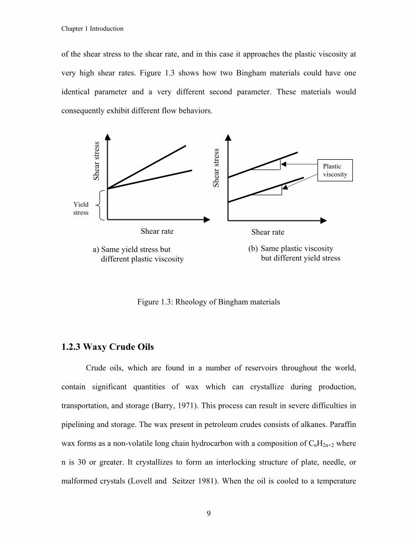


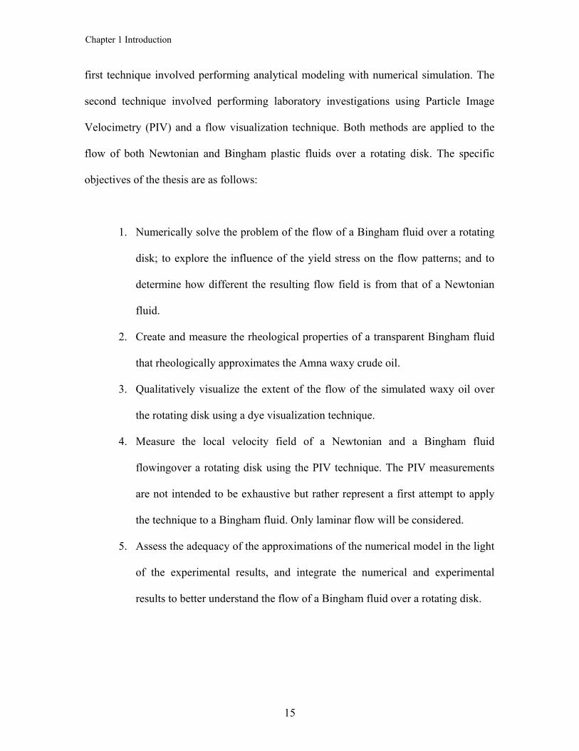


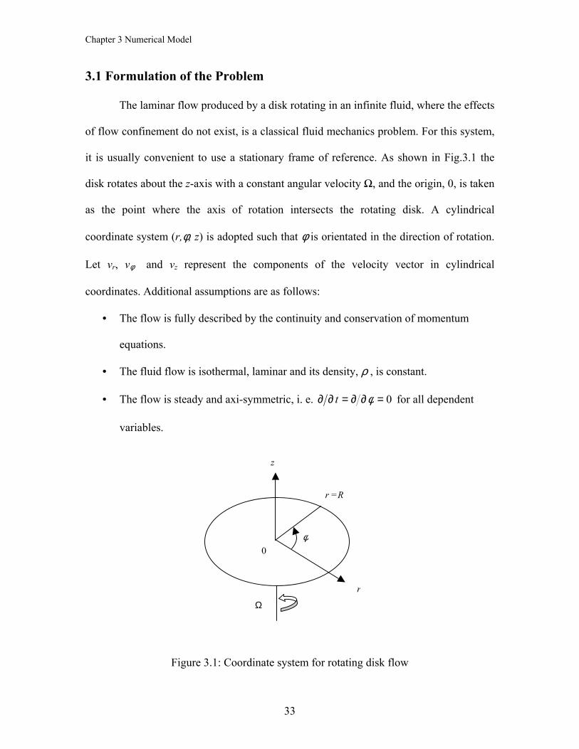


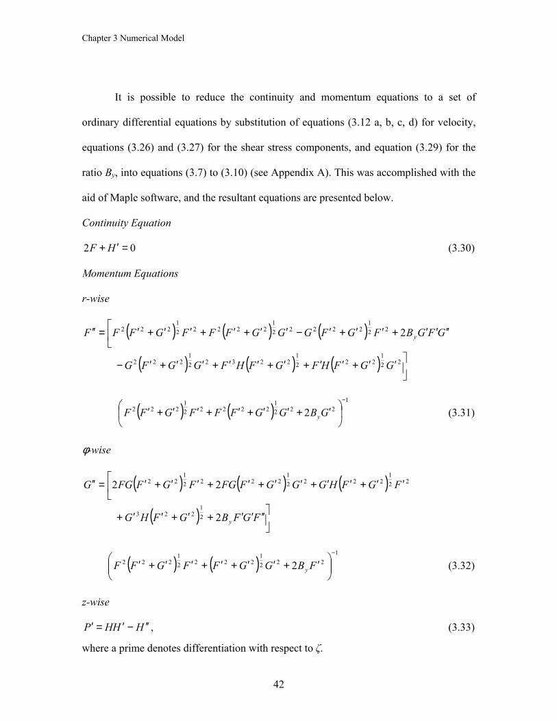


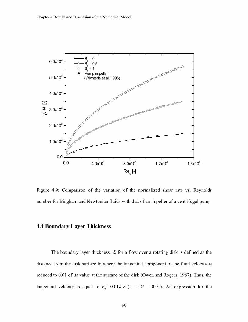
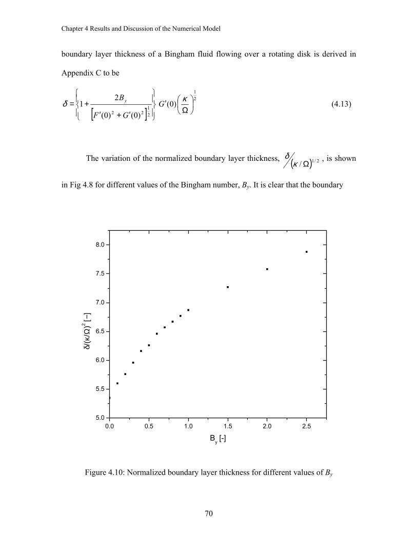


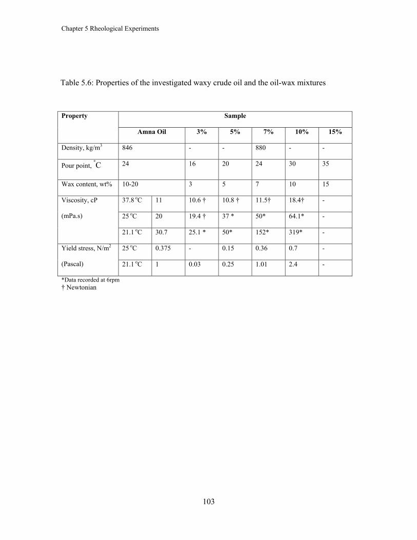


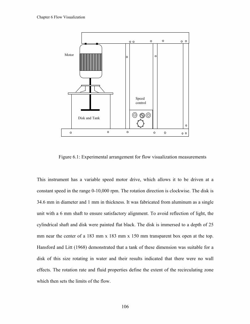


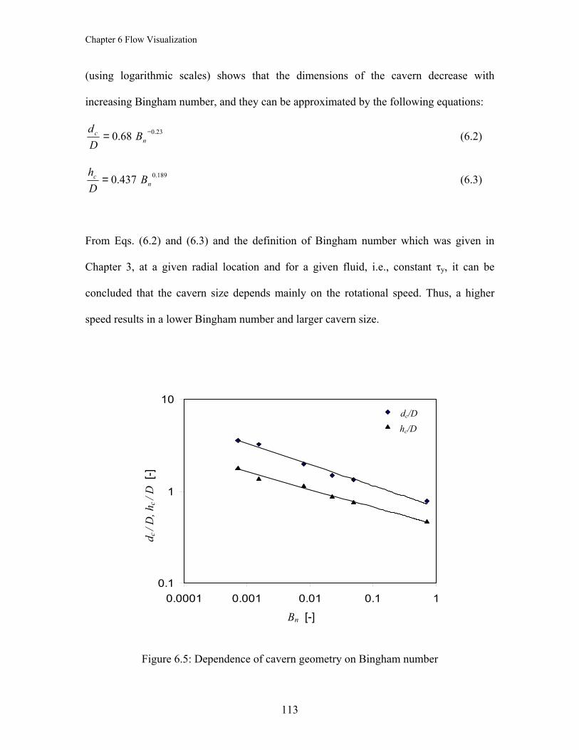


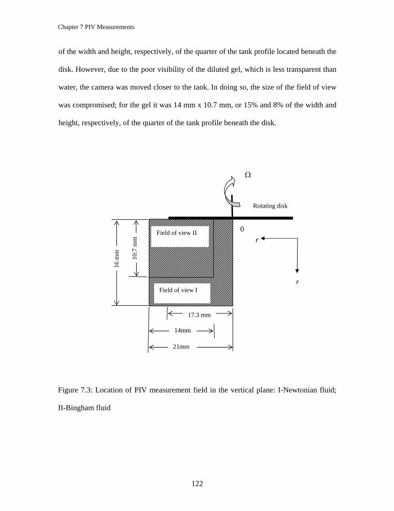


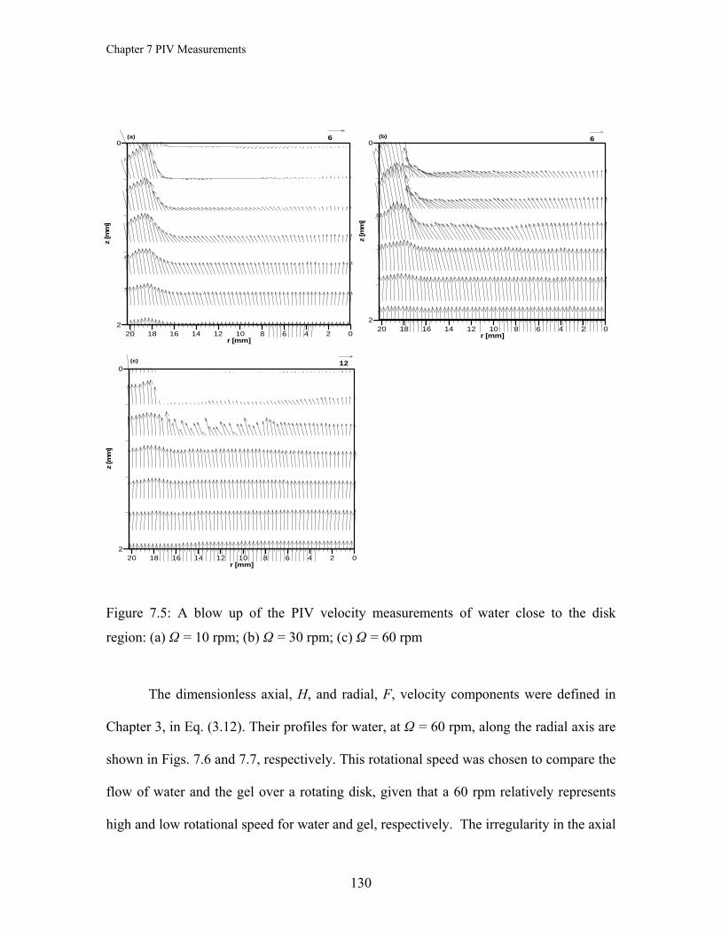
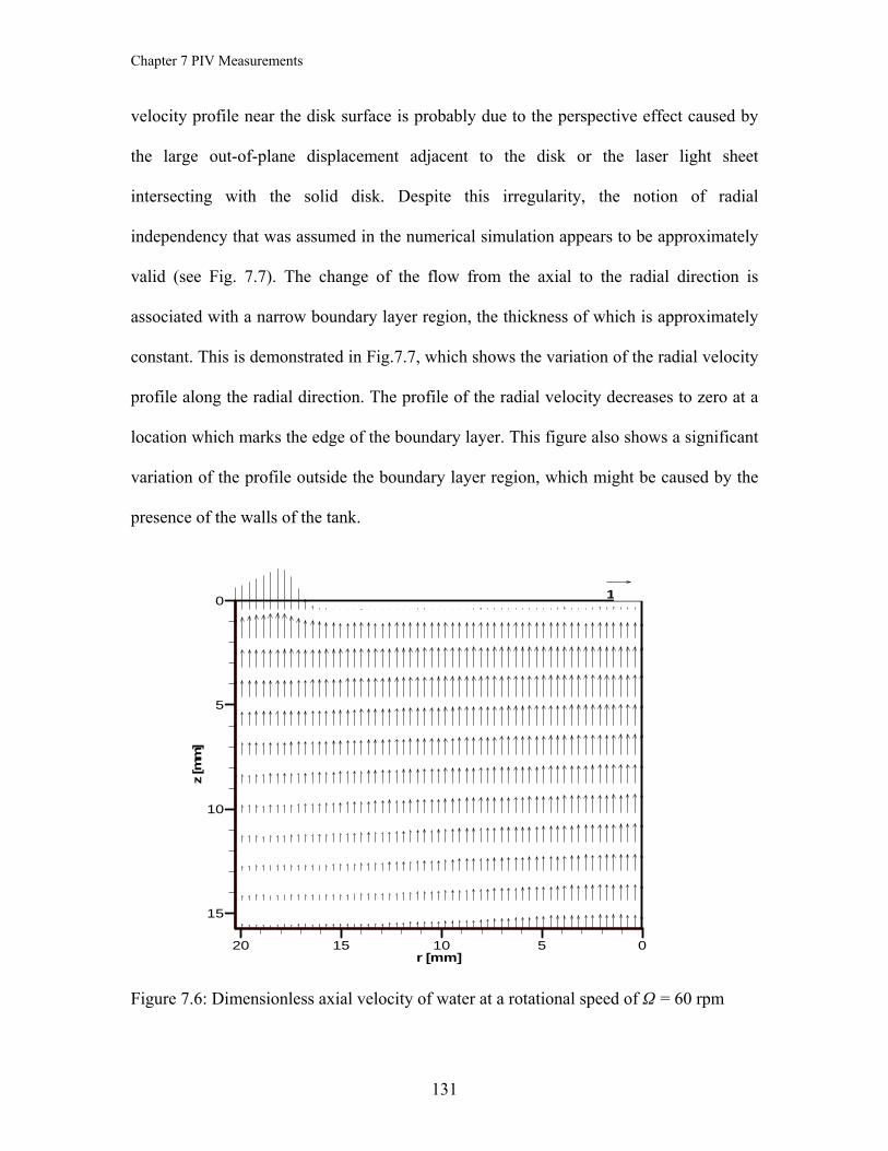


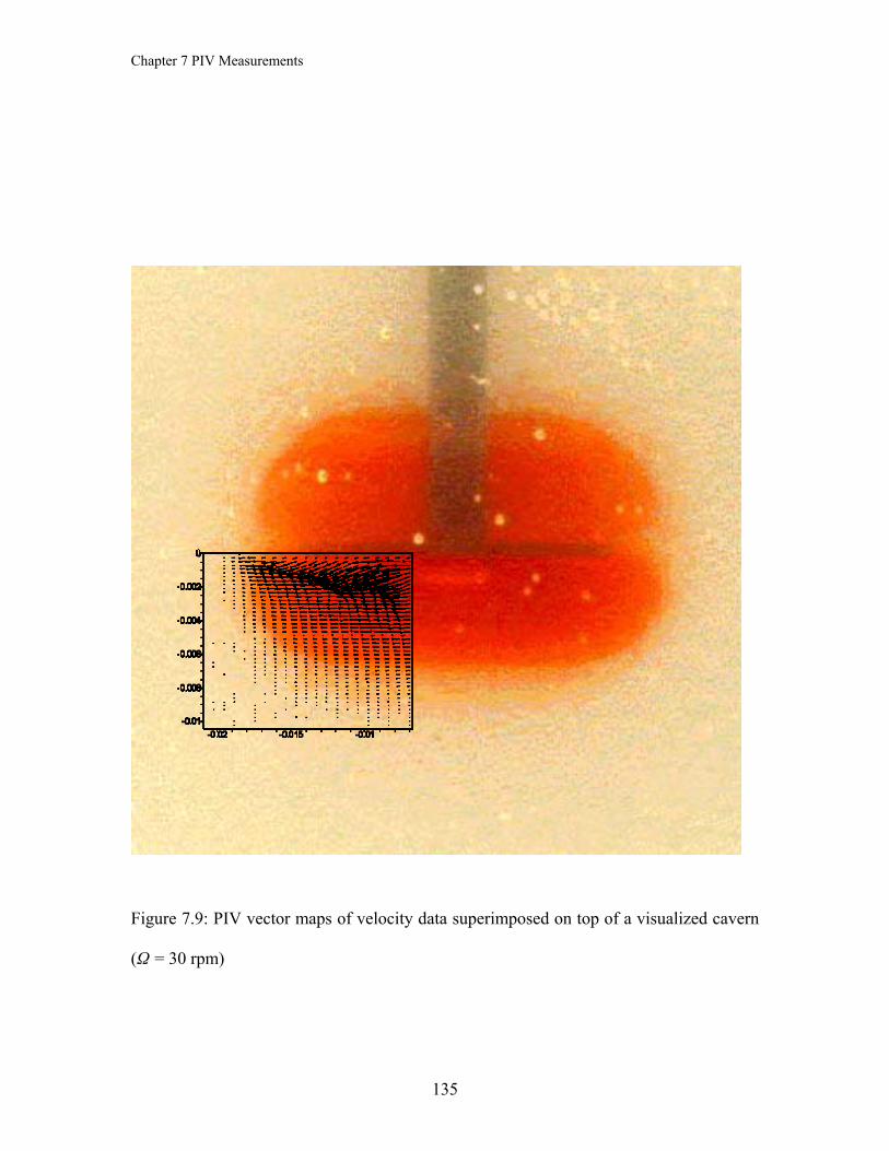

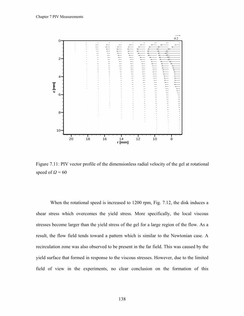


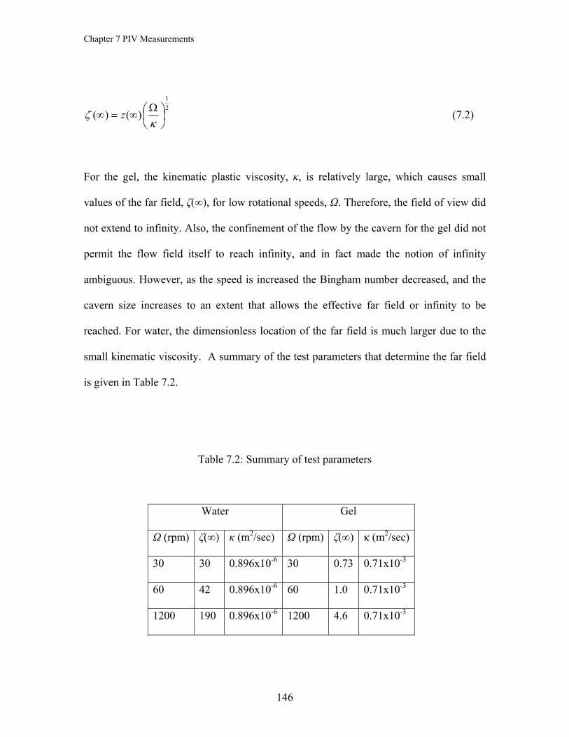


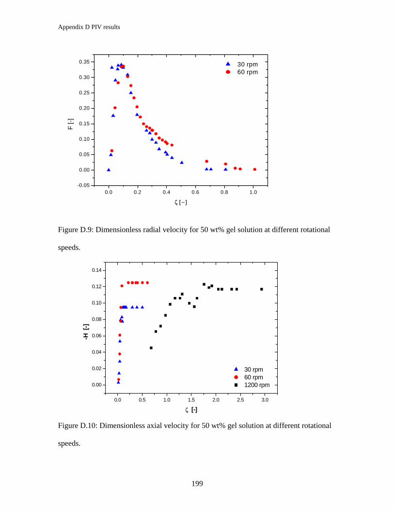


![OPTICAL CHARACTERIZATION OF RARE EARTH …ecommons.usask.ca/bitstream/handle/10388/etd-07292009-064945/Go... · ... Dr. S. O. Kasap, ... Photon Amplification [13] ... Er3+ ion energy](https://static.documents.pub/doc/80x56/5abdc1f17f8b9aa3088c06d3/optical-characterization-of-rare-earth-dr-s-o-kasap-photon-amplification.jpg)


