MASTER'S THESIS Flow Simulations of an Axisymmetric Two- Dimensional 3rd Generation DLE Burner Simon Bruneflod Master of Science in Engineering Technology Space Engineering Luleå University of Technology Department of Engineering Science and Mathematics
Transcript
MASTER'S THESIS
Flow Simulations of an Axisymmetric Two-Dimensional 3rd Generation DLE Burner
Simon Bruneflod
Master of Science in Engineering TechnologySpace Engineering
Luleå University of TechnologyDepartment of Engineering Science and Mathematics
Flow simulations of an axisymmetric two-dimensional 3rd generation DLE burner Master’s thesis in Space Science Engineering
Simon Bruneflod Department of Applied Physics and Mechanical Engineering Division of Fluid Mechanics Luleå University of Technology
Flow simulations of an axisymmetric two-dimensional 3rd generation DLE burner
Simon Bruneflod
Department of Applied Physics and Mechanical Engineering Division of Fluid Mechanics
Luleå University of Technology
I
Acknowledgements My thanks go to people who made this thesis possible. Firstly to Dr. Daniel Lörstad who has been my supervisor at Siemens Industrial Turbomachinery AB. He has guided me towards the right direction and given me a lot of helpful input when I have struggled. Secondly I would like to thank Henrik Hull, also at SIT AB, who gave me the opportunity to come to Siemens which has given me a great insight on how academic work is performed in the industry. I would also like to thank my examiner Staffan Lundström at Luleå University of Technology and last but not least I would like thank friends and family for their support during this time. Finspång May 2010 Simon Bruneflod
II
Abstract In this thesis a parameter study of a gas turbine burner used in the Siemens Gas Turbine SGT-800 and SGT-700 has been performed using computational fluid dynamics. The parameter study was aimed at determining the stability range of the flow field inside the burner and combustion chamber. To perform the study a simplified two dimensional model of the actual burner was developed. The software used for the simulations was Ansys CFX (versions 11.0 and 12.0) and the parameter that has been studied is the swirl number which can be described as a relation between the angular and axial momentum. To change the swirl number scale factors were introduced at the inlet allowing for the velocity profiles to vary. The results showed that the stability range where the flame inside the combustion chamber took the shape of a cone in between the limits of flameback or a rotating jet flame was narrower than assumed from the start. Also the influence of including combustion in the model showed similar results but an even narrower stability range. Besides the parameter study a model has been developed to account for the three dimensional swirling caused by the swirl cone, where forces were applied to force the flow to behave in a certain way. Even though the flow can be mimicked with this approach the fuel distribution in the burner is suffering from some absent three dimensional effect which causes the fuel distribution to be more uniform as compared to simulations made with the axisymmetric model. To validate the simulations the water rig located at Siemens was used where the goal was to examine the radial fuel distribution in five burners. This was done by recording movies of a laser sheet that illuminated water mixed with fluorescence representing fuel. These movies could then be evaluated using MATLAB and comparison to simulations again highlighted the inaccuracy of the fuel distribution in the two-dimensional axisymmetric model. One of the major conclusions of the thesis was that the developed two dimensional axisymmetric model is a valid instrument when performing parameter studies and it is recommended for future studies. When trying to account for the mixing effect of the swirl cone some three dimensional effect is lost and in order to be able to use the complete model of the whole burner this issue has to be resolved.
2.1.1 Conservation of mass...................................................................................... 3 2.1.2 Conservation of momentum............................................................................ 5 2.1.3 The Navier-Stokes equation............................................................................ 8 2.1.4 Conservation of energy................................................................................. 10
2.2 Turbulence ................................................................................... 14 2.2.1 The closure problem ..................................................................................... 16
2.4 The swirl number.......................................................................... 23 2.5 Combustion theory ....................................................................... 24
3 Method..................................................................................... 28 3.1 Grid generation in ICEM.............................................................. 28
3.1.1 Meshing with hexahedrals ............................................................................ 28 3.1.2 Parameter study, cold flow ........................................................................... 30 3.1.3 Parameter study, hot flow ............................................................................. 32 3.1.4 Hood interaction............................................................................................ 33 3.1.5 Holes versus slots.......................................................................................... 33 3.1.6 A mesh of good quality................................................................................. 34
3.2 Pre processing in CFX.................................................................. 36 3.2.1 Parameter study............................................................................................. 38 3.2.2 Combustion settings...................................................................................... 38 3.2.3 Matching of 3D simulations.......................................................................... 39 3.2.4 Hood interaction............................................................................................ 39
IV
3.3 Post processing............................................................................. 40 3.3.1 CFX-post....................................................................................................... 40 3.3.2 MATLAB...................................................................................................... 40
3.4 Water rig experiments .................................................................. 41 3.4.1 Experimental setup........................................................................................ 41 3.4.2 Scaling........................................................................................................... 42 3.4.3 Test objectives .............................................................................................. 43 3.4.4 Test procedure............................................................................................... 44 3.4.5 Post processing.............................................................................................. 45
4 Results...................................................................................... 46 4.1 Parameter study cold flow ............................................................ 46 4.2 Multiple solutions using same boundary conditions...................... 57 4.3 Parameter study hot flow.............................................................. 59 4.4 Matching of 3D simulations ......................................................... 60 4.5 Hood interaction results................................................................ 63 4.6 Water rig results ........................................................................... 67 4.7 Comparison between water rig data and simulations .................... 71
5 Conclusions and discussion ................................................... 72 5.1 Simulations................................................................................... 72 5.2 Water rig ...................................................................................... 73
6 Future Work ........................................................................... 74
1.1 Siemens Industrial Turbomachinery SIT located in Finspång in Sweden develops, manufactures, sells and are responsible for service for their gas and steam turbines all over the world. Their products are used for electricity, steam and heat generation as well as they are used for running pumps and compressors in the oil and gas business. Turbines manufactured by Siemens globally has a power range of 5-340MW whereas SIT in Finspång is responsible for the range 15-50MW
1.2 Background
1.2.1 Gas Turbines A gas turbine consists of three main parts, a compressor, a combustor and a turbine. Compressed air from the compressor enters the combustor burners where it is mixed with fuel before being combusted in the combustion chamber. The hot gas is then expanded through the turbine which is driving the compressor and the rest of the power is harvested in an electric generator or mechanical drive.
1.2.2 Gas turbine burners The burner is where the compressed air mixes with the fuel which is then combusted in the combustion chamber. The most commonly used source for fuel is natural gas but also diesel and other fuels can be used. The mixing and combustion is a crucial part to the gas turbine performance where features such as flameback and high levels of combustion dynamics are undesired. Also there is always a goal to reduce nitrogen oxides to minimize the contribution to the acid rain effect as well as carbon monoxide and unburnt hydrocarbons. The focus of this thesis is in the gas turbine burner which is mounted in two of SIT’s largest gas turbines namely the SGT-700 and the SGT-800 and it is called “3rd generation Dry Low Emission burner” or in short “3rd gen. DLE” as it will be referred throughout the text.
1.2.3 Computational Fluid Dynamics (CFD) CFD is the method of using computers to solve and analyze problems that involve fluid flows. The method of solving partial differential equations using numerical models have until recent years not been of practical use but due to the rapid development of computer power, CFD has been widely adopted throughout both the academic and the industry world. Still there are many simplifications to the many equations to be solved but ongoing research and further development of computers both contributes to increasing accuracy and speed for given problems. Generally the way in which computers deal with continuous flows is to discretize the domain of interest into small subdomains using a technique called Finite Volume Method (FVM) where the equations can be solved for each volume individually.
2
1.2.4 Thesis background In the 3rd gen DLE burner the flow is swirling in order to achieve a vortex breakdown at the burner outlet where the flame may stabilize. There is a mixing tube to obtain good mixing quality between the fuel and the compressed air that enters the burner. The swirling flow results in, when the flow enters the combustion chamber, a cone shaped flame. This cone shape only occurs within an undefined range where if the swirl is too high the flame would creep upstream towards the burner and if the swirl is to low the flame would take the shape of a rotating jet. Therefore a parameter study was necessary in which the goal was to determine the range in which the flame takes the shape of the desired cone. In order to allow for an efficient parameter study there was a need for a simplified model, that also may be used in future investigations of more advanced combustion models.
1.3 Thesis Goals The goals of the thesis was to apply an axisymetric simplification that required low amount of computer resources but also gave accurate results. This simplified model should be a representation of the 3rd gen DLE burner applied in the Finspång Atmospheric Combustion Rig. The parameter study was aimed at determining the influence of both the magnitude of the swirl number but also the shape and relation between the tangential and axial velocity profiles inside the burner. The difference between cold and hot flow i.e. when combustion was added was also to be evaluated. Apart from the parameter study there was also a desire to produce a model which would represent all parts of the burner including the swirl cone, which in reality is the source of the swirling flow. This effect would need modeling when using the simplified axisymmetric model. There is always a desire to compare simulation results with experimental data and therefore another goal of the thesis was to obtain experimental data from the water rig in the fluid dynamic laboratory in Finspång. Here the goal was to extract radial profiles of the fuel distribution inside the 3rd gen DLE burner.
3
2 Theory In this chapter the governing equations for a fluid is described. These equations are the conservation of mass, momentum and energy.
2.1 Conservation laws
2.1.1 Conservation of mass The conservation of mass is one of the most fundamental principles in nature. It states that, for a closed system the mass of the system remain constant throughout a process. More related to fluid dynamics it states that the net rate at which mass flows into a control volume is equal to the net rate at which mass flows out of the control volume. This put into an equation valid for any control volume regardless of size
∑∫ ∑ −=∂∂
outCV in
mmdVt
&&ρ
( 2.1 )
Consider an infinitesimal box-shaped control volume with the dimensions dx, dy and dz in a Cartesian coordinate system. At the centre of the volume the density ρ and the three velocity components u, v and w is defined. The mass flux in the x-direction and at the centre of the volume is then uρ and the corresponding mass flux in y- and z-direction is
vρ and wρ To find the mass flux through each face of the volume a Taylor expansion is used
( )...
2!2
1
2
)()(
2
2
2
faceright ofcenter +
∂+∂
∂+= dx
dx
udx
x
uuu
ρρρρ ( 2.2 )
Terms of second order and higher are negligible when the control volume shrinks sufficiently. Applying this to all six faces we end up with
2
)()(:face bottom ofCenter
2
)()(:face topofCenter
2
)()(:facerear ofCenter
2
)()(:facefront ofCenter
2
)()(:faceleft ofCenter
2
)()(:faceright ofCenter
face bottom ofcenter
face topofcenter
facerear ofcenter
facefront ofcenter
faceleft ofcenter
faceright ofcenter
dy
y
vvv
dy
y
vvv
dz
z
www
dz
z
www
dx
x
uuu
dx
x
uuu
∂∂−≅
∂∂+≅
∂∂−≅
∂∂+≅∂
∂−≅∂
∂+≅
ρρρ
ρρρ
ρρρ
ρρρ
ρρρ
ρρρ
( 2.3 )
4
The mass flow rate through one of the faces is equal to the density times the normal velocity at the centre of the face and times the area of the face
AVm nρ=& ( 2.4 )
The net mass flow rate through each face of the control volume is made visible in Figure 2.1. The velocity components are assumed positive in their respective direction but even if the opposite was the case the derivation would yield the same result.
For a sufficiently small control volume yields
dxdydzt
dVtCV ∂
∂≅∂∂∫
ρρ ( 2.5 )
We can now apply the approximations of Figure 2.1 to equation 2.1 The mass flow rate entering the control volume is
dxdydz
z
wwdxdz
dy
y
vvdydz
dx
x
uum
in 444 3444 2144 344 2144 344 21
&
facerear face bottomfaceleft
2
)(
2
)(
2
)(
∂∂−+
∂∂−+
∂∂−≅∑
ρρρρρρ ( 2.6 )
The mass flow rate going out from the control volume is similarly
Figure 2.1: Mass flux through the faces of a control volume.
5
dxdydz
z
wwdxdz
dy
y
vvdydz
dx
x
uum
out 444 3444 2144 344 2144 344 21
&
facefront face topfaceright
2
)(
2
)(
2
)(
∂∂++
∂∂++
∂∂+≅∑
ρρρρρρ ( 2.7 )
Substituting equation 2.5, 2.6 and 2.7 into equation 2.1 and simplifying where most terms disappear we end up with
dxdydzz
wdxdydz
y
vdxdydz
x
udxdydz
t ∂∂−
∂∂−
∂∂−=
∂∂ )()()( ρρρρ
( 2.8 )
Dividing by the volume dxdydz we end up with the following differential equation for conservation of mass, also known as the continuity equation in Cartesian coordinates
0)()()( =
∂∂+
∂∂+
∂∂+
∂∂
z
w
y
v
x
u
t
ρρρρ ( 2.9 )
This equation written in a more compact form
( ) 0=∇+∂∂
Vt
ρρ ( 2.10 )
And for incompressible flow [1]
0=⋅∇ V ( 2.11 )
2.1.2 Conservation of momentum To derive the equation for conservation of momentum, we apply Newton’s second law to a material element. To do this we need to know how the material acceleration is described. In a lagrangian description of a fluid particle the location in space is written as a material position vector
)(
)(
)(
particle
particle
particle
tz
ty
tx
If we apply Newton’s second law to this fluid particle we have
particleparticleparticle amF = ( 2.12 )
6
Where particleF is the net force acting on the fluid particle, particlem is its mass, and particlea is
its acceleration. The acceleration is defined as the derivative of the particle’s velocity
dt
Vda particle=particle ( 2.13 )
At any instant time the velocity of the particle is the same as the local velocity field at the particle’s position. Applying the chain rule yields
dt
dz
z
V
dt
dy
y
V
dt
dx
x
V
dt
dt
t
V
dt
tzyxVd
dt
Vda particle
particle
particle
particle
particle
particle
particle
particle,particle,particle,particle
)(
∂∂+
∂∂+
∂∂+
∂∂=
== ( 2.14 )
Considering that dtdxparticle is the x-component of the velocity vector u and similarly
vdtdyparticle = and wdtdzparticle = . Furthermore the material position vector
),,( particleparticleparticle zyx in the lagrangian frame corresponds to ),,( zyx in the eulerian
frame. Now rewriting equation 2.13
z
Vw
y
Vv
x
Vu
t
V
dt
Vdtzyxa
∂∂+
∂∂+
∂∂+
∂∂==),,,(particle ( 2.15 )
Finally the acceleration field at any given time t must be equal to the acceleration of the particle at that time and space so
),,,(particle tzyxaa = ( 2.16 )
Writing this in vector form we end up with
( )VVt
V
dt
Vdtzyxa ∇⋅+
∂∂==),,,( ( 2.17 )
which is the acceleration of a fluid particle expressed as a field variable. The material derivative d/dt, or the total derivative operator in equation 2.17 is often written as
)( ∇⋅+∂∂== Vtdt
d
Dt
D ( 2.18 )
7
So the material acceleration in a more compact form is written as
Dt
VDtzyxa =),,,( ( 2.19 )
Applying Newton’s second law a material element of fluid
Dt
VDdxdydz
Dt
VDmamF ρ===∑ ( 2.20 )
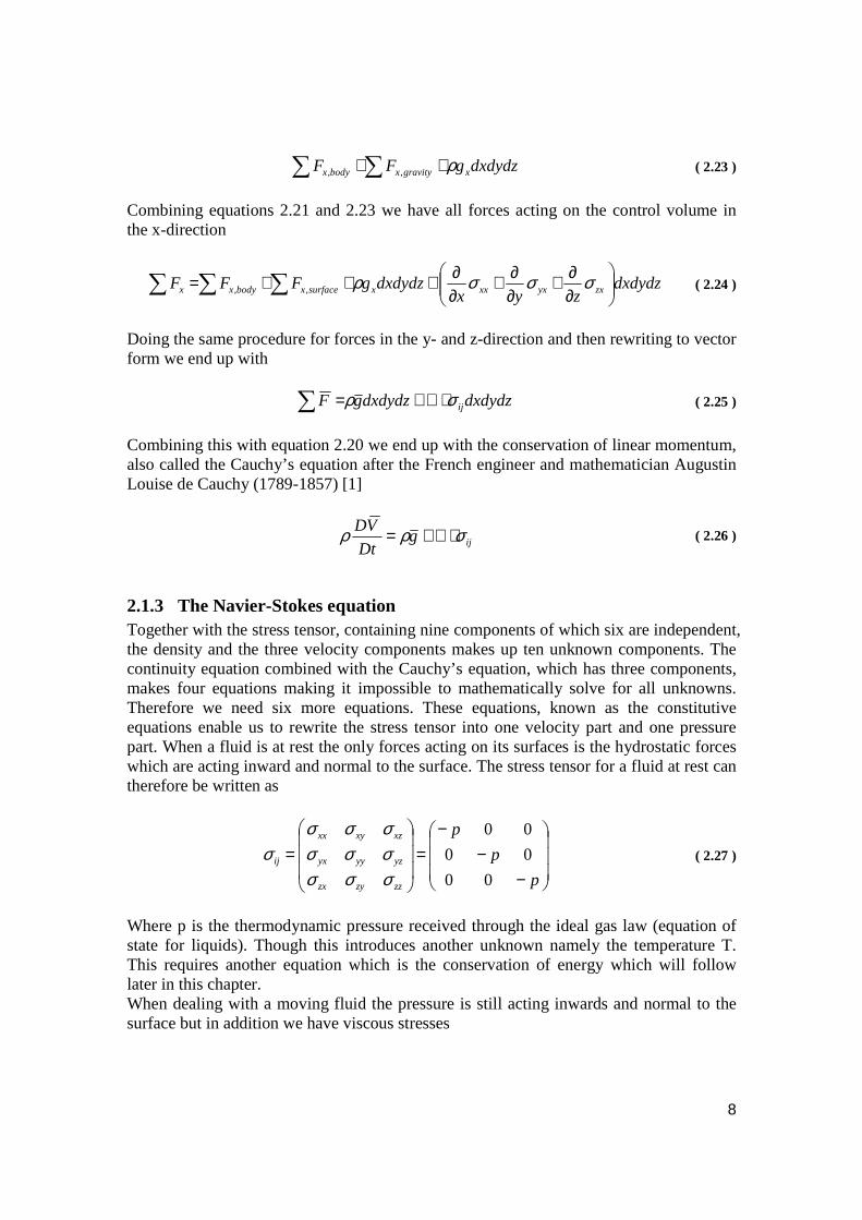
At an instant time the net force acting on a fluid element is the same as the force acting on a control volume. In Figure 2.2 the surface forces acting on a control volume in the x-direction is visualized. The same truncated Taylor series expansion is used as when the conservation of mass was derived earlier which means that the terms of second order and higher are disregarded.
Summing the net surface forces acting on the control volume in the x-direction
∑
∂∂+
∂∂+
∂∂≅ dxdydz
zyxF zxyxxxsurfacex σσσ, ( 2.21 )
The gravity vector is acting on the control volume as a body force and is written
kgjgigg zyx ++= ( 2.22 )
So the body force acting on the control volume in the x-direction is
Figure 2.2: The forces in x-direction acting on each surface o the control volume.
8
dxdydzgFF xgravityxbodyx ρ∑∑ ≅≅ ,, ( 2.23 )
Combining equations 2.21 and 2.23 we have all forces acting on the control volume in the x-direction
dxdydzzyx
dxdydzgFFF zxyxxxxsurfacexbodyxx
∂∂+
∂∂+
∂∂+≅+= ∑∑∑ σσσρ,, ( 2.24 )
Doing the same procedure for forces in the y- and z-direction and then rewriting to vector form we end up with
dxdydzdxdydzgF ijσρ ⋅∇+=∑ ( 2.25 )
Combining this with equation 2.20 we end up with the conservation of linear momentum, also called the Cauchy’s equation after the French engineer and mathematician Augustin Louise de Cauchy (1789-1857) [1]
ijgDt
VD σρρ ⋅∇+= ( 2.26 )
2.1.3 The Navier-Stokes equation Together with the stress tensor, containing nine components of which six are independent, the density and the three velocity components makes up ten unknown components. The continuity equation combined with the Cauchy’s equation, which has three components, makes four equations making it impossible to mathematically solve for all unknowns. Therefore we need six more equations. These equations, known as the constitutive equations enable us to rewrite the stress tensor into one velocity part and one pressure part. When a fluid is at rest the only forces acting on its surfaces is the hydrostatic forces which are acting inward and normal to the surface. The stress tensor for a fluid at rest can therefore be written as
−−
−=
=p
p
p
zzzyzx
yzyyyx
xzxyxx
ij
00
00
00
σσσσσσσσσ
σ ( 2.27 )
Where p is the thermodynamic pressure received through the ideal gas law (equation of state for liquids). Though this introduces another unknown namely the temperature T. This requires another equation which is the conservation of energy which will follow later in this chapter. When dealing with a moving fluid the pressure is still acting inwards and normal to the surface but in addition we have viscous stresses
9
+
−−
−=
=
zzzyzx
yzyyyx
xzxyxx
zzzyzx
yzyyyx
xzxyxx
ij
p
p
p
τττττττττ
σσσσσσσσσ
σ00
00
00
( 2.28 )
Where ijτ is the viscous stress tensor. This is not helping the situation replacing
unknowns with new unknowns but the viscous stresses can be derived through knowledge of the velocity field and viscosity of the fluid. Throughout these derivations the fluid is considered being a Newtonian fluid i.e. the shear stress is linearly proportional to the shear strain rate. This put into an equation gives
ijij µετ 2= ( 2.29 )
Where ijε is the strain rate tensor so
∂∂
∂∂+
∂∂
∂∂+
∂∂
∂∂+
∂∂
∂∂
∂∂+
∂∂
∂∂+
∂∂
∂∂+
∂∂
∂∂
+
−−
−=
z
w
z
v
y
w
z
u
x
w
y
w
z
v
y
v
y
u
x
v
x
w
z
u
x
v
y
u
x
u
p
p
p
ij
µµµ
µµµ
µµµ
σ
2
2
2
00
00
00
( 2.30 )
Using the assumption that the fluid considered is incompressible and that the variations of the temperature are small enough to be disregarded we will end up with Navier-Stokes equation for incompressible isothermal flow. Using the expression for the stress tensor in equation 2.30 considering the x-component only we have
∂∂+
∂∂
∂∂+
∂∂+
∂∂
∂∂+
∂∂+
∂∂−
=⋅∇+=
z
u
x
w
zy
u
x
v
yx
u
x
pg
gDt
Du
x
ij
µµµρ
σρρ
2
2
2 ( 2.31 )
Noting that
∂∂
∂∂=
∂∂
∂∂
z
w
xx
w
zµµ ( 2.32 )
Some rearranging can be done to equation 2.31
10
∂∂+
∂∂+
∂∂+
∂∂+
∂∂+
∂∂
∂∂++
∂∂−=
2
2
2
2
2
2
z
u
y
u
x
u
z
w
y
v
x
u
xg
x
p
Dt
Dux µρρ ( 2.33 )
According to the continuity equation the first part inside the parenthesis is equal to zero and the second part is the Laplacian of the velocity component u. Rewriting this in vector format gives
ugx
p
Dt
Dux
2∇++∂∂−= µρρ ( 2.34 )
Using the same procedure for the y- and z-component and finally rewriting we end up with the Navier-Stokes equation for incompressible isothermal flow
VgpDt
VD 2∇++−∇= µρρ ( 2.35 )
This equation is named after Louis Marie Henri Navier (1785-1836) and Sir George Gabriel Stokes (1819-1903) who both developed the viscous terms independent of each other. It is an unsteady, nonlinear partial differential equation of the second order which is very hard to solve for even the simplest flows. [1]
2.1.4 Conservation of energy When dealing with incompressible flows the continuity and the momentum equations are sufficient to solve for the unknowns p and V . Though when the flow is compressible, as is the case in a gas turbine, two more unknowns arise namely the internal energy eand the temperatureT . Therefore the first law of thermodynamics stating that Energy can be neither created nor destroyed: It can only change in form This means that the rate of change of energy inside the fluid element is equal to the net flow of heat into the element plus the rate of work done on the element (using the lagrangian description).
WQdE ∂+∂= ( 2.36 )
Starting with the final term, i.e. the work term, we know that the rate of work done on a fluid is a force times the velocity component in the direction of the force so the body force work on our element is
dxdydzVfρ ( 2.37 )
The work done on the surfaces by shear and normal stresses are identified by again looking at Figure 2.2. The addition from the shear stresses in the x-direction is
11
( ) ( ) dxdzdy
uy
udxdzdy
uy
u yxyxyxyx
⋅
∂∂−−
⋅
∂∂+
22σσσσ ( 2.38 )
And
( ) ( ) dxdydz
uz
udxdydz
uz
u zxzxzxzx
⋅∂∂−−
⋅∂∂+
22σσσσ ( 2.39 )
The addition from the normal stresses is
( ) ( ) dydzdx
ux
udydzdx
ux
u xxxxxxxx
⋅∂∂−−
⋅∂∂+
22σσσσ ( 2.40 )
Also needed to be included is the work done due to pressure forces and that is
( ) ( ) dydzdx
pux
pudydzdx
pux
pu
⋅∂∂−−
⋅∂∂+
22 ( 2.41 )
Summing equations 2.38-2.41, simplifying and dividing by the volume dxdydz
( ) ( ) ( ) ( )pux
uz
uy
ux zxyxxx ∂
∂−∂∂+
∂∂+
∂∂ σσσ
If solving in the same way for the y- and z-direction summing all terms, including equation 2.37, we end up with
( ) ( ) ( )
( ) ( ) ( )
( ) ( ) ( )
( ) ( ) ( )
Vf
pwz
pvy
pux
wz
wy
wx
vz
vy
vx
uz
uy
ux
zzyzzx
zyyyyx
zxyxxx
ρ
σσσ
σσσ
σσσ
+
∂∂+
∂∂+
∂∂+
+
∂∂+
∂∂+
∂∂+
+
∂∂+
∂∂+
∂∂+
+
∂∂+
∂∂+
∂∂
...
......
......
...
( 2.42 )
The first term on the right hand side of equation 2.36 represents the net flow of heat into the element and it can be divided into two parts. The volumetric heating, i.e. radiation and combustion, and the heat transfer across the surfaces due to temperature gradients, i.e.
12
conduction. Starting with the volumetric heating, if the heat flux vector is defined asq& we have
dxdydzq&ρ ( 2.43 )
The heat flux through the surfaces of the control volume is presented in Figure 2.3 and is analogous with the derivation of the mass flux in the conservation of mass section. The net heat transferred by thermal conduction through the faces with a normal in the x-direction is
dxdydz
z
qqdxdy
dz
z
qq z
zz
z
∂∂+−
∂∂−
22
&&
&& ( 2.44 )
Taking the other directions into account as well as the volumetric heating, simplifying the equations and dividing by the fluid volume we end up with
∂∂+
∂∂
+∂∂−
z
q
y
q
x
qq zyx &&&&ρ ( 2.45 )
The heat flux is related to the temperature through Fourier’s law of heat conduction
Figure 2.3: The heat flux through the surfaces of the control volume.
13
Tkq ∇−=& ( 2.46 )
Where k is the thermal conductivity and T is the temperature. Now by applying this relation on equation 2.45 we have
∂∂
∂∂+
∂∂
∂∂+
∂∂
∂∂+
z
Tk
zy
Tk
yx
Tk
xq&ρ ( 2.47 )
Writing the total rate of change of energy with the material derivative we now have a complete description, in vector form, saying [2]
( ) ( ) ( ) VfpVpVTkqDt
DEij +∇+⋅∇−⋅∇⋅∇+= σρρ & ( 2.48 )
14
2.2 Turbulence Dealing with turbulent flows, which is almost always the case, makes the CFD calculations more difficult than in a laminar case. The reason for this is that the features of turbulence introduces three-dimensional, rapid, unsteady and nonlinear so called eddies. The time- and length scales of these eddies can differ in several orders of magnitude and they can be found in all directions of the flow which is the reason for the difficulty introduced to simulations. There are a few ways on how to calculate turbulence in CFD and a brief description will be made to some of them. The direct numerical simulation (DNS) tries to solve the motions for all scales of the turbulence. Therefore a DNS simulation relies heavily on an extremely fine grid that requires extremely powerful computers. This makes the DNS hardly useful when simulating even the simplest flow and if the Reynolds number is high the turbulence in the flow increases which makes it even harder. The large eddy simulation (LES) resolves the motion for the larger eddies in the flow leaving the smaller scale eddies to be modelled. This is done with the assumption that the smaller eddies are isotropic i.e. they are assumed to behave in a statistically predictable way regardless of the turbulent flow field. The LES demands much less computer resources compared to DNS but still the requirement is significant. The most practical way so far has been to model all the turbulent eddies with a specific turbulence model. In this case none of the eddies are resolved, not even the largest ones but instead the features of turbulence i.e. enhanced mixing and diffusion is modelled. Using such a turbulence model means the Navier-Stokes equation is replaced by a Reynolds-averaged Navier-Stokes equation (RANS). In CFD always compromises need to be done regarding accuracy and resolution of the solution and the computational- and time resources at hand. In this thesis the turbulence have been dealt with using the RANS equation so a description on how this is derived is therefore presented. If expanding the incompressible Navier-Stokes equation for the x-direction we have (note that the body force is assumed to be zero)
( ) ( ) ( )
∂∂+
∂∂+
∂∂+
∂∂−=
∂∂+
∂∂+
∂∂+
∂∂
2
2
2
2
2
22
z
u
y
u
x
u
x
puw
zuv
yu
xt
u µρ ( 2.49 )
A technique to separate the time or ensemble averaged mean- and the fluctuating part of a quantity is called Reynolds decomposition and is written
'φφφ += ( 2.50 )
15
Time averaging models a turbulent steady flow for a certain time interval while the ensemble averaging technique models a turbulent flow at several different occasions and taking the average of the process. These techniques are defined as
average Ensemble
1
average Time
0
1
1∑∫ =
∆=
∆ Nt
Ndt
tφφφφ ( 2.51 )
Looking at the second term on the left hand side and applying the decomposition theory we have
( ) ( )2222 ''2')( uuuux
uux
ux
++∂∂=+
∂∂=
∂∂
( 2.52 )
The way to derive the RANS equations is to time or ensemble average the unsteady Navier-Stokes and looking at the average of the equation above we get
( )22 ''2 uuuux
++∂∂
( 2.53 )
The first part inside the derivative is independent of averaging so its averaged value is equal to the independent quantity. Since the average of 'u is equal to zero so is the second term of the derivative. Finally the last term is an always positive oscillating value with
the average 2'u so the result is
( ) ( )2222 '''2 uux
uuuux
+∂∂=++
∂∂
( 2.54 )
Noting also that the first term on the left hand side in equation 2.49 is equal to zero when time averaging, using a sufficiently long ∆t in equation 2.51, since u has a zero time derivative and the time average of 'u is also zero. However, when using ensemble
averaging the transient term remain tutu ∂∂=∂∂ . The third term on the left hand side, when averaged, is
( )( )[ ] ( ) ( )'''''''')( vuvuy
vuuvvuvuy
vvuuy
uvy
+∂∂=+++
∂∂=++
∂∂=
∂∂
( 2.55 )
With the same procedure the last term of the left hand side becomes
( )'')( wuwuz
uwz
+∂∂=
∂∂
( 2.56 )
16
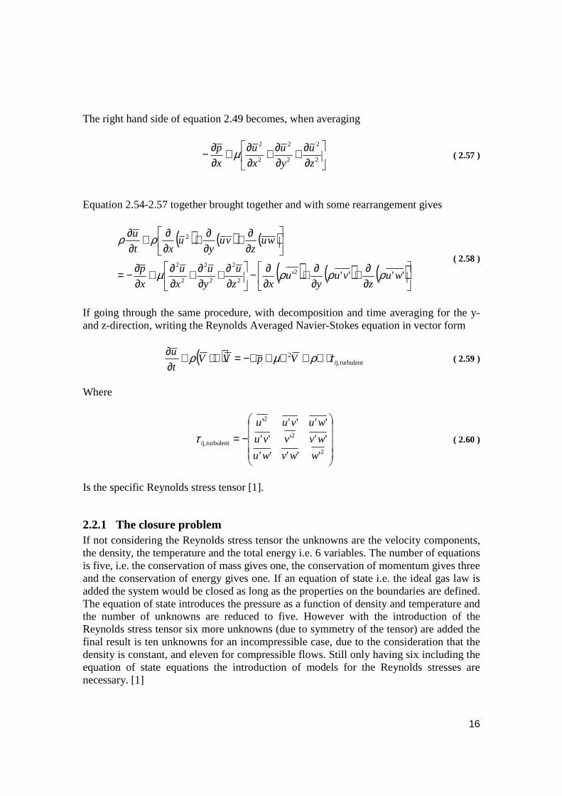
The right hand side of equation 2.49 becomes, when averaging
∂∂+
∂∂+
∂∂+
∂∂−
2
2
2
2
2
2
z
u
y
u
x
u
x
p µ ( 2.57 )
Equation 2.54-2.57 together brought together and with some rearrangement gives
( ) ( ) ( )
( ) ( ) ( )
∂∂+
∂∂+
∂∂−
∂∂+
∂∂+
∂∂+
∂∂−=
∂∂+
∂∂+
∂∂+
∂∂
'''''22
2
2
2
2
2
2
wuz
vuy
uxz
u
y
u
x
u
x
p
wuz
vuy
uxt
u
ρρρµ
ρρ ( 2.58 )
If going through the same procedure, with decomposition and time averaging for the y- and z-direction, writing the Reynolds Averaged Navier-Stokes equation in vector form
( ) turbulentj,2
iVpVVt
u τρµρ ⋅∇+∇+−∇=∇⋅+∂∂
( 2.59 )
Where
−=2
2
2
turbulentj,
'''''
'''''
'''''
wwvwu
wvvvu
wuvuu
iτ ( 2.60 )
Is the specific Reynolds stress tensor [1].
2.2.1 The closure problem If not considering the Reynolds stress tensor the unknowns are the velocity components, the density, the temperature and the total energy i.e. 6 variables. The number of equations is five, i.e. the conservation of mass gives one, the conservation of momentum gives three and the conservation of energy gives one. If an equation of state i.e. the ideal gas law is added the system would be closed as long as the properties on the boundaries are defined. The equation of state introduces the pressure as a function of density and temperature and the number of unknowns are reduced to five. However with the introduction of the Reynolds stress tensor six more unknowns (due to symmetry of the tensor) are added the final result is ten unknowns for an incompressible case, due to the consideration that the density is constant, and eleven for compressible flows. Still only having six including the equation of state equations the introduction of models for the Reynolds stresses are necessary. [1]
17
2.3 Turbulence models There are three approaches to compute the Reynolds stresses
The third one, itself having three different subcategories, is the most commonly used but in this theses the Reynolds stress model has also been used as comparison [4].
2.3.1 Reynolds stress model Since the eddy viscosity models originates from the description for the Reynolds stress equation this will be described first. To describe the fluctuations in motion we again use the Reynolds decomposition theory on the incompressible momentum equation which yields
ij
ij
j
ij
i
x
p
xx
uu
t
u
∂∂−
∂∂
=
∂∂+
∂∂ τ
ρ ( 2.61 )
And the result is
( ) ( ) ( ) ( ) ( )ij
ijij
j
iijj
ii
x
pp
xx
uuuu
t
uu
∂+∂−
∂+∂
=
∂+∂++
∂+∂ '''
'' ττ
ρ ( 2.62 )
After ensemble averaging equation 2.62 we end up with
j
ij
ij
ij
j
ij
i
x
uu
x
p
xx
uu
t
u
∂∂−
∂∂−
∂∂
=
∂∂+
∂∂ '
'ρτ
ρ ( 2.63 )
Subtracting equation 2.63 from equation 2.49 yields an equation for the fluctuation as
∂∂−
∂∂−
∂∂−
∂∂−
∂∂
=
∂∂+
∂∂
j
ij
j
ij
j
ij
ij
ij
j
ij
i
x
uu
x
uu
x
uu
x
p
xx
uu
t
u ''
'''
'''' ρρτ
ρ ( 2.64 )
Multiplying equation 2.64 with ku' and performing several mathematical operations we end up with the final result, the Reynolds stress equation.
18
[ ] [ ]{ }
∂∂+
∂∂−
∂∂+
∂∂−
++−+−∂∂+
∂∂+
∂∂−=∂+
∂∂
j
ikj
j
kij
j
ijk
j
kji
kijkijjkiijiijkj
k
i
k
i
j
kij
ki
x
us
x
us
x
uuu
x
uuu
ususuuupupux
x
u
x
up
x
uuu
t
uu
''2
''''
''2'''''
''''''
ν
νδδ
ρ
( 2.65 )
The term on the left hand side in equation 2.65 is the rate of change of Reynolds stress following the mean motion whereas the terms on the right hand side are starting from the left, the pressure-strain rate term, the turbulence transport term, the production term and the dissipation term. All terms except the production term has to be modelled when using the Reynolds stress model in the designated software used for analysis. This is due to the introduction of 75 new unknowns that in turn have to be modelled even though most of them are not independent. A full description on how the Reynolds stress equation is used to formulate the Reynolds stress model is beyond the scope of this thesis but it can be said that even though theoretically a Reynolds stress model has the potential to model complex flows they are often not superior to the following two equation models based on the eddy viscosity hypothesis. [4] In addition the Reynolds stress model are often connected with large convergence difficulties.
2.3.2 Linear eddy viscosity models There are three subcategories to the linear eddy viscosity models namely
1. Algebraic models or zero equation models 2. One equation models 3. Two equation models
The one thing that these models have in common is the modelling of the Reynolds stresses by a linear constitutive relationship with the mean flow as
ijijtij kS δρµρτ3
22turbulent, −=− ( 2.66 )
Where tµ is the eddy viscosity, ijS is the mean strain rate and k is the mean turbulent
kinetic energy written as
)'''(2
1 222 wvuk ++= ( 2.67 )
19
This assumption is known as the Boussinesq hypothesis. With this formulation the question of finding the unknown Reynolds stresses is replaced by the task of finding a model for the eddy viscosity. The Boussinesq hypothesis is based on the assumption that turbulence in the averaged sense acts as addition variable viscosity of the flow due to the diffusive behaviour of turbulence. In complex flows with high vorticity this assumption is not valid and these type of models should be used with care. The zero equation models and the one equation models have not been used in this thesis and are therefore not derived but a short note will be presented. In the zero equation models the eddy viscosity is constant for the entire flow which proposes a model with very little physical foundation and is not recommended for other situations where there might be difficulties to get initial values for a flow. One equation turbulence models solve one turbulent transport equation, usually the turbulent kinetic energy while modelling the eddy viscosity.
20
Two equation models The two equation models are the most commonly used models for turbulence for engineering problems. They introduce two new transport equations that represent the turbulent properties of the flow and hence you can account for history effects like convection and diffusion of turbulent energy. The most common transported variables are the turbulent kinetic energy and, depending on what two equation model you are using, either the turbulent dissipation or the turbulent specific dissipation. The second variable can be thought of as the variable that determines the length- or time scale of the turbulence. In the two equation models the eddy viscosity is assumed to be linked with the kinetic energy via
ερµ
2kCt = ( 2.68 )
The k-ε model If modelling with a k-ε model the values for the kinetic energy and the eddy dissipation come directly from their differential transport equation respectively
ρεσµµρ −+
∇
+⋅∇= k
k
t PkDt
Dk ( 2.69 )
( )ρεεεσµµερ εε
ε21 CPC
kDt
Dk
t −+
∇
+⋅∇= ( 2.70 )
Where Cε1, Cε2, σk and σε are constants and Pk is the turbulence production due to viscous and buoyancy forces and modelled using
( ) ( ) kbtT
tk PkVVVVVP ++⋅∇⋅∇−∇+∇⋅∇= ρµµ 332
( 2.71 )
Where Pkb is the buoyancy production term [5] The k-ω model Instead of using the eddy dissipation the k-ω is formulated with an equation for ω which is the turbulence eddy frequency related to the length scale as
ω
21kl = ( 2.72 )
Instead of the formulation used for the k-ε model
21
ε
23kl = ( 2.73 )
So the turbulence kinetic energy equation is written
ωρβσµµρ kPk
Dt
Dkk
k
t '−+
∇
+⋅∇= ( 2.74 )
And the equation for the eddy dissipation rate, ω is written
2βρωωαωσµµω
ω
−+
∇
+⋅∇= k
t PkDt
D ( 2.75 )
Where the constants are given as [5]
2
2
075.0
95
09.0'
==
===
ωσσβαβ
k
The shear stress transport model Also used in this thesis is a different k-ω model and more precisely the shear stress transport model (SST). This model uses a k-ω formulation closer to walls and a k-ε model at free stream. The SST model has good merits for accounting for adverse pressure gradients and separating flow but tend to produce to large turbulence levels in stagnation regions and regions with strong acceleration. To make the switch between the models the equations are multiplied with blending functions and the final result for the kinetic energy and the eddy dissipation is
ωρβσµµρ kPk
Dt
Dkk
k
t '3
−+
∇
+⋅∇= ( 2.76 )
And
( ) 233
21
3
121 ρωβωαω
ωσρω
σµµω
ωω
−+∇∇−+
∇
+⋅∇= k
t Pk
kFDt
D ( 2.77 )
Where the new constants are a linear combination of the older one according to
( ) 21113 1 φφφ FF −+= ( 2.78 )
22
The constants are [5]
856.01
1
0828.0
44.0
2
2
075.0
95
09.0'
2
2
2
2
==
====
===
ω
ω
σσβασσβαβ
k
k
Due to overprediction in eddy viscosity this has to be limited and it is done by.
( )21
1
,max SF
kt ωα
αν = ( 2.79 )
Where the kinematic viscosity is
ρµν t
t = ( 2.80 )
And S is an invariant measure of strain rate given by
ijij SSS 2= ( 2.81 )
Furthermore the success of the SST model is based on the blending functions which will not be written down but can be found in [4]. Also a limiter of the production of turbulence energy has to be adopted which reads
( )ρεlim,min CPP kk = ( 2.82 )
Where Clim is a clip factor usually taking the value 10 and the production term Pk can be expressed for incompressible flows as
2SP tk µ= ( 2.83 )
23
2.4 The swirl number The swirl number is defined as
∫
∫= R
x
R
x
rdrruR
drrruruSw
0
2
0
2
)(
)()(
ρ
ρ φ ( 2.84 )
This can be described as the angular momentum divided by the axial momentum. As a flow progress through a cylindrical shaped geometry the swirl number would generally decrease since friction losses causes the angular momentum to reach zero. The axial momentum would also decrease but due to the conservation of mass it would not reach zero.
24
2.5 Combustion theory The definition of combustion states that it is “a chemical reaction between fuel and oxidiser involving significant release of energy as heat” [5]. Fuel is any substance that releases energy when oxidised (CH4 in this thesis) and the oxidiser is any oxygen containing substance (air in this thesis) that reacts with the fuel. As a result of the reaction new material can be produced such as H2O and CO2.
Qproductsoxidiserfuel +→+ ( 2.85 )
Where Q is the heat released during combustion.
2.5.1 Burning Velocity Model (BVM) Flames are classified depending on where fuel and oxidiser meet each other. If they are met before combustion take place upstream of the flame front the flame is called a premixed flame. Non-premixed flames are most often used in applications where safety is a great concern and mixing of large quantities of fuel and oxidiser could be of safety concern. In gas turbines the partially premixed flame is widely used due to emissions requirements. There are several models for combustion available for use in CFX but in this thesis only the BVM has been used. The subgroup of the BVM model used was the partially premixed model which uses the reaction progress variable, the mixture fraction and the mixture fraction variance which are computed by solving their respective transport equations. A single progress variable is used to describe the progress of the global reaction. A value of c=0 corresponds to fresh gases and c=1 corresponds to fully reacted materials. In turbulent flow, a bimodal distribution of c is assumed which states that at any given time and position the fluid is considered to be either fresh materials or fully reacted. This assumption is only valid if the chemical reaction is considered fast compared to the integral turbulent time scales of the flow [5]. Then the mean species composition of the fluid is computed as
burnedifreshii YcYcY ,,
~~~)~1(
~ +−= ( 2.86 )
So if 6.0~ =c , the fluid at the given position will be fully reacted during 60 % of the time and non-reacted during 40 %.
25
The reaction progress transport equation is
cjc
t
jj
j
x
cD
xx
cu
t
c ωσµρ
ρρ +
∂∂
+
∂∂=
∂∂
+∂
∂ ~)~~()~( ( 2.87 )
Where the turbulent Schmidt number 9.0=cσ is used [5].
The last term on the right hand side is known as the combustion source term for reaction progress and is written as
( )
∂∂
∂∂−=
jjcc x
cD
xS
~ρω ( 2.88 )
Where
cSS Tuc~∇= ρ ( 2.89 )
Here, uρ is the density of the unburnt mixture and TS is turbulent burning velocity.
There are three major advantages to this kind of model.
1. Only 1-3 transport equations using predefined chemistry (through flame speed and PDF library) has to be solved instead of one for each species.
2. The turbulent burning velocity typically varies by only one order of magnitude within a simulation setup. Other models such as Finite Rate Chemistry [5] uses molecular reaction rates which can vary by several orders of magnitude.
3. The turbulent burning velocity can be measured directly in experiments i.e. data is available for the quantity that is modeled.
A drawback is that the turbulent burning velocity is not correctly obtained, which this model is supposed to aim for. Consider equation 2.87-2.89 applied to a steady 1-D flame
( ) cSdx
cd
dx
dcu
dx
dTu
c
t ~~
~~ ∇+
= ρ
σµρ ( 2.90 )
( )dx
cdS
dx
cd
dx
du
dx
dc
dx
cdu Tu
c
t~~
~~~
~ ρσµρρ +
=+ ( 2.91 )
The first term on the left hand side and the last term on the right hand side in equation 2.91 should be equal and therefore cancel each other out. The second term on the left hand side is equal to zero due to mass conservation which indicates that the first term on the right hand side should also be zero. This is not the case and therefore the turbulent burning velocity is not the same as the calculated flame speed in this 1D example.
26
2.5.2 Laminar Burning Velocity The laminar burning velocity, SL is a property of the mixture and is defined as the speed of the flame front relative to the fluid on the unburnt side of the flame. [5] The laminar burning velocity depends on several variables such as the fuel, the equivalence ratio, the temperature of the unburnt mixture and on pressure. The equivalence ration being especially important for partially premixed combustion is defined as
βα
=
refref
uLL p
p
T
TSS 0 ( 2.92 )
Where 0
LS is the base value of the burning velocity at reference conditions and α and β are quadratic polynomials based on equivalence ratio
2210 φφα aaa ++= ( 2.93 )
2210 φφβ bbb ++= ( 2.94 )
Where a0=-0.18, a1=0, a2=0, b0=0.18, b1=0 and b2=0 are model constants. For the reference burning velocity there are three options available.
• Fifth Order Polynomial • Quadratic Decay • Beta Function
In this thesis the quadratic decay has been used. In the quadratic decay model the maximum laminar burning velocity at reference conditions, 0
maxS and the corresponding
equivalence ration maxφ are given.
2
maxmax0
0 )( φφ −−= decayL CSS ( 2.95 )
The constants used were
smC
smS
decay /387.1
06.1
/35.0
max
max0
−===
φ
The quadratic decay region was 2.18.0 ≤≤ φ and the flammability limits were 333.0=φ and 570.2=φ respectively.
27
2.5.3 Turbulent Burning Velocity Typically turbulent flow will increase the burning velocity because the wrinkling of the flame front results in an increased flame surface. On the other hand the opposite may occur where very high turbulence can cause local extinction [5]. The burning velocity is defined relative to the unburnt fluid as
b
uT
burntT SS
ρρ= ( 2.96 )
The turbulent burning velocity is modeled as a function of the laminar burning velocity using one of the three models
• Zimont Correlation • Peter Correlation • Muller Correlation
In this thesis the Zimont correlation was the choice which states that
41412143' tuLT lSAGuS −= λ ( 2.97 )
Here A is a modeling coefficient with the default value 0.5 G is a stretching factor that accounts for the reduction of the flame velocity due to large strain rate.
uλ is the thermal conductivity of the unburnt mixture.
'u is the integral velocity fluctuation levels defined as
ku3
2'= ( 2.98 )
tl is the integral turbulent length scale defined as
ε
23klt = ( 2.99 )
28
3 Method In this chapter the procedure to obtain a solution to the given problems are presented.
3.1 Grid generation in ICEM The first step to obtain a CFD solution is to create a numerical domain representing the physical geometry. This domain is then discretised so that the governing equations can be calculated on each cell. The cells created may be of different geometrical shape where in this thesis a mesh consisting only of hexahedrals has been applied. The software used to perform the grid generation was Ansys ICEM CFD.
3.1.1 Meshing with hexahedrals When meshing with hexahedral you have a great influence on the final mesh layout but also you have got to spend a reasonable amount of time getting a satisfactory result. You start with generating a block topology onto the underlying geometry. This topology may be further refined when splitting the blocks to smaller ones and associating vertices and edges to points and curves. When the topology resembles the geometry satisfactory you then set the desired values regarding spacing of nodes on the edges. This is where most time is spent since you need to set all the edges manually matching each connected edge to make a smooth transition. In order to produce a 2D interpretation of the 3rd gen. DLE burner a 3D model was provided by Siemens. As can be seen in Figure 3.1 there is a part called the extension tube which is a representation of a Plexiglas extension used in the water rig. This extension was removed for all simulations except when examining the fuel distribution in the hood interaction part described later.
29
This 3D geometry was projected onto a plane to make it two dimensional. At the combustion chamber exit further geometry was added in order to get a resemblance to the atmospheric combustion rig exhaust system. Since the solver used in this thesis cannot handle 2D cases a 3D geometry was created by extruding it one cell size 3° in the tangential direction (z-direction). Now the domain consisted of a “cake slice” with a symmetry axis corresponding to the centre axis of the burner. To avoid prism layers of very small angle the triangle shape at the centre axis had to be removed and therefore a cut just above it was made at a distance of 0.0027R above the centre axis where R is the mixing tube radius. The surface this created was considered a symmetry axis when defining the boundary conditions. This is visualized in Figure 3.2.
Figure 3.1: The 3D model used for the 2D interpretation.
30
3.1.2 Parameter study, cold flow In the first part of the thesis, consisting of the parameter study at cold flow, the geometry further upstream than x/R=-3.9 was excluded. In Figure 3.3 this part is visible.
Figure 3.2: The method of how the triangle shape at the centre axis was removed.
Figure 3.3: The 2D geometry (cake slice 3D) for the parameter study created in ICEM.
31
Two meshes, with approximately 20.000 (M1) and 50.000 (M2) cells respectively were created in order to investigate the relation between simulation speed and the accuracy of the solution. M2 was generated with a better resolved boundary layer and a smaller expansion factor to make the ratios between adjacent cells smaller than for M1.
Figure 3.4: The two meshes generated, M1 (a) and M2 (b).
32
3.1.3 Parameter study, hot flow For the second part of the thesis, consisting of the parameter study at hot flow, a minor adjustment to the geometry and therefore also the mesh was done in order to assure there would be no backflow into the domain. The outlet was reconstructed into a convergent nozzle, where the outlet area was approximately one third of that in the previous two meshes. This geometry is made visible in Figure 3.5.
Figure 3.5: The 2D geometry created for the hot flow, M3.
33
3.1.4 Hood interaction A third geometry and mesh was created where except the previously described parts also the hood region was included. This mesh was used when studying the hood interaction and can be seen in Figure 3.6. The coloured areas highlight the position of the sub domains which will be addressed later.
A fourth mesh was created where the difference from M4 was the added extension tube that would represent the Plexiglas extension in the water rig. This mesh is called M5. M4 contained approximately 250.000 elements and M5 a few thousands more.
3.1.5 Holes versus slots Since the physical burner has fuel nozzles and air holes with specific areas these had to be adjusted in the 2D model. This was done matching the total area of the specific holes and then translating that to a slot in the simplified axisymmetric model i.e. representing a cylindrical slot. The consequence was that the slots had to be relatively thin to match the total area, and in order to avoid large jumps in cell size the resolution had to be very fine in certain areas. Due to the use of hexahedral cells this refinement is translated through the model making other zones unnecessarily fine. In Figure 3.7 this issue is illustrated showing the mesh created where the fuel- and air slots are included. The fuel slots in the swirl cone are very thin and using an expansion factor limited by 1.2 the resulting mesh is shown in the figure. It is not a problem in general to have a fine grid but the aim was to create a mesh that was fast and accurate and this was a slowing factor. However the importance of keeping the expansion factor limit to 1.2 has not been investigated here even though it is a general guideline.
Figure 3.6: The 2D geometry with the hood added and the fuel inlet slots higlighted, M4.
34
3.1.6 A mesh of good quality One of the most important factors when it comes to obtaining convergence when performing CFD simulations is the use of a good quality mesh. The mesh is also, apart from setting the appropriate boundary conditions, something you have great influence over. Quality of a hexahedral mesh in ICEM is calculated as the relative determinant of each cell. The relative determinant is the ratio of the smallest determinant of the Jacobian matrix divided by the largest. A determinant value of one would indicate a perfectly regular mesh element, zero would indicate one or more degenerate edges and minus one would indicate a completely inverted element. A guideline to have a mesh of satisfactory quality is to have no cells with a lower value than 0.3. There are more features to be considered when deciding whether or not a mesh is of satisfactory quality i.e. the aspect ratio, the skewness and the internal angles for the element but these will not be discussed here. In Figure 3.8 four histograms showing the quality of the grids generated are presented. It is clear that all grids generated are of good quality as defined above. It is also seen that the quality of M2 compared to M1 is increased significantly where the lowest value for M2 does not drop below 0.64 compared to 0.47 for M1. In M4 and M5 there are a few elements with poor quality (0.45) and this is originating from the more complex geometries in those grids. The differences between M4 and M5 are not significantly large and this is due to the only difference between the grids being the adding of the extension tube. M3 is excluded in the comparison due to the insignificant change compared to M2.
Figure 3.7: The need for a very fine grid due to the small slot geometries highlighted.
35
Figure 3.8: Quality histograms for the four grids generated, M1(a), M2(b), M4(c) and M5(d).
36
3.2 Pre processing in CFX In order to set up the simulations the inlet velocity that matches the velocity profiles from a 3D simulation (Case C1) [6] are presented in Figure 3.9.
Figure 3.9: Velocity profiles at x/R=-3.9 for (a) axial velocity and (b) tangential velocity.
37
In order to match these profiles a MATLAB script was written where two different sets of profiles were created. The first one, v1 uses a polynomial of the third degree to fit the axial profile and a polynomial of the eighth degree to fit the tangential one. The second set, v2, used a different approach to match the axial profile. Instead of fitting one polynomial to the complete set of data points several polynomials of the second degree using three data points at a time were created and put together. The intersections were averaged to make the transition smooth. The polynomial for the tangential velocity is, as for v1, of the eight degree but some minor differences are applied. In Figure 3.10 both velocity profiles created in MATLAB and the reference velocity profiles are presented. Due to an unknown density profile compared to the incompressible approach in this thesis minor adjustments were done to the reference in order to match both mass flow and swirl number as can be seen in (b).
Figure 3.10: Velocity profiles, v1 (a) and v2 (b) created in MATLAB compared to the reference at x/R=-3.9.
38
In order to easily adjust the inlet velocity profiles three scale factors were introduced: one scale factor for the tangential velocitytf , one for the axial velocity at maximum radius
aRf and one for the axial velocity at minimum radius0af . These parameters were then
used to alter the inlet velocity profiles and the effect on the flow could be analyzed. Between the two scale factors at r=0 and r=R for the axial velocity there was a linear behaviour.
3.2.1 Parameter study The boundary conditions in the parameter study were kept as simple as possible. The inlet air temperature was set to 25° and the heat transfer option was set to isothermal meaning that no heat transfer is modelled. The fluid was set to be incompressible. Since the domain consisted of only 1/120 part of the physical domain the tangential sides of the domain were set to be periodic with a rotational axis in the x-direction. The centre axis was set to be a symmetry axis and all walls were set to be no slip walls. The outlet was modelled when simulating cold flow as an opening with a relative pressure of 0Pa. The opening setting allows for backflow occurring even though this is not desired. Later on in the thesis when this problem was solved it was proven that the solution was not significantly affected. When the outlet was reconstructed it could be modelled as a real outlet without backflow. The turbulence model used was, due to the lack of a resolved boundary layer for the first mesh, the k-ε model. This was also used when using the second mesh but when simulating combustion the model used was SST due to Siemens standard settings and the better near wall treatment mentioned in the theory chapter. The default setting of 5 % intensity for the turbulence was chosen even though that might not have been the most accurate description of the actual conditions. The reason for the choice was the highly varying inlet velocities at the inlet which would make the description of the turbulence kinetic energy and the eddy dissipation more difficult and time consuming. Also it would have introduced variables subject to user assumptions.
3.2.2 Combustion settings The chosen combustion model when performing the parameter study for the hot flow was the Burning Velocity Model (BVM) described in the theory chapter. The material used was, instead of only air, a mixture of air and methane created in CFX-RIF. Since there were no separate fuel inlets a mixture fraction was defined at the inlet where an air to fuel ratio of 31.8 was used. The fuel distribution was uniform over the whole inlet for all simulations made, i.e. premixed conditions were assumed. In order to be sure of combustion to occur a small trick could be used. The settings for the domain initialization have only two options when it comes to setting the reaction progress i.e. automatic or automatic with value. This is possible to override by manually editing the domain initialization using CFX Expression Language (CEL) and setting the reaction progress to 1.0, which ensures that combustion is really taking place in the domain.
39
Also the combustion chamber walls were given a fixed temperature to better represent the liners and the heat shield that is present [6].
3.2.3 Matching of 3D simulations When the parameter study was completed focus was shifted towards matching one case to previous 3D calculations using LES and SST [6]. This time the mixing tube holes were introduced to add another effect that was neglected when performing the parameter study. The mixing tube holes inlet velocity components were set in a way that was related to the geometry of the mixing tube. The normal velocity was given so that it would match the estimated mixing tube holes air mass flow ratio of the total air mass flow. In this part simulations were also performed with more care taken when defining the turbulence. The intensity was set to be between 5 and 10 % and the length scale was set to 1/5 of the radius. Also extracted values for the turbulence kinetic energy and the eddy dissipation from previous 3D runs using SST [6] were given as turbulence inlet conditions.
3.2.4 Hood interaction The hood interaction was simulated using the conditions given for the atmospheric combustion rig and using meshes M4 and M5. M5 was used to get a comparison between simulations and the water rig experiments described in 3.4. The inlets were now modelled to give a mass flow that represents the actual mass flows in the atmospheric combustion rig and the other boundary conditions were the same as for the parameter study. Since the model in this thesis is practically two-dimensional the effect of the swirl cone forcing the flow to behave in a swirling manner is not included in the general geometry description. Instead this had to be modelled and set manually. This was done by applying general momentum sources on several sub domains that represents the swirler slots in between the nozzles in the swirl cone, see Figure 3.6. The general momentum sources could be written in a way that allowed for each domain a specific tangential velocity to be given and therefore simulate the effect of the swirl cone. In the same manner the angled shape of the mixing tube holes and head air holes could be accounted for. Each fuel inlet was given a mass flow representing typical ACR conditions [6]. One additional fuel inlet was added to the model at a higher radius in order to be able to simulate the effect of fuel being injected at that position.
40
3.3 Post processing When a solution was achieved the post processing took place. This was done in CFX-post and MATLAB to which data was extracted through CFX-post.
3.3.1 CFX-post All figures showing flow field characteristics in the results chapter are taken from CFX-post. CFX-post was beside that mostly used to check if the solutions made physical sense before exporting data.
3.3.2 MATLAB The major part of the post processing was done using MATLAB. From CFX-post data was exported with the desired variables in vector form. The scripts written for post processing will not be described in detail due to the fairly simple approach. Most of the time it was a matter of sorting vectors and finding distinguishing features i.e. the closest value to zero in the velocity vector imported. All graphs in the report are created using MATLAB.
41
3.4 Water rig experiments
3.4.1 Experimental setup To be able to determine flow field characteristics in an experimental way a water rig has been constructed at Siemens. The water rig is made up of a water tank where a burner can be mounted in a vertical direction. To the water tank two water inlets are connected, one that represents air and one that represents fuel. At both inlets there are mass flow meters connected to control the flow and the ratio between the air and fuel supply lines. The purpose of the test in the water rig was to determine the fuel distribution inside the 3rd gen. DLE burner. A schematic of the rig is shown in Figure 3.11. To visibly separate the water representing the gas from that representing the air florescent tracer was added to the gas fuel line. A laser sheet was used for visualization of the mixture in a Plexiglas extension mounted downstream of the mixing tube. A camera was attached in front of a mirror recording movies of the laser cross section. In front of the camera a band pass filter peaking at 550nm was mounted.
Figure 3.11: Schematic setup of the water rig.
42
3.4.2 Scaling In order to have physical representation of flow conditions using water the Reynolds number had to be similar in both the water rig as well as the actual burner in the atmospheric combustion rig. This was achieved through scaling of the mass flows i.e. the velocities of the water inside the rig. Given that the Reynolds number is
µρVD=Re ( 3.1 )
Where D is the hydraulic diameter which, if dealing with flows inside a cylinder, is the same as the diameter of the cylinder and µ is the dynamic viscosity. The velocity is given by
A
mV
ρ&
= ( 3.2 )
So the Reynolds number can be expressed as
R
m
A
Dm
µπµρρ && 2
Re == ( 3.3 )
With values given for the water rig a Reynolds number of around 50.000 is achieved. This value is about half the value compared to that in the atmospheric combustion rig. The limiting case where the Reynolds number reaches the asymptotic range for fully developed turbulence should be around 50.000 according to previous investigations. Therefore the effects due to the difference in Re between the rigs are assumed to be negligible. There are more aspects to consider i.e. the incompressibility of the flow. In the water rig the Mach number is approximately 1/2000 while in the burner in the atmospheric rig it mostly lies in the range 0.1-0.3 but can reach as high as 0.4 and even higher in the fuel
Figure 3.12: Two photos taken of the water rig.
43
nozzles. At these Mach numbers the flow can no longer be assumed to be incompressible and local variations in density can occur. Also at low Mach numbers there would be density differences due to different fluid properties between air and methane. In [6] 3D simulations with both air/methane mixture and water have been performed with small differences between the two cases as a result, verifying that the density variation effect is small.
3.4.3 Test objectives As previously mentioned the task was to determine the fuel mixture inside the burner depending on
The swirler wing profile effect was examined due to the new design of the wing but due to legal issues it may not be presented in this thesis. The original wing profile is shown in Figure 3.13.
On the wing there is a cylinder with nine fuel inlets were the first four, referred to as hole 0-3 were sealed with aluminum tape in different order according to the test procedure shown below. These are shown in Figure 3.14 together with the first row of mixing tube holes.
Figure 3.13: The original wing profile.
Figure 3.14: The fuel inlets and the first row of mixing tube holes.
44
3.4.4 Test procedure The procedure in which the tests were performed followed a predetermined run scheme which follows
0. Seal hole 0-3 and mount the burner inside the rig 1. Test with holes 0-3 closed 2. Test with hole 1-3 closed (open hole 0) 3. Test with hole 1-2 closed (open hole 3) 4. Seal the four rows of mixing tube holes and test with hole 1-2 closed 5. Test with hole 1 open (open mixing tube holes and hole 2) 6. Test with all holes open that is to be evaluated 7. Repeat step 0-6 for all burners
This test procedure was completed for one burner with the wing design shown in Figure 3.13 and four burners with the new design. The first burner being the reference burner was tested two times to ensure the repeatability of the test.
45
3.4.5 Post processing One movie has a length of 30 seconds with a frame rate of 25 frames per second which means there are 750 frames in each movie. The movie was imported to MATLAB where, due to limitations in MATLAB 625 frames were used for analysis. The mean signal and the RMS were calculated for each pixel resulting in a mean picture in which the radial distribution could be extracted. Some precautions had to be taken into account when analyzing i.e. the drop in laser effect as the laser light travelled through the fluid as well as the optical effects of the Plexiglas extension had to be accounted for. The signal therefore had to be normalized with respect to the average laser intensity in the specific test. The mean signal was calculated from the mean signal radial profile
2
max
0
,
max
))((2
R
RRSS
R
RAv
AvTot
∑=
⋅⋅= ( 3.4 )
Where AvTotS , is the overall averaged mean signal and )(RSAv is the mean signal
associated to the radius,R The mean signal intensity values associated to each radial position were then divided by
AvTotS , to obtain a mean normalized signal.
AvTot
AvnAv S
RSRS
,
)()( = ( 3.5 )
Another normalization was done due to the fact that the laser intensity was not uniform. A movie was recorded where the flow was much lower than for the test points and the distribution of the coloured water could be considered uniform. This kind of movie was shot before each test points and all results were then normalized with its respective constant fuel profile.
46
4 Results
4.1 Parameter study cold flow One of the major goals of the parameter study was to determine the swirl number influence on the stagnation point axial position but also other results such as the flame cone appearance and the wall shear maximum on the combustor wall have been investigated. The turbulence model used for the parameter study is k-ε unless otherwise stated. In Figure 4.1 the stagnation point as a function of refSwSw is presented. Note that
at this part the velocity profiles used are the ones referred to as v1 in the method chapter 3.2 and the mesh used was M1. The stagnation point is defined from the burner outlet and is made dimensionless with regards to the radius of the mixing tube and the swirl number with regards to a reference swirl number,refSw . The cases where either the scale factor
for the tangential velocity tf , is varying, or where both scale factors for the axial
velocity 0af and aRf , are varying equally have a strong resemblance. The shapes of these
profiles are as expected, a plateau where the stagnation point is fairly stable with swift changes at both ends of the plateau where the flame reaches either jet like conditions for low swirl numbers and flameback conditions for high swirl numbers. The stability range for the blue and cyan line is approximately 07.191.0 << refSwSw . When 0af is varying
the so called stability range is narrower compared to the previous but the shape of the profile is similar. When aRf is varying there is a completely different behaviour where
the stagnation point is moved downstream with increasing swirl number. This in turn led to simulations done for different combinations of the scale factors that also are shown in the figure, in order to investigate the reasons for the different behaviour at a high Sw and a Sw/Swref=1.08 was selected.
Figure 4.1: Stagnation point as a function of swirl number for a number of combinations of scale factors.
47
In Figure 4.2 the flow field for four selected simulations where the axial inlet velocity profile is varying is presented ( aRa ff =0 in Figure 4.1). The swirl number increases
starting from the lowest value in (a) where the swirl is barely strong enough to create a central recirculation zone and resembles a rotation jet flow. The intermediate swirl in (b) indicates a clear recirculation zone which creeps even further towards the inlet when the swirl number increases in (c) and (d).
Figure 4.2: Flow field for four different simulations where the axial velocity inlet profile is varying fa0=faR. Sw/Swref = 0.89 (a), 0.95 (b), 1.09 (c) 1.16 (d).
48
In Figure 4.3 is shown the flow field for two different simulations where the scale factor
aRf is varying. The swirl number increases from top (a) to bottom (b) showing how the
stagnation point is shifted out from the mixing tube opposite the trends for the other combinations of scale factors. In (a) showing the flow field at intermediate swirl number the stagnation point is located approximately at the burner exit. When the swirl number increases there is a thin central jet emerging that pushes the stagnation point downstream as shown in (b). This result was not expected and is probably due to the discontinuity for the axial inlet velocity at the centre axis as shown in Figure 3.10. As FaR is lowered the Sw is increased and this discontinuity is amplified as shown in Figure 4.4. This is also the reason for the simulations made for different combinations of scale factors at a specific swirl number visible in Figure 4.1.
Figure 4.4: The different axial inlet velocity profiles for Figure 4.3.
Figure 4.3: Flow field for two simulations where faR is varying. Sw/Swref = 0.94 (a), 1.03 (b)
49
In Figure 4.5 the simulations made for a specific swirl number made visible in Figure 4.1 are presented. The mesh used for this investigation was the one called M2 and the velocity profiles v1. 0af is found on the x-axis and there are eight different values for
both 0af and aRf which makes a span of 64 possible combinations. There are a few of
these combinations that have not been simulated so instead a linear behaviour between the two closest results has been adopted. The upper right side of the figure corresponds to a very jet formed velocity profile at the inlet while the bottom left corresponds to a relatively low inlet velocity at the centre axis. It is clear that for these combinations, having the same swirl number, the resulting stagnation point has a wide range ( 44 <<− Rx ) where the largest difference is of the order of eight radii. If trying to stay
within the desired interval for the stagnation point being 11 <<− Rx it is not surprising
to see that the best choice for scale factors are aRa ff =0 . If 0af is larger than aRf the result
is a stagnation point shifted downstream and if the roles are reversed the stagnation point is shifted more upstream. The range in which the scale factors can vary if wanting to stay within the one radius range is not especially large but a reasonable value would be
15.00 <− aRa ff .
Figure 4.5: Stagnation point as a function of 0af , at a Sw/Swref=1.08.
50
In Figure 4.6 the flow field for the four most extreme examples of combinations from Figure 4.5 is presented. The pictures on the top, having a low axial velocity at max radius is showing the differences where the axial velocity at the centre axis changes from 25 % of the original velocity (left) where the stagnation point is located inside the mixing tube to 175 % of the original velocity (right) where the stagnation point is located far downstream having an extreme central jet and a relatively thin flame. For the pictures located at the bottom the axial velocity at max radius is relatively high and again the axial velocity at the centre axis is changing from a fairly low (left) where the stagnation point is located almost at the inlet to a high velocity (right) where the stagnation point is located further downstream. As can be seen the stagnation point can vary from a geometry limited flameback position in the mixing tube to a more advanced position in the combustion chamber. The thickness of the flame is varying from a very thin flame in the top right picture, where also the discontinuity at the centre axis is most prominent, to a relatively broad flame in the bottom left picture.
From these results three more combinations were selected to investigate further. In Table 4.1 the selected scale factors and their abbreviations are presented. These were selected from Figure 4.5 and the reason for choosing these three was that they were a fair pick of the extreme values in stagnation point location. Also the relationship between fa0 and faR seemed to be an important factor and in order to manipulate the mass flow as little as possible fa0 was chosen to be varied.
Figure 4.6: Flow field for four combinations of axial scale factors for the inlet velocity at Sw/Swref=1.08.
51
In Figure 4.7 the stagnation point as a function of refSwSw is presented. For the selected
axial velocity profiles the decided swirl number was achieved trough scaling of the tangential velocity, i.e. tf . As can be seen the difference between the three combinations
is quite large looking at the stagnation point at the same swirl number, where a low velocity at the centre axis yields flameback conditions at a lower swirl number than for a more jet looking inlet velocity profile. Also made visible in the figure are the corresponding simulations with different turbulence models to confirm the accuracy of the stagnation point prediction. Squares correspond to simulations done with the RANS SST model and the stars correspond to the SSG Reynolds stress model. Surprisingly the agreement between the SST and the RSM model is in most cases better than that between the SST and the k-ε. The largest differences in stagnation point for C2, comparing the three turbulence models are when the stagnation point is suffering from a large gradient, i.e. at 12.1=refSwSw the difference in stagnation point is larger than for the other two
investigated swirl numbers for the same case. The worst agreement between turbulence models is found for C1 where the central jet is extreme as made visible in Figure 4.6. Overall the best agreement in stagnation point is for case C3 though this is not surprising since the stagnation point is located so far upstream that the geometry is a limiter.
Table 4.1 Selected scale factors for the inlet axial velocity for further investigation.
aRf 0af
C1 1.00 1.50 C2 1.00 1.00 C3 1.00 0.50
Figure 4.7: Stagnation point as a function of swirl number, for case C1, case C2 and case C3. Solid line = k-ε, squares = RANS SST, stars = SSG RSM.
52
In Figure 4.8 the stagnation point as a function of refSwSw is presented together with the
corresponding results from Figure 4.7. The scale factors make up the same combinations as in Figure 4.7 but the velocity profiles with the discontinuity at the centre axis are replaced by the revamped ones referred to as v2. These profiles can be argued to be more physical since there is a zero gradient for the axial velocity at the centre axis. It is made clear that the differences previously seen are still there but they are not as prominent as before. Especially the differences between case C1 and C2 are not as large as before and the plateau is now more flattened than what could be seen using the previous velocity profiles. The greatest difference using v2 can be seen for C1 where the location of the plateau is shifted substantially upstream. The same effect, though not as prominent can also be seen for C2 but for C3 the only effect is that the transition to flameback conditions occurs at a lower refSwSw
Figure 4.8: Stagnation point as a function of swirl number for case C1, case C2 and case C3 using inlet velocity profiles v1 and v2.
53
In Figure 4.9 the flow fields for (a) case C1, (b) case C2, (c) case C3 at 04.1=refSwSw
for both velocity profiles v1, (left) and v2 (right) is presented. Looking first at the upper left figure first it is clear that the velocity peak at the centre axis affects the stagnation point to a great extent where it could be expected to be approximately one radius further upstream in (a) if the central jet would not exist. In (b) the effect is smaller due to the lower axial velocity at the centre axis and in (c) it is hardly visible. By comparing with the right side flow fields it is clear that the velocity peak at the centre axis is no longer there and the difference between (a) and (b) is not as large as for v1. It is clear that the first set of velocity profiles, v1, greatly over predicts the stagnation point compared to v2.
Figure 4.9: The flow fields for (a) case C1, (b) case C2 and (c) case C3 at Sw/Swref=1.04. Velocity profiles v1 (left) and v2 (right).
54
From now on the results obtained using the revamped velocity profiles, v2, will be presented. This is due to the fact that v1 is clearly unphysical due to the lack of zero gradient of the axial velocity at the centre. Even though v2 only fulfils the zero gradient condition for fa0=1 due to the linear scaling between fa0 and faR, v2 is assumed to be a much better physical representation of the problem in hand. In Figure 4.10 the maximum shear position on the combustion chamber wall as a function of swirl number is presented. The maximum wall shear position corresponds, in general, to the position of the maximum heat load on the combustion chamber wall and is therefore an interesting feature to investigate. For low swirl numbers the flame takes the shape of a rotating jet and therefore the shear on the combustion chamber wall is low which causes numerical uncertainties in the analysis of the position. This is why the plots are not showing any distinct trends for low swirl numbers. If looking at 96.0>refSwSw
it can be seen is that the maximum shear position is shifted outwards, at least for case C1 and C2, until a sudden drop where the position of the maximum shear reaches a stable position where it is no longer affected by an increasing swirl. It is also made clear that at lower inlet axial velocity at the centre axis it takes lower swirl to reach the position drop, which explains the drop for C3 at very low swirl.
Figure 4.10: Maximum shear position on the combustion chamber wall as a function of Sw/Swref for case C1, case C2 and case C3.
55
In Figure 4.11 the flow field combined with the maximum shear on the combustion chamber wall is presented. The left hand side show flow conditions for case C1 and on the right case C2. The swirl number is increasing from (a) to (d) showing how the position for the maximum shear translates outwards at first but then a position switch occurs and the position stabilizes.
Figure 4.11: Velocity fields and maximum shear position on the combustion chamber wall for I(a)-I(d), case C1 and II(a)-II(d), case C2.
56
In Figure 4.12 the angle between the maximum shear position and the stagnation point is presented. At low swirl numbers the flame position, and therefore also the stagnation point is further out in the combustion chamber and the angle is large. As the swirl number increases the stagnation point translates towards the mixing tube and the angle decreases. Since the location of the inlet stops the stagnation point to displace further upstream the angle is limited and heads towards 13°. By comparing Figure 4.12 to Figure 4.10 it may be noted that the sudden increase in angle in Figure 4.12 corresponds to the sharp drop in maximum shear position.
Figure 4.12: Angle between maximum shear position and stagnation point for, case C1, case C2 and case C3.
57
4.2 Multiple solutions using same boundary conditions During the time in which the simulations were conducted one important feature of the solver was stumbled upon. All simulations in the parameter study was started from a set of initial values and depending on which initial values a simulation was started from there could be two different results even if the boundary conditions were identical. The reason for this has been out of the scope for this thesis but it raises interesting questions. Could there be more than two solutions to the problem? Is the reason for the two solutions the different residual levels and if infinite convergence could be reached would there be only one solution? The two solutions achieved are visible in Figure 4.13 and their respective residual levels are shown in Figure 4.14. These solutions are originating from case C3 at a 88.0=refSwSw using velocity profiles v2. The difference between the two solutions
are quite large where in the solution on the top the flame tip is not attached to the combustion chamber wall but instead located somewhere between the symmetry axis and the wall. As can bee seen the residual levels are well in the range of acceptable convergence, even though the lower figure still shows some variation, and the velocity measurements taken at important areas such as the burner exit, flame centre, combustion chamber exit and the model exit are at stable levels. It is not likely, that if the solver were to let run for additional iterations that either of the solutions would change. The solution used in the parameter study was the one at the bottom in Figure 4.13 due to the fact that it was more similar comparing it to other solutions.
Figure 4.13: Two solutions achieved using the same boundary conditions for case C3 at Sw/Swref=0.88 using v2.
58
Figure 4.14: Residuals and certain velocities for the two solutions achieved for case C3 at Sw/Swref=0.88 using v2.
59
4.3 Parameter study hot flow The results including combustion were aimed at investigating the differences between the hot and cold flow patterns. The comparison between the cold and the hot cases is shown in Figure 4.15. Note that the cold flow simulations are performed using k-ε turbulence model and the hot cases uses SST as mentioned in chapter 3.2.1. The effect of the turbulence model is assumed small compared to the effect due to hot conditions according to results presented in Figure 4.7. The dotted lines originate from Figure 4.8 and the solid lines are the result when combustion is added. It is clear that the flameback conditions are reached in a more abrupt manner for all three cases but also worth mentioning is that these conditions are reached at a lower swirl number. This leads to a stability range which is narrower than for the cold case being 02.192.0 << refSwSw for
case C2 and for C1 the range is as wide as for C2 but shifted towards higher swirl numbers. Concerning the switch to jet flame conditions it is difficult to draw clear conclusions since the conditions are met at a lower swirl for case C1 while for C2 the conditions are met at higher swirl.
In Figure 4.16 one example from case C1 is made visible where the velocity field (a) and the temperature distribution (b) are shown. For comparison the flow field from the corresponding cold flow results has been included (c). The flame seems to be somewhat broader than for the cold flow but in other respects the velocity field is similar and the stagnation point is not shifted notably from the cold flow as shown in Figure 4.15 for this swirl number.
Figure 4.15: Comparison between the cold and hot cases C1, C2 and C3 where dotted lines correspond to the cold flow conditions and solid lines correspond to the hot ones.
Figure 4.16: The velocity field (a) and the temperature distribution (b) for one hot example using SST from the parameter study compared to the corresponding k-ε cold flow results (c) using Sw/Swref = 0.98.
60
4.4 Matching of 3D simulations In the following section references will often be made to a 3D simulation used as a target for the 2D simulations made in this thesis. The 3D simulation is a Large Eddy Simulation (LES) of a 360° complete model using 4.5M cell tetrahedral mesh, where multiple inlets are used corresponding to main and pilot air and the various fuel nozzles [6]. 3D LES showed large amount of low frequency combustion dynamics which certainly influences the result in the flame area, and hence may alter the combustion. Therefore the result from 3D SST is preferable for evaluation of the 2D RANS modelling performed in this thesis since 2D RANS may not be expected to achieve any accuracy superior of 3D RANS. In Figure 4.17 the axial velocity, the temperature and the fuel mass fractions at the centre axis for three different inlet boundary conditions for the turbulence is presented together with results from the 3D run. The three settings are as follows
S1. Default setting for the turbulence intensity of 5 % S2. A length scale of 20 % of the radius and an intensity of 7 % S3. Values for the turbulence kinetic energy and the specific dissipation rate
extracted from a 3D SST simulation.
The values used in S3 are extracted from the RANS1 simulation which can be found in [6]. All plots are normalized with the averaged values avgxV , , avgT and avgCHY ,4 respectively.
The major differences if comparing S1 to S2 and S3 are the large gradients visible in all plots but most prominent for the axial velocity inside the mixing tube i.e. 09.3 <<− Rx . This can be related to the large differences in the turbulence kinetic energy originating from the different settings. The difference between S2 and S3 are not that prominent and that would indicate that the settings used for S2 is a fair representation for results that would be achieved with interpolation of 3D data. The largest difference though is when looking at the gradients for the 3D LES simulation and compares them to the 2D cases. It seems as if the speed at which reaction takes place is much higher for the 2D simulations. The gradients for the 3D LES simulation are overall smoother especially for the position where the burner meets the combustion chamber and this is due to that the LES turbulence model resolves the large scales of the flow and due to what was mentioned previously regarding the high amplitude low frequency dynamics which makes the averaged flow field smooth. It is also clear that the fuel concentration at the centre axis is larger when using a uniform mixture fraction over the whole radius compared to the 3D simulation where the fuel is allowed to mix with the flow well before 9.3−=Rx and is therefore not uniform.
61
In Figure 4.18 and Figure 4.19 the axial and tangential velocity profiles respectively at three cuts inside the mixing tube are presented. The first one is the inlet conditions i.e. at
9.3−=Rx and the other two are at 4.2−=Rx and 1.1−=Rx respectively. The aim here was to match with the 3D LES simulation which was done by changing the inlet velocity components at the slots representing the four mixing tube holes to get behaviour of the flow as similar to the 3D LES as possible. To match the mass flow the velocity component normal to the mixing tube holes inlets was fixed at a certain value. The other two velocity components at the inlets were adjusted to obtain the tangential and axial velocity profiles and swirl number as close to the 3D LES as possible. The matching resulted in the velocity components normalized with the average velocity. As shown in Figure 4.17 and 4.18 by comparing it seems as S2 and S3 are experiencing a faster axial velocity drop at the centre axis which in turn leads to the higher velocity at around 60 % of max radius to fulfil the mass flow condition. From the tangential velocity profiles it can be seen that S2, S3 and the 3D LES simulations are fairly similar while the reduction in velocity is not as prominent for S1.
Figure 4.17: The normalized velocity (a), temperature (b) and fuel mass fraction (c) at the centre axis for three 2D simulations with different inlet turbulence settings compared to a 3D simulation.
62
Figure 4.18: The normalized axial velocity profiles at (a) x/R=-3.9, (b) x/R=-2.4 and (c) x/R=-1.1 for the three settings for turbulence compared to a 3D solution.
Figure 4.19: The normalized tangential velocity profiles at (a) x/R=-3.9, (b) x/R=-2.4 and (c) x/R=-1.1 for the three settings for turbulence compared to a 3D solution.
63
4.5 Hood interaction results In Figure 4.20 the flow field using mesh M4 with the extra fuel inlet is presented. In (a) the absolute velocity is presented and in (b), (c) and (d) the axial, tangential and radial velocity components are presented respectively. As can be seen the result when applying the momentum sources to the swirl cone is satisfactory comparing the flow field to those in previous pictures where the inlet velocity components was set in the mixing tube. As can be seen in (c) there are some rough passages between the sub domains which will make itself apparent when analyzing the velocity profiles in Figure 4.21-Figure 4.22.
In Figures 4.20 and 4.21 the axial and tangential velocity components, at 9.3−=Rx ,
4.2−=Rx and 1.1−=Rx for the hood interaction results are presented together with the result from the S3 simulations as well as 3D LES results [6]. The rough look to the profiles at the first cut is due to that fixed velocities are set at ten sub domains in the swirl cone and at the connection between these there is a little gap due to the fuel inlets. The effect of this has not been completely smoothed out at the first cut but further downstream it is barely visible. It is also clear that the velocity at the centre axis is decelerating at a slower pace for the hood interaction results than for both case S3 as well as the 3D LES resulting in a flatter profile for these cases. Looking at the tangential velocity profiles it is clear that, as for the axial profile, the 3D LES and case S3 is flattening out faster than the hood interaction case.
Figure 4.20: The absolute velocity, a) and the three separate velocity components, axial b), tangential c) and radial d) respectively.
64
Figure 4.21: The normalized axial velocity profiles at (a) x/R=-3.9, (b) x/R=-2.4 and (c) x/R=-1.1.
Figure 4.22: The normalized tangential velocity profiles at (a) x/R=-3.9, (b) x/R=-2.4 and (c) x/R=-1.1.
65
The resulting swirl numbers together with the ones from the 3D simulation is presented in Table 4.2. The swirl number is somewhat higher at the start and has a quicker drop moving downstream in the 2D with hood simulations. The quicker drop is probably originating from the not so decelerating axial velocity at the centre axis mentioned previously.
In Figure 4.23 the fuel distribution at 9.3−=Rx , 4.2−=Rx and 1.1−=Rx and
5.1=Rx is presented. The cut furthest downstream corresponds to the cut at which the laser sheet is located in the water rig and therefore where the fuel distribution is evaluated. The comparison between simulations and the water rig results are presented later in this chapter. At the first cut it is apparent that the fuel is heavily concentrated at two certain regions, at r≈0 and r≈R/2. Further downstream the fuel distribution is more uniform but still there are concentrated areas at r≈0 and r≈R/2.
Table 4.2 The swirl numbers, Sw/Swref for the 2D simulations compared to the 3D LES case x/R 2D with hood 2D S3 3D LES -3.9 1.023 0,968 0.986 -2.4 0.981 0,988 0.994 -1.1 0.954 0,985 0.968
Figure 4.23: The fuel distribution at x/R=-3.9, x/R=-2.4, x/R=-1.1 and x/R=1.5.
66
In Figure 4.24 the mean normalized fuel distribution versus radius at 1.1−=Rx (third cut in Figure 4.23) together with the 3D case is presented [6]. It is obvious that the fuel distribution differs quite a lot from the two simulations where in the 2D simulation there is a very high concentration at the centre axis reaching almost twice the average concentration. After dropping to below half of the average concentration there is another peak at r/R=0.65 and then a rapid drop towards zero concentration at the wall. In comparison the fuel concentration for the 3D simulation is fairly flat with the exception closer to the wall. This pin points that 3D effects such as radial mixing are lost when using the simplified 2D axisymmetric model. Also the momentum sources are optimized to match the velocity field and this may have a bad influence on the fuel distribution downstream. There are a few ideas on how to solve this, by either redistribution of the fuel mass flow between the fuel inlets, or by moving the physical inlets or even a combination of these two though this is out of scope for this thesis.
Figure 4.24: The normalized fuel concentration versus r/R at 1.1Rx −= for the 2D simulation compared to the 3D LES case.
67
4.6 Water rig results In this part a few results from the water rig experiments will be presented. The burner with the old design of the wing is called the reference burner and the four burners with the machined wing of the new design are called M1-M4 respectively. In Figure 4.25 the mean normalized laser corrected intensity versus radius from test point three is presented (see chapter 3.4.4). It is clear from the figure that the reference burner has a lower mean fuel concentration for a radius of 6.0/ <Rr and a higher mean fuel concentration for a higher radius.
Figure 4.25: The mean normalized Laser Corrected Intensity versus r/R for test point 3 for the five tested burners.
68
In Figure 4.26 the laser corrected RMS divided by the mean signal versus radius is presented. The reference burner is showing a higher value for the RMS for values of
5.02.0 << Rr but for higher radius it falls within the range of the burners with the new wing design. If drawing some short conclusions at this point it would be that with the new burners the fuel concentration is higher at the centre which removes the need of opening holes 1 and 2 (see Figure 3.14). The reference burner may still have a margin for somewhat more fuel in the centre region and therefore RMS can be reduced for the above mentioned region by opening hole 1 and 2.
Figure 4.26: The laser corrected RMS divided by the mean signal versus r/R for test point 3.
69
In Figure 4.27 the mean normalized corrected intensity versus radius for all test points for the reference burner is presented. The reason for the reference burner to be chosen instead of any of the other burners is that the 3D simulations to which the 2D simulations are compared have a geometry that resembles the old wing design. Closing the holes close to the centre axis results in a radial profile with low fuel concentration at low radius and a higher concentration at a high radius. The two profiles that can be argued of having the most uniform distributed fuel profile are test point 3 and 5 (section 3.4.4). For comparison the mean of M1-M4 for test point 3 has been added to the plot. It shows that even though holes 1 and 2 are closed for the new wing design there is still more fuel located at the centre than for the test point where all holes are open for the reference burner.
Figure 4.27: The mean normalized Laser Corrected Intensity versus r/R for all test points with the reference burner.
70
In Figure 4.28 the laser corrected RMS divided by the mean signal versus radius is presented. What can be seen in the figure is that the RMS is relatively high for a radius lower than approximately one half of the maximum radius for all test cases but especially for test points with low fuel concentration at the centre axis. This indicates a mixture that is not very well mixed. It is also clear that with the reasoning made for the previous figure showing RMS that the mixing is worst for the test points were several holes are closed and gradually improves as the holes are opened. Also, by looking at the mean of M1-M4 for test point 3 the RMS is lower than all test points for the reference burner except test point 7 for 4.0<Rr and for test points 5 and 6 for 1.0<Rr .
Figure 4.28: The laser corrected RMS divided by the mean signal versus r/R for all test points with the reference burner.
71
4.7 Comparison between water rig data and simulations If comparing the fuel distribution from 2D simulations and that from the water rig as is presented in Figure 4.29, it is clear that the resulting fuel distributions are not very similar. In the water rig a much more uniform distribution is evident compared to the distribution from CFD calculations. Even though some fuel has been shifted to a fuel inlet at a higher radius (as mentioned in section 3.2.4) there seems to be fuel trapped at the centre axis which results in the highly varying distribution but it should also be noted that the fuel has mixed significantly between the two cuts 1.1−=Rx and 5.1=Rx , which is shown by comparing Figure 4.29 and Figure 4.24.
Figure 4.29: The normalized fuel concentration versus r/R for simulations compared to water rig results, simulations evaluated at 1.5Rx = .
72
5 Conclusions and discussion
5.1 Simulations The results from the parameter study shows that the two dimensional model can be a useful tool when in need to carry out several simulations during a short time interval. In the parameter study where only the geometry further downstream than 9.3−=Rx is included the model can be argued to have the most accurate physical representation since the parts further upstream contains more complex geometry which makes it troublesome to get an accurate axi-symmetric interpretation. Regarding the swirl number importance of the flow field it has a great effect but it is certainly not the only factor. It can be seen quite clearly from the results where the first velocity profiles, v1, were used that the shape of the profiles have a great influence on the flow field and the resulting displacement of the stagnation point in the combustion chamber. When using the new profiles, v2, the results seems more reasonable but still with some unexpected results. It is also clear that if the axial velocity is fairly low at the centre axis, i.e. a flat axial profile, flameback is reached at a much lower swirl number then for a more jet formed profile. If looking at the stability range i.e. the interval in which the stagnation point is located approximately in 01 <<− Rx it is a fairly narrow interval. This interval for the case C1
is not wider than 05.19.0 << refSwSw which indicates that the flame position could be
sensitive to sudden disturbances in the flow. This stability range is even narrower when analyzing the parameter study for the hot flow where flameback conditions are reached at a lower refSwSw .
During the investigations it has been shown that different turbulence models do not affect the result in a way that would cause concern regarding the validity of the results achieved with the k-ε or SST model. When simulating the hood interaction the emphasis was at matching the velocity profiles from the 3D simulations and since this was done through only changing the tangential velocities at the swirl cone as described in the method chapter, the result is acceptable. The axial velocity is automatically adjusted and the resulting flow field in the mixing tube and combustion chamber resembles the flow field from the parameter study. The fuel distribution on the other hand does resemble neither the 3D simulations nor the results from the water rig. Fuel is trapped at specific areas and this is probably related to the axi-symmetric geometrical simplifications of the swirl cone which in future work must be taken into consideration.
73
5.2 Water rig Approximately three weeks was spent trying to achieve decent results from the water rig which was more difficult than first expected. At first there was no real guide line on how to resolve the problems that occurred i.e. bubbles sticking to the mirror and the intensity sensitivity where MATLAB allowed only for a narrow span of intensity levels to be evaluated, which in turn lead to the need of redoing many of the test points. In the end, according to the two conductors of the test, the procedure of the test was improved removing the need to use food colouring in the fuel as well as adding a band pass filter in front of the camera which was not included from the beginning. The evaluation script in MATLAB, being a part of a thesis [7] from the beginning has undergone several reconstructions [8] and this was done this time as well though not by the author but by Dr. Allessio Bonaldo, who was the co-conductor at the water rig experiments, so it is beyond the author’s ability to describe exactly how the script works. The test results show that with the new machined wings for the swirler vanes the result is a general improvement on the mixing, due to the lower RMS for the machined wing tests, but a less uniform radial fuel distribution. This would result in, if using the new machined wing design, there would be no reason for changing the standard configuration. If looking at the six test points for the reference burner it is clear that the best combination of open holes regarding fuel mixing and radial distribution is the standard configuration namely hole one and two should be closed. If none of the holes are closed the radial distribution is more uniform and the RMS is lower but this would lead to a more fuel rich central region which may increase NOx emissions which is highly undesirable.
74
6 Future Work The model used for the parameter study, i.e. the model which excludes all geometry further upstream than x/R=-3.9, could well be used for adding more parameters such as using a fuel distribution that is not uniform but instead better represents the distribution from either the water rig or 3D simulations. Scale factors for the fuel could be introduced to determining the effect of both more uniform and less uniform fuel profiles. As previous mentioned the axisymmetric simplification of the swirl cone requires further work in order to accurately predict the fuel distribution. Regarding the dual solutions it is interesting to investigate if the different modes could be triggered using transient analysis either with or without inlet disturbances such as pressure changes. As mentioned in the thesis background there is a desire to investigate the interaction between two burners where these two would share the same fuel and air and since this has been outside the time frame of this thesis it still remains to be investigated. The Eigen frequencies of the burners are a major concern regarding combustion dynamics and therefore it would be interesting in the future to compare transient runs using CFX and the newly produced Eigen frequency solver for the software FLUENT where inlet disturbances of specified frequencies would be added on the inlet. Since the combustion model used in the thesis is the same as Siemens use as a standard there are also ideas on using the axisymmetric model for trying out much more advanced combustion models such as the Finite Rate Chemistry model using many species and transported Probability Density Function (PDF) models in order to better predict flame behaviour and NOx and CO production.
75
References [1] Y. A. Cengel & J. M Cimbala, Fluid Mechanics: fundamentals and applications,
McGraw-Hill Companies Inc., New York, USA 2006 [2] M. A. Herminger, Notes on Computational Fluid Dynamics Theory,Toledo, USA
2009 [3] L. Davidson, TME075 Mechanics of solids & fluids. Part II: Fluid Mechanics,
Chalmers University of Technology, Göteborg, Sweden 2010 [4] W. K. George, Lectures in Turbulence for the 21st Century, Chalmers University
of Technology, Göteborg, Sweden 2010 [5] Ansys CFX 12.0 help manual [6] D Lörstad, A Lindholm, M Alin, C Fureby, A Lantz, R Collin & M Aldén,
Experimental and LES investigation of a SGT-800 burner in a combustion rig. ASME Turbo Expo GT2010-22688
[7] D Halling & N Roos, Experimental evaluation of the flow in a 3rd generation dry
low emissions burner a Ba. Thesis in Aeronautical Engineering at Mälardalen University for Siemens Industrial Turbo Machinery, Finspång, 2006
[8] A. Arato & P. Mohammdi, DLE burner water rig simulation, Bachelor report
MDH.IDT.FLYG.0187.2008.GN300.15HP.E, Department of Computer Science and Electronic, Mälardalen University, Sweden, 2008