Flow Visualization Overview

Daniel Weiskopf and Gordon Erlebacher

Flow visualization is an important topic in scientific visualization and has been the subject ofactive research for many years. Typically, data originates from numerical simulations, such as thoseof computational fluid dynamics, and needs to be analyzed by means of visualization to gain anunderstanding of the flow. With the rapid increase of computational power for simulations, thedemand for more advanced visualization methods has grown. This chapter presents an overview ofimportant and widely used approaches to flow visualization, along with references to more detaileddescriptions in the original scientific publications. Although the list of references covers a large bodyof research, it is by no means meant to be a comprehensive collection of articles in the field.

Mathematical Description of a Flow

We start with a rather abstract definition of a vector field and its corresponding flow by making useof concepts from differential geometry and the theory of differential equations. For more detailedbackground information on these topics we refer to textbooks on differential topology and geometry[45, 46, 66, 81]. Although this mathematical approach might seem quite abstract for many applica-tions, it has the advantage of being a flexible and generic description that is applicable to a widerange of problems.

We first give the definition of a vector field. Let M be a smooth m-manifold with boundary, Nbe a n-D submanifold with boundary (N ⊂ M), and I ⊂ R be an open interval of real numbers. Amap

u : N × I −→ TM

is a time-dependent vector field provided that

u(x, t) ∈ TxM .

An element t ∈ I serves as a description for time, x ∈ N as a position in space. TM is a tangentbundle—the collection of all tangent vectors, along with the information of the point of tangency.Finally, TxM is the tangent space associated with x. The vector field maps a position in spaceand time, (x, t), to a tangent vector located at the same reference point x. For a tangential time-dependent vector field, the mapping remains in the tangent bundle TN and therefore does notcontain a normal component, i.e.,

u : N × I −→ TN .

For a non-tangential vector field, a related tangential vector field can be computed by projectionfrom TxM to TxN , i.e., by removing the normal parts from the tangent vectors.

Integral curves are directly related to vector fields. Let u : N × I → TN be a continuous(tangential) vector field. Let x0 be a point in N and J ⊂ I be an open interval that contains t0.The C1 map

ξx0,t0 : J −→ N

with

ξx0,t0(t0) = x0 anddξx0,t0(t)

dt= u (ξx0,t0(t), t)

1

is an integral curve for the vector field with initial condition x = x0 at t = t0. The subscripts in thenotation of ξx0,t0 denote this initial condition. Integral curves are usually referred to as pathlines,especially in the context of flow visualization. The collection of all possible integral curves for avector field constitutes the corresponding flow. If u satisfies the Lipschitz condition, the abovedifferential equation for ξx0,t0 has a unique solution. Therefore, a flow and a vector field are tightlyconnected and both terms are used on an equal footing throughout this chapter.

In all practical applications of flow visualization, the data is given on a manifold of two or threedimensions. To investigate a vector field on an arbitrary curved surface, the above formalism isnecessary and, for example, the issue of describing the surface by charts has to be addressed. Veryoften, however, N is just a Euclidean space. This allows us to use a simpler form of the tangentialvector field given by

u : Ω × I −→ Rn , (x, t) −→ u(x, t) .

The vector field is defined on the n-D Euclidean space Ω ⊂ Rn and depends on time t ∈ I. Weuse boldface lowercase letters to denote vectors in n dimensions. The reference point x is no longerexplicitly attached to the tangent vector. In this modified notation, the integral curve is determinedby the ordinary differential equation

dxpath(t;x0, t0)dt

= u(xpath (t;x0, t0), t) . (1)

We assume that the initial condition xpath(t0;x0, t0) = x0 is given at time t0, i.e., all integral curvesare labelled by their initial conditions (x0, t0) and parameterized by t. By construction, the tangentto the pathline at position x and time t is precisely the velocity u(x, t). In more general terms, thenotation x(t;x0, t0) is used to describe any curve parameterized by t that contains the point x0 fort = t0.

Particle Tracing in Time-Dependent Flow Fields

Integral curves play an important role in visualizing the associated vector field, and in understandingthe underlying physics of the flow. There exist two important additional types of characteristiccurves: streamlines and streaklines. In steady flows, pathlines, streamlines, and streaklines areidentical. When the vector field depends explicitly on time, these curves are distinct from oneanother.

In a steady flow, a particle follows the streamline, which is a solution to

dxstream(t;x0, t0)dt

= u(xstream(t;x0, t0)) .

In an unsteady context, we consider the instantaneous vector field at fixed time τ . The particlepaths associated with this artificially steady, virtually frozen field are the streamlines governed by

dxstream(t;x0, t0)dt

= u(xstream(t;x0, t0), τ) .

Here, t and t0 are just parameters along the curve and do not have the meaning of physical time, incontrast to the physical time τ . A third type of curve is produced by dye released into the flow. Ifdye is released continuously into a flow from a fixed point x0, it traces out a streakline. For example,smoke emanating from a lit cigarette follows a streakline.

2

It is instructive to derive the explicit equations for pathlines, streamlines, and streaklines. Thesolution to the ordinary differential equation (1) is obtained by formal integration, which gives thepathline

xpath(t;x0, t0) = x0 +∫ t

t0

u (xpath(s;x0, t0), s) ds .

Similarly, streamlines at time τ can be computed by

xstream(t;x0, t0) = x0 +∫ t

t0

u (xstream(s;x0, t0), τ) ds .

To obtain the snapshot of a streakline at time t, a set of particles are released from x0 at timess ∈ [tmin, t] and their positions are evaluated at time t,

xstreak(s;x0, t) = xpath(t;x0, s) .

The streakline is parameterized by s, and tmin is the first time that particles are released.

Classification of Visualization Approaches

There exists a large number of different vector field visualization techniques, which can be distin-guished according to their properties with respect to a number of categories. The following clas-sification should be rather considered a collection of important issues than a complete taxonomy.These issues should be taken into account when choosing a visualization approach.

In one classification scheme, techniques are distinguished by the relationship between a vectorfield and its associated visual representation. Point-based direct visualization approaches take intoaccount the vector field at a point and possibly its neighborhood to obtain a visual representation.The vector field is directly mapped to graphical primitives in the sense that no sophisticated inter-mediate processing of data is performed. Another class is based on characteristic curves obtained byparticle tracing. The third class thoroughly preprocesses data to identify important features, whichthen serve as a basis for the actual visualization.

Another type of property is the density of representation: the domain can be sparsely or denselycovered by visualization objects. Density is particularly useful for subclassing particle-tracing ap-proaches. Related to density is the distinction between local and global methods. A global techniqueessentially shows the complete flow, whereas important features of the flow could possibly be missedby a local technique.

The choice of a visualization method is also influenced by the structure of the data. The dimen-sionality of the manifold on which the vector field is defined plays an important role. For example,strategies that work well in 2D might be much less useful in 3D because of perception issues: therecognition of orientation and spatial position of graphical primitives is more difficult, and importantprimitives could be hidden by others. Dimensionality also affects performance; a 3D technique has toprocess substantially more data. If visualization is restricted to slices or more general hypersurfacesof a 3D flow, the projection of vectors onto the tangent spaces of the hypersurfaces has to be consid-ered. Moreover, a distinction has to be made between time-dependent and time-independent data.A steady flow usually is much less demanding since frame-to-frame coherence is easy to achieve andstreamlines, streaklines, and pathlines are identical. Finally, the type of grid has to be taken intoaccount. Data can be provided, for example, on uniform, rectilinear, curvilinear, or unstructuredgrids. Grid type mainly affects the visualization algorithms with respect to data storage and access

3

mechanisms or interpolation schemes. Ideally, the final visual representation does not depend onthe underlying grid.

It should be noted that there is no “ideal” technique that is best for all visualization tasks.Therefore, it is often useful to combine different approaches for an effective overall visualization.Nevertheless, we focus on describing the methods individually. The techniques are roughly orderedaccording to their classification into: point-based direct methods, sparse representations for particle-tracing techniques, dense representations based on particle tracing, and feature-based approaches.The other types of properties are discussed along with the description of the individual methods.

This chapter is meant to provide an overview on flow visualization. For more detailed descrip-tions, we refer to [18, 40, 82, 88, 99] and to the other flow visualization chapters of this book.

Point-Based Direct Flow Visualization

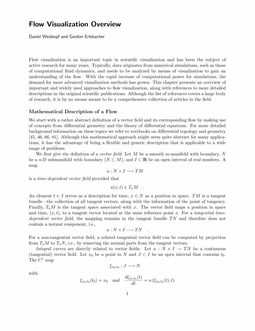
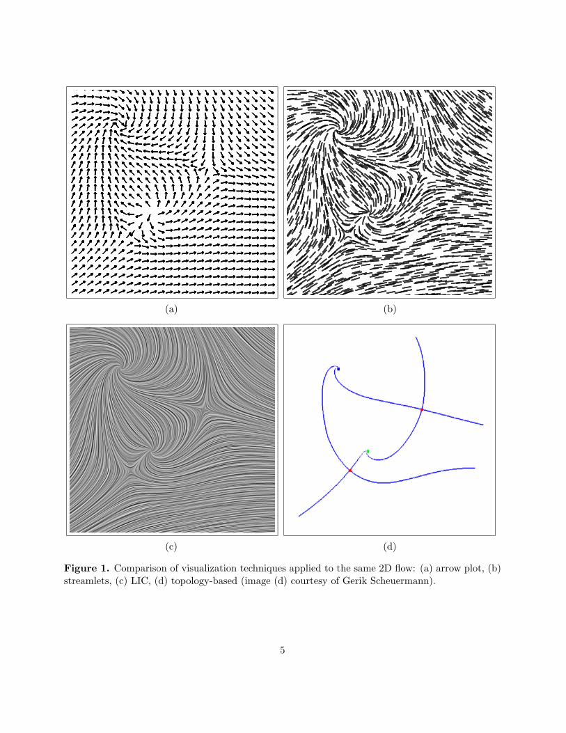
The traditional technique of arrow plots is a well-known example for direct flow visualization basedon glyphs. Small arrows are drawn at discrete grid points, showing the direction of the flow andserving as local probes for the velocity field; see Figure 1 (a). In the closely related hedgehogapproach, the flow is visualized by directed line segments whose lengths represent the magnitude ofthe velocity. To avoid possible distracting patterns for a uniform sampling by arrows or hedgehogs,randomness can be introduced in their positions [29]. Arrow plots can be directly applied to time-dependent vector fields by letting the arrows adapt to the velocity field for the current time. For 3Drepresentations, the following issues have to be considered: the position and orientation of an arrowis more difficult to understand due to the projection onto the 2D image plane, and an arrow mightocclude other arrows in the background. The problem of clutter can be addressed by highlightingarrows with orientations in a range specified by the user [9], or by selectively seeding the arrows.Illumination and shadows serve to improve spatial perception; for example, shadowing can be appliedto hedgehog visualizations on 2D slices of a 3D flow [65].

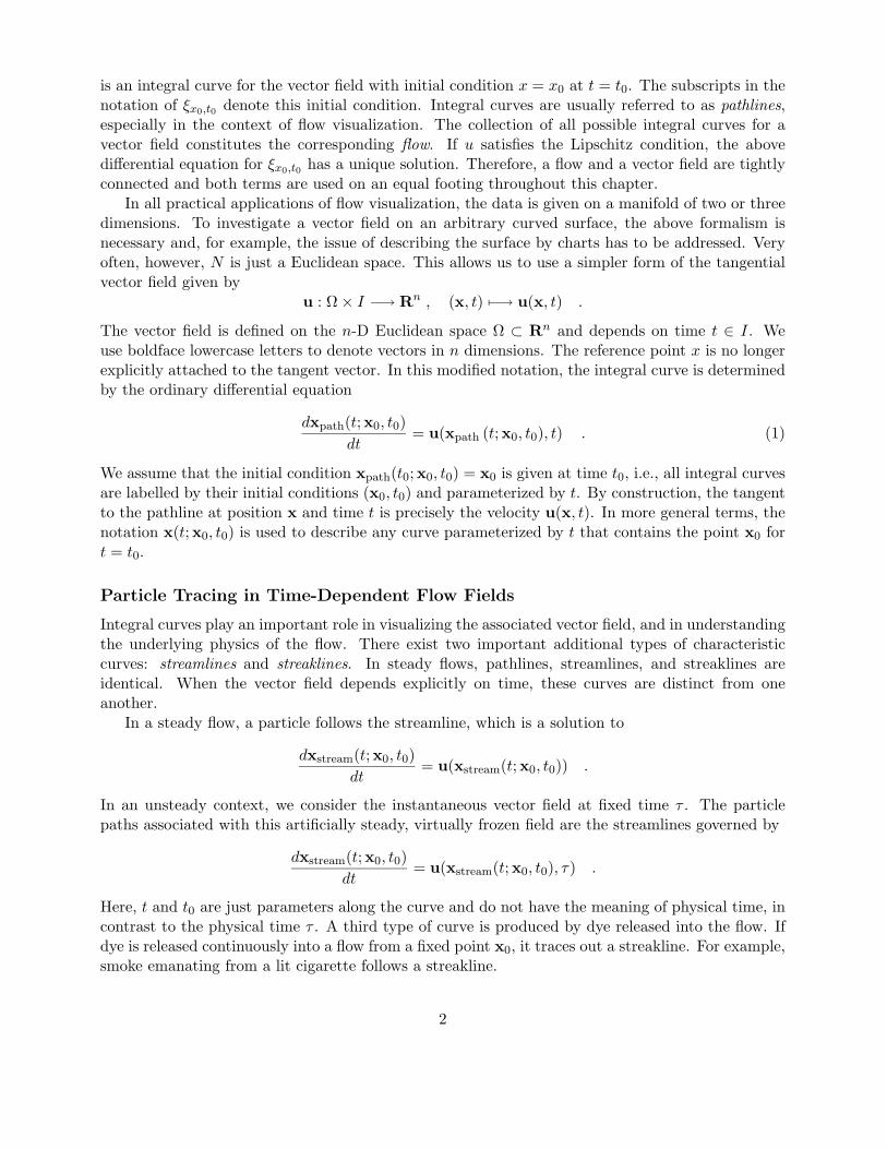
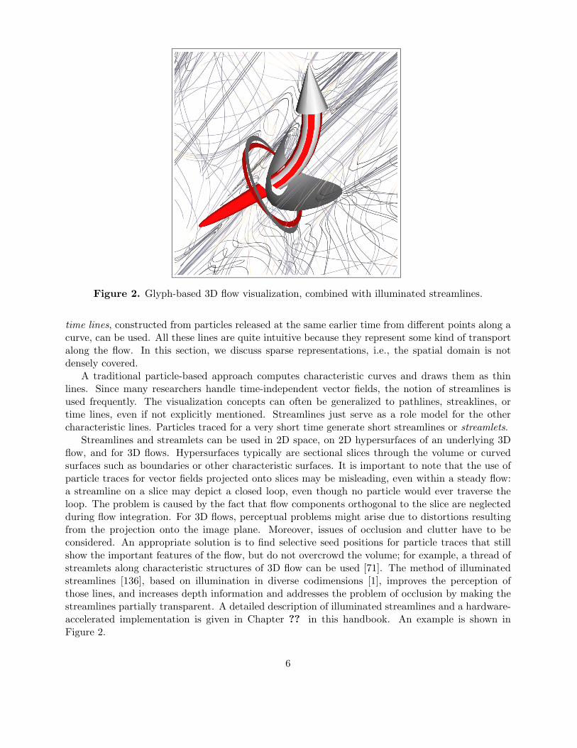
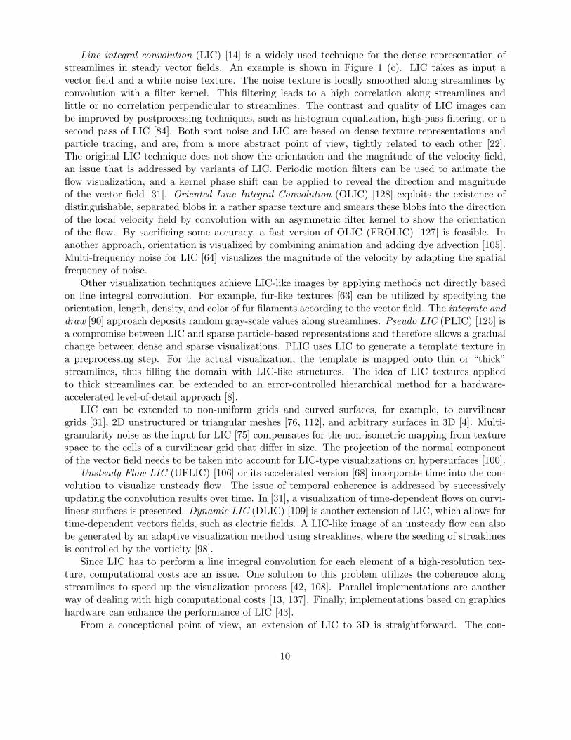
More complex glyphs [26] can be used to provide additional information on the flow at a pointof the flow; see Figure 2. In addition to the actual velocity, information on the Jacobian of thevelocity field is revealed. The Jacobian is presented in an intuitive way by decomposing the Jacobianmatrix into meaningful components and by mapping them to icons based on easily understandablemetaphors. Typical data encoded into glyphs comprises velocity, acceleration, curvature, localrotation, shear, or convergence. Glyphs can also be used to represent information on the uncertaintyof the vector field data [134]. Glyph-based uncertainty visualization is also covered in [69, 86], whichadditionally discuss uncertainty representations for other visualization styles.

Another strategy is to map flow properties to a single value and apply techniques known fromthe visualization of scalar data. Typically, the magnitude of the velocity or one of the velocitycomponents are used. For 2D flow visualization, a mapping to color or to isolines (contour lines)is often applied. Volume visualization techniques have to be employed in the case of 3D data.Direct volume rendering, which avoids occlusion problems by selective use of semi-transparency, canbe applied to single-component data derived from vector fields [30, 120]; recent developments arespecifically designed for time-dependent data [16, 36, 85].

Sparse Representations for Particle-Tracing Techniques

Another class of visualization approaches is based on the characteristic lines obtained by particletracing. Among these are the aforementioned pathlines, streamlines, and streaklines. In addition,

4

(a) (b)

(c) (d)

Figure 1. Comparison of visualization techniques applied to the same 2D flow: (a) arrow plot, (b)streamlets, (c) LIC, (d) topology-based (image (d) courtesy of Gerik Scheuermann).

5

Figure 2. Glyph-based 3D flow visualization, combined with illuminated streamlines.

time lines, constructed from particles released at the same earlier time from different points along acurve, can be used. All these lines are quite intuitive because they represent some kind of transportalong the flow. In this section, we discuss sparse representations, i.e., the spatial domain is notdensely covered.

A traditional particle-based approach computes characteristic curves and draws them as thinlines. Since many researchers handle time-independent vector fields, the notion of streamlines isused frequently. The visualization concepts can often be generalized to pathlines, streaklines, ortime lines, even if not explicitly mentioned. Streamlines just serve as a role model for the othercharacteristic lines. Particles traced for a very short time generate short streamlines or streamlets.

Streamlines and streamlets can be used in 2D space, on 2D hypersurfaces of an underlying 3Dflow, and for 3D flows. Hypersurfaces typically are sectional slices through the volume or curvedsurfaces such as boundaries or other characteristic surfaces. It is important to note that the use ofparticle traces for vector fields projected onto slices may be misleading, even within a steady flow:a streamline on a slice may depict a closed loop, even though no particle would ever traverse theloop. The problem is caused by the fact that flow components orthogonal to the slice are neglectedduring flow integration. For 3D flows, perceptual problems might arise due to distortions resultingfrom the projection onto the image plane. Moreover, issues of occlusion and clutter have to beconsidered. An appropriate solution is to find selective seed positions for particle traces that stillshow the important features of the flow, but do not overcrowd the volume; for example, a thread ofstreamlets along characteristic structures of 3D flow can be used [71]. The method of illuminatedstreamlines [136], based on illumination in diverse codimensions [1], improves the perception ofthose lines, and increases depth information and addresses the problem of occlusion by making thestreamlines partially transparent. A detailed description of illuminated streamlines and a hardware-accelerated implementation is given in Chapter ?? in this handbook. An example is shown inFigure 2.

6

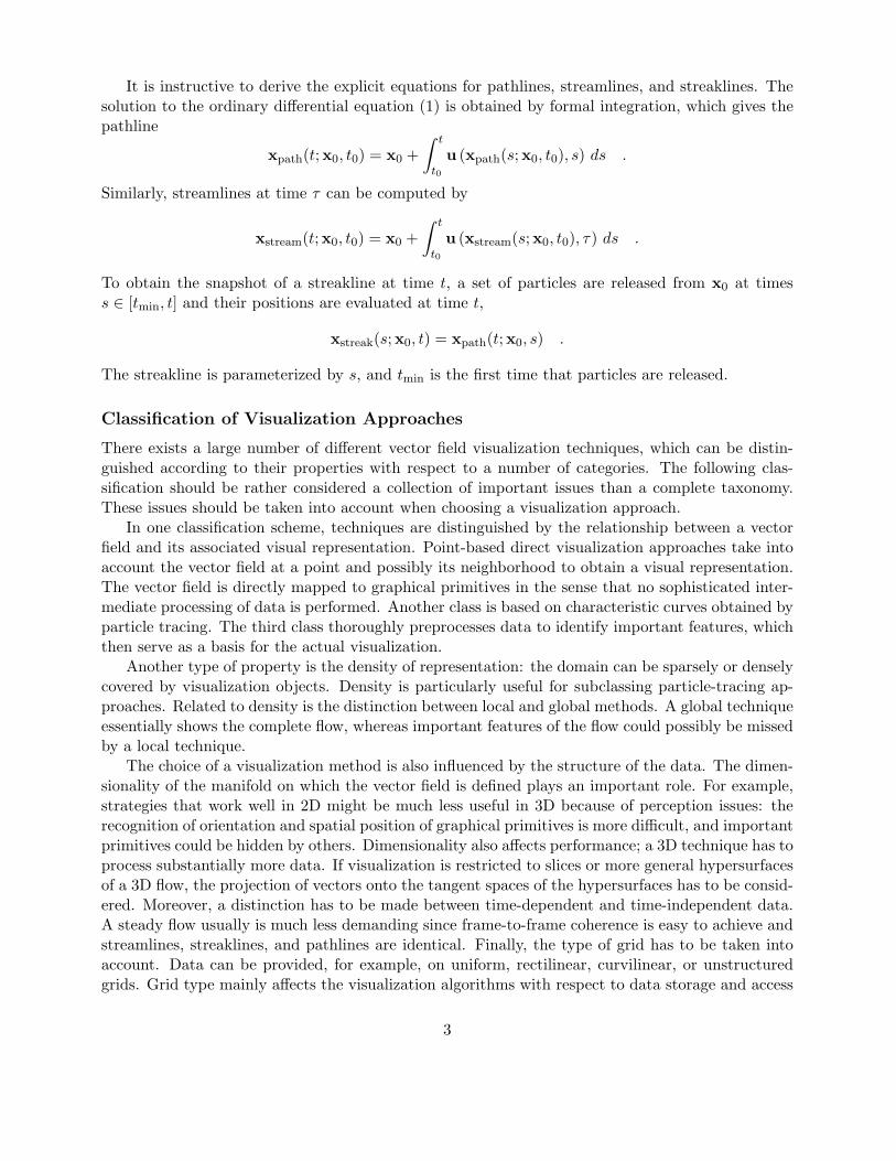
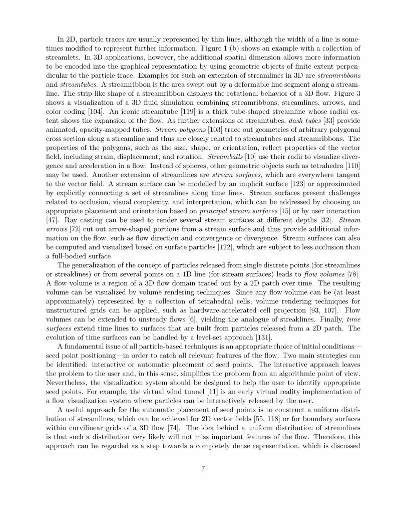
In 2D, particle traces are usually represented by thin lines, although the width of a line is some-times modified to represent further information. Figure 1 (b) shows an example with a collection ofstreamlets. In 3D applications, however, the additional spatial dimension allows more informationto be encoded into the graphical representation by using geometric objects of finite extent perpen-dicular to the particle trace. Examples for such an extension of streamlines in 3D are streamribbonsand streamtubes. A streamribbon is the area swept out by a deformable line segment along a stream-line. The strip-like shape of a streamribbon displays the rotational behavior of a 3D flow. Figure 3shows a visualization of a 3D fluid simulation combining streamribbons, streamlines, arrows, andcolor coding [104]. An iconic streamtube [119] is a thick tube-shaped streamline whose radial ex-tent shows the expansion of the flow. As further extensions of streamtubes, dash tubes [33] provideanimated, opacity-mapped tubes. Stream polygons [103] trace out geometries of arbitrary polygonalcross section along a streamline and thus are closely related to streamtubes and streamribbons. Theproperties of the polygons, such as the size, shape, or orientation, reflect properties of the vectorfield, including strain, displacement, and rotation. Streamballs [10] use their radii to visualize diver-gence and acceleration in a flow. Instead of spheres, other geometric objects such as tetrahedra [110]may be used. Another extension of streamlines are stream surfaces, which are everywhere tangentto the vector field. A stream surface can be modelled by an implicit surface [123] or approximatedby explicitly connecting a set of streamlines along time lines. Stream surfaces present challengesrelated to occlusion, visual complexity, and interpretation, which can be addressed by choosing anappropriate placement and orientation based on principal stream surfaces [15] or by user interaction[47]. Ray casting can be used to render several stream surfaces at different depths [32]. Streamarrows [72] cut out arrow-shaped portions from a stream surface and thus provide additional infor-mation on the flow, such as flow direction and convergence or divergence. Stream surfaces can alsobe computed and visualized based on surface particles [122], which are subject to less occlusion thana full-bodied surface.

The generalization of the concept of particles released from single discrete points (for streamlinesor streaklines) or from several points on a 1D line (for stream surfaces) leads to flow volumes [78].A flow volume is a region of a 3D flow domain traced out by a 2D patch over time. The resultingvolume can be visualized by volume rendering techniques. Since any flow volume can be (at leastapproximately) represented by a collection of tetrahedral cells, volume rendering techniques forunstructured grids can be applied, such as hardware-accelerated cell projection [93, 107]. Flowvolumes can be extended to unsteady flows [6], yielding the analogue of streaklines. Finally, timesurfaces extend time lines to surfaces that are built from particles released from a 2D patch. Theevolution of time surfaces can be handled by a level-set approach [131].

A fundamental issue of all particle-based techniques is an appropriate choice of initial conditions—seed point positioning—in order to catch all relevant features of the flow. Two main strategies canbe identified: interactive or automatic placement of seed points. The interactive approach leavesthe problem to the user and, in this sense, simplifies the problem from an algorithmic point of view.Nevertheless, the visualization system should be designed to help the user to identify appropriateseed points. For example, the virtual wind tunnel [11] is an early virtual reality implementation ofa flow visualization system where particles can be interactively released by the user.

A useful approach for the automatic placement of seed points is to construct a uniform distri-bution of streamlines, which can be achieved for 2D vector fields [55, 118] or for boundary surfaceswithin curvilinear grids of a 3D flow [74]. The idea behind a uniform distribution of streamlinesis that such a distribution very likely will not miss important features of the flow. Therefore, thisapproach can be regarded as a step towards a completely dense representation, which is discussed

7

Figure 3. Combination of streamlines, streamribbons, arrows, and color coding for a 3D flow(courtesy of BMW Group and Martin Schulz).

8

in the following section. Equally spaced streamlines can be extended to multiresolution hierarchiesthat support an interactive change of streamline density, while zooming in and out of the vectorfield [58]. Moreover, with this technique, the density of streamlines can be determined by propertiesof the flow, such as the magnitude of the velocity or the vorticity. Evenly spaced streamlines for anunsteady flow can be realized by correlating instantaneous streamline visualizations for subsequenttime steps [57]. Seeding strategies may also be based on vector field topology; for example, flowstructures in the vicinity of critical points can be visualized by appropriately setting the initialconditions for particle tracing [126].

Since all particle-tracing techniques are based on solving the differential equation for particletransport, issues of numerical accuracy and speed must be addressed. Different numerical tech-niques known from the literature can be applied for the initial value problem of ordinary differentialequations. In many applications, explicit integration schemes are used, such as non-adaptive oradaptive Runge-Kutta methods. The required accuracy for particle tracing depends on the visual-ization technique; for example, first order Euler integration might be acceptable for streamlets butnot for longer streamlines. A comparison of different integration schemes [111] helps to judge thetrade-off between computation time and accuracy. Besides the actual integration scheme, the gridon which the vector field is given is very important for choosing a particle-tracing technique. Pointlocation and interpolation heavily depend on the grid and therefore affect the speed and accuracyof particle tracing. Both aspects are detailed in [82], along with a comparision between C-space(computational space) and P-space (physical space) approaches. The numerics of particle tracingis discussed, for example, for tetrahedral decomposition of curvilinear grids [62], especially for thedecomposition of distorted cells [94], for unstructured grids [119], for analytical solutions in piece-wise linearly interpolated tetrahedral grids [83], for stiff differential equations originating from shearflows [111], and for sparse grids [113].

Dense Representations for Particle-Tracing Methods

Another class of visualization approaches is based on a representation of the flow by a dense coveragethrough structures determined by particle tracing. Typically, dense representations are built upontexture-based techniques, which provide images of high spatial resolution. A detailed descriptionof texture-based flow visualization and, in particular, its support by graphics hardware is discussedin Chapter ?? on “Flow Textures” in this handbook. A summary of research in the field of denserepresentations can be found in the survey [99].

The distinction between dense and sparse techniques should not be taken too rigidly becauseboth classes of techniques are closely related by the fact that they form visual structures basedon particle tracing. Therefore, dense representations also lead to the same intuitive understandingof the flow. Often, a transition between both classes is possible [125]; for example, texture-basedtechniques with only few distinct visual elements might resemble a collection of few streamlines and,on the other hand, evenly spaced streamline seeding can be used with a high density of lines.

An early texture-synthesis technique for vector field visualization is spot noise [121], whichproduces a texture by generating a set of spots on the spatial domain. Each spot represents aparticle moving over a short period of time and results in a streak in the direction of the flow at theposition of the spot. Enhanced spot noise [27] adds the visualization of the velocity magnitude andallows for curved spots. Spot noise can also be applied on boundaries and surfaces [20, 114]. A divide-and-conquer strategy makes possible an implementation of spot noise for interactive environments[19]. As an example application, spot noise was applied to the visualization of turbulent flow [21].

9

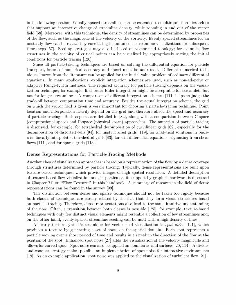
Line integral convolution (LIC) [14] is a widely used technique for the dense representation ofstreamlines in steady vector fields. An example is shown in Figure 1 (c). LIC takes as input avector field and a white noise texture. The noise texture is locally smoothed along streamlines byconvolution with a filter kernel. This filtering leads to a high correlation along streamlines andlittle or no correlation perpendicular to streamlines. The contrast and quality of LIC images canbe improved by postprocessing techniques, such as histogram equalization, high-pass filtering, or asecond pass of LIC [84]. Both spot noise and LIC are based on dense texture representations andparticle tracing, and are, from a more abstract point of view, tightly related to each other [22].The original LIC technique does not show the orientation and the magnitude of the velocity field,an issue that is addressed by variants of LIC. Periodic motion filters can be used to animate theflow visualization, and a kernel phase shift can be applied to reveal the direction and magnitudeof the vector field [31]. Oriented Line Integral Convolution (OLIC) [128] exploits the existence ofdistinguishable, separated blobs in a rather sparse texture and smears these blobs into the directionof the local velocity field by convolution with an asymmetric filter kernel to show the orientationof the flow. By sacrificing some accuracy, a fast version of OLIC (FROLIC) [127] is feasible. Inanother approach, orientation is visualized by combining animation and adding dye advection [105].Multi-frequency noise for LIC [64] visualizes the magnitude of the velocity by adapting the spatialfrequency of noise.

Other visualization techniques achieve LIC-like images by applying methods not directly basedon line integral convolution. For example, fur-like textures [63] can be utilized by specifying theorientation, length, density, and color of fur filaments according to the vector field. The integrate anddraw [90] approach deposits random gray-scale values along streamlines. Pseudo LIC (PLIC) [125] isa compromise between LIC and sparse particle-based representations and therefore allows a gradualchange between dense and sparse visualizations. PLIC uses LIC to generate a template texture ina preprocessing step. For the actual visualization, the template is mapped onto thin or “thick”streamlines, thus filling the domain with LIC-like structures. The idea of LIC textures appliedto thick streamlines can be extended to an error-controlled hierarchical method for a hardware-accelerated level-of-detail approach [8].

LIC can be extended to non-uniform grids and curved surfaces, for example, to curvilineargrids [31], 2D unstructured or triangular meshes [76, 112], and arbitrary surfaces in 3D [4]. Multi-granularity noise as the input for LIC [75] compensates for the non-isometric mapping from texturespace to the cells of a curvilinear grid that differ in size. The projection of the normal componentof the vector field needs to be taken into account for LIC-type visualizations on hypersurfaces [100].

Unsteady Flow LIC (UFLIC) [106] or its accelerated version [68] incorporate time into the con-volution to visualize unsteady flow. The issue of temporal coherence is addressed by successivelyupdating the convolution results over time. In [31], a visualization of time-dependent flows on curvi-linear surfaces is presented. Dynamic LIC (DLIC) [109] is another extension of LIC, which allows fortime-dependent vectors fields, such as electric fields. A LIC-like image of an unsteady flow can alsobe generated by an adaptive visualization method using streaklines, where the seeding of streaklinesis controlled by the vorticity [98].

Since LIC has to perform a line integral convolution for each element of a high-resolution tex-ture, computational costs are an issue. One solution to this problem utilizes the coherence alongstreamlines to speed up the visualization process [42, 108]. Parallel implementations are anotherway of dealing with high computational costs [13, 137]. Finally, implementations based on graphicshardware can enhance the performance of LIC [43].

From a conceptional point of view, an extension of LIC to 3D is straightforward. The con-

10

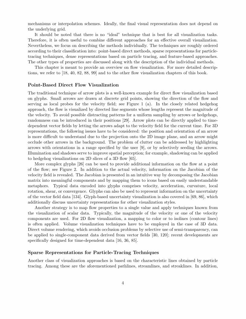
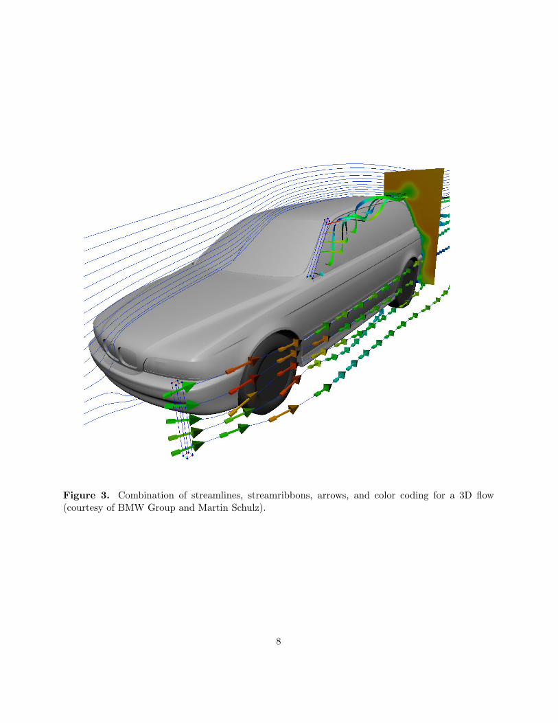
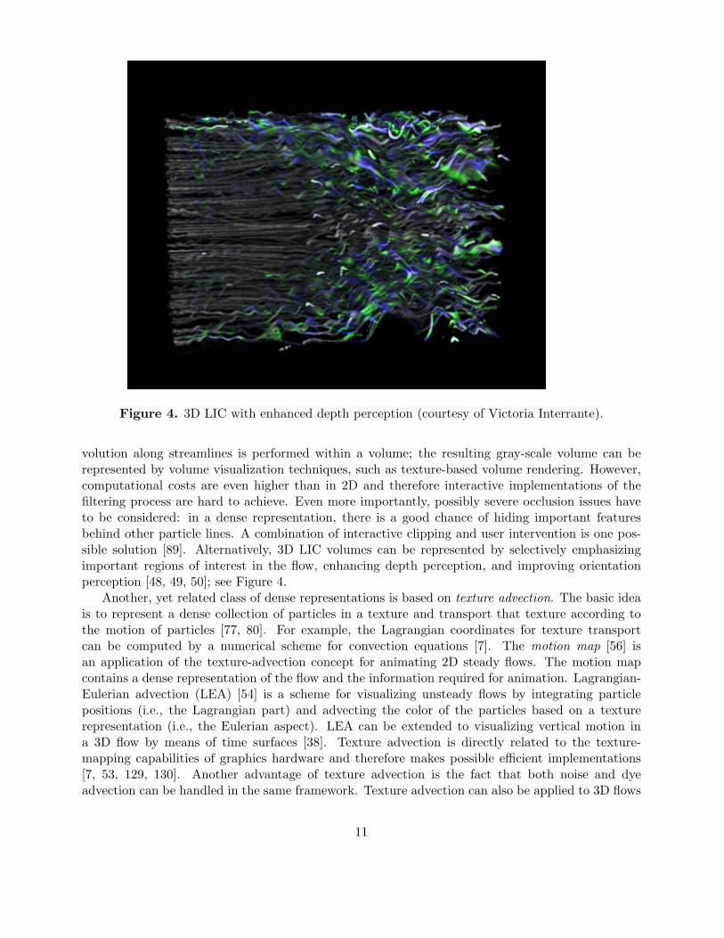
Figure 4. 3D LIC with enhanced depth perception (courtesy of Victoria Interrante).

volution along streamlines is performed within a volume; the resulting gray-scale volume can berepresented by volume visualization techniques, such as texture-based volume rendering. However,computational costs are even higher than in 2D and therefore interactive implementations of thefiltering process are hard to achieve. Even more importantly, possibly severe occlusion issues haveto be considered: in a dense representation, there is a good chance of hiding important featuresbehind other particle lines. A combination of interactive clipping and user intervention is one pos-sible solution [89]. Alternatively, 3D LIC volumes can be represented by selectively emphasizingimportant regions of interest in the flow, enhancing depth perception, and improving orientationperception [48, 49, 50]; see Figure 4.

Another, yet related class of dense representations is based on texture advection. The basic ideais to represent a dense collection of particles in a texture and transport that texture according tothe motion of particles [77, 80]. For example, the Lagrangian coordinates for texture transportcan be computed by a numerical scheme for convection equations [7]. The motion map [56] isan application of the texture-advection concept for animating 2D steady flows. The motion mapcontains a dense representation of the flow and the information required for animation. Lagrangian-Eulerian advection (LEA) [54] is a scheme for visualizing unsteady flows by integrating particlepositions (i.e., the Lagrangian part) and advecting the color of the particles based on a texturerepresentation (i.e., the Eulerian aspect). LEA can be extended to visualizing vertical motion ina 3D flow by means of time surfaces [38]. Texture advection is directly related to the texture-mapping capabilities of graphics hardware and therefore makes possible efficient implementations[7, 53, 129, 130]. Another advantage of texture advection is the fact that both noise and dyeadvection can be handled in the same framework. Texture advection can also be applied to 3D flows

11

[59, 130].Image based flow visualization (IBFV) [124] is a recently developed variant of 2D texture advec-

tion. Not only is the (noise) texture transported along the flow, but additionally a second textureis blended into the advected texture at each time step. IBFV is a flexible tool that can imitate awide variety of visualization styles. Another approach to the transport of a dense set of particles isbased on nonlinear diffusion [28]. An initial noise image is smoothed along integral lines of a steadyflow by diffusion, whereas the image is sharpened in the orthogonal direction. Nonlinear diffusioncan be extended to the multi-scale visualization of transport in time-dependent flows [12].

Finally, some 3D flow visualization techniques adopt the idea of splatting, originally developedfor volume rendering [132]. Even if some vector splatting techniques do not rely on particle tracing,we have included them in this section because their visual appearance resembles dense curve-likestructures. Anisotropic “scratches” can be modelled onto texture splats that are oriented along theflow to show the direction of the vector field [17]. Line bundles [79] use the splatting analogy todraw each data point with a pre-computed set of rendered line segments. These semitransparent linebundles are composited together in a back-to-front order to achieve an anisotropic volume renderingresult. For time-dependent flows, the animation of a large number of texture-mapped particles alongpathlines can be used [39]. For all splatting approaches, the density of representation depends onthe number of splats.

Feature-Based Visualization Approaches

The visualization concepts discussed so far operate directly on the vector field. Therefore, it is thetask of the user to identify the important features of the flow from such a visualization. Feature-basedvisualization approaches seek to compute a more abstract representation that already contains theimportant properties in a condensed form and suppresses superfluous information. In other words,an appropriate filtering process is chosen to reduce the amount of visual data presented to the user.Examples for this more abstract data are flow topology based on critical points, other flow featuressuch as vortices and shock waves, or aggregated flow data via clustering.

After features are computed, the actual visual representation has to be considered. Differentfeatures have different attributes; to emphasize special attributes for each type of feature, suitablerepresentations must be used. Glyphs or icons can be employed for vortices or for critical points andother topological features. One example are ellipses or ellipsoids to encode the rotation speed andother attributes of vortices. A comprehensive presentation of feature extraction and visualizationtechniques can be found in the survey [88].

Topology-based 2D vector field visualization [44] aims to show only the essential informationof the field. The qualitative structure of a vector field can be globally represented by portrayingits topology. The field’s critical points and separatrices completely determine the nature of theflow. From a diagram of the topology, the complete flow can be inferred. Figure 1 (d) showsan example of a topology-based visualization. From a numerical point of view, the interpolationscheme is crucial for identifying critical points. Extended versions of topology-based representationsmake use of higher-order singularities [101] and C1-continuous interpolation schemes [102]. Anotherextension is based on the detection of closed streamlines, a global property that is not detected bythe aforementioned algorithms [133]. Topology-based visualization can also be extended to time-dependent vector fields by topology tracking [117]. The original topology-based techniques workwell for data sets with a small number of critical points. Turbulent flows computed on a high-resolution grid, however, may show a large number of critical points, leading to an overloaded visual

12

representation. This issue is addressed by topology simplification techniques [23, 24, 25, 115, 116],which remove some of the critical points and leave only the important features. For the visualizationof 3D topology, appropriate visual representations need to be used. For example, streamlines thatare traced from appropriate positions close to critical points connect to other critical points or theboundary to display the topology, while glyphs can be used to visualize the various classes of criticalpoints [37]. Topology can also serve as a means for determining the similarity between two differentvector fields [3, 67].

Vector field clustering is another way to reduce the amount of visualization data. A large numberof vectors of the original high-resolution field are combined into fewer vectors that approximatelyrepresent the vector field at a coarser resolution, leading to a visualization of aggregated data. Animportant issue is to establish appropriate error measures to control the way vectors are combinedinto clusters [70, 114]. The extension of vector field clustering to several levels of clustering leads tohierarchical representations [34, 35, 41]. Vector field clustering can not only be applied to 2D and 3Dflows, but also on 2D slices [135]. In related approaches, segmentation [28], multi-scale visualization[12], or topology-preserving smoothing based on level-set techniques [131] reduce the complexity ofthe displayed vector fields.

An important class of feature detection algorithms is based on the identification of vortices andtheir respective vortex cores. Vortices are useful for identifying significant features in a fluid flow.One way of classifying vortex detection techniques is the distinction between point-based, localtechniques, which directly operate on the vector data set, and geometry-based, global techniques,which examine the properties of characteristic lines around vortices [97]. Local techniques build ameasure for vortices from physical quantities of a fluid flow. An overview on these techniques is givenin [2, 91]; more recent contributions are presented in [5, 52, 61, 92]. A mathematical framework [87]makes it possible to unify several vortex detection methods. Point-based methods are rather simpleto compute, but are more likely to miss some vortices. For example, weak vortices, which have a slowrotational component compared to the velocity of the core, are hard to detect by these techniques.Geometry-based, global methods [51, 95, 96] are usually associated with higher computational costs,but allow a more robust detection or verification of vortices. A more detailed description of vortexdetection techniques can be found in Chapter ?? on “Detection and Visualization of Vortices” inthis handbook.

Shock waves are another important feature of a fluid flow because they can increase drag andeven cause structural failure. Shock waves are characterized by discontinuities in physical quantities,such as pressure, density, and velocity. Therefore, shock detection algorithms are related to edgedetection methods known from image processing. A comparison of different techniques for shockextraction and visualization can be found in [73]. Flow separation and attachment, which occurwhen a flow abruptly moves away from, or returns to, a solid body, are another interesting featureof a fluid flow. Attachment and separation lines on surfaces in a 3D flow can be automaticallyextracted based on a local analysis of the vector field by means phase plane analysis [60].

Vortex cores, shock waves, and separation and attachment lines are examples of features that aretightly connected to an underlying physical model and cannot be derived from a generic vector fielddescription. Therefore, a profound understanding of the physical problem is necessary to developmeasures for these kinds of features. Accordingly, a large body of research on feature extractioncan be found in the literature on related topics of engineering and physics. Since a comprehensivecollection of techniques and references on feature extraction is beyond the scope of this chapter, werefer to the survey [88] for more detailed information.

13

Acknowledgments

We would like to thank the following people for providing us with images: Victoria Interrante(University of Minnesota) for the image in Figure 4; Gerik Scheuermann (Universitat Kaiserslautern)for Figure 1 (d); BMW Group and Martin Schulz (science + computing) for Figure 3.

The first author thanks Landesstiftung Baden-Wurttemberg for support, the second authoracknowledges support from NSF under grant NSF-0083792.

References

[1] D. C. Banks. Illumination in diverse codimensions. In Proceedings of ACM SIGGRAPH 94,pages 327–334, 1994.

[2] D. C. Banks and B. A. Singer. Vortex tubes in turbulent flows: Identification, representation,reconstruction. In IEEE Visualization ’94, pages 132–139, 1994.

[3] R. K. Batra and L. Hesselink. Feature comparisons of 3-D vector fields using Earth mover’sdistance. In IEEE Visualization ’99, pages 105–114, 1999.

[4] H. Battke, D. Stalling, and H.-C. Hege. Fast line integral convolution for arbitrary surfacesin 3D. In H.-C. Hege and K. Polthier, editors, Mathematical Visualization, pages 181–195.Springer, 1997.

[5] D. Bauer and R. Peikert. Vortex tracking in scale-space. In EG / IEEE TCVG Symposiumon Visualization ’02, pages 233–240, 2002.

[6] B. Becker, D. A. Lane, and N. Max. Unsteady flow volumes. In IEEE Visualization ’95, pages329–335, 1995.

[7] J. Becker and M. Rumpf. Visualization of time-dependent velocity fields by texture transport.In EG Workshop on Visualization in Scientific Computing, pages 91–102, 1998.

[8] U. Bordoloi and H.-W. Shen. Hardware accelerated interactive vector field visualization: Alevel of detail approach. In Eurographics ’02, pages 605–614, 2002.

[9] E. Boring and A. Pang. Directional flow visualization of vector fields. In IEEE Visualization’96, pages 389–392, 1996.

[10] M. Brill, H. Hagen, H.-C. Rodrian, W. Djatschin, and S. V. Klimenko. Streamball techniquesfor flow vizualization. In IEEE Visualization ’94, pages 225–231, 1994.

[11] S. Bryson and C. Levit. The virtual wind tunnel. IEEE Computer Graphics and Applications,12(4):25–34, 1992.

[12] D. Burkle, T. Preußer, and M. Rumpf. Transport and anisotropic diffusion in time-dependentflow visualization. In IEEE Visualization ’01, pages 61–67, 2001.

[13] B. Cabral and C. Leedom. Highly parallel vector visualization using line integral convolution.In SIAM Conference on Parallel Processing for Scientific Computing, pages 802–807, 1995.

[14] B. Cabral and L. C. Leedom. Imaging vector fields using line integral convolution. In Pro-ceedings of ACM SIGGRAPH 93, pages 263–272, 1993.

14

[15] W. Cai and P.-A. Heng. Principal stream surfaces. In IEEE Visualization ’97, pages 75–80,1997.

[16] J. Clyne and J. Dennis. Interactive direct volume rendering of time-varying data. In EG /IEEE TCVG Symposium on Visualization ’99, pages 109–120, 1999.

[17] R. Crawfis and N. Max. Texture splats for 3D scalar and vector field visualization. In IEEEVisualization ’93, pages 261–267, 1993.

[18] R. Crawfis, H.-W. Shen, and N. Max. Flow visualization techniques for CFD using volumerendering. In 9th International Symposium on Flow Visualization, pages 64/1–64/10, 2000.

[19] W. C. de Leeuw. Divide and conquer spot noise. In Supercomputing ’97 Conference, pages12–24, 1997.

[20] W. C. de Leeuw and H.-G. Pagendarm. Visual simulation of experimental oil-flow visualizationby spot noise images from numerical flow simulation. In EG Workshop on Visualization inScientific Computing, pages 135–148, 1995.

[21] W. C. de Leeuw, F. H. Post, and R. W. Vaatstra. Visualization of turbulent flow by spot noise.In EG Workshop on Virtual Environments and Scientific Visualization ’96, pages 287–295,1996.

[22] W. C. de Leeuw and R. van Liere. Comparing LIC and spot noise. In IEEE Visualization ’98,pages 359–366, 1998.

[23] W. C. de Leeuw and R. van Liere. Collapsing flow topology using area metrics. In IEEEVisualization ’99, pages 349–354, 1999.

[24] W. C. de Leeuw and R. van Liere. Visualization of global flow structures using multiple levelsof topology. In EG / IEEE TCVG Symposium on Visualization ’99, pages 45–52, 1999.

[25] W. C. de Leeuw and R. van Liere. Multi-level topology for flow visualization. Computers andGraphics, 24(3):325–331, 2000.

[26] W. C. de Leeuw and J. J. van Wijk. A probe for local flow field visualization. In IEEEVisualization ’93, pages 39–45, 1993.

[27] W. C. de Leeuw and J. J. van Wijk. Enhanced spot noise for vector field visualization. InIEEE Visualization ’95, pages 233–239, 1995.

[28] U. Diewald, T. Preußer, and M. Rumpf. Anisotropic diffusion in vector field visualization onEuclidean domains and surfaces. IEEE Transactions on Visualization and Computer Graphics,6(2):139–149, 2000.

[29] D. Dovey. Vector plots for irregular grids. In IEEE Visualization ’95, pages 248–253, 1995.

[30] D. S. Ebert, R. Yagel, J. Scott, and Y. Kurzion. Volume rendering methods for computationalfluid dynamics visualization. In IEEE Visualization ’94, pages 232–239, 1994.

15

[31] L. K. Forssell and S. D. Cohen. Using line integral convolution for flow visualization: Curvilin-ear grids, variable-speed animation, and unsteady flows. IEEE Transactions on Visualizationand Computer Graphics, 1(2):133–141, 1995.

[32] T. Fruhauf. Raycasting vector fields. In IEEE Visualization ’96, pages 115–120, 1996.

[33] A. Fuhrmann and E. Groller. Real-time techniques for 3D flow visualization. In IEEE Visu-alization ’98, pages 305–312, 1998.

[34] H. Garcke, T. Preußer, M. Rumpf, A. Telea, U. Weikard, and J. J. van Wijk. A phase fieldmodel for continuous clustering on vector fields. IEEE Transactions on Visualization andComputer Graphics, 7(3):230–241, 2001.

[35] H. Garcke, T. Preußer, M. Rumpf, A. Telea, U. Weikard, and J. V. Wijk. A continuousclustering method for vector fields. In IEEE Visualization ’00, pages 351–358, 2000.

[36] T. Glau. Exploring instationary fluid flows by interactive volume movies. In EG / IEEETCVG Symposium on Visualization ’99, pages 277–283. 1999.

[37] A. Globus, C. Levit, and T. Lasinski. A tool for visualizing the topology of three-dimensionalvector fields. In IEEE Visualization ’91, pages 33–40, 1991.

[38] J. Grant, G. Erlebacher, and J. O’Brien. Case study: Visualization of thermoclines in theocean using Lagrangian-Eulerian time surfaces. In IEEE Visualization ’02, pages 529–532,2002.

[39] S. Guthe, S. Gumhold, and W. Straßer. Interactive visualization of volumetric vector fieldsusing texture based particles. In WSCG 2002 Conference Proceedings, pages 33–41, 2002.

[40] H. Hauser, R. S. Laramee, and H. Doleisch. State-of-the-art report 2002 in flow visualization.TR-VRVis-2002-003, VRVis Research Center, Feb. 2002.

[41] B. Heckel, G. H. Weber, B. Hamann, and K. I. Joy. Construction of vector field hierarchies.In IEEE Visualization ’99, pages 19–26, 1999.

[42] H.-C. Hege and D. Stalling. Fast LIC with piecewise polynomial filter kernels. In H.-C. Hegeand K. Polthier, editors, Mathematical Visualization, pages 295–314. Springer, 1998.

[43] W. Heidrich, R. Westermann, H.-P. Seidel, and T. Ertl. Applications of pixel textures invisualization and realistic image synthesis. In ACM Symposium on Interactive 3D Graphics,pages 127–134, 1999.

[44] J. Helman and L. Hesselink. Representation and display of vector field topology in fluid flowdata sets. Computer, 22(8):27–36, 1989.

[45] M. W. Hirsch. Differential Topology. Springer, Berlin, 6th edition, 1997.

[46] M. W. Hirsch and S. Smale. Differential Equations, Dynamical Systems, and Linear Algebra.Academic Press, New York, 1974.

[47] J. P. M. Hultquist. Interactive numerical flow visualization using stream surfaces. ComputingSystems in Engineering, 1(2-4):349–353, 1990.

16

[48] V. Interrante. Illustrating surface shape in volume data via principal direction-driven 3D lineintegral convolution. In Proceedings of ACM SIGGRAPH 97, pages 109–116, 1997.

[49] V. Interrante and C. Grosch. Strategies for effectively visualizing 3D flow with volume LIC.In IEEE Visualization ’97, pages 421–424, 1997.

[50] V. Interrante and C. Grosch. Visualizing 3D flow. IEEE Computer Graphics and Applications,18(4):49–53, 1998.

[51] M. Jiang, R. Machiraju, and D. Thompson. Geometric verification of swirling features in flowfields. In IEEE Visualization ’02, pages 307–314, 2002.

[52] M. Jiang, R. Machiraju, and D. Thompson. A novel approach to vortex core region detection.In EG / IEEE TCVG Symposium on Visualization ’02, pages 217–232, 2002.

[53] B. Jobard, G. Erlebacher, and M. Y. Hussaini. Hardware-accelerated texture advection forunsteady flow visualization. In IEEE Visualization ’00, pages 155–162, 2000.

[54] B. Jobard, G. Erlebacher, and M. Y. Hussaini. Lagrangian-Eulerian advection for unsteadyflow visualization. In IEEE Visualization ’01, pages 53–60, 2001.

[55] B. Jobard and W. Lefer. Creating evenly-spaced streamlines of arbitrary density. In EGWorkshop on Visualization in Scientific Computing, pages 43–56, 1997.

[56] B. Jobard and W. Lefer. The motion map: Efficient computation of steady flow animations.In IEEE Visualization ’97, pages 323–328, 1997.

[57] B. Jobard and W. Lefer. Unsteady flow visualization by animating evenly-spaced streamlines.In Eurographics ’00, pages 31–40, 2000.

[58] B. Jobard and W. Lefer. Multiresolution flow visualization. In WSCG 2001 ConferenceProceedings, pages P34–P37, 2001.

[59] D. Kao, B. Zhang, K. Kim, and A. Pang. 3D flow visualization using texture advection. InIASTED Conference on Computer Graphics and Imaging 01 (CGMI), pages 252–257, 2001.

[60] D. N. Kenwright. Automatic detection of open and closed separation and attachment lines.In IEEE Visualization ’98, pages 151–158, 1998.

[61] D. N. Kenwright and R. Haimes. Automatic vortex core detection. IEEE Computer Graphicsand Applications, 18(4):70–74, 1998.

[62] D. N. Kenwright and D. A. Lane. Interactive time-dependent particle tracing using tetrahedraldecomposition. IEEE Transactions on Visualization and Computer Graphics, 2(2):120–129,1996.

[63] L. Khouas, C. Odet, and D. Friboulet. 2D vector field visualization using furlike texture. InEG / IEEE TCVG Symposium on Visualization ’99, pages 35–44. 1999.

[64] M.-H. Kiu and D. C. Banks. Multi-frequency noise for LIC. In IEEE Visualization ’96, pages121–126, 1996.

17

[65] R. V. Klassen and S. J. Harrington. Shadowed hedgehogs: A technique for visualizing 2Dslices of 3D vector fields. In IEEE Visualization ’91, pages 148–153, 1991.

[66] S. Lang. Differential and Riemannian Manifolds. Springer, New York, 3rd edition, 1995.

[67] Y. Lavin, R. Batra, and L. Hesselink. Feature comparisons of vector fields using Earth mover’sdistance. In IEEE Visualization ’98, pages 103–110, 1998.

[68] Z. P. Liu and R. J. Moorhead. AUFLIC: An accelerated algorithm for unsteady flow lineintegral convolution. In EG / IEEE TCVG Symposium on Visualization ’02, pages 43–52,2002.

[69] S. K. Lodha, A. Pang, R. E. Sheehan, and C. M. Wittenbrink. UFLOW: Visualizing uncer-tainty in fluid flow. In IEEE Visualization ’96, pages 249–254, 1996.

[70] S. K. Lodha, J. C. Renteria, and K. M. Roskin. Topology preserving compression of 2D vectorfields. In IEEE Visualization ’00, pages 343–350, 2000.

[71] H. Loffelmann and E. Groller. Enhancing the visualization of characteristic structures indynamical systems. In EG Workshop on Visualization in Scientific Computing, pages 59–68,1998.

[72] H. Loffelmann, L. Mroz, E. Groller, and W. Purgathofer. Stream arrows: Enhancing theuse of stream surfaces for the visualization of dynamical systems. The Visual Computer,13(8):359–369, 1997.

[73] K.-L. Ma, J. V. Rosendale, and W. Vermeer. 3D shock wave visualization on unstructuredgrids. In 1996 Volume Visualization Symposium, pages 87–96, 1996.

[74] X. Mao, Y. Hatanaka, H. Higashida, and A. Imamiya. Image-guided streamline placement oncurvilinear grid surfaces. In IEEE Visualization ’98, pages 135–142, 1998.

[75] X. Mao, L. Hong, A. Kaufman, N. Fujita, and M. Kikukawa. Multi-granularity noise forcurvilinear grid LIC. In Graphics Interface, pages 193–200, 1998.

[76] X. Mao, M. Kikukawa, N. Fujita, and A. Imamiya. Line integral convolution for 3D surfaces.In EG Workshop on Visualization in Scientific Computing, pages 57–70, 1997.

[77] N. Max and B. Becker. Flow visualization using moving textures. In Proceedings of theICASW/LaRC Symposium on Visualizing Time-Varying Data, pages 77–87, 1995.

[78] N. Max, B. Becker, and R. Crawfis. Flow volumes for interactive vector field visualization. InIEEE Visualization ’93, pages 19–24, 1993.

[79] N. Max, R. Crawfis, and C. Grant. Visualizing 3D velocity fields near contour surfaces. InIEEE Visualization ’94, pages 248–256, 1994.

[80] N. Max, R. Crawfis, and D. Williams. Visualizing wind velocities by advecting cloud textures.In IEEE Visualization ’92, pages 179–184, 1992.

[81] J. W. Milnor. Topology from the Differentiable Viewpoint. University Press of Virginia, Char-lottesville, 1965.

18

[82] G. M. Nielson, H. Hagen, and H. Muller. Scientific Visualization: Overviews, Methodologies,and Techniques. IEEE Computer Society Press, Silver Spring, MD, 1997.

[83] G. M. Nielson and I.-H. Jung. Tools for computing tangent curves for linearly varying vectorfields over tetrahedral domains. IEEE Transactions on Visualization and Computer Graphics,5(4):360–372, 1999.

[84] A. Okada and D. Kao. Enhanced line integral convolution with flow feature detection. InProceedings of IS&T/SPIE Electronic Imaging ’97, pages 206–217, 1997.

[85] K. Ono, H. Matsumoto, and R. Himeno. Visualization of thermal flows in an automotive cabinwith volume rendering method. In EG / IEEE TCVG Symposium on Visualization ’01, pages301–308, 2001.

[86] A. T. Pang, C. M. Wittenbrink, and S. K. Lodha. Approaches to uncertainty visualization.The Visual Computer, 13(8):370–390, 1997.

[87] R. Peikert and M. Roth. The ”parallel vectors” operator – a vector field visualization primitive.In IEEE Visualization ’99, pages 263–270, 1999.

[88] F. H. Post, B. Vrolijk, H. Hauser, R. S. Laramee, and H. Doleisch. Feature extraction andvisualization of flow fields. In Eurographics 2002 State-of-the-Art Reports, pages 69–100, 2002.

[89] C. Rezk-Salama, P. Hastreiter, C. Teitzel, and T. Ertl. Interactive exploration of volume lineintegral convolution based on 3D-texture mapping. In IEEE Visualization ’99, pages 233–240,1999.

[90] C. P. Risquet. Visualizing 2D flows: Integrate and draw. In EG Workshop on Visualizationin Scientific Computing, pages 132–142, 1998.

[91] M. Roth and R. Peikert. Flow visualization for turbomachinery design. In IEEE Visualization’96, pages 381–384, 1996.

[92] M. Roth and R. Peikert. A higher-order method for finding vortex core lines. In IEEEVisualization ’98, pages 143–150, 1998.

[93] S. Rottger, M. Kraus, and T. Ertl. Hardware-accelerated volume and isosurface renderingbased on cell-projection. In IEEE Visualization ’00, pages 109–116, 2000.

[94] I. A. Sadarjoen, A. J. de Boer, F. H. Post, and A. E. Mynett. Patricle tracing in σ-transformedgrids using tetrahedral 6-decomposition. In EG Workshop on Visualization in Scientific Com-puting, pages 71–80, 1998.

[95] I. A. Sadarjoen and F. H. Post. Geometric methods for vortex extraction. In EG / IEEETCVG Symposium on Visualization ’99, pages 53–62, 1999.

[96] I. A. Sadarjoen and F. H. Post. Detection, quantification, and tracking of vortices usingstreamline geometry. Computers and Graphics, 24(3):333–341, 2000.

[97] I. A. Sadarjoen, F. H. Post, B. Ma, D. C. Banks, and H.-G. Pagendarm. Selective visualizationof vortices in hydrodynamic flows. In IEEE Visualization ’98, pages 419–422, 1998.

19

[98] A. Sanna, B. Montrucchio, and R. Arina. Visualizing unsteady flows by adaptive streaklines.In WSCG 2000 Conference Proceedings, pages 84–91, 2000.

[99] A. Sanna, B. Montrucchio, and P. Montuschi. A survey on visualization of vector fields bytexture-based methods. Recent Res. Devel. Pattern Rec., 1:13–27, 2000.

[100] G. Scheuermann, H. Burbach, and H. Hagen. Visualizing planar vector fields with normalcomponent using line integral convolution. In IEEE Visualization ’99, pages 255–262, 1999.

[101] G. Scheuermann, H. Hagen, H. Kruger, M. Menzel, and A. P. Rockwood. Visualization ofhigher order singularities in vector fields. In IEEE Visualization ’97, pages 67–74, 1997.

[102] G. Scheuermann, X. Tricoche, and H. Hagen. C1-interpolation for vector field topology visu-alization. In IEEE Visualization ’99, pages 271–278, 1999.

[103] W. Schroeder, C. R. Volpe, and W. E. Lorensen. The stream polygon: A technique for 3Dvector field visualization. In IEEE Visualization ’91, pages 126–132, 1991.

[104] M. Schulz, F. Reck, W. Bartelheimer, and T. Ertl. Interactive visualization of fluid dynamicssimulations in locally refined Cartesian grids. In IEEE Visualization ’99, pages 413–416, 1999.

[105] H.-W. Shen, C. R. Johnson, and K.-L. Ma. Visualizing vector fields using line integral convo-lution and dye advection. In 1996 Volume Visualization Symposium, pages 63–70, 1996.

[106] H.-W. Shen and D. L. Kao. A new line integral convolution algorithm for visualizing time-varying flow fields. IEEE Transactions on Visualization and Computer Graphics, 4(2):98–108,1998.

[107] P. Shirley and A. Tuchman. A polygonal approximation to direct scalar volume rendering. InWorkshop on Volume Visualization ’90, pages 63–70, 1990.

[108] D. Stalling and H.-C. Hege. Fast and resolution independent line integral convolution. InProceedings of ACM SIGGRAPH 95, pages 249–256, 1995.

[109] A. Sundquist. Dynamic line integral convolution for visualizing streamline evolution. IEEETransactions on Visualization and Computer Graphics, 2003.

[110] C. Teitzel and T. Ertl. New approaches for particle tracing on sparse grids. In EG / IEEETCVG Symposium on Visualization ’99, pages 73–84, 1999.

[111] C. Teitzel, R. Grosso, and T. Ertl. Efficient and reliable integration methods for particletracing in unsteady flows on discrete meshes. In EG Workshop on Visualization in ScientificComputing, pages 49–56, 1997.

[112] C. Teitzel, R. Grosso, and T. Ertl. Line integral convolution on triangulated surfaces. InWSCG 1997 Conference Proceedings, pages 572–581, 1997.

[113] C. Teitzel, R. Grosso, and T. Ertl. Particle tracing on sparse grids. In EG Workshop onVisualization in Scientific Computing, pages 132–142, 1998.

[114] A. Telea and J. J. van Wijk. Simplified representation of vector fields. In IEEE Visualization’99, pages 35–42, 1999.

20

[115] X. Tricoche and G. Scheuermann. Continuous topology simplification of planar vector fields.In IEEE Visualization ’01, pages 159–166, 2001.

[116] X. Tricoche, G. Scheuermann, and H. Hagen. A topology simplification method for 2D vectorfields. In IEEE Visualization ’00, pages 359–366, 2000.

[117] X. Tricoche, T. Wischgoll, G. Scheuermann, and H. Hagen. Visualization of very large datasets:Topology tracking for the visualization of time-dependent two-dimensional flows. Computersand Graphics, 26(2):249–257, 2002.

[118] G. Turk and D. Banks. Image-guided streamline placement. In Proceedings of ACM SIG-GRAPH 96, pages 453–460, 1996.

[119] S.-K. Ueng, C. Sikorski, and K.-L. Ma. Efficient streamline, streamribbon, and streamtube con-structions on unstructured grids. IEEE Transactions on Visualization and Computer Graphics,2(2):100–110, 1996.

[120] S. P. Uselton. Volume rendering for computational fluid dynamics: Initial results. TechnicalReport RNR-91-026, NASA Ames Research Center, Sept. 1991.

[121] J. J. van Wijk. Spot noise – texture synthesis for data visualization. Computer Graphics(Proceedings of ACM SIGGRAPH 91), 25:309–318, 1991.

[122] J. J. van Wijk. Flow visualization with surface particles. IEEE Computer Graphics andApplications, 13(4):18–24, 1993.

[123] J. J. van Wijk. Implicit stream surfaces. In IEEE Visualization ’93, pages 245–252, 1993.

[124] J. J. van Wijk. Image based flow visualization. ACM Transactions on Graphics, 21(3):745–754,2002.

[125] V. Verma, D. Kao, and A. Pang. PLIC: Bridging the gap between streamlines and LIC. InIEEE Visualization ’99, pages 341–348, 1999.

[126] V. Verma, D. Kao, and A. Pang. A flow-guided streamline seeding strategy. In IEEE Visual-ization ’00, pages 163–170, 2000.

[127] R. Wegenkittl and E. Groller. Fast oriented line integral convolution for vector field visualiza-tion via the Internet. In IEEE Visualization ’97, pages 309–316, 1997.

[128] R. Wegenkittl, E. Groller, and W. Purgathofer. Animating flow fields: Rendering of orientedline integral convolution. In Computer Animation ’97, pages 15–21, 1997.

[129] D. Weiskopf, G. Erlebacher, M. Hopf, and T. Ertl. Hardware-accelerated Lagrangian-Euleriantexture advection for 2D flow visualization. In Vision, Modeling, and Visualization VMV ’02Conference, pages 77–84, 2002.

[130] D. Weiskopf, M. Hopf, and T. Ertl. Hardware-accelerated visualization of time-varying 2Dand 3D vector fields by texture advection via programmable per-pixel operations. In Vision,Modeling, and Visualization VMV ’01 Conference, pages 439–446, 2001.

21

[131] R. Westermann, C. Johnson, and T. Ertl. Topology-preserving smoothing of vector fields.IEEE Transactions on Visualization and Computer Graphics, 7(3):222–229, 2001.

[132] L. Westover. Footprint evaluation for volume rendering. Computer Graphics (Proceedings ofACM SIGGRAPH 90), 24:367–376, 1990.

[133] T. Wischgoll and G. Scheuermann. Detection and visualization of closed streamlines in planarflows. IEEE Transactions on Visualization and Computer Graphics, 7(2):165–172, 2001.

[134] C. M. Wittenbrink, A. T. Pang, and S. K. Lodha. Glyphs for visualizing uncertainty in vectorfields. IEEE Transactions on Visualization and Computer Graphics, 2(3):266–279, 1996.

[135] P. C. Wong, H. Foote, R. Leung, E. Jurrus, D. Adams, and J. Thomas. Vector fields sim-plification – A case study of visualizing climate modeling and simulation data sets. In IEEEVisualization ’00, pages 485–488, 2000.

[136] M. Zockler, D. Stalling, and H.-C. Hege. Interactive visualization of 3D-vector fields usingilluminated streamlines. In IEEE Visualization ’96, pages 107–114, 1996.

[137] M. Zockler, D. Stalling, and H.-C. Hege. Parallel line integral convolution. In EG Workshopof Parallel Graphics and Visualization, pages 111–128, 1996.

22