arXiv:1512.05038v2 [nucl-th] 15 May 2016 Fluctuations of conserved charges in relativistic heavy ion collisions: An introduction Masayuki Asakawa 1 and Masakiyo Kitazawa 1 1 Department of Physics, Osaka University, Toyonaka, Osaka 560-0043,Japan May 17, 2016 Abstract Bulk fluctuations of conserved charges measured by event-by-event analysis in relativistic heavy ion collisions are observables which are believed to carry significant amount of information on the hot medium created by the collisions. Active studies have been done recently experimentally, theoretically, and on the lattice. In particular, non-Gaussianity of the fluctuations has acquired much attention recently. In this review, we give a pedagogical introduction to these issues, and survey recent developments in this field of research. Starting from the definition of cumulants, basic concepts in fluctuation physics, such as thermal fluctuations in statistical mechanics and time evolution of fluctuations in diffusive systems, are described. Phenomena which are expected to occur in finite temperature and/or density QCD matter and their measurement by event-by- event analyses are also elucidated. 1
Transcript
arX
iv:1
512.
0503
8v2
[nu
cl-t
h] 1
5 M
ay 2
016
Fluctuations of conserved charges in relativistic heavy ion
collisions: An introduction
Masayuki Asakawa1 and Masakiyo Kitazawa1
1Department of Physics, Osaka University, Toyonaka, Osaka 560-0043, Japan
May 17, 2016
Abstract
Bulk fluctuations of conserved charges measured by event-by-event analysis in relativistic heavyion collisions are observables which are believed to carry significant amount of information on thehot medium created by the collisions. Active studies have been done recently experimentally,theoretically, and on the lattice. In particular, non-Gaussianity of the fluctuations has acquiredmuch attention recently. In this review, we give a pedagogical introduction to these issues, andsurvey recent developments in this field of research. Starting from the definition of cumulants,basic concepts in fluctuation physics, such as thermal fluctuations in statistical mechanics andtime evolution of fluctuations in diffusive systems, are described. Phenomena which are expectedto occur in finite temperature and/or density QCD matter and their measurement by event-by-event analyses are also elucidated.
The medium described by quantum chromodynamics (QCD) is expected to have various phase tran-sitions with variations of external thermodynamic parameters such as temperature T . Although thebasic degrees of freedom of QCD, quarks and gluons, are confined into hadrons in the vacuum, theyare expected to be liberated at extremely high temperature and form a new state of the matter calledthe quark-gluon plasma (QGP). It is also known that the chiral symmetry, which is spontaneouslybroken in vacuum, is restored at extremely hot and/or dense environment. These phase transitions atvanishing baryon chemical potential (µB) are investigated with lattice QCD Monte Carlo simulations.The numerical analyses show that the phase transition is a smooth crossover [1, 2]. On the other hand,various models predict that there exists a discontinuous first order phase transition at nonzero µB. Theexistence of the endpoint of the first order transition, the QCD critical point [3], and possibly multiplecritical points [4], are anticipated in the phase diagram of QCD on T -µB plane [5, 6, 7].
After the advent of the relativistic heavy ion collisions, the quark-gluon plasma has come to becreated and investigated on the Earth. At the Relativistic Heavy Ion Collider (RHIC) [8] and theLarge Hadron Collider (LHC) [9], active experimental studies on the QGP have been being performed.The discovery of the strongly-coupled property of the QGP near the crossover region [8, 9] is one ofthe highlights of these experiments. With the top RHIC energy
√sNN = 200 GeV and LHC energy√
sNN = 2.76 TeV, hot medium with almost vanishing µB is created [10, 11]. On the other hand, thechemical freezeout picture for particle abundances [12] suggests that the net-baryon number densityand µB of the hot medium increase as
√sNN is lowered down to
√sNN ≃ 5 − 10 GeV [11, 13]. The
relativistic heavy ion collisions, therefore, can investigate various regions of the QCD phase diagramon T -µB plane by changing the collision energy
√sNN. Such an experimental program is now ongoing
at RHIC, which is called the beam-energy scan (BES) program [14]. The upgraded stage of the BEScalled the BES-II is planned to start in 2019 [15]. The future experiments prepared at FAIR [16], NICA[17] and J-PARC will also contribute to the study of the medium with large µB. The searches of theQCD critical point [18] and the first-order phase transition are among the most interesting subjects inthis program.
In relativistic heavy ion collisions, after the formation of the QGP the medium undergoes confinementtransition before they arrive at the detector. During rescatterings in the hadronic stage, the signalsformed in the QGP tend to be blurred. In order to study the properties of QGP in these experiments,therefore, it is important to choose observables which are sensitive to the medium property in the earlystage.
Recently, as unique hadronic observables which reflect thermal property of the primordial mediumcreated by relativistic heavy ion collisions, the bulk fluctuations have acquired much attentions [19].Although these observables are hadronic ones, it is believed that they reflect the thermal property in theearly stage [20]. They are believed to be good observables in investigating the deconfinement transition[21, 22, 23] and finding the location of the QCD critical point [18, 24, 25]. Active experimental studieshave been carried out [26, 27, 28, 29, 30, 31, 32, 33] as well as analyses on the numerical simulations onthe lattice [34, 35]. In particular, fluctuations of conserved charges and their higher order cumulantsrepresenting non-Gaussianity [23, 36, 37] are actively studied recently. The purpose of this review is togive a basic introduction to the physics of fluctuations in relativistic heavy ion collisions, and give anoverview of the recent experimental and theoretical progress in this field of research.
2
1.2 Fluctuations
Before starting the discussion of relativistic heavy ion collisions, we first give a general review onfluctuations briefly. When one measures an observable in some system, the result of the measurementswould take different values for different measurements, even if the measurement is performed with anideal detector with an infinitesimal resolution. This distribution of the result of measurements is referredto as fluctuations. In typical thermal systems, the fluctuations are predominantly attributed to thermaleffects, which can be calculated in statistical mechanics. Quantum effects also give rise to fluctuations.
In contrast to standard observables, fluctuations are sometimes regarded as the noise associatedwith the measurement and thus are obstacles. As expressed by Landauer as “The noise is the signal”[38], however, the fluctuations sometimes can become invaluable physical observables in spite of theirobstacle characters. Here, in order to spur the motivations of the readers we list three examples of thephysics in which fluctuations play a crucial role.
1. Brownian motion: The first example is a historical one on Brownian motion. As first discoveredby Brown in 1827, small objects, such as pollens, floating on water show a quick and randommotion. Due to this motion, the position of the pollen after several time duration fluctuates evenif the initial position is fixed. The origin of this motion was first revealed by Einstein. In hishistorical paper in 1905 [39], Einstein pointed out that the Brownian motion is attributed to thethermal motion of water molecules. This prediction was confirmed by Perrin, who calculatedthe Avogadro constant based on this picture [40]. In this era, the existence of atoms had notbeen confirmed, yet. These studies served as a piece of the earliest evidence for the existenceof molecules and atoms. In other words, human beings saw atoms for the first time behindfluctuations.
This example tells us that fluctuations are powerful tools to diagnose microscopic physics. Onecentury after Einstein’s era, now that we know substructures of atoms, hadrons, and quarks andgluons, it seems a natural idea to utilize fluctuations in relativistic heavy ion collisions in exploringsubnuclear physics. In this review, a Brownian particle model for diffusion of fluctuations will bediscussed in Sec. 5.4.
2. Cosmic microwave background: The second example is found in cosmology. As a remnant ofBig Bang and as a result of transparent to radiation, our Universe has 2.7 K thermal radiationcalled cosmic microwave background (CMB) [41]. The temperature of this radiation is almostuniform in all directions in the Universe, but has a tiny fluctuation at different angles. Thisfluctuation is now considered as the remnant of quantum fluctuations in the primordial Universe.With this picture the power spectrum of this fluctuation tells us various properties of our Universe[42]; for example, our Universe has started with an inflational expansion 13.8 billion years ago. Inother words, we can see the hot primordial Universe behind the fluctuation of CMB.
This example tells us that fluctuations can be powerful tools to trace back the history of a system.It thus seems a natural idea to utilize fluctuations to investigate the early stage of the “littlebang” created by relativistic heavy ion collisions. A common feature in the study of fluctuationsin CMB and heavy ion collisions is that the non-Gaussian fluctuations acquire attentions. Infact, the non-Gaussianity of the CMB has been one of the hot topics in this community [43, 44],although the Planck spacecraft has not succeeded in the measurement of statistically significantnon-Gaussianity thus far [45].
3. Shot noise: The final example is the fluctuations of the electric current in an electric circuitcalled the shot noise. The electric current at a resistor R is generally fluctuating. Even withoutan applied voltage, the current has thermal noise proportional to T/R, which is called the Johnson-Nyquist noise [46, 47]. On the other hand, there is a contribution of the noise which takes place
3
when a voltage is applied and is proportional to the average current 〈I〉. When a circuit has apotential barrier, variance of such a noise tends to be proportional to e∗〈I〉, where e∗ is the electriccharge of the elementary degrees of freedom carrying electric current. (This proportionality comesfrom the Poisson nature of the noise as will be clarified in Sec. 3.2.3.) This noise is called theshot noise [48]. Because of this proportionality, this fluctuation can be used to investigate thequasi-particle property. When the material undergoes the phase transition to superconductivity,for example, electrons are “confined” into Cooper pairs and the electric charge carried by theelementary degrees of freedom is doubled. This behavior is in fact observed in the measurementof the shot noise [49]. More surprisingly, in the materials in which the fractional quantum Halleffect is realized, the shot noise behaves as if there were excitations having fractional charges [50].
This example tells us that the fluctuations are powerful tools to investigate elementary degrees offreedom in the system although they are macroscopic observables. It thus seems a natural idea toutilize this property of fluctuations to explore the confinement/deconfinement property of quarksin relativistic heavy ion collisions. In fact, this is a relatively old idea in heavy ion community[21, 22, 23]. It is also notable that the non-Gaussianity of the shot noise has been observed inmesoscopic systems [51].
1.3 Bulk fluctuations in relativistic heavy ion collisions
In this review, among various fluctuations we focus on the bulk fluctuations of conserved charges. Whenone measures a charge in a phase space in some system, the amount of the charge, Q, fluctuates measure-ment by measurement. We refer to the distribution of Q as the bulk fluctuation (or, simply fluctuation).When we perform this measurement in a spatial volume in a thermal system, this fluctuation is calledthe thermal fluctuation.
The bulk fluctuations are closely related to correlation functions. The total charge Q in a phasespace V is given by the integral of the density of the charge n(x) as
Q =
∫
V
dxn(x), (1)
where x is the coordinate in the phase space. The variance of Q thus is given by
〈δQ2〉V = 〈(Q− 〈Q〉V )2〉V =
∫
V
dx1dx2〈δn(x1)δn(x2)〉, (2)
where δn(x) = n(x)−〈n〉. In this equation, the left-hand side is the quantity that we call (second-order)bulk fluctuation, while the integrand on the right-hand side is called correlation function. Equaiton (2)shows that 〈δQ2〉V can be obtained from the correlation function by taking the integral. If one knowsthe value of 〈δQ2〉V for all V the correlation function can also be constructed from 〈δQ2〉V . In thissense, the correlation function carries the same physical information as the bulk fluctuation, and thechoice of observables, bulk fluctuation or correlation function, is a matter of taste for the second-order fluctuation 〈δQ2〉V . (For higher orders, correlation functions contain more information than bulkfluctuations.) Phenomenological studies on the correlation functions of conserved charges in relativisticheavy ion collisions are widely performed, especially in terms of the so-called balance function [52].The relation between the correlation functions and bulk fluctuations are also discussed in the literature[53, 54, 55]. In this review, however, we basically stick to bulk fluctuations in our discussion.
In relativistic heavy ion collisions, the bulk fluctuations are observed by the event-by-event analy-ses. In these analyses, the number of some charge or a species of particle observed by the detector iscounted event by event. The distribution of the numbers counted in this way is called event-by-eventfluctuation. As we will discuss in detail in Sec. 4, the fluctuations observed in this way are believed to
4
η∆0 0.5 1 1.5 2 2.5 3 3.5 4
(+
-,dy
n)co
rrν ⟩
chN⟨
-2
-1.5
-1
-0.5
0
2
2.5
3
3.5
4
D
0-5%
20-30%
40-50%
fσ8η∆
Function Erf
Extrapolation
Figure 1: Rapidity window (∆η) dependence of net-electric charge fluctuation measured by ALICEcollaboration at LHC [27]. The right vertical axis is the D-measure D, the magnitude of net-electriccharge fluctuation in a normalization that the value should become 3 ∼ 4 in an equilibrated hadronicmedium [22].
carry information on the thermal fluctuation in the primordial stage. The event-by-event fluctuations,however, are not the thermal fluctuations themselves. The hot media created by collisions are dynam-ical systems, and the detector can only measure their final states. Moreover, fluctuations other thanthermal fluctuations contribute to event-by-event fluctuations. Careful treatment and interpretation,therefore, are required in comparing the event-by-event fluctuations with theoretical analysis on ther-mal fluctuations. As will be discussed in Sec. 4, however, there are sufficient reasons to expect thatevent-by-event fluctuations can be compared with thermal fluctuations with an appropriate treatment.
In Figs. 1 and 2, we show two examples of recent experimental results on event-by-event analysesof bulk fluctuations. Figure 1 shows the experimental result obtained by ALICE Collaboration at LHC[27]. This figure shows the variance of the net-electric charge; the right vertical axis shows the quantitycalled D-measure, i.e. the variance normalized in such a way that the value in the equilibrated hadronicmedium becomes 3 ∼ 4 [22]. The horizontal axis is the rapidity window ∆η to count the particlenumber. The figure shows that the experimental result has a nontrivial suppression, which cannot bedescribed by the equilibrated hadronic degrees of freedom. The result thus suggests that the net-electriccharge fluctuation at the LHC energy contains non-hadronic or non-thermal physics in the primordialmedium. The origin of the suppression in Fig. 1 will be discussed in Sec. 3.3. The experimental resultalso shows that the fluctuation is more suppressed for larger ∆η. This behavior will be discussed indetail in Sec. 5.2.
In Fig. 2, we show the experimental results on the non-Gaussian fluctuations measured by STARCollaboration at RHIC [28, 32]. The two panels show the same quantity, the ratios of the net-protonnumber cumulants, as a function of the collision energy
√sNN; since the baryon chemical potential µB
of the hot medium becomes smaller as√sNN increases [11, 13], these plots can be interpreted as the
µB dependence of the cumulants. The right panel [32] is the updated version of the left panel [28];the quality of the experimental analysis is ever-improving in this field [32]. In the right panel, thevertical axes are quantities which is expected to take unity in the equilibrated hadronic medium. Thepanel shows that these quantities take values which are close to the hadronic one but have statistically-significant deviation from those values. These deviations are believed to be important observables toexplore the QCD phase structure. In this review, we will elucidate the meanings of the vertical axes inFig. 2 and the reason why these quantities are widely discussed.
Figure 2: Ratios of net-proton number cumulants measured by STAR Collaboration at RHIC [28, 32].The right panel [32] is the updated version of the left panel [28].
1.4 Contents of this review
In this review, we give a pedagogical introduction to the physics of fluctuations in relativistic heavy ioncollisions. In particular, one of the objectives of the introductory part is to understand the meaningsof Figs. 1 and 2. We aimed at answering, for example, the following questions in this review:
• What are the cumulants? Why should we focus on these quantities in the discussion of non-Gaussian fluctuations? Why are the cumulants sometimes called susceptibility, and what are therelation of cumulants with moments, skewness and kurtosis?
• Meanings of the vertical axes of Figs. 1 and 2. How to understand these experimental data?
• What happens in the fluctuation observables in heavy ion collisions if the hot medium undergoesa phase transition to deconfinement transition, or passes near the QCD critical point?
• Why can the event-by-event fluctuation be compared with thermal fluctuations? Why should onenot directly compare the event-by-event fluctuations with thermal fluctuations?
• The concept of “equilibration of the fluctuation of conserved charges.” What is the difference ofthis concept from the “local equilibration,” and why should we distinguish them?
In addition to the answers to these questions, we have tried to describe recent progress in this field ofresearch.
The outline of this review is as follows. In the next section, we give a pedagogical review on theprobability distribution function, which is a basic quantity describing fluctuations. The cumulants areintroduced here, and their properties, especially the extensive nature, are discussed. In Sec. 3, wediscuss the thermal fluctuations, i.e. the fluctuations in an equilibrated medium. The behaviors ofcumulants in the QCD phase diagram is also considered. Sections 4 – 6 are devoted to a review onthe event-by-event fluctuations in experimental analyses. In Sec. 4, we summarize general propertiesof the event-by-event fluctuations. Various cautions in the interpretation of these quantities are givenin this section. In Sec. 5, we focus on the non-equilibrium property of the event-by-event fluctuations,by describing the time evolution of fluctuations using stochastic formalisms. In Sec. 6, we consider amodel for probability distribution functions which treats the efficiency problem in the observation of
6
fluctuations. The difference between net-baryon and net-proton number cumulants are also discussedhere. We then give a short summary in Sec. 7.
2 General introduction to probability distribution function
Because fluctuation is a distribution of some observable, it is mathematically represented by probabilitydistribution functions. For example, if one repeats a measurement of an observable in an equilibratedmedium many times, the result of the measurement would fluctuate measurement by measurement.The distribution of the result of the measurement is represented by a histogram. After accumulatingthe results of many measurements, the histogram with an appropriate normalization can be regarded asthe probability distribution function. This distribution is nothing other than the fluctuation. In manycontexts, the width of the distribution is particularly called fluctuations.
In this section, as preliminaries of later sections we give a pedagogical introduction to basic con-cepts in probability. We introduce moments and cumulants as quantities characterizing probabilitydistribution functions. Advantages of cumulants, especially for the description of non-Gaussianity ofdistribution functions, are elucidated. We also discuss properties of specific distribution functions,Poisson, Skellam, binomial and Gauss distributions. The properties of these distribution functionsplay important roles in later sections for interpreting fluctuation observables in relativistic heavy ioncollisions.
2.1 Moments and cumulants
We start from a probability distribution function P (m) satisfying∑
m P (m) = 1 for an integer stochasticvariable m. One of the set of quantities which characterizes P (m) is the moments. The n-th ordermoment is defined by
〈mn〉 =∑
m
mnP (m), (3)
where the bracket on the left-hand side represents the statistical average with P (m). If the momentsfor all n > 0 exists, they carry all information encoded in P (m). For a probability distribution functionP (x) for a continuous stochastic variable x, the moments are defined by
〈xn〉 =∫
dxxnP (x), (4)
where the integral is taken over the range of x.To calculate the moments for a given probability distribution P (m), it is convenient to introduce
the moment generating function,
G(θ) =∑
m
emθP (m) = 〈emθ〉. (5)
Moments are then given by the derivatives of G(θ) as
〈mn〉 = dn
dθnG(θ)
∣
∣
∣
∣
θ=0
. (6)
For the continuous case the generating function is defined by
G(θ) =
∫
dxexθP (x). (7)
7
For many practical purposes, it is more convenient to use cumulants rather than moments for char-acterizing a probability distribution. To define the cumulants, we start from the cumulant generatingfunction,
K(θ) = lnG(θ). (8)
The cumulants of P (m) are then defined by
〈mn〉c =dn
dθnK(θ)
∣
∣
∣
∣
θ=0
. (9)
As we will see below, cumulants have several useful features for describing fluctuations, especially theirnon-Gaussianity.
Before discussing the advantages of cumulants, let us clarify the relation between moments andcumulants. These relations are obtained straightforwardly from their definitions Eqs. (6) and (9). Forexample, to write cumulants in terms of moments, we calculate as follows:
〈m〉c =d
dθlnG(θ)
∣
∣
∣
∣
θ=0
=G(1)(0)
G(0)= 〈m〉, (10)
〈m2〉c =d2
dθ2lnG(θ)
∣
∣
∣
∣
θ=0
=G(2)(0)
G(0)− (G(1)(0))2
(G(0))2= 〈m2〉 − 〈m〉2 = 〈δm2〉, (11)
where G(n)(θ) represents the n-th derivative of G(θ) and we have used G(0) =∑
m P (m) = 1. In thelast equality we defined δm = m − 〈m〉. By repeating a similar manipulation, one can extend therelation to an arbitrary order. The results for third- and fourth-orders are given by
〈m3〉c = 〈δm3〉, (12)
〈m4〉c = 〈δm4〉 − 3〈δm2〉2. (13)
Note that the first-order cumulant is equal to the first-order moment, or the expectation value. Thesecond- and third-order cumulants are given by the central moments,
〈δmn〉 = 〈(m− 〈m〉)n〉. (14)
In particular, the second-order cumulant 〈δm2〉 corresponds to the variance. This quantity is sometimescalled simply fluctuation, because for many purposes the cumulants higher than the second-order arenot physically significant. The cumulants for n ≥ 4 are given by nontrivial combinations of centralmoments with n-th and lower orders.
All cumulants except for the first-order one are represented by central moments and do not dependon the average 〈m〉. To prove this statement, we consider a probability distribution function P ′(m) =P (m−m0) in which the distribution is shifted by m0 compared with P (m). The cumulant generatingfunction of P ′(m) is calculated to be
K ′(θ) = ln∑
m
emθP ′(m) = ln∑
m
emθP (m−m0) = ln∑
m
e(m+m0)θP (m)
= ln∑
m
emθP (m) +m0θ = K(θ) +m0θ, (15)
where K(θ) is the cumulant generating function of P (m). Equation (15) shows that the differencebetween K ′(θ) and K(θ) is a term m0θ. The derivatives of K ′(θ) and K(θ) higher than the first-orderthus are equivalent. Therefore, the cumulants higher than the first-order do not depend on 〈m〉, andthey are represented only by central moments.
8
The expressions of moments in terms of cumulants are similarly obtained as follows:
An important property of cumulants becomes apparent when one considers the sum of two stochasticvariables. Let us consider two integer stochastic variablesm1 andm2 which respectively obey probabilitydistribution functions P1(m1) and P2(m2) which are not correlated. Then, the probability distributionof the sum of two stochastic variables, m = m1 +m2, is given by
P (m) =∑
m1,m2
δm,m1+m2P (m1)P (m2). (19)
(To understand Eq. (19), one may, for example, imagine the probability distribution of the sum of thenumbers of two dices.) The moment and cumulant generating functions for P (m) are calculated to be
G(θ) =∑
m
emθP (m) =∑
m
emθ∑
m1,m2
δm,m1+m2P1(m1)P2(m2)
=∑
m1
em1θP1(m1)∑
m2
em2θP2(m2) = G1(θ)G2(θ), (20)
K(θ) = lnG(θ) = K1(θ) +K2(θ), (21)
where Gi(θ) =∑
m emθPi(m) and Ki(θ) = lnGi(θ) are the moment and cumulant generating functions
of Pi, respectively, for i = 1 and 2. By taking n derivatives of the both sides of Eq. (21), one finds
〈mn〉c = 〈mn1 〉c + 〈mn
2 〉c. (22)
This result shows that the cumulants of the probability distribution for the sum of two independentstochastic variables are simply given by the sum of the cumulants. (This is the reason why the cumulantsare called in this way.) Note that this result is obtained for two independent stochastic variables; whenthe distributions of m1 and m2 are correlated, Eq. (22) no longer holds.
2.3 Cumulants in statistical mechanics
In statistical mechanics, results of measurement of observables in a volume V are fluctuating, andone can define their cumulants from the distribution of the results. From Eq. (22) one can argue animportant property of the cumulants in statistical mechanics that the cumulants of extensive variablesin grand canonical ensemble are extensive variables.
To see this, let us consider the number N of a conserved charge in a volume V in grand canonicalensemble. From the distribution of the result of measurements, one can define the cumulants 〈Nn〉c,Vof the charge. Next, let us consider the cumulants of the particle number in a twice larger volume,
9
〈Nn〉c,2V . This system can be separated into two subsystems with an equal volume V . In statisticalmechanics, it is usually assumed that the subsystems are uncorrelated when the volume is sufficientlylarge, and the property of the system does not depend on the shape of V . Therefore, the particlenumber in the total system is regarded as the sum of the two independent particle numbers in the twosubsystems. From Eq. (22), 〈Nn〉c,2V thus are represented as
〈Nn〉c,2V = 2〈Nn〉c,V . (23)
By similar arguments one obtains,
〈Nn〉c,λV = λ〈Nn〉c,V (24)
for an arbitrary number λ. Equation (24) shows that the cumulants of N in statistical mechanics areextensive variables. As special cases of this property, the average particle number 〈N〉 and the variance〈δN2〉 in statistical mechanics are extensive variables.
From Eq. (24), the cumulants in volume V can be written as
〈Nn〉c,V = χnV. (25)
Here, χ1 is the density of the particle, and χ2 is the quantity which is referred to as susceptibilitybecause of the linear response relation discussed in Sec. 3.1.3. We call χn for n ≥ 3 as generalizedsusceptibilities.
Remarks on the extensive nature of the cumulants are in order. First, the above argument is validonly when the volume of the system is sufficiently large. When the spatial extent of the volume isnot large enough, the correlation between two adjacent volumes becomes non-negligible. This wouldhappen when the spatial extent of the volume is comparable with the microscopic correlation lengths.Next, in the above argument we have implicitly assumed grand canonical ensemble in addition to theequilibration. The argument, for example, is not applicable to subvolumes in canonical ensemble inwhich the number of N in the total system is fixed. In this case, the fixed total number gives rise tocorrelation between subvolumes; because the total number is fixed, if the particle number in a subvolumeis large the particle number in the other subvolume tends to be suppressed. This correlation violatesthe assumption of independence between the particle numbers in subvolumes unless the subvolume issmall enough compared with the total volume.
2.4 Examples of distribution functions
Now, we see some specific distribution functions, which play important roles in relativistic heavy ioncollisions.
2.4.1 Binomial distribution
The binomial distribution function is defined by the number of “successes” of N independent trials,each of which yields a success with probability p. The binomial distribution function is given by
Bp,N(m) = NCmpm(1− p)N−m, (26)
where
NCm =N !
m!(N −m)!(27)
10
is the binomial coefficient. It is easy to show that∑
mBp,N(m) = 1 using the binomial theorem. Themoment and cumulant generating functions of the binomial distribution are calculated to be
GB(θ) =∑
m
emθBp,N(m) =∑
m
NCm(eθp)m(1− p)N−m
= (1− p+ eθp)N , (28)
KB(θ) = N ln(1− p+ eθp). (29)
From Eq. (29), the cumulants of the binomial distribution function are given by
Equation (30) shows that the cumulants of the binomial distribution are proportional to N , which is areasonable result from the extensive nature of cumulants.
The sum of two stochastic variables obeying independent binomial distribution functions with anequal probability p is again distributed with a binomial one. This can be shown by explicitly derivingthe identity,
Bp,N1+N2(m) =∑
m1,m2
δm,m1+m2Bp,N1(m1)Bp,N2(m2). (32)
An alternative way to prove this statement is to use Eqs. (22) and (30). Suppose that m1 and m2
obey the binomial distribution Bp,N1(m1) and Bp,N2(m2), respectively. From Eq. (22), one finds thatthe cumulants of the sum m = m1 +m2 are given by 〈mn〉c = ξn(N1 +N2), which are nothing but thecumulants of the binomial distribution Bp,N1+N2(m). Because all cumulants are those of the binomialdistribution, the distribution of m1 +m2 is given by the binomial one.
2.4.2 Poisson distribution
The Poisson distribution function is defined by the number of successes of independent trials, eachof which yields a success with infinitesimal probability. The Poisson distribution is thus obtained bytaking the p→ 0 limit of the binomial distribution function with fixed λ = pN . Replacing the binomialcoefficients in Eq. (26) as NCm → Nm/m!, which is valid in this limit, and using the definition ofNapier’s number e = limp→0(1 + p)1/p in Eq. (26), one obtains
Pλ(m) =λm
m!e−λ. (33)
The cumulant generating function of Eq. (33) is obtained as
Kλ(θ) = λ(eθ − 1). (34)
By taking derivatives of Eq. (34), one finds that all the cumulants of the Poisson distribution are thesame,
〈mn〉c = λ (for any n ≥ 1). (35)
This property will be used frequently in later sections. This result also shows that the Poisson distribu-tion is characterized by a single parameter λ, while the binomial distribution function is characterizedby the two parameters, p and N .
11
The sum of two stochastic variables obeying two independent Poissonian obeys Poissonian,
Pλ1+λ2(m) =∑
m1,m2
δm,m1+m2Pλ1(m1)Pλ2(m2), (36)
as one can explicitly show easily. Similarly to the case of the binomial distribution, however, a mucheasier way to show this is to use Eqs. (22) and (35).
The Poisson distribution is one of the most fundamental distribution function, as it naturally appearsin various contexts. One interesting example among them is the classical ideal gas. One can show thatthe distribution of the number of a classical free particles in a volume in grand canonical ensembleobeys the Poisson distribution. To show this, the following intuitive argument suffices. First, considera canonical ensemble for a volume Vc with a fixed particle number Nc. The grand canonical ensembleis defined by a subvolume V in this system in the limit r ≡ V/Vc → 0. Next, consider a particle inthis system. The probability that this particle exists in the subvolume V is given by r. Moreover,because we consider classical free particles, the probability that each particle is in the subvolume isuncorrelated. The probability distribution function of the particle number N in V thus is given by thebinomial distribution with probability r. Because the grand canonical ensemble is defined by r → 0limit with fixed N = rNc = V Nc/Vc, the distribution in this limit obeys Poissonian. In Sec. 3.2 we willexplicitly calculate the cumulants in the classical ideal gas and show that they satisfy Eq. (35). Whenthe effect of quantum statistics, Bose-Einstein or Fermi-Dirac, shows up, this argument does not holdowing to the quantum correlation even for ideal gas.
2.4.3 Skellam distribution
Although the sum of stochastic variables obeying independent Poisson distributions again obeys Pois-sonian, the difference of two stochastic variables obeying independent Poisson distributions is not givenby a Poisson distribution. This is obvious from the fact that the difference can take a negative value,while the Poisson distribution Pλ(m) take nonzero values only for positive m. The difference,
Sλ1,λ2(m) =∑
m1,m2
δm,m1−m2Pλ1(m1)Pλ2(m2), (37)
is called the Skellam distribution. The generating functions of the Skellam distribution are calculatedto be
G(θ) =∑
m
emθ∑
m1,m2
δm,m1−m2Pλ1(m1)Pλ2(m2) (38)
=∑
m1
em1θPλ1(m1)∑
m2
e−m2θPλ2(m2) (39)
= Gλ1(θ)Gλ2(−θ), (40)
K(θ) = Kλ1(θ) +Kλ2(−θ), (41)
where generating functions Gλ(θ) and Kλ(θ) are those of Poisson distribution. By taking derivatives ofthis result with Eq. (34), one obtains
〈mn〉c = 〈mn1 〉c + (−1)n〈mn
2 〉c = λ1 + (−1)nλ2 (42)
for the Skellam distribution. This result shows that all even cumulants take a common value λ1 +λ2, while the odd cumulants take λ1 − λ2. This result also shows that the Skellam distribution ischaracterized by two parameters, λ1 and λ2, or alternatively odd and even cumulants.
12
The explicit analytic form of S(m) is given by
Sλ1,λ2(m) = e−(λ1+λ2)
(
λ1λ2
)
Im
(
2√
λ1λ2
)
, (43)
where Im(z) is the modified Bessel function of the first kind.The Skellam distribution plays an important role in later sections, because they describe the distri-
bution of net particle number, i.e. the difference of the numbers of particles and anti-particles, in theclassical ideal gas. The fluctuation of net-baryon number in hadron resonance gas, for example, obeysthe Skellam distribution.
2.4.4 Gauss distribution
So far we have considered stochastic variables taking integer values. An example of a distribution witha continuous stochastic variable is the Gauss distribution, which is defined by
PG(x) =1
σ√2π
exp
[
− (x− x0)2
2σ2
]
. (44)
The normalization factor is required to satisfy∫∞
−∞dxPG(x) = 1. The generating functions are calcu-
lated to be
G(θ) =
∫
dxeθx1
σ√2π
exp
[
− (x− x0)2
2σ2
]
= exp
[
x0θ +1
2σ2θ2
]
,
K(θ) = x0θ +1
2σ2θ2. (45)
We thus have
〈x〉 = x0, 〈x2〉c = σ2, (46)
and
〈xn〉c = 0 for n ≥ 3. (47)
The results in Eqs. (46) and (47) can, of course, also be obtained by explicitly calculating 〈x〉 =∫
dxxPG(x) and 〈x2〉c = 〈δx2〉 =∫
dx(x− x0)2PG(x), and so forth.
Equations (46) and (47) show that the cumulants higher than the second-order vanish for the Gaussdistribution. In other words, nonzero higher order cumulants characterize deviations from the Gaussdistribution function. This is the reason why the cumulants are used as quantities representing non-Gaussianity.
2.5 Variance, skewness and kurtosis
Till now, we have discussed cumulants as quantities characterizing distribution functions. When onewants to describe the deviation from the Gauss distribution, it is sometimes convenient to use thequantities called skewness S and kurtosis κ [56]. These quantities are defined as
S =〈x3〉c〈x2〉3/2c
=〈x3〉cσ3
, κ =〈x4〉c〈x2〉2c
=〈x4〉cσ4
, (48)
13
0
0.1
0.2
0.3
0.4
-4 -3 -2 -1 0 1 2 3 4
P(x
)
x
S=0S=0.5S=0.8
0
0.1
0.2
0.3
0.4
0.5
-4 -3 -2 -1 0 1 2 3 4
P(x
)
x
κ=1κ=0κ=-1
Figure 3: Typical distribution functions having nonzero skewness (left) and kurtosis (right). Theaverage and variance are set to 〈x〉 = 0 and σ = 1.
where σ2 is the variance defined by σ2 = 〈x2〉c. The skewness and kurtosis are interpreted as the third-and fourth-order cumulants of the renormalized stochastic variable x = x/σ satisfying 〈x2〉c = 1,
S = 〈x3〉c, κ = 〈x4〉c. (49)
In Fig. 3, we show typical distribution functions having nonzero skewness and kurtosis. All dis-tribution functions shown in the figure satisfy 〈x〉 = 0 and 〈x2〉c = 1. As shown in the left panel,the skewness represents the asymmetry of the distribution function. The kurtosis, on the other hand,typically describes the “sharpness” of the distribution compared with the Gaussian one as in the rightpanel.
When the non-Gaussianity of a distribution function is discussed, the set of variables to be used, Sand κ, or the third and fourth-order cumulants, should be chosen depending on the problem. When thedistribution is expected to obey some specific one of which the cumulants are known, the cumulantsare much more convenient. For example, when the distribution is expected to obey the Poisson oneand the difference from this distribution is concerned, one may focus on the cumulants normalizedby the average, 〈mn〉c/〈m〉, which become unity in the Poisson distribution. The deviation from thePoisson distribution is then characterized by the difference of the ratio from unity. As we will see inSec. 3, for example, the fluctuation of net-baryon number in the equilibrated hadronic medium is welldescribed by the Skellam distribution. If the fluctuation carries some physics which cannot be describedby hadronic degrees of freedom in equilibrium, it may deviate from the Skellam one. In order to findthis deviation, the best observable to be used is the ratios of cumulants between even or odd orders[23], which become unity for the Skellam distribution as discussed in Sec. 2.4.3. Another example is thedistribution of the topological charge, Q, in QCD. A model called the dilute instanton gas model forthe topological sector in QCD predicts that the distribution of the topological charge is given by theSkellam one with 〈Q〉 = 0 [57]. The proximity of the ratios of the even order cumulants to unity thusis a useful measure to judge the validity of this model. Recently, the measurements of the topologicalcumulants are actively performed on the lattice [58, 59, 60].
Contrary to the ratios of cumulants, the magnitudes of skewness and kurtosis in the Poisson distri-bution depend on the average λ as
S = λ−1/2, κ = λ−1. (50)
These quantities become arbitrary small as λ becomes larger. This behavior is related to the central limittheorem in statistics, which states that the sum of independent events approaches a Gauss distribution
14
as the number of events to be summed is increased. Because the Poisson distribution can be interpretedas the result of the sum of independent events, it approaches the Gauss distribution for large λ. The Sand κ, the quantities characterizing the deviation from the Gauss distribution, become arbitrarily smallin this limit. Similar tendency is also expected in the large volume limit of fluctuation observables instatistical mechanics. Fluctuations in macroscopic systems are well described by Gauss distributions,and S and κ become irrelevant in the large volume limit. On the other hand, the higher order cumulantstake nonzero values even in this limit. There, however, are practical difficulties in the measurementof higher order cumulants in large systems. In addition to the difficulty in the exact measurement ofobservables in large systems, there is a fundamental problem that the statistical error of higher ordercumulants grows as the volume increases, as discussed in the next subsection.
2.6 Error of the cumulants
Related to the above discussion on non-Gaussianity in large systems, we give some remarks on thestatistical error associated with the measurement of higher order cumulants.
The statistical error ∆O of an observable O is estimated as
(∆O)2 =〈(O − 〈O〉)2〉Nstat − 1
=〈δO2〉
Nstat − 1, (51)
where Nstat is the number of statistics, i.e. the number of the measurements of O, and the expectationvalue is taken over this statistical ensemble.
Let us consider an extensive observable N in statistical mechanics, such as particle number. Asdiscussed already, cumulants of N are extensive observables proportional to the volume V . Now, westart from the first-order cumulant. Usually, the density ρ = N/V of this quantity is concerned ratherthan N . By substituting ρ into O in Eq. (51), one obtains
(∆ρ)2 =〈δN2〉V 2Nstat
=χ2
V Nstat, (52)
where in the last equality we used the extensive nature of the second-order cumulant Eq. (25). We havealso assumed that Nstat ≫ 1 and used an approximation Nstat − 1 ≃ Nstat in the denominator. Theresult Eq. (52) shows that the error of ρ is proportional to V −1/2, which is a well-known result. With afixed Nstat, the error of ρ becomes smaller as V becomes larger.
Next, we consider the statistical error of the second-order cumulant of N . By substituting δN2 inO, the error is calculated to be
(∆(δN2))2 =〈((δN2)− 〈δN2〉)2〉
Nstat
=〈δN4〉 − 〈δN2〉2
Nstat
=〈N4〉c + 2〈N2〉2c
Nstat
=χ4V + 2(χ2V )2
Nstat
. (53)
In this derivation, we have used the central moments as basic quantities rather than moments. Thischoice suppresses the correlation between first- and second-order moments. The central moments areconverted to cumulants in the third equality. From Eq. (53), the error of the susceptibility χ2 is obtainedby dividing both sides by V 2 as
(∆χ2)2 =
χ4V−1 + 2χ2
2
Nstat=
2χ22
Nstat+O(V −1). (54)
This result shows that the error of χ2 does not have V dependence for sufficiently large V . Contraryto the first-order case, the increase of V does not reduce the statistical error of χ2.
15
Similarly, the error of the higher order cumulants can be estimated by substituting the definition ofthe cumulants in Eq. (51). The higher order cumulants are represented by central moments in generalas shown in sec. 2.1. (To obtain the explicit forms, one may substitute G(1) = 0 in Eqs. (10)–(13) andso forth.) It is therefore instructive to first see the error of the central moments. The n-th order centralmoment is represented by the sum of the product of cumulants
〈mn1〉c〈mn2〉c · · · 〈mni〉c, (55)
with n = n1+n2+ · · ·+ni and ni ≥ 2. Moreover, one can easily show that the coefficients of all terms inthis decomposition are positive and nonvanishing. Now, because the cumulants are proportional to V ,the term which is leading in V in large volume is the one containing the product of the largest numberof the cumulants. For even n, it is (〈N2〉c)n/2 and one obtains the behavior of the central moments inlarge V as
For odd n, one obtains 〈(δN)n〉 ∼ V (n−1)/2.Using these dependences on V , the statistical error of the central moments is given by
(∆(δNn))2 =〈δN2n〉 − 〈δNn〉2
Nstat∼ (χ2V )n
Nstat, (57)
where in the last step we have used Eq. (56) and the fact that the terms proportional to V n nevercancel out between 〈δN2n〉 and 〈δNn〉2. Subleading terms in V −1 are neglected on the far right-handside. The error of the n-th order central moment thus is proportional to
√
V n/Nstat for large V andNstat.
Now, we come back to the statistical error of higher order cumulants. As discussed already, thecumulants can be represented by the central moments. Substituting the cumulants in O into Eq. (51)and representing them in terms of central moments, the error of the cumulants is given by the sum ofthe product of the central moments. It is then concluded that the error of the cumulants in the leadingorder in V should be same as Eq. (57) unless the highest order terms in V cancel out. The error of thegeneralized susceptibility thus is expected to behave as
∆χn ∼√
χn2V
n−2
Nstat
, (58)
for large V and Nstat. Eq. (58) shows that the error of χn for n ≥ 3 grows as V becomes larger andthe measurement of non-Gaussian cumulants becomes more and more difficult as the spatial volumebecomes larger. This V dependence is highly contrasted to the error of standard observables Eq. (52),which becomes smaller as V becomes larger. The proportionality coefficients in Eq. (58) up to thefourth-order are presented in Ref. [61].
In relativistic heavy ion collisions, non-Gaussian cumulants have been observed up to the fourth-order. These measurements are possible because the size of the system observed by detectors is notlarge; the particle number in each event is at most of order 103. The growth of the statistical errorof higher order cumulants is a well known feature, and discussed in various contexts; see for exampleRefs. [62, 63, 64].
2.7 Cumulants for multiple variables
Next, we discuss probability distribution functions for multiple stochastic variables and their momentsand cumulants.
16
Let us consider a probability distribution function P (m1, m2) for integer stochastic variables m1 andm2. The moments of this distribution are defined by
〈mn11 m
n22 〉 =
∑
m1,m2
mn11 m
n22 P (m1, m2). (59)
By defining the moment generating function as
G(θ1, θ2) =∑
m1,m2
eθ1m1eθ2m2P (m1, m2) = 〈eθ1m1eθ2m2〉, (60)
the moments are given by
〈mn11 m
n22 〉 = ∂n1
∂θn11
∂n2
∂θn22
G(θ1, θ2)
∣
∣
∣
∣
θ1=θ2=0
(61)
similarly to the case of a single variable. The cumulants for P (m1, m2) are similarly defined with thecumulant generating function K(θ1, θ2) = lnG(θ1, θ2) as
〈mn11 m
n22 〉c =
∂n1
∂θn21
∂n2
∂θn22
K(θ1, θ2)
∣
∣
∣
∣
θ1=θ2=0
. (62)
It is easy to extend the argument in Sec. 2.1 to relate the moments and cumulants to this case. Therelation of the cumulants with moments for n1 = 0 or n2 = 0 is equal to the previous case. For themixed cumulants, it is, for example, calculated to be
〈m1m2〉c =∂
∂θ1
∂
∂θ2lnG(θ1, θ2)
∣
∣
∣
∣
θ1=θ2=0
=∂
∂θ1
(
∂G(θ1, θ2)
∂θ2G(θ1, θ2)
−1
)∣
∣
∣
∣
θ1=θ2=0
=
(
G(θ1, θ2)−1∂
2G(θ1, θ2)
∂θ1∂θ2−G(θ1, θ2)
−2∂G(θ1, θ2)
∂θ1
∂G(θ1, θ2)
∂θ2
)∣
∣
∣
∣
θ1=θ2=0
= 〈δm1δm2〉 (63)
and so forth. Equation (63) shows that the mixed second-order cumulant is given by the mixed centralmoment, or correlation.
For a probability distribution function for k stochastic variablesm1, · · · , mk, the generating functionsare defined by
G(θ1, · · · , θk) =∑
m1,m2,··· ,mk
( k∏
i=1
eθimi
)
P (m1, · · · , mk), (64)
K(θ1, · · · , θk) = lnG(θ1, · · · , θk). (65)
With these generating functions, the moments and cumulants are defined similarly. From these defini-tions, it is obvious that the cumulants for multi-variable distribution functions are extensive variablesin grand canonical ensembles.
2.8 Some advanced comments
2.8.1 Cumulant expansion
From the definition of cumulants Eq. (9), the cumulant generating function is expanded as
K(θ) =
∞∑
n=1
θn
n!〈mn〉c. (66)
17
By substituting θ = 1 in Eq. (8), one obtains
K(1) = ln〈em〉 = ln∑
m
emP (m) =∞∑
n=1
〈mn〉cn!
. (67)
Equation (67) is called the cumulant expansion, and plays effective roles in obtaining various propertiesof higher order cumulants; examples are found in Appendix A and Ref. [65].
A remark here is that the cumulant expansion Eq. (67) has the same structure as the linked clustertheorem in field theory [66]. In fact, if one regards the “connected part” of correlation functions as thecumulant, the theorem is completely equivalent with the cumulant expansion.
2.8.2 Factorial moments and factorial cumulants
Up to now we have discussed moments and cumulants as quantities characterizing probability distribu-tion functions. One of other sets of such quantities is factorial moments and factorial cumulants. Thefactorial moments are defined as
〈mn〉f = 〈m(m− 1) · · · (m− n+ 1)〉 = dn
dsnGf(s)
∣
∣
∣
∣
s=1
(68)
with the factorial moment generating function
Gf(s) =∑
m
smP (m) = G(ln s). (69)
The factorial cumulants are then defined by the factorial cumulant generating function,
Kf(s) = lnGf(s) = K(ln s), (70)
as
〈mn〉fc =dn
dsnKf(s). (71)
In the discussion of physical property of fluctuations, the standard moments and cumulants tendto be more useful than the factorial moments and cumulants. For example, as we will see in the nextsection the cumulants of conserved charges are directly related to the partition function and have moreapparent physical meanings owing to the linear response relation. For some analytic procedure andtheoretical purposes, however, the factorial moments and cumulants make analyses more concise; see,for example, Refs. [67, 68, 69, 70].
To relate the moments and cumulants with factorial ones, one may use relations between the twogenerating functions, such as K(θ) = Kf(e
θ) or Kf(s) = K(ln s): By taking derivatives with respect toθ or s, their relations are obtained similarly to the procedure to obtain the relations between momentsand cumulants presented in Sec. 2.1.
3 Bulk fluctuations in equilibrium
In this section we consider the properties of thermal fluctuations, i.e. the fluctuations in equilibratedmedium. After describing a general property of fluctuations in quantum statistical mechanics, wecalculate the fluctuations in ideal gas. This simple analysis allows us to understand many interestingproperties of thermal fluctuations, such as the magnitude of cumulants in the hadronic medium [23].We also review the linear response relations, which connect cumulants of conserved charges with the
18
corresponding susceptibilities, i.e. magnitude of the response of the system against external force. Thelinear response relations for higher order cumulants enable us to introduce physical interpretation to thebehavior of cumulants in the QCD phase diagrams [37]. Thermal fluctuations in the hadron resonancegas model and anomalous behavior of fluctuations expected to take place near the QCD critical pointare also reviewed. We also give a brief review on the recent progress in the study of fluctuations inlattice QCD numerical simulations.
The anomalous behaviors of fluctuation observables in an equilibrated medium discussed in thissection serves as motivations of experimental analyses of fluctuations. It, however, should be remem-bered that the fluctuations discussed in this section are not directly observed in relativistic heavy ioncollisions, as will be discussed in detail in Secs. 4, 5 and 6.
3.1 Cumulants in quantum statistical mechanics
In this subsection, we first take a look at general properties of fluctuations, in particular, the cumulantsof conserved charges, in quantum statistical mechanics.
3.1.1 Cumulants of conserved charges
We consider a system described by a Hamiltonian H in a volume V and assume that this system hasan observable N which is a conserved charge. Because N is conserved, N commutes with H ,
[H, N ] = 0. (72)
The grand canonical ensemble of this system with temperature T and chemical potential µ for N ischaracterized by the density matrix
ρ =1
Ze−(H−µN)/T , (73)
with the grand partition function
Z = tr[e−(H−µN)/T ], (74)
where the trace is taken over all quantum states. The expectation value of an observable O is given by
〈O〉 = tr[Oρ]. (75)
As in the previous section, one can define the moments and cumulants of O in quantum statisticalmechanics. The moments 〈On〉 are simply given by the expectation values of powers of O. The cumulantsare then defined from the moments and the relations such as Eqs. (10) - (13), which relate momentsand cumulants.
We note that the moments and cumulants defined in this way are interpreted as those for thedistribution of the particle number in a volume V . To be more specific, imagine that you were able tocount the particle number in V in the equilibrated medium exactly at some time. The obtained particlenumbers then would fluctuate measurement by measurement around the average. The moments andcumulants are those of this fluctuation.
The cumulants of the conserved charge N in quantum statistical mechanics are given by derivativesof the grand potential Ω = −T lnZ with respect to µ/T . The first-order cumulant, i.e. the expectationvalue, 〈N〉 is given by
∂(−Ω/T )
∂(µ/T )=
1
Ztr[Ne−(H−µN)/T ] = 〈N〉. (76)
19
The second derivative gives the second-order cumulant as
∂2(−Ω/T )
∂(µ/T )2=
∂
∂(µ/T )
(
1
Ztr[Ne−(H−µN)/T ]
)
=1
Ztr[N2e−(H−µN)/T ]−
(
1
Ztr[Ne−(H−µN)/T ]
)2
,
= 〈δN2〉 = 〈N2〉c (77)
with δN = N − 〈N〉. Similar manipulations lead to
〈Nn〉c =∂n(−Ω/T )
∂(µ/T )n. (78)
To show this relation, one may use the fact that Z is the moment generating function Eq. (5) up tonormalization constant,
〈Nn〉 = 1
Ztr[Nne−(H−µN)/T ] =
1
Z
∂nZ
∂(µ/T )n. (79)
The normalization of Eq. (5) affects the definition of the cumulant generating function in Eq. (8) onlyby a constant. Since the constant does not alter derivatives, derivatives of the logarithm of Z give thecumulants.
As already discussed in Sec. 2.3, the cumulants of N are extensive variables. This property caneasily be shown using the fact that the grand potential is an extensive variable, and thus can be writtenusing the grand potential per unit volume, ω, as
Ω = ωV. (80)
The cumulants are thus given by
〈Nn〉c =∂n(−ω/T )V∂(µ/T )n
≡ χnV, (81)
where on the far right-hand side we introduced the cumulant per unit volume,
χn =∂n(−ω/T )∂(µ/T )n
. (82)
The quantities χn defined here is called susceptibilities, as the reason will be explained in Sec. 3.1.3.The extensive property of cumulants Eq. (81) gives a constraint on the correlation function of particle
number density. The particle number N in a volume V is related to the particle density n(x) as
because this is the only choice that is consistent with Eq. (81) for any choice of volume V . Equation (84)shows that the particle densities at different positions in coordinate space have no correlations. Thisresult is consistent with Eq. (80) and the discussion in Sec. 2.3. For the validity of Eq. (80), the volumeV has to be large enough. When the volume is not large enough so that the microscopic correlationlength is not negligible, Eq. (80) is no longer valid. In such a case, Eqs. (81) or (84) is not satisfied,either.
20
3.1.2 Cumulants of non-conserved quantities
Here, it is worth emphasizing that the above discussion is applicable only for conserved charges, becauseit makes full use of the commutation relation Eq. (72). To see this, let us consider the cumulants ofa non-conserved quantity N ′, which does not commute with H . Even for this case, one can define awould-be grand partition function,
Z ′ = tr[e−(H−µ′N ′)/T ], (85)
where µ′ would be interpreted as something like the chemical potential for N ′. With this definition,however, Eq. (85) is not the moment generating function of N ′. In fact, derivatives of Z ′ with respectto µ′/T are calculated to be
dτtr[N ′e−(H−µ′N ′)τ N ′e−(H−µ′N ′)(1/T−τ)] 6= Z ′〈N ′2〉, (87)
where in Eqs. (86) and (87) we used the cyclic property of trace and a relation
d
dteM(t) =
∫ 1
0
dsesMdM
dte(1−s)M (88)
for a linear operator M . Equation (87) shows that the second derivative of Z ′ does not give the secondmoment. Similarly, higher derivatives of Z ′ do not give the moments 〈N ′n〉c. As shown in Eq. (86) onlythe first derivative still gives the expectation value 〈N ′〉. Because Z ′ is no longer proportional to themoment generating function, Ω′ = −T lnZ ′ is not the cumulant generating function any more, either.
Because the cumulants of conserved charges are determined from the partition function or the grandpotential by taking derivatives, the cumulants of the conserved charge are defined unambiguously oncethe grand potential is given in a theory. This, however, is not true for non-conserved quantities.
When the construction of grand potential is difficult, one may use an alternative way to definethe cumulants. When the operator O for an observable is explicitly known in a theory, in principleone can calculate the moments of O by calculating the expectation value 〈On〉. The cumulants arethen also determined using the relations in Sec. 2.1. This method is applicable to both conservedand non-conserved quantities. To use this method, however, one has to have the explicit form of theoperator, as well as their powers, in the theory. The conserved charges are related to the symmetry ofthe theory via Noether’s theorem and their operators can be usually defined as the Noether currents.For non-conserved quantities, however, the corresponding operator is sometimes unclear. For example,the operator for the “total pion number” in QCD is not known. This problem makes the conceptof cumulants of non-conserved quantities ambiguous. In lattice QCD Monte Carlo simulations, forexample, one can calculate the cumulants of net-electric charge, which is a conserved charge in QCD,while the cumulants of total pion number, which is not conserved in QCD, cannot be determined. It isalso worthwhile to note that the powers of an operator, On, can be nontrivial in field theory because ofultraviolet divergence, even when the operator O is known. In this case an appropriate regularization isrequired to define them. In this sense, the definition of the cumulant using the grand potential Eq. (78)is convenient because it only requires the grand potential. Analyses of the cumulants of conservedcharges in Lattice QCD, for example, make use of this definition [34].
21
Figure 4: Dependences of various cumulants on µ.
3.1.3 Linear response relation
An important property of the cumulants of conserved charges in thermal medium is the linear responserelation. From Eq. (78) one obtains
χ2 =〈N2〉cV
=∂
∂(µ/T )
〈N〉V
. (89)
The right-hand side of Eq. (89) represents the magnitude of the variation of density 〈N〉/V induced bythe change of the corresponding external force, µ. In this sense, χ2 is called susceptibility. The relationEq. (89) shows that the susceptibility is equivalent to the fluctuation of N per unit volume. One cangenerally derive similar relations between a susceptibility and fluctuation of conserved charges, whichare referred to as the linear response relations.
The linear response relation allows us to obtain a geometrical interpretation for the behavior of thesecond order cumulant. Suppose that we know 〈N〉 as a function of µ for a given T . Then, Eq. (89)tells us that 〈N2〉c is enhanced for µ at which 〈N〉 has a steep rise; see the left panel of Fig. 4. Onthe other hand, if 〈N2〉c has a peak structure at some µ, it means that 〈N〉 has a steep rise aroundthis µ. As we will see in Sec. 3.3.3, this simple argument is quite useful in interpreting the behavior offluctuations near the QCD critical point.
The linear response relation can be extended to higher order cumulants. From Eq. (78) one alsoobtains the relations for higher orders,
χn+1 =〈Nn+1〉c
V=
∂
∂(µ/T )
〈Nn〉cV
=∂χn
∂(µ/T ). (90)
This relation shows that the (n + 1)-th order cumulant plays a role of the susceptibility of n-th orderone. In this sense it is reasonable to call Eq. (82) as (generalized) susceptibility. Moreover, becausethe behavior of the (n+ 1)-th order cumulant is proportional to the µ derivative of the n-th order one,similarly to the second-order case this relation introduces an geometric interpretation for the behaviorsof the higher order cumulants. For example, as shown in the right panel in Fig. 4, when the second-ordercumulant 〈N2〉c has a peak structure as a function of µ the third-order one 〈N3〉c changes the sign there[37]. Note that 〈N2〉c is positive definite but the cumulants higher than second-order can take positiveand negative values. Because of the positivity of 〈N2〉c, 〈N〉 as a function of µ is concluded to be amonotonically-increasing function, but the second and higher order cumulants are not.
We finally note that the relation like Eq. (89) is not valid for non-conserved quantities, because µ′
derivatives in Eq. (87) do not give the moment.
22
3.1.4 Cumulants of energy
Similarly to conserved charges, it is possible to relate the cumulants of energy, which is also a conservedcharge, with the partition function Z [37]. To obtain the relations, one takes 1/T derivative of Z withµ/T fixed. This can be done by introducing two independent variables
β = 1/T, α = µ/T, (91)
and take β derivative of Z. Because β derivative is given by
∂
∂β=∂(1/T )
∂β
∂
∂(1/T )+∂µ
∂β
∂
∂µ=
∂
∂(1/T )− Tµ
∂
∂µ, (92)
the derivative is calculated to be
∂Z
∂(−1/T )
∣
∣
∣
∣
µ/T
= − ∂
∂βZ =
(
− ∂
∂(1/T )+ Tµ
∂
∂µ
)
Z = tr[He−(H−µN)/T ]
= Z〈H〉. (93)
Similarly, one can show∂nZ
∂(−β)n = Z〈Hn〉. The cumulants of energy are then obtained as
〈Hn〉c =∂n lnZ
∂(−1/T )n
∣
∣
∣
∣
µ/T
=
(
− ∂
∂(1/T )+ Tµ
∂
∂µ
)n −Ω
T. (94)
It is also possible to construct the mixed cumulants between energy and the conserved charge as
〈Nn1Hn2〉c =∂n1
∂(µ/T )n1〈Hn2〉c. (95)
The linear response relation for this case is given by
∂〈H〉∂T
∣
∣
∣
∣
µ/T
=〈H2〉cT 2
. (96)
The left-hand side of this equation is the increase of the energy per unit T , i.e. the specific heatwith fixed µ/T . Equation (96) thus shows that the fluctuation of energy divided by the square of thetemperature is equal to specific heat.
3.2 Ideal gas
Next, let us consider the cumulants of a conserved charge in ideal gas. We start from ideal gas composedof a single species of particles. Because the particles do not interact with each other, the particle numberN is automatically a conserved charge. The grand potential of the ideal gas per unit volume ω is givenby [71].
−ωT
= g
∫
d3p
(2π)3ln(1∓ e−(E(p)−µ)/T )∓1, (97)
where g represents the degeneracy such as spin degrees of freedom. The minus and plus signs on theright-hand side corresponds to bosons and fermions, respectively. E(p) is the energy dispersion of theparticle; for non-relativistic and relativistic cases with mass m, E(p) = p2/2m and E(p) =
√
m2 + p2,respectively.
23
Cumulants of N per unit volume is given by taking µ derivatives of Eq. (97). For example, thefirst-order cumulant gives the density ρ as
ρ =〈N〉V
=∂(−ω/T )∂(µ/T )
= g
∫
d3p
(2π)31
e(E(p)−µ)/T ∓ 1, (98)
which is the well-known Bose-Einstein and Fermi-Dirac distribution functions. The second-order cu-mulant is similarly calculated as
χ2 =〈N2〉cV
=∂2(−ω/T )∂(µ/T )2
= g
∫
d3p
(2π)3e(E(p)−µ)/T
(e(E(p)−µ)/T ∓ 1)2. (99)
Next, let us consider the dilute limit ρ/T 3 ≪ 1. From Eq. (98), this limit is realized whene(E(p)−µ)/T ≫ 1, or equivalently
E(p)− µ≫ T, (100)
for all p. In this case, the integrand in Eq. (97) is approximated as ln(1∓ e−(E(p)−µ)/T )∓1 ≃ e−(E(p)−µ)/T
and Eq. (97) reduces to the grand potential of the free classical (Boltzmann) gas,
−ωT
= g
∫
d3p
(2π)3e−(E(p)−µ)/T = geµ/T
∫
d3p
(2π)3e−E(p)/T . (101)
For the relativistic case with E(p) =√
m2 + p2, Eq. (100) is satisfied for m− µ≫ T . In this case, theintegral in Eq. (101) is rewritten using the modified Bessel function of the second kind Kn(x) [72] as
ω = −gm2T 2
2π2eµ/TK2
(m
T
)
. (102)
With Eq. (101), higher order susceptibilities are easily calculated to be
〈Nn〉cV
=∂n(−ω/T )∂(µ/T )n
= −ωT, (103)
for all n ≥ 1. This result shows that all cumulants are identical. From this result and the discussionin Sec. 2.4.2, the distribution of the particle number for the free Boltzmann gas is given by the Poissondistribution. An intuitive explanation of this result is given in Sec. 2.4.2.
In relativistic quantum field theory, all charged particles are always accompanied by their antipar-ticles carrying the opposite charge. For a particle with chemical potential µ, the chemical potential ofits antiparticle is −µ. The grand potential is thus given by
−ωT
= g
∫
d3p
(2π)3[
ln(1∓ e−(E(p)−µ)/T )∓1 + ln(1∓ e−(E(p)+µ)/T )∓1]
. (104)
For massless particles with E(p) = p, the integral in Eq. (104) can be carried out analytically. Forfermions, the result is
ω = −g(
7π2
360T 4 +
1
12T 2µ2 +
1
24π2µ4
)
. (105)
24
3.2.1 Particles with non-unit charge
Next, we consider an ideal gas in which the charge carried by the particles is not unity in some unit.Such a case is realized, for example, when two particles each of which carry a unit charge form amolecule. If all particles are confined into molecules and the residual interaction between the moleculesis weak enough, the system can be regarded as free gas of doubly charged particles.
Let us consider free gas of particles with charge r that is a rational number. Because of the definitionof chemical potential, the chemical potential of the particle is rµ. If the system is dilute enough so thatit can be regarded as free Boltzmann gas, the grand potential is given by
−ωT
= g
∫
d3p
(2π)3e−(E(p)−rµ)/T = gerµ/T
∫
d3p
(2π)3e−E(p)/T . (106)
The expectation value of the total charge Q is obtained by µ/T derivative of Eq. (106) as
〈Q〉V
=∂(−ω/T )∂(µ/T )
= rgerµ/T∫
d3p
(2π)3e−E(p)/T = rρ (107)
with ρ = 〈N〉/V being the particle density. Similarly, the cumulants of the total charge Q are obtainedby taking µ/T derivatives of Eq. (106) as
〈Qn〉cV
=∂n(−ω/T )∂(µ/T )n
= rnρ. (108)
We thus obtain the relation between cumulants
〈Qn1〉c〈Qn2〉c
= rn1−n2. (109)
This result shows that the magnitude of cumulants is drastically changed when the charge carried bythe effective degrees of freedom in the system changes. This property of cumulants leads to possibilityto diagnose the quasi-particle property of the system with cumulants.
In relativistic heavy ion collisions, the use of this property of cumulants as diagnostic tools for thedeconfinement transition, at which quarks carrying fractional charges are liberated, was first suggestedin Refs. [21, 22] for the second order cumulant. The idea is then extended to higher order ones inRef. [23]. We will discuss these studies in more detail later.
3.2.2 Mixture of differently charged particles and net particle number
Next, let us consider the ideal classical gas composed of several particle species with different charges.To be specific, we consider a system composed of particles with charges r1, r2, · · · , rn. Using thechemical potential µ of the charge, the grand potential per unit volume is given by
−ωT
=∑
i
gi
∫
d3p
(2π)3e−(E(p)−riµ)/T . (110)
By taking µ/T derivatives of Eq. (110), cumulants of the charge, Q, are obtained as
〈Qn〉c =∑
i
rni ρi, (111)
with ρi = 〈Ni〉/V being the density of particles labeled by i. Note that uncharged particles do notcontribute to 〈Qn〉c.
25
In QCD, conserved charges are given by the net-particle number, i.e. the difference between particleand antiparticle numbers. From Eq. (111), the cumulants of the net-particle number Q are given by
〈Qn〉c = 〈N〉+ (−1)n〈N〉, (112)
where 〈N〉 and 〈N〉 are the numbers of particles and antiparticles, respectively. This result shows thatthe distribution of the net-particle number is given by the Skellam one.
3.2.3 Shot noise
At this point, it is worthwhile to comment on an example of fluctuations in completely different physicalsystems. We consider the shot noise, i.e. the fluctuation of electric currents in electric circuits witha potential barrier. It is known that the magnitude of the shot noise is proportional to the charge ofthe elementary excitation of the system. As we show in this subsection, this property comes from thePoissonian nature of the electric current, and shares the same mathematics as we have discussed above.
The shot noise is the fluctuation of the electric current at a potential barrier that an electron canpass through with a small probability per unit time. (In the original study of Schottky, fluctuationin a vacuum tube was investigated [48].) In typical experiments, correlation between electrons is wellsuppressed so that the probability of electrons to pass through the potential barrier can be regarded asindependent with one another. Then, the number of electrons which pass through the barrier in sometime interval is given by the Poisson distribution to a good approximation. The time evolution of thenumber of electrons which go through the barrier is well described by the Poisson process [73]. In typicalexperiments, the magnitude of the fluctuation of electric current is measured from the power spectrumin frequency space assuming white noise. Here, however, for simplicity we focus on the amount of thecharge in a time interval and do not consider time evolution.
Because the number of electrons N which pass through the potential barrier in a time interval ∆tis given by the Poisson distribution, the cumulants of N satisfy 〈Nn〉c = 〈N〉 for n ≥ 1. The amountof charge Q which passes through the barrier in ∆t is related to N as Q = eN with the charge of theelectron, e. The second-order cumulant of Q is then given by
〈Q2〉c〈Q〉 =
e2〈N2〉ce〈N〉 = e, (113)
where in the second equality we have used the Poissonian nature of N . Equation (113) suggests thatthe ratio 〈Q2〉c/〈Q〉 can be used to measure the charge of the electron [48].
In superconducting materials, electrons are “confined” into Cooper pairs, which are doubly charged,when the material undergoes the phase transition to superconductor. The charge e in Eq. (113) thenshould be replaced with the one of the Cooper pairs, 2e, and the ratio 〈Q2〉c/〈Q〉 should become twicelarger than that in the normal material. In fact, such a behavior is observed experimentally [49]. Theshot noise is also successfully applied to investigate the fractional quantum Hall effect, in which theshot noise behaves as if the elementary charge became fractional [50]. While the shot noise is usuallymeasured up to the second-order, in some systems higher order cumulants are observed [51].
Finally, we remark that the physics considered here is completely different from thermal fluctuations;the former is the fluctuations associated with nonequilibrium diffusion processes, while the latter is thefluctuations in equilibrated media. Nevertheless, there is a common feature, proportionality betweenthe fluctuation and the elementary charge, owing to the common underlying mathematics.
3.3 Fluctuations in QCD
Now we turn to the thermal fluctuations in QCD. After a review on fluctuations in the hadron resonancegas model, which well describes thermodynamics of QCD at low temperature and density, we consider
26
the behaviors of fluctuations in the deconfined medium and near the QCD critical point. Recently,the cumulants of conserved charges have been actively studied in lattice QCD numerical simulations[23, 74, 75, 76, 77, 78, 79, 80, 81, 82, 83, 84, 85, 86, 87, 88, 89, 90, 91]; see for reviews Refs. [34, 35].The established knowledge in this field is also summarized in the following.
3.3.1 Hadron resonance gas (HRG) model
We first consider the medium at low temperature and density. It is well known that the medium atlow T and chemical potentials is well described by hadronic degrees of freedom. When the conditionEq. (100) is well satisfied for all hadrons and the interactions between hadrons can be neglected, thecontributions of individual hadrons on thermodynamics can be regarded as those in free Boltzmanngas. In this case, the grand potential is given by
−ωHRG
T=∑
i
gi
∫
d3p
(2π)3e−(E(p)−q
(i)B µB−q
(i)Q µQ−q
(i)S µS)/T , (114)
where i runs over all species of hadrons. Here, we have introduced three chemical potentials, µB,µQ and µS, which are baryon, electric charge and strange chemical potentials, respectively. gi is the
degeneracy of the hadron labeled by i, and q(i)c with c = B, Q and S represents the baryon, electric
charge and strange numbers carried by the hadron i, respectively. The grand potential Eq. (114)containing all known hadrons [92] as free particles is called the hadron resonance gas (HRG) model[12]. From the chemical freezeout temperature and chemical potential determined in relativistic heavyion collisions [93], it is known that the condition Eq. (100) is well satisfied for the hot medium afterchemical freezeout for all hadrons except for pions with the mass mπ ≃ 140 MeV. It is known that theHRG model well reproduces the thermodynamic quantities calculated on the lattice QCD below thepseudo-critical temperature T . Tc ≃ 150 MeV for vanishing chemical potentials [34]. Although theHRG model contains only free particles, there is an argument that by incorporating resonance statesthe effects of interaction between hadrons is effectively taken into account [94, 95].
Now let us calculate the cumulants of conserved charges, net-baryon, net-electric charge and net-strange numbers in the HRG model based on Eq. (114). We first consider the net-baryon numbercumulants, which are obtained by taking µB derivatives of Eq. (114). The baryon number carried by
baryons and anti-baryons are q(i)B = +1 and q
(i)B = −1, respectively, while the mesonic degrees of freedom
do not carry the baryon number and do not contribute to the fluctuation of net-baryon number in theHRG model. The net-baryon number cumulants thus are calculated to be
〈NnB,net〉c =
∂n(−ωHRG/T )
∂(µB/T )n= −ωB
T− (−1)n
ωB
T
= 〈NB〉+ (−1)n〈NB〉, (115)
where ωB and ωB denote the contributions of all baryons and anti-baryons to the grand potentialωHRG, respectively, and NB and NB are the baryon and anti-baryon numbers, respectively. The resultEq. (115) shows that the fluctuation of the net-baryon number in the HRG model is given by theSkellam distribution and the ratios of cumulants between even or odd orders are unity [23],
〈Nn+2mB,net 〉c
〈NnB,net〉c
= 1, (116)
for integer n and m.Next, we consider the net-electric charge. Contrary to the net-baryon number, there are hadronic
resonances having q(i)Q = ±2, such as ∆++(1232), in addition to q
(i)Q = 0 and ±1 states. Due to these
27
resonances, the fluctuation of net-electric charge is not given by the Skellam distribution. The cumulantsof net-electric charge is given by
〈NnQ,net〉c = 〈NqQ=1〉+ (−1)n〈NqQ=−1〉+ 2n−1
〈NqQ=2〉+ (−1)n〈NqQ=−2〉
, (117)
with 〈NqQ=m〉 being the density of hadrons having the electric charge qQ = m. Owing to the qQ = ±2states, higher order cumulants tend to become larger than the Skellam one. The same argument appliesto the net-strange number, while the contribution of qS = ±2 states is a little more suppressed because oftheir heavy masses; the lightest of such baryons is Ξ0 and Ξ0 with the mass 1315 MeV. For net-electriccharge fluctuations, Bose-Einstein statistics of pions also gives rise to deviations from the Skellamdistribution, while the effect of Fermi-Dirac statistics of baryons on Eq. (116) is well suppressed in thehadronic medium relevant to relativistic heavy ion collisions.
Next we consider the mixed cumulants in the HRG model. As an example, the correlation ofnet-baryon and net-strange numbers is given by
〈NB,netNS,net〉c =∂2(ωHRG/T )
∂(µB/T )∂(µS/T )=∑
i
q(i)B q
(i)S 〈Ni〉. (118)
Equation (118) shows that the contributions to 〈NB,netNS,net〉c come from hadrons with q(i)B 6= 0 and
q(i)S 6= 0. The lightest hadron having nonzero qB and qS is Λ(1115) and Λ(1115) with the massmΛ = 1115MeV. Because the mass of the nucleon and the mass of the lightest strange meson, K±, are smallerthan mΛ, the density of Λ is suppressed compared with hadrons having only either q
(i)B 6= 0 or q
(i)S 6= 0.
Therefore, the magnitude of 〈NB,netNS,net〉c should be suppressed
〈NB,netNS,net〉c ≪ 〈NB,net〉〈NS,net〉c, (119)
in the HRG model with small µB and µS [96]. Various mixed cumulants in the HRG model can beunderstood in a similar manner.
If the fluctuation observables in relativistic heavy ion collisions are well described by the hadronicdegrees of freedom in equilibrium, the cumulants of conserved charges should be consistent with thosein the HRG model. Conversely, if the fluctuations show deviation from those in the HRG model,they serve as experimental signals of non-hadronic and/or non-thermal physics. In this sense, thecumulants in the HRG model are usually compared with the experimental results as the “baseline”[97]. In particular, because the ratios between cumulants take a simple form in the HRG model, theyare useful observables to investigate these nontrivial physics. In Fig. 2, the ratio of net-proton numbercumulants, κσ2 = 〈N4
p,net〉c/〈N2p,net〉c and Sσ/(Skellam) = 〈N3
p,net〉c/〈Np,net〉 are plotted1. The figureshows that the ratios of the cumulants show statistically-significant deviations from the HRG baseline.This experimental result clearly shows that the ratio carries information on physics which cannot bedescribed by the HRG model, such as the onset of the deconfined phase, existence of QCD critical point,or some non-equilibrium phenomena.
3.3.2 Onset of deconfinement transition
Next, we focus on the deconfined medium. At extremely high temperature, the quarks can be regardedas approximately free particles owing to asymptotic freedom. The cumulants of conserved charges thus
1In QCD, net-proton number is not a conserved charge, and the definition of its cumulants is ambiguous. In the HRGmodel, on the other hand, the net-proton number is a conserved charge because protons and anti-protons in the HRGmodel are free particles, and its cumulants are well defined. For the same reason as for net-baryon number, this modelgives 〈N4
p,net〉c/〈N2p,net〉c = 〈N3
p,net〉c/〈Np,net〉 = 1. However, they, of course, are not the net-baryon number in QCD[98, 99]. Problems with the use of net-proton number as a proxy of net-baryon number will be discussed in Secs. 4 and 6.
28
are given by those of ideal quark gas in this case. If Fermi-Dirac statistics were negligible there, thecumulants of net-quark number would become the Skellam ones,
〈Nnq,net〉c = 〈Nq〉+ (−1)n〈Nq〉, (120)
with Nq (Nq) being the quark (anti-quark) number. By recalling that all quarks and anti-quarks carry±1/3 baryon number, Eq. (120) is converted to net-baryon number cumulant as
〈NnB,net〉c =
1
3n[〈Nq〉+ (−1)n〈Nq〉] , (121)
where we have used Nq,net = 3NB,net. From this result, the ratio of the net-baryon number is given by
〈Nn+2B,net〉c
〈NnB,net〉c
=1
9, (122)
i.e. compared with Eq. (116) the ratio is about one order suppressed when the deconfined medium isrealized [23]. This change of the ratio is reminiscent of the shot noise in the fractional quantum Halleffect discussed in Sec. 3.2.3.
The above argument, however, is modified by the Fermi-Dirac statistics of quarks, because themasses of quark quasi-particles mq would not satisfy mq/T ≫ 1 in the deconfined phase. For masslessquarks, the net-quark number cumulants can be calculated with Eq. (105). By taking µ/T derivativesof Eq. (105), we have
〈N3q,net〉c
〈Nq,net〉c=
6
π2
(
1 +1
π2
µ2
T 2
)−1
,〈N4
q,net〉c〈N2
q,net〉c=
6
π2
(
1 +3
π2
µ2
T 2
)−1
, (123)
while all cumulants 〈Nnq,net〉c for n ≥ 5 vanish. This result shows that for massless quarks the ratios of
cumulants are suppressed compared with the Skellam value, Eq. (122). The inclusion of Fermi-Diracstatistics thus does not alter the suppression of higher order cumulants in the deconfined medium.
The electric charge qf carried by quarks are ±1/3 and ±2/3 depending on the flavor f . Assumingthe Boltzmann statistics we have
〈NnQ,net〉c =
∑
f
q2f(
〈Nf〉+ (−1)n〈Nf〉)
. (124)
Because of quarks with qf = ±2/3, especially up quarks, the suppression of higher order cumulantscompared with the HRG values is much milder compared with the net-baryon number in Eq. (121).The baryon number cumulants thus are better observable to see the deconfinement phase transition.
The ratios of cumulants have been actively analyzed in lattice QCD numerical simulations. InFig. 5 we show an example of the recent analysis on the ratio of net-baryon number cumulants〈N4
B,net〉c/〈N2B,net〉c [83]. The figure shows that the ratio is consistent with the HRG value Eq. (116)
below the pseudo-critical temperature Tc ≃ 150 − 160 MeV, while the ratio suddenly drops above Tcand approaches the free Fermi gas value at high T .
Recently, more sophisticated ways to investigate the medium properties near Tc using the higherorder and mixed cumulants have been studied in the lattice community. In Ref. [81], various (mixed) cu-mulants are investigated in combinations which vanish in the HRG model. For example, from Eq. (116)one finds that 〈N4
B,net〉c − 〈N2B,net〉c = 0 in the HRG model. Similar combinations are found also by
considering mixed cumulants such as Eq. (118). In Fig. 6, three combinations of net-baryon and net-strange number cumulants which vanish in the HRG model obtained on the lattice are plotted [81]. Thefigure shows that these combinations are indeed consistent with zero for T . Tc, but suddenly becomes
29
0
0.2
0.4
0.6
0.8
1
1.2
1.4
150 200 250 300 350
T [MeV]
χB4/χB
2 HRGNt=6Nt=8
Nt=10Nt=12
WB continuum limit
Figure 5: Ratio of the fourth- and second-order baryon number susceptibilities χB4 /χ
B2 =
〈N4B,net〉c/〈N2
B,net〉c calculated on the lattice [83]. Points labeled by “WB continuum limit” are thevalue of χB
4 /χB2 after taking the continuum (small lattice spacing) limit.
♥♥♥
♥
♥
Figure 6: Combination of the net-baryon and net-strange number cumulants, 〈N4B,net〉c − 〈N2
B,net〉c,v1 and v2 which are chosen so that they vanish in the HRG model [81]. The horizontal line labeled“uncorr. hadrons” indicates the values in the HRG model.
30
Figure 7: Plot of the baryon number susceptibility χB = 〈N2B,net〉/V as a function of T and µB obtained
in a chiral effective model [37].
nonzero above Tc. This result suggests that the medium is well described by the hadronic degrees offreedom up to near Tc, but the non-hadronic physics shows up around Tc. Similar ideas are applied toinvestigate the flavor hierarchy in the breakdown of the HRG model [81, 84, 87]. These studies suggestthat fluctuations are useful observables to understand quasi-particle properties in the medium althoughthey are static quantities.
Finally, we note that the cumulants at extremely high T and µB can be analyzed perturbatively[100, 101, 102]. The comparisons between these perturbative analyses with lattice results have beendone [81].
3.3.3 QCD critical point
Around the boundary between the confined and deconfined phases, anomalous behaviors of fluctuationobservables associated with the phase transition are expected to occur. In particular, the QCD phasediagram in the T–µB plane is expected to have the QCD critical point(s), which is the endpoint of thefirst-order phase transition line [3, 4, 5]. (An example of the phase diagram is shown in the bottomsurface of Fig. 7.) Because the phase transition at this point is of second-order, various fluctuationobservables diverge there. It is known that this point belongs the same universality class as in the 3dZ2 Ising model, which is the same universality class as the critical point in the phase diagram of waterbelongs to, and the critical exponents are determined by the universality arguments2. The anomalousbehaviors associated with the critical point should become experimental observables to find this point[18, 24, 25].
An order parameter to characterize the QCD critical point is the chiral condensate σ = 〈ψψ〉.Associated with the softening of the effective potential, the correlation length and fluctuation of theσ field diverge at the critical point. Owing to this divergence, fluctuations of fields which couple to σalso diverges. Because the net-baryon number has a coupling with the σ field [106, 107, 103, 108] withnonzero current quark mass and µB, the net-baryon number fluctuation diverges at the critical point.From studies on the baryon number susceptibility [109] based on chiral effective models [106, 110, 111,112, 113, 114, 37, 115, 116], it is known that the baryon number susceptibility has a ridge structurealong the crossover line [106] as illustrated in Fig. 7.
2 It is known [103, 104] that the dynamical universality class of this point belongs to that of the model H in theclassification of Hohenberg and Halperin [105].
31
Near the QCD critical point, higher order cumulants of conserved charges also behave anomalously.In Ref. [36], the higher order cumulants are calculated as a function of the correlation length of σ fieldup to the fourth-order. It is pointed out that the higher order cumulants are more sensitive to thecorrelation length. Another interesting property of higher order cumulants is that they change the signnear the critical point [37, 117, 118]. As discussed in Sec. 3.1.3, the net-baryon number cumulants aregiven by the µB derivative of the cumulant lower by one order as
〈Nn+1B,net〉c =
∂〈NnB,net〉c
∂(µB/T ). (125)
From this relation and the ridge structure of the baryon number susceptibility χB2 = 〈N2
B,net〉c/V alongthe phase boundary as shown in Fig. 7, it is immediately concluded that χB
3 = 〈N3B,net〉c/V changes
the sign at the phase boundary near the QCD critical point [37]. The same conclusion is also obtainedfor mixed cumulants between net-baryon and energy E such as 〈N2
B,netE〉c/V [37]. By taking onemore µB derivative, one can also conclude similarly that χB
4 = 〈N4B,net〉c/V becomes negative along the
phase boundary near the QCD critical point. This behavior can also be confirmed by the universalityargument of the 3d Z2 universality class [118].
For µB = 0, from the mapping of the scaling parameters in the QCD phase diagram, similar argumentis applicable to T derivatives of even order cumulants, which leads to χB
2(n+1) ∼ ∂χB2n/∂T [115]. From
this relation it is pointed out that χB6 becomes negative near the phase boundary for small µB [117].
Besides the baryon number cumulants, those of electric charge and strangeness also behave anoma-lously near the critical point. The anomalous behaviors in these quantities, however, are weaker thanthose of the baryon number cumulants. The electric charge susceptibility χQ
2 = 〈N2Q,net〉c/V , for exam-
ple, is obtained by µQ derivatives of ω. This derivative is rewritten in terms of the baryon and isospinchemical potentials, µB and µI, as ∂/∂µQ = (∂/∂µB + ∂/∂µI)/2 [37]. The electric susceptibility thus isgiven by
χQ2 =
∂2(−ω/T )∂(µQ/T )2
=1
4
(
∂
∂(µB/T )+
∂
∂(µI/T )
)2 −ωT
=1
4(χB
2 + χI2), (126)
where χI2 = (∂2(−ω/T ))/(∂(µI/T )
2) is the isospin susceptibility. In the last equality in Eq. (126) wehave neglected the cross term (∂2ω)/(∂µB∂µI) which vanishes in the isospin symmetric medium. Theisospin susceptibility does not have a divergence at the critical point in an isospin symmetric medium[25]. Equation (126) shows that the effect of the divergence in χB
2 is relatively suppressed in χQ2 .
In order to compare the cumulants of conserved charges obtained in effective models or latticeQCD numerical simulations with experimental data, the ratios of cumulants are calculated on thechemical freezeout line [93] in the literature [119, 120, 121, 122, 63, 64, 123, 124, 125]. Recently, theuse of fluctuation observables for the determination of the freezeout temperature (of fluctuations) isalso proposed [126, 34, 91]. These analyses would be used as a qualitative guide to understand theexperimental results on the ratios of cumulants. As will be discussed in the next sections, however, theevent-by-event analyses in relativistic heavy ion collisions measure the fluctuations in the final state,which are not the thermal fluctuation at some early stage in the time evolution of the hot medium.Because of this difference, their direct comparison with theories may lead to wrong conclusions; whilethe event-by-event fluctuations would carry information on early thermodynamics, this informationmust be extracted by correcting various contributions associated with the experiment. This is thesubject which will be addressed in the following sections. We also note that the theoretical studies onthe net-baryon number cumulants are sometimes compared with the experimental results on net-protonnumber cumulants, which are not the same quantities as the former; this problem will be discussed inSec. 6.
32
)pN∆Net Proton (-20 -10 0 10 20
Num
ber
of E
vent
s
1
10
210
310
410
510
610 0-5%30-40%70-80%
Au+Au 200 GeV<0.8 (GeV/c)
T0.4<p
|y|<0.5
Figure 8: Event-by-event histogram of net-proton number cumulants measured by STAR collaborationat RHIC [26].
4 Event-by-event fluctuations
In Sec. 3, we have seen that the cumulants of conserved charges in an equilibrated medium behavecharacteristically reflecting the onset of deconfinement or the existence of the critical point. The goalof the measurement of fluctuations in relativistic heavy ion collisions is to find these behaviors influctuation observables. In these experiments, fluctuations are observed by event-by-event analyses. Inthis method, the numbers of particles of identified species are observed in some coverage of a detector ineach event. The distribution of the numbers for individual events is called event-by-event fluctuation.It is believed that fluctuations observed in this way carry information on the thermal fluctuation inearly stage in the time evolution of the hot medium.
In this and succeeding two sections, we discuss event-by-event analysis. In particular, we take acloser look at the relation between event-by-event and thermal fluctuations. In this section, we firstgive an overview of event-by-event analysis, and discuss why, when and how event-by-event fluctuationscan be compared with thermal ones3. Two specific problems are discussed in later sections separately.In Sec. 5, we address the effect of the diffusion of fluctuations in later stages. It will be discussed thatthe rapidity window dependences of fluctuation observables can be used to understand this effect. Wethen consider the problem of efficiency correction in event-by-event analysis in Sec. 6. The differencebetween net-baryon and net-proton number cumulants will also be discussed there.
4.1 Event-by-event analysis
In event-by-event analysis of fluctuation observables in relativistic heavy ion collisions, some observables,such as the numbers of specific particles, are observed in some coverage of a detector in each event. Thenumbers then take different values for each event. As an example, in Fig. 8 we show the event-by-eventhistogram of net-proton number observed by STAR collaboration [26]. Regarding the histogram as theprobability distribution function, one can construct the cumulants of the particle number from thisevent-by-event distribution4.
3 The experimental setting of event-by-event analysis and associated problems is summarized nicely in a reviewRef. [20].
4 In actual experimental analyses, the procedure to obtain the cumulants is more complicated. For details, seeRefs. [61, 69].
33
4.1.1 Conserved charges in heavy ion collisions
Among various fluctuation observables, those of conserved charges are believed to have suitable prop-erties to investigate early thermodynamics. First, as we have discussed in Sec. 3.1, the cumulants ofconserved charges in thermal medium are well defined and can be obtained unambiguously in a giventheory. Moreover, through the linear response relations the cumulants of conserved charges are directlyrelated to the property of the medium. Second, as we will discuss in Sec. 5 in detail, the time evolutionof fluctuations is typically slow for conserved charges. The slow variation enables us to investigatethe medium property in the early stage from event-by-event analysis, although the measurement isperformed for the final state [21, 22].
In QCD, the net-flavor numbers are conserved charges besides energy, momentum and angularmomentum. In heavy ion collisions, the numbers of net-baryon, net-electric charge and net-strangeness,which are given by the linear combinations of net-flavor numbers, are frequently used instead of thenet-flavor numbers. Among these three charges, the net-electric charge is most directly observablein heavy ion collisions, because the detectors for heavy ion collisions can observe almost all chargedparticles entering the detector with particle identification. Figure 1 is an example of the experimentalresult of net-electric charge fluctuation [28]. Higher order cumulants of net-electric charge have beenalso measured by STAR collaboration recently [30].
The measurement of net-baryon number is more difficult, because the typical detectors cannotidentify neutral baryons, in particular neutrons which account for about half of the total baryons.Because of this problem, net-proton number cumulants are measured in experiments and used as aproxy of net-baryon number; an example is shown in Fig. 2 [28]. It, however, should be rememberedthat the net-proton number is not a conserved charge and different from net-baryon number [98, 99].In fact, it is shown in Refs. [98, 99] that the net-proton and net-baryon number cumulants can takesignificantly different values and thus the substitution of the former for the latter cannot be justified.In this study it is also shown that the net-baryon number cumulants can be determined experimentallywithout measuring of neutrons. We will discuss these issues in Sec. 6.
The experimental measurement of net-strange number has a difficulty at a more fundamental level.The strange charges in heavy ion collisions are dominantly carried by kaons. Among them, chargedkaons K+ and K− carrying strange numbers s = ±1, respectively, can be measured by detectors. Thestrange number is also carried by the neutral kaons, K0 and K0 having strange numbers s = ±1,respectively. The decays of these neutral kaons undergo the weak interaction, in which K0
L and K0S are
eigenstates but not eigenstates of strange number. Because of this mixing, the net-strangeness carriedby K0
L and K0S can not be observable, even if the detectors measure these particles. Fluctuations of
net kaon number, the difference of the numbers of K− and K+, are often considered experimentally asa proxy of net strangeness. One, however, should keep in mind that the substitution of the net-kaonnumber for net-strangeness contains the same problem as that of net-proton number for net-baryonnumber.
4.1.2 Coverage to count the particle number
In event-by-event analysis, the particle number arriving at some range of the detector is counted ineach event. In order to compare event-by-event fluctuations with thermal ones, it is desirable to choosethis range so that it corresponds to a spatial volume of the hot medium. The detectors in heavy ioncollisions, however, can only measure the momentum of particles in the final state.
The momentum range in the final state can be related to a spatial volume of the hot primordialmedium in coordinate space in some special cases such as the Bjorken scaling flow [71]. In the Bjorkenpicture, which is well justified for large
√sNN, the hot medium has boost invariance along the lon-
gitudinal direction. To describe such systems, it is convenient to introduce the rapidity y and the
34
-0.2 0
0.2 0.4 0.6 0.8
1
1 2 3 4 5 6 7 8 9
κ
w
0.2
0.3
0.4
0.5
0.6
0.7
0.8
σ
non-rela.
β=0β=0.2β=0.4β=0.6β=0.8
Figure 9: Width σ and kurtosis κ of the thermal distribution in rapidity space calculated in a blastwave model with several values of radial velocity β [127, 128]. The horizontal axis shows w = m/Tkinwith the mass of particle m and the freezeout temperature Tkin.
coordinate-space rapidity Y ,
y =1
2ln
1 + β
1− β= tanh−1 β, Y =
1
2lnt+ z
t− z, (127)
respectively. Here, β is the velocity along the longitudinal direction; for particles it is given by β =pz/E with the longitudinal momentum pz and energy E. t and z represent the time and longitudinalcoordinate, respectively. Rapidities y and Y obey an additional law under the Lorentz boost; with theboost of a system with velocity β0, rapidities are transformed as
y′ = y + β0, Y ′ = Y + β0. (128)
Because of the boost invariance, in the Bjorken picture the rapidity y of a fluid element is equal toits coordinate-space rapidity Y . Therefore, up to the thermal motion of individual particles the rapidityof particles at y is identical to the coordinate-space one, Y . Using this correspondence, one can countthe particle number in an (approximate) coordinate space interval from the momentum distribution inthe final state. In typical event-by-event analyses, the range to count the particle number is chosen to a(pseudo-)rapidity interval ∆y, while the transverse momentum pT and the azimuthal angle are integratedout. This range then can approximately be identified with the spatial volume in the correspondingcoordinate-space rapidity ∆Y = ∆y
It, however, should be remembered that the correspondence between y and Y is valid only for thefluid element, and it does not hold for the rapidities of individual particles in the volume element,because individual particles have nonzero velocity against the fluid element due to the thermal motion.Because of the thermal motion, the correspondence between the particle distribution in Y space andin y space is blurred. The use of y as a proxy of Y is valid only up to the resolution brought by thisthermal motion. The rapidity window ∆y to measure event-by-event particle distribution has to betaken sufficiently large compared with the resolution width brought by the thermal motion in rapidityspace ∆ythermal in order to suppress the effect of the blurring; otherwise, the information of fluctuationsin a volume in ∆Y is lost. In the upper panel of Fig. 9, we plot the width of the thermal motion
35
σ = ∆ythermal calculated in a simple blast wave model [127, 128]. The parameter w = m/Tkin is theratio between the particle mass m and the kinetic-freezeout temperature Tkin, while β is the radialvelocity. For central collisions at the top-RHIC and LHC energies, the blast wave fit to the transversemomentum spectra gives β ≃ 0.6 and Tkin ≃ 100 MeV [129]. Assuming that particles are emitted fromthe medium at the kinetic-freezeout surface with the thermal distribution and using these values ofβ and Tkin, one obtains that the thermal width is ∆ythermal ≃ 0.5 for pions (w = m/Tkin ≃ 1.5) and∆ythermal ≃ 0.25 for nucleons (w ≃ 9); see Fig. 9. On the other hand, the maximum rapidity windowof the STAR detector is ∆y = 1.0. For the analysis of net-electric charge fluctuation, this width iscomparable with ∆ythermal, and thus may not be large enough to suppress the effect of thermal motion[127, 128]. More quantitative estimate of this effect on cumulants [127, 128, 70] will be discussed inSec. 5. In the lower panel of Fig. 9, the kurtosis of the thermal distribution in rapidity space is alsoplotted. The panel suggests that the non-Gaussianity of the distribution is not large for the kineticfreezeout parameters except for the case of pions. In fact, it is shown from an explicit calculation ofthe cumulants that the effects of the non-Gaussianity are well suppressed in the cumulants [127, 128].
We emphasize that the above argument on the approximate corresponsence between y and Y is basedon the Bjorken picture for medium expansion. When the Bjorken picture breaks down for low energycollisions, further subtle discussion is needed for the relation between y and Y , and the interpretation ofevent-by-event fluctuations in a rapidity interval ∆y. This would particularly be the case for the BESenergy,
√sNN ≃ 7.7− 20 GeV, at RHIC. In the interpretation of fluctuation observables in this energy
range (for example, Fig. 2), therefore, careful arguments on these issues, which should be carried outwith the aid of dynamical models and information of various observables, is required.
The other remark concerning the choice of ∆y is that the observed event-by-event fluctuations arethose in the final state in heavy ion collisions, and not those in some early stage, such as at chemicalfreezeout time, in the time evolution. Even if clear signals in fluctuation observables are well developedreflecting thermodynamics in some early time, they are modified during the time evolution in later stagesbefore the detection. Here, it is worth emphasizing that event-by-event fluctuations continue to changeuntil kinetic freezeout. This is contrasted with average particle abundances, which are almost frozenat chemical freezeout time. The modification of event-by-event fluctuations after chemical freezeout iseasily understood from the fact that the particle number in a coordinate-space rapidity interval ∆Y ina collision event is modified due to the motion of individual particles. When one compares event-by-event fluctuations with thermal fluctuations in early stage, this effect has to be also taken into account.In Sec. 5, we argue that the effects of the time evolution after chemical freezeout and the thermalwidth ∆ythermal are simultaneously described as a diffusion process. It will also be discussed that themagnitude of these effects can be examined experimentally from the ∆y dependences of the cumulants.
Finally, we note that in general the coverages in the pT and azimuthal direction of detectors arenot perfect, although the coverages are desirable to be taken as large as possible to measure the event-by-event fluctuations in a volume in coordinate-space. The imperfect coverages also modify fluctuationobservables. In fact, in a recent analysis of net-proton number cumulants by STAR Collaborationthe dependence on the pT coverage is reported [32]; see the right panel in Fig. 2. It should also beremembered that the azimuthal coverage of the PHENIX detector is significantly limited comparedwith the STAR detector. The effect of finite acceptance is in part treated as an efficiency effect asdiscussed in Sec. 6. The effects of the pT cut on event-by-event analysis are recently investigated, forexample, in Refs. [130, 131, 132].
4.1.3 Canceling spatial volume dependences
The cumulants of thermal fluctuations are proportional to the spatial volume of the system as discussedin Sec. 3.1. In order to give a physical meaning to the magnitude of cumulants observed by the event-by-event analyses, therefore, one has to know the spatial volume of the hot medium besides the value
36
of the cumulants. Moreover, because the hot medium created in relativistic heavy ion collisions is anexpanding system, the spatial volume is changing with time evolution.
In order to eliminate the spatial volume dependence, in relativistic heavy ion collisions cumulants areusually discussed in terms of the ratios between extensive observables. Here, the extensive observableshave to be taken as conserved quantities or their cumulants. By taking the ratio of these quantitiesobserved in a rapidity window ∆y, the effect of the spatial volume and its time evolution can becanceled out under the Bjorken picture as follows. As discussed previously, the rapidity window ∆yapproximately corresponds to the one of coordinate-space rapidity ∆Y = ∆y. Although the spatialvolume of the medium in ∆Y changes during the time evolution in a nontrivial way, the amount of aconserved quantity in ∆Y is conserved if we neglect the effect of diffusion, i.e. exchange of the quantitywith adjacent volume elements [21, 22]. The ratio of conserved quantities in ∆Y , therefore, does notdepend on the time evolution of spatial volume when the effect of diffusion is negligible.
Before the measurement of higher order cumulants has started, the magnitude of the second-ordercumulant was discussed in terms of the ratio with entropy density [21, 22], which is a conserved quantityin non-dissipative hydrodynamic expansion. The use of a quantity called the D-measure,
D = 4〈N2
Q〉c〈Ntot〉
, (129)
as an experimental observable with the net-electric charge NQ and the number of total charge Ntot, i.e.the sum of the positively and negatively charged particle numbers, was suggested in Ref. [22]. Here,Ntot is used as a proxy of the entropy density. It is estimated that the D-measure takes D = 3 ∼ 4 inthe HRG model while the value of D is about twice or more smaller if the deconfined medium is created[22]. Figure 1 shows the D-measure measured by ALICE collaboration [27]. The experimental resultshows the suppression of this quantity compared with the hadronic value especially for large ∆η. Thisresult suggests the survival of the thermal fluctuation created in the deconfined medium. The originof the ∆η dependence in the figure will be discussed in Sec. 5. Later, the use of the ratio betweencumulants of conserved charges was proposed in Ref. [23]. This choice removes the ambiguity in therelation between the entropy and Ntot in the definition of the D-measure. The top and bottom panelsin the right figure of Fig. 2, for example, show the ratio of net-proton number cumulants,
κσ2 =〈N4
p 〉c〈N2
p 〉c,
Sσ
Skellam=
〈N3p 〉c
〈Np〉c, (130)
respectively, where the skewness S and kurtosis κ are defined in Sec. 2.5. As discussed in Sec. 3, theseratios become exactly unity in the HRG model. These ratios thus are suitable in exploring the existenceof physics which cannot be described by the HRG model. The experimental results in Fig. 2 show thatthese ratios show statistically-significant deviation from unity. This result thus cannot be describedsolely by the thermal fluctuation in the hadronic medium. Non-hadronic or non-thermal physics comeinto play in these observables, which should be understood in future studies.
4.2 Global charge conservation
Above, we discussed that larger rapidity window ∆y has to be taken to suppress the burring effects dueto the thermal motion of individual particles. When ∆y becomes larger, however, another problem dueto the finiteness of the system, or global charge conservation, shows up.
The hot medium created by relativistic heavy ion collisions is a finite-size system. If one measuresa conserved charge in the total system, it is always fixed to the sum of those in the colliding nucleiand does not fluctuate. This fact is called the global charge conservation. Conserved charges can haveevent-by-event fluctuations when measurement is performed for subsystems. Even if measurement is
37
performed for a subsystem, when the subsystem is not small enough compared with the total systemthe global charge conservation affects event-by-event fluctuations.
The effect of the global charge conservation on fluctuation observables in an equilibrated mediumis investigated in Refs. [22, 133, 134, 135, 136]. These analyses suggest that the effect of global chargeconservation tends to reduce the magnitude of fluctuation observables. In Ref. [137], the effect of globalcharge conservation is studied by incorporating non-equilibrium effects in the time evolution of thehadronic medium. In this study it is argued that the effect of the global charge conservation tends tobe suppressed owing to non-equilibrium effects, which stem from the finiteness of the diffusion speed,compared with those in Refs. [22, 133]. In particular, it is pointed out that the experimental result onnet-electric charge fluctuation at ALICE [27] is not affected by this effect [137].
As the collision energy√sNN
is lowered, the length of the hot medium along the rapidity directionbecomes smaller, and the effect of the global charge conservation becomes more prominent with fixedrapidity window ∆y. It is not a priori clear whether there exists a range of ∆y in which both theeffects of thermal blurring and global charge conservation are well suppressed in low energy collisionsas realized in the BES program, or not. The breakdown of the Bjorken picture would also modifythe justification of the use of ∆y in place of ∆Y . An answer to this question would be obtained byexperimental study of the ∆y dependences of various cumulants [68, 137, 70] and by theoretical studyof the transportation of conserved charges without assuming the Bjorken picture.
4.3 Non-thermal event-by-event fluctuations
Collision events in heavy ion collisions have various event-by-event fluctuations besides the thermal onesdiscussed so far. For example, the energy per unit rapidity and shape of the initial state just after thecollision are fluctuating [138, 139], even with fixed collision energy and after a centrality selection. Thesefluctuations give rise to additional event-by-event fluctuations besides the thermal ones. Production ofjets in high energy collisions will be another source of event-by-event fluctuations. When experimentallyobserved event-by-event fluctuations are directly compared with thermal ones, it is implicitly assumedthat these non-thermal fluctuations are well suppressed compared with thermal fluctuations. Thisassumption, however, has to be examined carefully. When the contribution of non-thermal fluctuationsis not small, they have to be eliminated in order to isolate the thermal fluctuations.
An example of non-thermal event-by-event fluctuations is that of the energy density in the initialstate. Even with fixed impact parameter, the energy density of the produced medium after the collisionis fluctuating event by event. Under the Bjorken picture, the event-by-event fluctuation of energydensity per unit rapidity is translated to that of spatial volume with a fixed temperature. Becausecumulants of thermal fluctuations are proportional to the spatial volume, the energy fluctuation in theinitial state directly affects the magnitude of event-by-event fluctuations [140, 141]. Similarly, the finitesize of the centrality bins also gives rise to event-by-event fluctuations of the volume. In experimentalanalyses, in order to remove this fluctuation as much as possible analyses of cumulants are performedwith narrow centrality bins, and then summed up [61]. On the theoretical side, the effect of the volumefluctuation on cumulants can be estimated by superposing the events with different spatial volumes. Theevent-by-event cumulants are then represented by the cumulants of thermal and volume fluctuations;see Appendix A. Another possibility to take account of the volume fluctuation is to employ so-calledstrongly-intensive quantities [142, 143, 144], which are combinations of cumulants in which the spatialvolume fluctuations are canceled out. Although strongly-intensive quantities are usually defined fornon-conserved quantities [142, 143], if they were defined solely with conserved quantities their physicalmeaning would become more apparent.
In high energy collisions, production of jets would also disturb fluctuation observables in a rapiditywindow ∆y. The total conserved charges carried by jets are typically small, because the charges carriedby primary partons (gluon or quark) except energy, momentum, and angular momentum, are negligibly
38
small. As a first approximation, therefore, the effects of jets on the conserved-charge fluctuations wouldbe well suppressed. They, however, give rise to fluctuation of energy density along the rapidity direction,and would modify the cumulants in a rapidity window. To the best of the authors’ knowledge, theseeffects have not been discussed in the literature.
A qualitative observation on these non-thermal event-by-event fluctuations is that they tend toenhance the magnitude of fluctuations. In particular, for the second-order cumulant both thermal andnon-thermal fluctuations take positive values. Assuming that they are uncorrelated, the total cumulantis simply given by their sum. In this sense, the suppression of the second-order cumulant of net-electriccharge observed by ALICE collaboration [27] in Fig. 1 is quite interesting; because all non-thermalfluctuations tend to enhance event-by-event fluctuations, the suppression is most probably attributedto the thermal fluctuation [19].
4.4 Other problems
Besides the above problems, there are various issues which should be considered in the interpretationof the event-by-event fluctuations.
1. Fluctuations in the pre-equilibrium stage: For√sNN larger than the top RHIC energy, the
pre-equilibrium state is dominated by gluons. Because gluons do not carry conserved chargesexcept energy, momentum and angular momentum, with the absence of quarks the fluctuationsof conserved charges in the pre-equilibrium system should be small. Only after the pair creationof quarks, which carry conserved charges, fluctuations of conserved charges start to increase. Ifthe equilibration of fluctuations is not established during the time evolution, the cumulants in thefinal state would be suppressed as a remnant of the small fluctuation in the pre-equilibrium stage.In low energy collisions, on the other hand, the magnitude of fluctuations in the pre-equilibriumsystem would be determined by the fluctuation of baryon stopping.
2. Limitation of detector’s ability: The finite efficiency and acceptance of detectors modify theresult of event-by-event analysis [98, 99, 67]. These effects will be addressed in Sec. 6. The effectof the particle misidentifications by detectors on event-by-event analysis has to be investigatedseparately from efficiency problems [29, 145].
3. Final state hadronic interactions: The decays of resonance states modify event-by-eventfluctuation in a rapidity window [99, 146]. To the first approximation, the effect of the resonancedecays can be treated as a part of diffusion. In Ref. [145], the effect of secondary (knockout)protons is investigated. The effect of deuteron formation is studied in Ref. [147].
5 Time evolution of fluctuations in diffusive processes
In Sec. 3 we have seen that the cumulants in equilibrated QCD medium show characteristic behaviorswhen the medium undergoes phase transitions. The goal of the measurement of fluctuations in relativis-tic heavy ion collisions is to find these behaviors in the cumulants measured by event-by-event analysis.As we have already discussed in Sec. 4, however, fluctuations measured by event-by-event analysis arenot the same as the thermal fluctuations. In particular, it is to be remembered that the system createdby the collisions is a dynamical system, although all analyses discussed in Sec. 3 assumes equilibration.Besides the caveats listed in Sec. 4, here we emphasize that in the comparison of thermal fluctuationswith event-by-event one, the following two assumptions are implicitly made:
1. The medium establishes a (near-)equilibration of fluctuations in the early stage.
39
2. The signals developed in the early stage survive until the final state; although the fluctuations tendto be shifted toward the equilibrated values by final state interactions in the hadronic mediumand thermal blurring, this effect is assumed to be well suppressed.
The purpose of this section is to consider these issues. To this end, we first introduce a simple stochasticmodel to illustrate a diffusive process of fluctuations. We elucidate the concept of equilibration of fluctu-
ations of conserved charges. It will be shown that this concept can be different from local equilibration;the time scale to establish the former can be significantly longer than that for the latter.
A characteristic feature of the time evolution of conserved-charge fluctuations compared with non-conserved quantities is that the time evolution of the former is typically slow because their evolutionis governed by hydrodynamic equations. In particular, it can become arbitrary slow as the spatialvolume to define the fluctuation becomes larger. This property is highly contrasted with the one ofnon-conserved quantities, whose typical time scales are typically short and insensitive to the spatialvolume.
In this section, we consider the stochastic diffusion equation (SDE), which is a stochastic versionof the diffusion equation with a Langevin-type stochastic term. This equation, which is a part oftheory of hydrodynamic fluctuations [95, 148], is suitable to describe the evolution of conserved-chargefluctuations in diffusion processes for second order. By describing the non-equilibrium time evolution ofconserved-charge fluctuations in diffusive systems in this model, we illustrate key ingredients associatedwith the time evolution of fluctuations. We also discuss that this formalism cannot describe the nonzeronon-Gaussian fluctuations in equilibrium in a straightforward manner, and thus is not suitable for thedescription of the non-Gaussianity in relativistic heavy ion collisions. A model to describe the diffusionof non-Gaussianity is introduced in Sec. 5.4.
5.1 Langevin equation for Brownian motion
Before starting the discussion of diffusive processes, however, for pedagogical purposes we first brieflytake a look at the Langevin equation for a single Brownian particle, which is a simple stochastic equation.Readers who are familiar with the Langevin equation can skip this subsection.
Let us consider a heavy particle floating in a fluid. We call this particle the Brownian particle inthe following. For simplicity we consider the velocity v of this particle only along a one-dimensionaldirection. When this particle moves with a nonzero velocity it receives a drag force proportional to vfrom the fluid. The equation of motion of this particle is then given by
mdv
dt= −γv, (131)
where γ is the drag coefficient. The solution of this equation with an initial condition v = v0 at t = 0is easily obtained as
v(t) = v0e−γ′t, (132)
with γ′ = γ/m. This solution shows that the velocity of the particle becomes arbitrary slow as t becomeslarge, and vanishes in equilibrium defined by t→ ∞.
On the other hand, statistical mechanics tells us that particles in an equilibrated medium havethermal motion; from the equi-partition principle in classical statistical mechanics the expectationvalue of the square of the velocity is given by 〈v2〉eq = T/m in equilibrium, where 〈·〉eq denotes the
thermal average. When one is concerned with the velocity of order v ≃√
T/m, therefore, the solutionEq. (132) is not satisfactory.
The thermal motion of Brownian particles comes from the interaction with atoms composing thefluid [39]. Because the thermal motion of individual atoms is random and not controlled by macroscopic
40
quantities, even if we start from initial conditions with the same macroscopic observables the motionof the particles would fluctuate to result in different time evolutions of Brownian particles around thesolution Eq. (132). To incorporate such stochastic effects in Eq. (131), one may promote Eq. (131) toa Langevin equation by adding a stochastic term ξ(t) as
dv
dt= −γ′v + ξ(t). (133)
Because the average motion of Brownian particles should be well described by Eq. (131) even with ξ(t),the effect of ξ(t) should vanish on average. We thus require
〈ξ(t)〉 = 0, (134)
where the expectation value is taken for different time evolutions.Next, the correlation of the stochastic terms described by the two-point function 〈ξ(t1)ξ(t2)〉 can
take nonzero values. The correlation, however, would vanish when t1 and t2 are well separated, becausethe stochastic terms which come from microscopic interactions should be uncorrelated for macroscopictime separation. When the typical time scale for the variation of v is sufficiently long compared withthe one for ξ(t), the correlation function should be well approximated by the delta function,
〈ξ(t1)ξ(t2)〉 = Aδ(t1 − t2), (135)
with an unknown coefficient A, which will be determined later. The stochastic term obeying Eq. (135) iscalled the white noise, because the Fourier transform of Eq. (135) is constant as a function of frequency.
The solution of Eq. (133) with an initial condition v(0) = v0 is given by
v(t) = v0e−γ′t +
∫ t
0
dt′e−γ′(t−t′)ξ(t′). (136)
The average of v(t) is obtained by taking the expectation values of both sides as
〈v(t)〉 = 〈v0〉e−γ′t, (137)
where the second term in Eq. (136) vanishes by Eq. (134). In Eq. (137) we assumed that the statisticalaverage is taken over both the stochastic effect and the fluctuation of the initial condition, and replacedv0 by its average. The result Eq. (137) is equivalent with Eq. (132); the introduction of the stochasticterm does not modify the average of the velocity.
The characteristic of Eq. (133) is that its solution can fluctuate around the average Eq. (137). Tosee the magnitude of the fluctuation, we take the average of the square of v(t),
〈(v(t))2〉 = 〈v20〉e−2γ′t + 2e−γ′t
∫ t
0
dt′e−γ′(t−t′)〈v0ξ(t′)〉+∫ t
0
dt1dt2e−γ′(t−t1)e−γ′(t−t2)〈ξ(t1)ξ(t2)〉. (138)
Since the stochastic term originates from microscopic effects, ξ(t) would be uncorrelated with thefluctuation of the initial condition v0. Under this assumption, 〈v0ξ(t′)〉 in the second term on the right-hand side vanishes. Substituting Eq. (135) into the last term, and subtracting the average Eq. (137),one obtains
〈(δv(t))2〉 = 〈(v(t)− 〈v(t)〉)2〉 = 〈δv20〉e−2γ′t +A
2γ′(1− e−2γ′t), (139)
where 〈δv20〉 = 〈v20〉 − 〈v0〉2 is the fluctuation in the initial condition. This result shows that thefluctuation of v(t) relaxes from the initial value to the equilibrated one, A/2γ′, with the relaxation time1/2γ′.
41
The fluctuation in equilibrium is given by the equi-partition principle as 〈v2〉eq = T/m. Becausethis condition should be satisfied in the t → ∞ limit in Eq. (139), one obtains A/2γ′ = 〈v2〉eq = T/m,or
〈ξ(t1)ξ(t2)〉 = 2γ′〈v2〉eqδ(t1 − t2) =2γ′T
mδ(t1 − t2). (140)
This relation is known as the fluctuation dissipation relation (of first-kind), which relates the magnitudeof the microscopic random force with macroscopic observables [39].
Several comments are in order. First, the stochastic process described by the Langevin equationEq. (133) with a white noise is a Markov process. In fact, Eq. (133) can be converted to an equivalentFokker-Planck equation, which is a partial differential equation for a distribution function, which isof the first-order in time derivative [73]. This means that the stochastic process is a Markov process.Second, having obtained the fluctuation dissipation relation for Gaussian fluctuation, Eq. (140), it maylook possible to extend this relation to higher order cumulants, in such a way that the non-Gaussiancumulants 〈vn〉c,eq would be related to higher order correlation 〈ξ(t1)ξ(t2) · · · ξ(tn)〉c. This idea, however,results in failure. It is shown that the stochastic term should be of Gaussian and all correlations higherthan the second-order vanish
〈ξ(t1)ξ(t2) · · · ξ(tn)〉c = 0 (n ≥ 3), (141)
for Markov processes if the stochastic variable v(t) varies continuously [73]. With Eq. (141), it is easyto check that all higher order cumulants of v vanish in the t → ∞ limit. For the third-order case, forexample, 〈v(t)3〉c is calculated to be
In the large t limit the first three terms depending on the initial condition vanish owing to the e−γ′t
factor, while the last term also vanishes because of Eq. (141). This result shows that the Langevinequation Eq. (133) is not suitable for the description of the relaxation of non-Gaussian fluctuationstoward nonzero equilibrated values.
5.2 Stochastic diffusion equation
5.2.1 Formalism
Now, we have come to the main subject of this section, the stochastic process in diffusive systems.To treat this problem, we introduce the stochastic diffusion equation (SDE). This formalism, whichcan be regarded as a counterpart of the theory of hydrodynamic fluctuations [95, 148], serves as auseful tool to describe the time evolution of fluctuations around the solution of the diffusion equation.Although we limit our attention to one dimensional cases, the generalization to multi-dimensional onesis straightforward.
The time evolution of a conserved charge n(x, t) is given by the equation of continuity,
∂
∂tn(x, t) = − ∂
∂xj(x, t), (143)
42
with the current j(x, t). It is phenomenologically known that j(x, t) in various systems well obeys theconstitutive equation called the Fick’s law,
j = −D ∂
∂xn(x, t), (144)
where D is the diffusion constant. By combining Eqs. (143) and (144), one obtains the diffusion equation
∂
∂tn(x, t) = D
∂2
∂x2n(x, t). (145)
The solution of Eq. (145) is easily obtained in Fourier space. In the t → ∞ limit, n(x, t) approaches auniform form n(x, t) = n0 without fluctuations.
In thermal systems, on the other hand, n(x, t) should be fluctuating. In fact, the integral of n(x, t)in some spatial extent with length L,
QL(t) =
∫ L
0
dxn(x, t), (146)
is the number of the conserved charge in L, and as we have seen in Sec. 3 this quantity is fluctuatingin equilibrium. This means that n(x, t) is also fluctuating in equilibrium. When one considers the timeevolution of n(x, t) with a resolution that this thermal fluctuation is not negligible, the property ofEq. (145) that n(x, t) becomes static in the t→ ∞ is not satisfactory.
To describe the approach of fluctuations toward the thermal one in diffusive systems, one may modifyEq. (145) by introducing a stochastic term similarly to the procedure in Sec. 5.1. The stochastic termshould be introduced in the constitutive equation Eq. (144), because this is a phenomenological relation:Although the current j(x, t) in a macroscopic scale should obey Eq. (144), microscopically j(x, t) shouldbe fluctuating around Eq. (144), because of the random thermal motions of the microscopic constituentsof the fluid. We thus modify Eq. (144) as
j(x, t) = −D ∂
∂xn(x, t) + ξ(x, t), (147)
where ξ(x, t) represents the stochastic effect depending on x and t. The conservation law Eq. (143), onthe other hand, is an exact relation and should not be altered. Substituting Eq. (147) into Eq. (143),one obtains
∂
∂tn(x, t) = D
∂2
∂x2n(x, t)− ∂
∂xξ(x, t). (148)
Because the stochastic term should not modify the average motion of n(x, t), the average of thestochastic term should vanish,
〈ξ(x, t)〉 = 0, (149)
where the meaning of the statistical average is understood similarly to the one in the previous subsection.The two-point correlation 〈ξ(x1, t1)ξ(x2, t2)〉, on the other hand, can take nonzero values. We requirethat the correlation of the stochastic term is temporarily and spatially local, i.e.
This requirement will be justified if the length and temporal scales of the motion of n(x, t) described byEq. (148) is sufficiently large compared with the microscopic scales responsible for ξ(x, t). The overall
43
coefficients A will be determined later. Equation (148) together with Eqs. (149) and (150) is referredto as the SDE.
Equation (148) is solved in Fourier space similarly to Eq. (133) in the previous subsection. Bydefining the Fourier transform of n(x, t) as
n(k, t) =
∫
dxe−ikxn(x, t), (151)
we obtain
∂
∂tn(k, t) = −Dk2n(k, t) + ikξ(k, t). (152)
The solution of Eq. (152) with the initial condition n(k, 0) = n0(k) is given by
n(k, t) = n0(k)e−Dk2t +
∫ t
0
dt′e−Dk2(t−t′)ikξ(k). (153)
The Fourier transform of the stochastic term satisfies
〈ξ(k, t)〉 =∫
dxe−ikx〈ξ(x, t)〉 = 0, (154)
〈ξ(k1, t1)ξ(k2, t2)〉 =∫
dx1dx2e−ik1x1−ik2x2〈ξ(x1, t1)ξ(x2, t2)〉
=
∫
dx1dx2e−ik1x1−ik2x2Aδ(x1 − x2)δ(t1 − t2)
= 2πAδ(k1 + k2)δ(t1 − t2). (155)
By taking the expectation value of Eq. (153) and using Eq. (154), one obtains
〈n(k, t)〉 = 〈n0(k)〉e−Dk2t, (156)
which is equivalent with the solution of the diffusion equation. Next, by taking the average of theproduct of Eq. (153) with Eq. (155), one obtains
where it has been assumed that the stochastic term is uncorrelated with the initial condition n0(k), i.e.〈n0(k1)ξ(k2, t)〉 = 0. This result with Eq. (156) gives
Next, let us consider the large t limit of Eq. (158). In this limit, the fluctuation of n(x, t) shouldapproach the equilibrium one. The first term in Eq. (158) is suppressed in this limit owing to theexponential factor; although the zero mode fluctuation 〈δn0(0)δn0(0)〉 in the initial condition is notdamped in this limit, this term has a negligible contribution unless the initial condition has a longrange correlation. One then obtains
limt→∞
〈δn(k1, t)δn(k2, t)〉 =πA
Dδ(k1 + k2). (159)
44
The correlation function in spatial coordinate in this limit is given by
limt→∞
〈δn(x1, t)δn(x2, t)〉 = limt→∞
∫
dk12π
dk22π
eik1x1eik2x2〈δn(k1, t)δn(k2, t)〉
=A
2Dδ(x1 − x2). (160)
This form of the correlation function is consistent with Eq. (84), which is the correlation function in anequilibrated medium. The coefficient of this term is thus identified as the susceptibility,
A
2D= χ2. (161)
With Eqs. (160) and (161), the fluctuation of QL in Eq. (146) is calculated to be
limt→∞
〈(δQL(t))2〉 = lim
t→∞
∫ L
0
dx1dx2〈δn(x1, t)δn(x2, t)〉 = χ2L. (162)
This result shows that the fluctuation of QL in equilibrium is proportional to L, which is the resultobtained in Sec. 3.1.1. Substituting Eq. (161) into Eq. (150), one obtains
In Eq. (163), the property of the stochastic term is given through the macroscopic observables D andχ2. This is the fluctuation dissipation relation in the SDE.
5.2.2 Time evolution in SDE
Next, we investigate the time evolution of fluctuation in the SDE. To simplify the problem, in thisarticle we limit our attention to the solution of the SDE for an initial condition satisfying
〈δn(x1, 0)δn(x2, 0)〉 = σ0δ(x1 − x2). (164)
In this initial condition we assume that the fluctuation is local similarly to the equilibrium case Eq. (84),but the proportionality coefficient σ0 takes a different value from the susceptibility χ2. With Eq. (164),the fluctuation of QL is an extensive variable, 〈(δQL)
2〉 = σ0L in the initial condition. By substitutingEq. (164) into Eq. (158), the solution in Fourier space for this initial condition is given by
〈δn(k1, t)δn(k2, t)〉 = π(
σ0e−2Dk21t + χ2(1− e−2Dk21t)
)
δ(k1 + k2). (165)
The fluctuation of QL is obtained by performing the inverse Fourier transformation as
〈(δQL)2〉 = L(σ0F2(X) + χ2(1− F2(X))), (166)
where we have introduced a dimensionless variable X =√2Dt/L and
F2(X) =
∫
dz[IX(z/L)]2, (167)
IX(ζ) =
∫ 1/2
−1/2
dξ
∫
dp
2πe−X2p2/2eip(ξ+ζ) =
1
2
(
erf
(
ζ + 1/2√2X
)
− erf
(
ζ − 1/2√2X
))
, (168)
with the error function erf(x) = (2/√π)∫ x
0dte−t2 ; see Ref. [70] for manipulations. The same result is
obtained in Ref. [149] using the Fokker-Planck equation. We remark that the solution depends on t
45
0
0.2
0.4
0.6
0.8
1
0 0.5 1 1.5 2
F2(
X)
X
0
0.2
0.4
0.6
0.8
1
0 2 4 6
F2(
X)
1/X
Figure 10: Function F2(X) in Eq. (167).
and L only through X . Here,√2Dt is the diffusion distance of particles in the system described by
Eq. (145).
In Fig. 10, we plot F2(X) as functions of X and 1/X . The left panel can be interpreted as the√t dependence of 〈(δQL)
2〉 with a fixed L. Substituting this behavior of F2(X) into Eq. (166), onesees that 〈(δQL)
2〉 approaches the equilibrated value χ2 from the initial value σ0 as t becomes larger.Because Eq. (166) depends on t only through X , the variation is slower for larger L. From the rightpanel of Fig. 10, one can read off the L dependence of 〈(δQL)
2〉 for a given t. The panel shows that thevalue of 〈(δQL)
2〉 with fixed t approaches the equilibrated (initial) value as L becomes smaller (larger).
The right panel of Fig. 10 with Eq. (166) also shows that 〈(δQL)2〉 is not proportional to L for finite
t > 0. This behavior is contrasted to the extensive nature of fluctuations in equilibrium. The L depen-dence of 〈(δQL)
2〉/L comes from the nonzero correlation 〈n(x1, t)n(x2, t)〉 at x1 6= x2, which vanishes inthe large t limit. Intuitively, the “memory” of the initial condition gives rise to this correlation. Onlywhen the particles composing the system completely forget the initial condition in the t → ∞ limit,the equilibrium property Eq. (160) is realized.
An important comment here is that the local equilibration and the equilibration of conserved-chargefluctuations are different concepts. In particular, the latter is not a necessary condition of the former.To see this, we note that the SDE is reasonably obtained if one assumes the local equilibration of themedium. In fact, the local equilibration well justifies the use of the modified Fick’s law Eq. (147) witha diffusion constant. Moreover, the value of susceptibility in equilibrium is used in SDE through thefluctuation dissipation relation, although the SDE is an equation to describe non-equilibrium densityprofile n(x, t). A reasonable justification for the use of the equilibrium values would be to assume thatthe microscopic time scales establishing the local equilibration is sufficiently shorter than the typicalone of n(x, t). The difference between the time scales comes from the conserving nature of the charge.Because the charge is conserved, the variation of the local density n(x, t) is achieved only throughdiffusion, i.e. transfer of charges. It, however, can become arbitrary slow as the length scale becomeslonger, as shown in the L dependence of Eq. (166). For non-conserving quantities, on the other hand,the variation of the local density is typically insensitive to the length scale.
5.2.3 Discussions
Next, we comment on the description of non-Gaussian cumulants of QL or n(x, t) in the SDE. As inthe previous section, it is easy to show that the fluctuation of QL becomes of Gaussian in the t → ∞limit; 〈Qn
L〉c = 0 for n ≥ 3 in this limit. When one wants to describe the time evolution of non-Gaussiancumulants toward the nonzero equilibrated value, the SDE Eq. (148) with Eq. (163) is not suitable.One may try to introduce higher order correlation of ξ(x, t) so that QL in the t → ∞ limit becomes
46
non-Gaussian. However, similarly to the argument in Sec. 5.1 it is rigorously shown that the stochasticterm in the SDE must be of Gaussian and higher order correlations vanish [73]
〈ξ(x1, t1) · · · ξ(xn, tn)〉c = 0 for n ≥ 3. (169)
It is possible to introduce nonzero higher order correlation of ξ(x, t) by brute force ignoring the theorem.This trial, however, results in failure with unphysical long-range correlations in higher order correlationsof ξ(x, t) [150]. Another way to make the distribution of QL in equilibrium non-Gaussian in the SDEis to make the susceptibility n(x, t) dependent. With n(x, t) dependent χ2, QL in equilibrium becomesnon-Gaussian even with the Gaussian stochastic term. In this case, however, the SDE becomes nonlinearand analytic treatment of the equation becomes difficult. In Sec. 5.4, we consider another model fordiffusion processes which can describe nonzero non-Gaussian fluctuations in equilibrium.
The fluctuation dissipation relation for the SDE discussed in this subsection can be generalized tohydrodynamic equations in a similar manner [95]. Besides Eq. (143), the hydrodynamic equations areconstructed from the conservation law of energy-momentum tensor
∂µTµν = 0, (170)
and the constitutive equations for the elements of Tµν . In a usual dissipative hydrodynamic equations,the constitutive equations are deterministic. With a motivation similar to that with which we haveintroduced the SDE, it is possible to promote these equations to those with stochastic terms. Assumingthe locality of the stochastic terms, their magnitudes are determined by macroscopic observables in-cluding viscosity via the fluctuation dissipation relation [95]. This procedure is extended to relativisticsystems in Ref. [148], in which an application of the stochastic equations to relativistic heavy ion colli-sions is addressed. The stochastic equations constructed in this way are called theory of hydrodynamicfluctuations or stochastic hydrodynamics. The SDE is regarded as a counterpart of this formalism.
5.3 Diffusion of fluctuations in heavy ion collisions
The purpose of event-by-event analysis in relativistic heavy ion collisions is to measure anomalousbehaviors in thermal fluctuations which occur in the early stage of the time evolution. As discussedin Sec. 4 already, however, the experimental detectors can only measure the fluctuations in the finalstate. Even if anomalous thermal fluctuations are well developed in the early stage, the fluctuationsare modified in the hadronic medium owing to diffusion. For conserved charges, this time evolution iscaused by diffusion process [21, 22, 149], and would be well described by the SDE.
Under the Bjorken expansion, the diffusion of conserved charges takes place in coordinate-spacerapidity space, and rapidity window ∆Y to count the particle number serves as the length L in Eq. (146).It is thus expected that the magnitude of conserved-charge fluctuations is more QGP like as ∆Y becomeswider, while the magnitude becomes more hadronic for narrower ∆Y . Assuming the correspondencebetween ∆Y and the (momentum-space) rapidity interval ∆η, such a behavior is in fact observedby ALICE collaboration in net-electric charge fluctuation as shown in Fig. 1 [27]. In the figure, theright vertical axis represents the D-measure Eq. (129), a quantity proportional to net-electric chargefluctuation 〈N2
Q〉c/∆η. The figure shows that as ∆η becomes larger the magnitude of 〈N2Q〉c/∆η is
more suppressed. If the magnitude of 〈N2Q〉c is small in the early stage in the time evolution, this
∆η dependence is reasonably understood as a result of the diffusion process discussed in the previoussubsection.
In Sec. 4.1.2, we discussed that the experimental measurements are performed in a (pseudo-)rapiditywindow, ∆η. On the other hand, thermal fluctuations are defined in a coordinate-space rapidity window∆Y , and the diffusion process also takes place in coordinate space. As discussed in Sec. 4.1.2, there isonly an approximate correspondence between the rapidities Y and η even if the Bjorken picture holds
47
Figure 11: System described by the diffusion master equation Eq. (171).
for the flow of the medium; the measurement in rapidity η is accompanied with a blurring arising fromthe thermal motion of individual particles at kinetic freezeout. However, the effect of the blurring dueto the rapidity conversion can be regarded as if it were a part of the diffusion effects, because thedistribution of the thermal motion in y space is almost Gaussian as already discussed in Sec. 4.1.2.Therefore, the above interpretation on the ∆η dependence of Fig. 1 hardly changes even after includingthe effect of blurring, although in this case the value of diffusion length
√2Dt has to be understood as
the one including the effects of blurring [127, 128].The time evolution of fluctuations of conserved charges has also been investigated in molecular
dynamical models in Refs. [133, 151]. Extension of the SDE to include the memory effect by introducinghigher order time derivative(s) to the diffusion equation is discussed in Refs. [152, 153].
The D-measure has also been measured at RHIC [154, 155, 156]. Contrary to the ALICE result,these results are consistent with the value in the hadronic medium (
√sNN
dependence of the D-measureis nicely summarized in Fig. 4 in Ref. [27]). The maximum ∆η in these experiments, ∆η = 1.0,determined by the structure of the detectors, however, is smaller than the one of the ALICE, ∆η = 1.6.As is evident in Fig. 1, the narrower ∆η makes 〈N2
Q〉c more hadronic. This difference in ∆η in theseexperiments would be one of the origins of the contradiction.
When the hot medium passes through near the QCD critical point, besides the diffusion of conservedcharges, the dynamical time evolution of sigma field σ = 〈ψψ〉, which is the order parameter of thechiral phase transition, has to be considered simultaneously. Although the fluctuation of σ divergesat the critical point in equilibrium, in dynamical system the approach to the equilibrium value islimited due to the critical slowing down. The growth of the fluctuation of σ is investigated in termsof the correlation length of σ field in Refs. [157, 158]. These studies suggest that the growth of thecorrelation length is limited to ξ ≃ 2 fm even if the system passes exactly on the critical point. The timeevolution of the third- and fourth-order cumulants of σ near the critical point is discussed in Ref. [159].To describe the time evolution of conserved-charge fluctuations near the critical point, the couplingof σ with the conserved charge [107, 108] should play a crucial role. Attempts to model the timeevolution of fluctuations incorporating both σ and conserved-charge fields in a stochastic formalism aremade in Refs. [160, 161, 162, 163]. When the hot medium undergoes a first-order phase transition, thefluctuation would be enhanced owing to domain formation [163] and spinodal instabilities [164, 165, 166].Understanding these highly dynamical processes, especially the growth of fluctuations and their effectson experimental signals, is an interesting future subject.
5.4 ∆η dependence of higher order cumulants
In Sec. 5.2, we have seen that the SDE is suitable to describe the diffusion process of Gaussian fluc-tuations. As discussed there, however, in this model it is difficult to describe nonzero non-Gaussianfluctuations in equilibrium. Accordingly, this formalism is not suitable to describe the approach of non-Gaussian cumulants toward nonzero equilibrated value, which would happen in heavy ion collisions.
For a description of the time evolution of non-Gaussian cumulants in diffusive systems, a modelcalled the diffusion master equation (DME) [73] is employed in Refs. [145, 137, 70]. A feature of
48
these studies is that the discrete nature of particle number is explicitly treated. In the DME forone dimensional problems, the coordinate is divided into discrete cells with an equal length a (see,Fig. 11). We denote the number of particles in each cell, labeled by an integer m, as nm. We thenintroduce the probability distribution function P (n, t) that each cell contains nm particles at time twith n = (· · · , nm−1, nm, nm+1, · · · ). It is also assumed that each particle moves to adjacent cells with aprobability γ per unit time, as a result of microscopic interactions and random motion. The probabilityP (n, t) then obeys the differential equation
∂τP (n, τ) =γ(t)∑
m
[(nm + 1)P (n+ em − em+1, τ) + P (n+ em − em−1, τ)
− 2nmP (n, τ)], (171)
where em is the vector that all components are zero except for the mth-one, which takes unity. Equation(171) is referred to as the DME [73].
The time evolution of the cumulants and correlation functions of particle number described by theDME, Eq. (171), can be solved analytically [68]. To obtain the solution for arbitrary initial conditions,it is convenient to use the formula of superposition of probability distribution functions given in Ap-pendix A [68, 70]. One then takes the continuum limit, a → 0, of this solution. It is shown that thetime evolution of average density 〈n(x, t)〉 after taking the continuum limit is consistent with the oneobtained with the diffusion equation Eq. (145) with the diffusion constant D(t) = γ(t)a2. Moreover,the time evolution of the second-order cumulant with the DME is also consistent with that with theSDE.
In the DME, motion of the individual particles composing the system is given by random walkwithout correlations with one another. The time evolution of the particle distribution thus is givenby the superposition of these uncorrelated particles. In this sense, it is reasonable that the solutionof the DME is consistent with those in the diffusion equation and the SDE. In the t → ∞ limit, eachparticle exists any position with an equal probability irrespective of the initial condition, and they areuncorrelated with each other. The particle number QL in an interval L, therefore, is simply given bythe Poisson distribution in this limit when L is sufficiently smaller than the length of the system (see,Sec. 2.4.2). The cumulants of QL in this limit thus are given by
〈QnL〉c = 〈QL〉 = ρL (172)
with the average density ρ.
The time evolution of the second-order cumulant in the DME agrees with that in the SDE withχ2 = ρ. On the other hand, higher order cumulants in the DME take nonzero values in equilibrium asshown in Eq. (172) contrary to the case of the SDE. Therefore, the DME is regarded as an extensionof the SDE to describe the approach of the higher order cumulants toward nonzero equilibrium values.
The DME can be extended to the system with multi-particle species. This allows us to define thedifference of two particle numbers. Because the distributions of two particle numbers in an interval Lbecome Poissonian in equilibrium, the difference of the particle numbers in the interval is given by thethe Skellam distribution in equilibrium. This property is suitable for the description of diffusion processof net-baryon number in the hadronic medium in heavy ion collisions, because its fluctuations in theHRG model are given by the Skellam distribution as discussed in Sec. 3.3.1.
Now we consider the time evolution in the DME. To compare the result with fluctuations in heavyion collisions, we call the spatial coordinate as rapidity η, and the difference of the particle numbersas net-particle number. We also denote the net-particle number in a rapidity interval ∆η as Q(net).Similarly to the case of the solution of SDE in Sec. 5.2, the time evolution of the cumulants 〈Qn
(net)〉cdepends on ∆η and the proper time τ only through a combination X = d(τ)/∆η, where d(τ) is the
49
-0.6
-0.4
-0.2
0
0.2
0.4
0.6
0.8
1
0 1 2 3 4 5 6 7
R3
= ⟨Q
3 (net
)⟩ / ⟨
Q(n
et)⟩
∆η/d(τ)
R2 (D2=0.5)R2(D2=0)
D3=0
D3=0.5
D3=-0.5
a= 0.5a= 0a=-0.5
-0.4
-0.2
0
0.2
0.4
0.6
0.8
1
0 1 2 3 4 5 6 7
R4
= ⟨Q
4 (net
)⟩ / ⟨
Q(t
ot)⟩
∆η/d(τ)
D2 = 0
R2
D4=0 b=0
D4=0.5 b=0
D4=-0.5 b=0
D4=0 b=0.5
c=1.5c=1c=0.5c=0
Figure 12: Example of the solution of Eq. (171) [70]. Behaviors of the third- and fourth-order cumulantsas functions of rapidity window (∆η) for various initial conditions.
0.5
1
1.5
2
2.5
3
3.5
4
0 1 2 3 4 5 6 7
R3
= ⟨Q
3 (net
)⟩ / ⟨
Q(n
et)⟩
∆η/d(τ)
D3 = 4
a=2a=1a=0
0
0.5
1
1.5
2
2.5
3
3.5
4
0 1 2 3 4 5 6 7
R4
= ⟨Q
4 (net
)⟩ / ⟨
Q(t
ot)⟩
∆η/d(τ)
D4 = 4 , D2 = 1
b=2 b=1 b=0
R2
c=2c=1c=0
Figure 13: Same as Fig. 12, but with initial condition with larger higher order cumulants.
50
diffusion distance in rapidity space,
d(τ) =
√
2
∫ τ
τinitial
dτD(τ). (173)
As discussed in Sec. 5.3, one has to distinguish the coordinate- and momentum-space rapidities. Becausethe effect of thermal blurring accompanied with the conversion of these rapidities can be regarded as apart of diffusive process as discussed in Sec. 5.3, in this subsection we do not distinguish the rapidities.We, however, have to reinterpret the meaning of d(τ) to include the effect of the blurring.
In Figs. 12 and 13, we show some examples of the ∆η dependences of third- (left) and fourth- (right)order cumulants obtained in the DME [70]. In these figures, the cumulants are normalized by theirequilibrated values. These quantities thus become unity at ∆η = 0. The initial conditions are chosen soas to satisfy the locality condition Eq. (84), with the coefficients in front of the delta-function, D2, D3,D4, a, b and c, are treated as free parameters. Here, Dn is the nth-order susceptibility of the net chargein the initial condition. Figure 12 shows the results for initial conditions with small susceptibilities D3
and D4, while in Fig. 13 D3 and D4 are taken large. The figures show that the ∆η dependences ofhigher order cumulants are sensitive to the initial condition. In particular, it is interesting that the third-and fourth-order cumulants can have non-monotonic dependences on ∆η. These ∆η dependences candirectly be compared with the experimental results [32, 167]. The comparison of the ∆η dependencesin these experiments with those in the DME in Figs. 12 and 13 will lead us to deeper understanding onthe fluctuation observables, such as the effects of diffusion in the hadronic stage and thermal blurringaccompanied with the rapidity conversion. It would also enable us to extract the initial values ofcumulants. Experimental measurement of the non-monotonic ∆η dependences in Figs. 12 and 13 is alsoan interesting subject.
6 Binomial model
In this section, we address two problems associated with the experimental measurement of conserved-charge fluctuations which are not covered in Secs. 4 and 5. One of them is concerned with the mea-surement of net-baryon number cumulants. As discussed in Sec. 3, among the thermal fluctuations ofconserved charges that of net-baryon number shows the most clear signal of the phase transitions. Thepresent experimental detectors, however, are not capable of their measurement because the detectorscannot count neutral baryons, in particular neutrons. As proxies of net-baryon number cumulants,those of net-proton number are measured [26, 28, 32] and compared with theoretical studies on thenet-baryon number cumulants in the literature. The systematic error arising from this substitution hasto be estimated carefully [98, 99]. The second issue is the effect of the finite efficiency and acceptanceof detectors. The real detectors cannot observe all particles entering them, but lose some of them withsome nonzero probability. The probability to observe a particle is called efficiency 5 The detectors alsohave limitation in acceptance. For example, some azimuthal angles are not covered by the detectors,or hidden by materials in front of the detectors, and the particles arriving at such azimuthal anglesare not detected. The finite efficiency and acceptance modify the event-by-event fluctuation [99, 67].These two problems are in fact understood simultaneously. In fact, the measurement of net-protonnumber in place of the net-baryon number is regarded as 50% efficiency loss. In this section, in order todescribe these effects, we employ a model for probability distribution that we call the “binomial model”.The binomial model is first introduced in Ref. [98] to discuss the similarity and difference between the
5This definition of efficiency is an ideal one and different from ones used in most of experiments, in which acceptanceand efficiency cannot be separated uniquely for various reasons such as the existence of magnetic field, non-zero probabilityof simultaneous hits, and so forth.
51
net-baryon and net-proton number cumulants, and then extended to investigate the effect of efficiencycorrection [99, 67]. The purpose of this section is to review the binomial model and deal with theseproblems.
6.1 A model for efficiency
For an illustration of the binomial model, let us first consider the following simple problem. Weconsider a probability distribution function P (N) for an integer stochastic variable N . To be specific,we suppose that N is the number of some particles in each “event” in some experiment. In orderto determine P (N) experimentally, one would repeat the measurements of the particle number forindividual events. If measurements of the particles are carried out exactly for each event without anyloss, one can determine the histogram corresponding to P (N) and the corresponding cumulants. Byincreasing the number of measurements, the error of the cumulants can be suppressed arbitrarily.
Now, suppose that we are in a situation where our detector is not perfect, and can count particlesonly with a probability less than unity. The particle number observed in each event, n, then would besmaller than the actual number N . In this case, the histogram P (n) for the detected particle number nis of course different from P (N). Accordingly, the cumulants of P (n), i.e. those constructed from theexperimental result, are not the same as the real cumulants of P (N), either. The question is how toobtain the cumulants of P (N) in this incomplete experiment.
This problem can be solved completely when the probability to detect a particle is a constant forall events and uncorrelated with one another for individual particles in an event. Let us denote theprobability p. Then, if the actual particle number in an event is N , the probability to find n particles inthis event is given by the binomial distribution function Bp,N(n) in Eq. (26). The distribution functionP (n) is then given by
P (n) =∑
N
Bp,N(n)P (N). (174)
We refer to Eq. (174) as the binomial model.
When Eq. (174) is justified, the cumulants of P (N) can be written by using those of P (n). Tounderstand the origin of such relations, we note that Eq. (174) is a linear relation connecting twodistribution functions. In fact, this equation can be rewritten using an infinite-dimensional matrixM(n,N) as P (n) =
∑
N M(n,N)P (N) with M(n,N) = Bp,N(n) [99]. Moreover, the matrix M(n,N)is upper triangular in the sense that M(n,N) = 0 for n > N . The inverse of M(n,N) thus can beconstructed iteratively. Using the inverse matrix M(N, n)−1, P (N) can be represented as
P (N) =∑
n
M(N, n)−1P (n). (175)
Unfortunately, however, it is easily shown that M(N, n)−1 has a singular behavior, and the determi-nation of the distribution function P (N) itself from Eq. (175) with the information on P (n) is notpossible. Nevertheless, in the binomial model Eq. (174) the cumulants of P (N) can be represented bythose of P (n), and vice versa. The results up to the fourth-order are given by [99, 65]
where ξn are the coefficient of the cumulants of the binomial distribution function defined in Eqs. (30)and (31). The derivation of these results is found in Ref. [65], which makes use of the relations ofcumulants summarized in Appendix. A. The equivalent result can be obtained on the basis of thefactorial moments [67]. Equations (180) – (183) show that the cumulants of P (N) can be reconstructedfrom the incomplete information obtained in experiments.
To apply the binomial model to the analysis of net-particle number in relativistic heavy ion collisions,the model has to be extended to probability distribution functions for at least two stochastic variablesrepresenting particle and anti-particle numbers. Suppose that the probability that N particles and Nanti-particles arrive at the detector for each event is given by P (N, N). We then assume that the detectorfinds these particles and anti-particles with probabilities p and p, respectively, which are independentfor individual particles. The distribution function P (n, n) that n particles and n anti-particles are foundby the detector in each event is then given by
P (n, n) =∑
N,N
Bp,N(n)Bp,NP (N, N). (184)
Assuming this factorization, the cumulants of N and N can again be given by those of n and n [99, 67].The model can also be extended to multi variable cases [69, 168, 65]. In the analysis of fluctuations bySTAR collaboration, the efficiency correction is taken into account using the binomial model [28, 30, 32].We note that a similar statistical model is also applied in [169, 170].
When one applies the binomial model, however, it has to be remembered that this model is justifiedonly when the efficiency to measure particles is independent for individual particles. It has beenrecently pointed out that the violation of this assumption in real detectors can significantly modify thereconstructed values of the cumulants especially for higher order ones [171].
6.2 Net-baryon vs net-proton number cumulants
Now, let us consider the relation between the net-baryon and net-proton number cumulants [98, 99]. Inthis discussion, we use the fact that an (anti-)baryon arriving at the detector is an (anti-)proton withsome probability about 50%. If the probability that an (anti-)baryon is an (anti-)proton is uncorrelatedfor individual (anti-)baryons, one thus can apply the binomial model to relate the (anti-)baryon and(anti-)proton numbers. Similarly to the previous case, the probability G(Np, Np) to observe Np protonsand Np anti-protons in an event is related to the probability F(NB, NB) that NB baryons and NB
antibaryons enters the detector in the event as
G(Np, Np) =∑
NB,NB
P(Np, Np;NB, NB)
=∑
NB,NB
Br,NB(Np)Br,NB
(Np)F(NB, NB), (185)
where r (r) is the probability that a baryon (an anti-baryon) arriving at the detector is a proton (anti-proton). Using Eq. (185), one can relate the net-proton number cumulants with those of net-baryons,
53
and vice versa; explicit formulas are given in Ref. [99]. Using these formulas, it is possible to obtain thenet-baryon number cumulants experimentally by measuring only protons and anti-protons.
An important point of this argument is that in this case the assumption on the independence of theprobabilities required for the validity of the binomial model Eq. (185) can be justified from a microscopicargument for sufficiently large
√sNN
[98, 99]. Therefore, the use of the binomial model is well justifiedin this problem. The key ingredient for this discussion is Nπ reactions in the hadronic stage mediatedby ∆(1232) resonances having the isospin I = 3/2. These reactions frequently take place even afterchemical freezeout in the hadronic medium during the time evolution of the fireballs, and in fact are themost dominant reactions of nucleons in the hadronic medium. These reactions contain charge exchangereactions, which alter the third component of the isospin of the nucleon, or the nucleon isospin for short,in the reaction. The reactions of a proton to form ∆ are:
p+ π+ → ∆++ → p+ π+, (186)
p+ π0 → ∆+ → p(n) + π0(π+), (187)
p+ π− → ∆0 → p(n) + π−(π0). (188)
Among these reactions, Eqs. (187) and (188) are responsible for the change of the nucleon isospin. Theratio of the cross sections of a proton to form ∆++, ∆+, and ∆0 is 3 : 1 : 2, which is determined by theisospin SU(2) symmetry of the strong interaction. The isospin symmetry also tells us that the branchingratios of ∆+ (∆0) decaying into the final state having a proton and a neutron are 1 : 2 (2 : 1). Usingthese ratios, one obtains the ratio of the probabilities that a proton in the hadron gas forms ∆+ or ∆0
with a reaction with a thermal pion, and then decays into a proton and a neutron, respectively, Pp→p
and Pp→n, as
Pp→p : Pp→n = 5 : 4, (189)
provided that the hadronic medium is isospin symmetric and that the three isospin states of pions areequally distributed in the medium. Because of the isospin symmetry of the strong interaction one alsoobtains the same conclusion for neutron reactions:
Pn→n : Pn→p = 5 : 4. (190)
Similar results are also obtained for anti-nucleons. Equations (189) and (190) show that these reactionsact to randomize the isospin of nucleons during the hadronic stage. Moreover, the mean time of protonsto undergo the charge exchange reaction is 3 ∼ 4 fm for T = 150 ≃ 170 MeV in the hadronic gas[99]. Because this mean time is shorter than the typical lifetime of the hadronic stage in heavy ioncollisions, all nucleons have chances to undergo the above reaction several times. Because of the chargeexchange reaction, the isospins of (anti-)baryons in the final state is randomized almost completely.Although various effects on this conclusion is investigated in Ref. [99], this conclusion is not altered.This is sufficient to justify the binomial model Eq. (185) for the relation between (anti-)baryon and(anti-)proton number distributions.
7 Summary
In this article, we have reviewed physics of bulk fluctuations in relativistic heavy ion collisions. Now, letus recall the experimental results in Figs. 1 and 2. After reading this review, the readers should be ableto understand how to interpret these experimental results. In the experimental result of the second-ordercumulant of net-electric charge fluctuation in Fig. 1, the second-order cumulant shows a suppressioncompared with the hadronic value, and the suppression is more prominent for larger rapidity window
54
∆η. As discussed in Sec. 3, the thermal fluctuations are suppressed when the medium undergoes adeconfinement phase transition. The experimental result in Fig. 1 thus can be interpreted as the remnantof the small fluctuations in the primordial stage. In Sec. 5, we have seen that the ∆η dependence inthis experimental result can also be understood reasonably in this picture. The readers should alsobe able to understand the reason why the quantities plotted in Fig. 2, especially their deviations fromunity, contain important information. In Sec. 3, we have learned that these ratios should take unityif the cumulants are well described by hadronic degrees of freedom in equilibrium. Interestingly, theratios of the cumulants in Fig. 2 show deviations compared to this “baseline” behavior. This deviationclearly shows that the fluctuation carries information of non-hadronic and/or non-thermal physics inrelativistic heavy ion collisions. The origin of the deviations, however, is still in debate and is not settledwhen this manuscript is written. As discussed in Secs. 4, 5 and 6, there are many subtle problems inthe comparison between event-by-event fluctuations with theoretical studies on thermal fluctuations.These problems have to be revealed in the cooperation between experimental and theoretical researchesas well as numerical analysis in lattice QCD. The experimental analysis of rapidity window dependencediscussed in Sec. 5 and its theoretical description are one of the important subjects.
As these examples show, bulk fluctuations are important observables in heavy ion collisions, whichencode nontrivial physics on the early thermodynamics of the hot medium and diffusion processes inlater stages. The fluctuation observables are expected to become one of the most important quantitiesin the study of the QCD phase structure in future experimental programs with intermediate collisionenergies, 3 .
√sNN
. 20 GeV, such as the beam-energy scan II (BES-II) program [15] at RHIC,and those planned in FAIR, NICA and J-PARC. Careful analyses of fluctuation observables in theseexperiments will provide us plenty of information on the QCD phase structure.
Acknowledgment
A large part of this review is written on the basis of a lecture by M. K. at Tsukuba University on Oct.29–31, 2014. He thanks members of the high energy nuclear experiment group at Tsukuba University,especially Shin-ichi Esumi and Hiroshi Masui for the invitation and discussions during his stay, whichare reflected in this article. The authors also thank for many invitations to international workshopson fluctuations and active discussions there, especially Adam Bzdak, Bengt Friman, Frithjof Karsch,Volker Koch, Xiaofeng Luo, Tapan Nayak, Krzysztof Redlich and Nu Xu. The authors thank HiroshiHorii and Miki Sakaida for reading the manuscript. This work is supported in part by JSPS KAKENHIGrant Numbers 23540307, 25800148 and 26400272.
A Superposition of probability distribution functions
In this appendix, we consider cumulants of a probability distribution function which is given by asuperposition of probability distribution functions [99, 70].
Let us consider a probability distribution function P (x) for an integer stochastic variable x, andassume that P (x) consists of the superposition of sub-probabilities as
P (x) =∑
N
F (N)PN(x), (191)
where PN(x) are sub-probabilities labeled by integer N . Each sub-probability is summed with a weightF (N) satisfying
∑
N F (N) = 1 , which is also regarded as a probability. The purpose of this appendixis to represent the cumulants of P (x) using those of PN(x) and F (N). Although we write down theresults explicitly up to the fourth-order in this article, the result can be extended to higher ordersstraightforwardly.
55
We start from the cumulant generating function of Eq. (191),
K(θ) = log∑
x
eθxP (x) = log∑
N
F (N)∑
x
eθxPN (x) (192)
= log∑
N
F (N)∑
x
eKN (θ) (193)
where KN(θ) = log∑
x eθxPN(x) is the cumulant generating function for PN(x). Using the cumulant
expansion Eq. (67), Eq. (193) is written as
K(θ) =∑
m
1
m!
∑
F
[KN(θ)]mc (194)
=∑
F
KN(θ) +1
2
∑
F
(δKN(θ))2 +
1
3!
∑
F
(δKN(θ))3
+1
4!
∑
F
[KN(θ)]4c + · · · , (195)
where∑
F is a shorthand notation for∑
N F (N), and∑
F [KN(θ)]mc is the mth-order cumulant of KN
for the sum over F , whose explicit forms up to the fourth-order are given on the far right hand sidewith
∑
F
(δKN(θ))n =
∑
F
(
KN (θ)−∑
F
KN(θ)
)n
, (196)
∑
F
[KN(θ)]4c =
∑
F
(δKN(θ))4 − 3
(
∑
F
(δKN(θ))2
)2
. (197)
Cumulants of P (x) are given by derivatives of K(θ) as
〈xn〉c =∂n
∂θnK(θ)
∣
∣
∣
∣
θ
≡ K(n). (198)
All cumulants can be obtained with Eqs. (198) and (195). In order to calculate the cumulants explicitly,we first note that the normalization condition
∑
x PN(x) = 1 yields KN(0) = 0. From this property,it is immediately concluded that all KN(θ) in each term on the far right hand side of Eq. (195) mustreceive at least one differentiation so that the term gives nonzero contribution to Eq. (198). This meansthat the mth-order term in Eq. (195) can affect Eq. (198) only if m ≤ n. Keeping this rule in mind,derivatives of Eq. (195) with θ = 0 is given by
K(1) =∑
F
K(1)N , (199)
K(2) =∑
F
K(2)N +
∑
F
(δK(1)N )2, (200)
K(3) =∑
F
K(3)N + 3
∑
F
δK(1)N δK
(2)N +
∑
F
(δK(1)N )3, (201)
K(4) =∑
F
K(4)N + 4
∑
F
δK(1)N δK
(3)N + 3
∑
F
(δK(2)N )2 + 6
∑
F
(δK(1)N )2δK
(2)N
+∑
F
(δK(1)N )4c , (202)
56
with K(n)N =
∂nKN(θ)
∂θn
∣
∣
∣
∣
θ=0
being the cumulants of the sub-probabilities PN(x). Equations (199) - (202)
relate the cumulants K(n) with K(n)N .
The above relations are further simplified when the cumulants of PN(x) are at most linear withrespect to N , i.e.
K(n)N = Nξ(n) + ζ(n), (203)
where ξ(n) and ζ(n) are constants which do not depend on N . Substituting Eq. (203) into Eqs. (199) -(202) one obtains
N O(N)F (N) denotes the average over F (N); these averages in the above formulasrepresent cumulants of the probability F (N).
Extension of these results to the case of multi variable distribution functions is addressed in Ref. [70].
References
[1] M. Cheng, N. H. Christ, S. Datta, J. van der Heide, C. Jung, F. Karsch, O. Kaczmarek andE. Laermann et al., Phys. Rev. D 74, 054507 (2006).
[2] Y. Aoki, G. Endrodi, Z. Fodor, S. D. Katz and K. K. Szabo, Nature 443, 675 (2006).
[3] M. Asakawa and K. Yazaki, Nucl. Phys. A 504 (1989) 668.
[4] M. Kitazawa, T. Koide, T. Kunihiro and Y. Nemoto, Prog. Theor. Phys. 108 (2002) 929 [hep-ph/0207255].
[5] M. A. Stephanov, Proc. Sci. LAT2006 (2006) 024. [arXiv:hep-lat/0701002].
[6] K. Fukushima and T. Hatsuda, Rept. Prog. Phys. 74 (2011) 014001 [arXiv:1005.4814 [hep-ph]].
[7] O. Philipsen, Acta Phys. Polon. Supp. 5 (2012) 825
[8] I. Arsene et al. [BRAHMS Collaboration], Nucl. Phys. A 757, 1 (2005); B. B. Back et al. [PHOBOSCollaboration], Nucl. Phys. A 757, 28 (2005); J. Adams et al. [STAR Collaboration], Nucl. Phys.A 757, 102 (2005); K. Adcox et al. [PHENIX Collaboration], Nucl. Phys. A 757, 184 (2005).
[9] B. Muller, J. Schukraft and B. Wyslouch, Ann. Rev. Nucl. Part. Sci. 62, 361 (2012)[arXiv:1202.3233 [hep-ex]].
[10] A. Andronic, P. Braun-Munzinger and J. Stachel, Phys. Lett. B 673 (2009) 142 [Phys. Lett. B 678(2009) 516] [arXiv:0812.1186 [nucl-th]].
[11] L. Kumar [STAR Collaboration], Nucl. Phys. A 904-905 (2013) 256c [arXiv:1211.1350 [nucl-ex]].
[12] P. Braun-Munzinger, K. Redlich and J. Stachel, arXiv:nucl-th/0304013.
[13] J. Randrup and J. Cleymans, Phys. Rev. C 74 (2006) 047901 [hep-ph/0607065].
[14] STAR Collaboration, “Experimental Study of the QCD Phase Diagram & Search for the Crit-ical Point: Selected Arguments for the Run-10 Beam Energy Scan,” STAR Notes SN0493,https://drupal.star.bnl.gov/STAR/starnotes/public/sn0493 (2009).
57
[15] STAR Collaboration, “Studying the Phase Diagram of QCD Matter at RHIC,” STAR NotesSN0598, https://drupal.star.bnl.gov/STAR/starnotes/public/sn0598 (2014).
[16] R. Rapp et al., Lect. Notes Phys. 814 (2011) 335.
[17] “Design and construction of nuclotron-based ion collider facility (NICA) conceptual design report”,http://nica.jinr.ru/files/NICA CDR.pdf (2008).
[18] M. A. Stephanov, K. Rajagopal, and E. V. Shuryak, Phys. Rev. Lett. 81 (1998) 4816.
[19] M. Kitazawa, Nucl. Phys. A 931 (2014) 92.
[20] V. Koch, arXiv:0810.2520 [nucl-th].
[21] M. Asakawa, U. W. Heinz, and B. Muller, Phys. Rev. Lett. 85 (2000) 2072.
[22] S. Jeon and V. Koch, Phys. Rev. Lett. 85 (2000) 2076.
[23] S. Ejiri, F. Karsch, and K. Redlich, Phys. Lett. B633 (2006) 275.
[24] M. A. Stephanov, K. Rajagopal and E. V. Shuryak, Phys. Rev. D 60 (1999) 114028 [hep-ph/9903292].
[25] Y. Hatta and M. A. Stephanov, Phys. Rev. Lett. 91 (2003) 102003 [Phys. Rev. Lett. 91 (2003)129901] [hep-ph/0302002].
[26] M. M. Aggarwal et al. [STAR Collaboration], Phys. Rev. Lett. 105 (2010) 022302.
[27] B. Abelev et al. [ALICE Collaboration], Phys. Rev. Lett. 110 (2013) 152301.
[28] L. Adamczyk et al. [STAR Collaboration], Phys. Rev. Lett. 112 (2014) 032302.
[29] T. Anticic et al., Phys. Rev. C 89 (2014) 5, 054902 [arXiv:1310.3428 [nucl-ex]].
[30] L. Adamczyk et al. [STAR Collaboration], Phys. Rev. Lett. 113 (2014) 092301. [arXiv:1402.1558[nucl-ex]].
[31] J. T. Mitchell [PHENIX Collaboration], Nucl. Phys. A904-905 (2013) 903c; [arXiv:1211.6139 [nucl-ex]].
[33] A. Adare et al. [PHENIX Collaboration], arXiv:1506.07834 [nucl-ex].
[34] H. T. Ding, F. Karsch and S. Mukherjee, Int. J. Mod. Phys. E 24 (2015) 10, 1530007[arXiv:1504.05274 [hep-lat]].
[35] S. Borsanyi, Proc. Sci. LATTICE2015 (2015) 015 [arXiv:1511.06541 [hep-lat]].
[36] M. A. Stephanov, Phys. Rev. Lett. 102 (2009) 032301.
[37] M. Asakawa, S. Ejiri, and M. Kitazawa, Phys. Rev. Lett. 103 (2009) 262301 [arXiv:0904.2089[nucl-th]].
[38] R. Landauer, Nature 392 (1998) 658.
[39] A. Einstein, Annalen der Physik 17 (1905) 549.
[40] J. Perrin, Annales de chimie et de physiqe VIII 18 (1909) 5.
[41] P. A. R. Ade et al. [Planck Collaboration], Astron. Astrophys. 571 (2014) A1 [arXiv:1303.5062[astro-ph.CO]].
[42] D. Baumann, arXiv:0907.5424 [hep-th].
[43] J. M. Maldacena, JHEP 0305 (2003) 013 [astro-ph/0210603].
[44] N. Bartolo, E. Komatsu, S. Matarrese and A. Riotto, Phys. Rept. 402 (2004) 103 [astro-ph/0406398].
[45] P. A. R. Ade et al. [Planck Collaboration], Astron. Astrophys. 571 (2014) A24 [arXiv:1303.5084[astro-ph.CO]].
[46] J. B. Johnson, Phys. Rev. 32 (1928) 97.
58
[47] H. Nyquist, Phys. Rev. 32 (1928) 110.
[48] W. Schottky, Ann. der Phys. 57 (1918) 541.
[49] X. Jehl, et al., Nature 405 (2000) 50.
[50] L. Saminadayar, D. C. Glattli, Y. Jin, and B. Etienne, Phys. Rev. Lett. 79, 2526 (1997).
[51] See, for example, L. S. Levitov and G. B. Lesovik, JETP Lett., 58 (1993) 230; B. Reulet, J. Senzierand D. E. Prober, Phys. Rev. Lett. 91 (2003) 196601; S. Gustavssona, et al., Surf. Sci. Rep. 64(2009) 191.
[52] S. Pratt, Phys. Rev. Lett. 108 (2012) 212301.
[53] S. A. Bass, P. Danielewicz, and S. Pratt, Phys. Rev. Lett. 85 (2000) 2689.
[54] S. Jeon and S. Pratt, Phys. Rev. C 65 (2002) 044902.
[55] B. Ling, T. Springer and M. Stephanov, Phys. Rev. C 89 (2014) 6, 064901.
[56] K. Pearson, “On the General Theory of Skew Correlation and Non-linear Regression,” ( Dulau andCo., London, 1905).
[57] D. J. Gross, R. D. Pisarski, and L. G. Yaffe, Rev. Mod. Phys. 53 (1981) 43.
[58] C. Bonati, M. D’Elia, H. Panagopoulos and E. Vicari, Phys. Rev. Lett. 110, no. 25, 252003 (2013)[arXiv:1301.7640 [hep-lat]].
[59] R. Kitano and N. Yamada, arXiv:1506.00370 [hep-ph].
[60] S. Borsanyi et al., arXiv:1508.06917 [hep-lat].
[61] X. Luo, J. Phys. G 39 (2012) 025008 [arXiv:1109.0593 [physics.data-an]].
[62] K. Morita, B. Friman, K. Redlich, and V. Skokov, Phys. Rev. C 88 (2013) 034903 [arXiv:1301.2873[hep-ph]].
[63] K. Morita, V. Skokov, B. Friman and K. Redlich, Eur. Phys. J. C 74 (2014) 2706 [arXiv:1211.4703[hep-ph]].
[64] K. Morita, B. Friman and K. Redlich, Phys. Lett. B 741 (2015) 178 [arXiv:1402.5982 [hep-ph]].
[65] M. Kitazawa, arXiv:1602.01234 [nucl-th].
[66] J. W. Negele and H. Orland, “Quantum Many-particle Systems” (Perseus, 1998).
[67] A. Bzdak and V. Koch, Phys. Rev. C 86 (2012) 044904.
[68] M. Kitazawa, M. Asakawa, and H. Ono, Phys. Lett. B 728 (2014) 386 [arXiv:1307.2978].
[76] S. Mukherjee, J. Phys. G G 38, 124022 (2011) [arXiv:1107.0765 [nucl-th]].
[77] S. Borsanyi, et al., JHEP 1201, 138 (2012) [arXiv:1112.4416 [hep-lat]].
[78] K. Nagata and A. Nakamura, JHEP 1204 (2012) 092 [arXiv:1201.2765 [hep-lat]].
[79] A. Bazavov et al. [HotQCD Collaboration], Phys. Rev. D 86 (2012) 034509.
[80] A. Bazavov, et al., Phys. Rev. Lett. 109 (2012) 192302.
[81] A. Bazavov, et al., Phys. Rev. Lett. 111 (2013) 082301.
59
[82] A. Nakamura and K. Nagata, arXiv:1305.0760 [hep-ph].
[83] S. Borsanyi, Z. Fodor, S. D. Katz, S. Krieg, C. Ratti and K. K. Szabo, Phys. Rev. Lett. 111 (2013)062005 [arXiv:1305.5161 [hep-lat]].
[84] R. Bellwied, et al., Phys. Rev. Lett. 111 (2013) 202302.
[85] A. Bazavov et al., Phys. Rev. D 88 (2013) 9, 094021 [arXiv:1309.2317 [hep-lat]].
[86] S. Borsanyi,et al., Phys. Rev. Lett. 113 (2014) 052301.
[87] A. Bazavov, et al., Phys. Lett. B 737 (2014) 210.
[88] A. Bazavov et al., Phys. Rev. Lett. 113 (2014) 7, 072001 [arXiv:1404.6511 [hep-lat]].
[89] S. Gupta, N. Karthik and P. Majumdar, Phys. Rev. D 90 (2014) 3, 0340010.
[90] A. Nakamura, S. Oka and Y. Taniguchi, arXiv:1504.04471 [hep-lat].
[91] A. Bazavov et al., arXiv:1509.05786 [hep-lat].
[92] The Review of Particle Physics, K. Nakamura, et al. (Particle Data Group), J. Phys. G 37, 075021(2010).
[93] J. Cleymans and K. Redlich, Phys. Rev. Lett. 81, 5284 (1998) [arXiv:nucl-th/9808030].
[94] L.D. Landau and E.M. Lifshitz, “Statistical Physics: Part 1”, (Pergamon, Oxford, 1980).
[95] L.D. Landau and E.M. Lifshitz, “Statistical Physics: Part 2”, (Pergamon, Oxford, 1980).
[96] V. Koch, A. Majumder and J. Randrup, Phys. Rev. Lett. 95 (2005) 182301 [nucl-th/0505052].
[97] F. Karsch and K. Redlich, Phys. Lett. B 695 (2011) 136 [arXiv:1007.2581 [hep-ph]].
[98] M. Kitazawa and M. Asakawa, Phys. Rev. C 85 (2012) 021901 [arXiv:1107.2755 [nucl-th]];
[99] M. Kitazawa and M. Asakawa, Phys. Rev. C 86 (2012) 024904 [Erratum-ibid. C 86 (2012) 069902][arXiv:1205.3292 [nucl-th]].
[100] S. Mogliacci, J. O. Andersen, M. Strickland, N. Su and A. Vuorinen, JHEP 1312 (2013) 055[arXiv:1307.8098 [hep-ph]].
[101] N. Haque, M. G. Mustafa and M. Strickland, JHEP 1307 (2013) 184 [arXiv:1302.3228 [hep-ph]].
[102] N. Haque, J. O. Andersen, M. G. Mustafa, M. Strickland and N. Su, Phys. Rev. D 89 (2014) 6,061701 [arXiv:1309.3968 [hep-ph]].
[103] D. T. Son and M. A. Stephanov, Phys. Rev. D 70 (2004) 056001 [hep-ph/0401052].
[104] Y. Minami, Phys. Rev. D 83 (2011) 094019 [arXiv:1102.5485 [hep-ph]].
[105] P. C. Hohenberg and B. I. Halperin, Rev. Mod. Phys. 49 (1977) 435.
[106] Y. Hatta and T. Ikeda, Phys. Rev. D 67 (2003) 014028 [hep-ph/0210284].
[107] H. Fujii, Phys. Rev. D 67 (2003) 094018 [hep-ph/0302167].
[108] H. Fujii and M. Ohtani, Phys. Rev. D 70 (2004) 014016 [hep-ph/0402263].
[109] T. Kunihiro, Phys. Lett. B 271 (1991) 395.
[110] C. Sasaki, B. Friman and K. Redlich, Phys. Rev. D 75 (2007) 054026 [hep-ph/0611143].
[111] C. Sasaki, B. Friman and K. Redlich, Phys. Rev. D 75 (2007) 074013 [hep-ph/0611147].
[112] K. Fukushima, Phys. Rev. D 77 (2008) 114028 [Phys. Rev. D 78 (2008) 039902] [arXiv:0803.3318[hep-ph]].
[113] B. J. Schaefer, M. Wagner and J. Wambach, Phys. Rev. D 81 (2010) 074013doi:10.1103/PhysRevD.81.074013 [arXiv:0910.5628 [hep-ph]].
[114] W. j. Fu, Y. x. Liu and Y. L. Wu, Phys. Rev. D 81 (2010) 014028 doi:10.1103/PhysRevD.81.014028[arXiv:0910.5783 [hep-ph]].
[115] V. Skokov, B. Friman and K. Redlich, Phys. Rev. C 83 (2011) 054904doi:10.1103/PhysRevC.83.054904 [arXiv:1008.4570 [hep-ph]].
60
[116] T. Ichihara, K. Morita and A. Ohnishi, arXiv:1507.04527 [hep-lat].
[117] B. Friman, F. Karsch, K. Redlich, and V. Skokov, Eur. Phys. J. C 71 (2011) 1694.
[118] M. A. Stephanov, Phys. Rev. Lett. 107 (2011) 052301.
[119] S. Gupta, et al., Science 332 (2011) 1525.
[120] C. Athanasiou, K. Rajagopal and M. Stephanov, Phys. Rev. D 82 (2010) 074008 [arXiv:1006.4636[hep-ph]].
[121] P. Braun-Munzinger, B. Friman, F. Karsch, K. Redlich and V. Skokov, Phys. Rev. C 84, 064911(2011) [arXiv:1107.4267 [hep-ph]].
[122] P. Braun-Munzinger, B. Friman, F. Karsch, K. Redlich and V. Skokov, Nucl. Phys. A 880, 48(2012) [arXiv:1111.5063 [hep-ph]].
[123] K. Fukushima, Phys. Rev. C 91 (2015) 4, 044910 [arXiv:1409.0698 [hep-ph]].
[124] M. Bluhm, P. Alba, W. Alberico, R. Bellwied, V. Mantovani Sarti, M. Nahrgang and C. Ratti,Nucl. Phys. A 931 (2014) 814 [arXiv:1408.4734 [hep-ph]].
[125] M. Albright, J. Kapusta and C. Young, Phys. Rev. C 92 (2015) 4, 044904 [arXiv:1506.03408[nucl-th]].
[126] F. Karsch, Central Eur. J. Phys. 10 (2012) 1234 [arXiv:1202.4173 [hep-lat]].
[127] M. Asakawa, M. Kitazawa, Y. Ohnishi and M. Sakaida, talk given in Quark Matter 2015.
[128] Y. Ohnishi, M. Asakawa, M. Kitazawa, in preparation.
[129] B. Abelev et al. [ALICE Collaboration], Phys. Rev. C 88 (2013) 044910 [arXiv:1303.0737 [hep-ex]].
[130] P. Alba, W. Alberico, R. Bellwied, M. Bluhm, V. Mantovani Sarti, M. Nahrgang and C. Ratti,Phys. Lett. B 738 (2014) 305 [arXiv:1403.4903 [hep-ph]].
[131] K. Morita and K. Redlich, PTEP 2015 (2015) 4, 043D03 [arXiv:1409.8001 [hep-ph]].
[132] F. Karsch, K. Morita and K. Redlich, arXiv:1508.02614 [hep-ph].
[133] M. Bleicher, S. Jeon, and V. Koch, Phys. Rev. C 62, 061902 (2000).
[134] V. V. Begun, M. Gazdzicki, M. I. Gorenstein and O. S. Zozulya, Phys. Rev. C 70 (2004) 034901[nucl-th/0404056].
[135] V. V. Begun, M. Gazdzicki, M. I. Gorenstein, M. Hauer, V. P. Konchakovski and B. Lungwitz,Phys. Rev. C 76 (2007) 024902 [nucl-th/0611075].
[136] A. Bzdak, V. Koch and V. Skokov, Phys. Rev. C 87 (2013) 1, 014901 [arXiv:1203.4529 [hep-ph]].
[137] M. Sakaida, M. Asakawa and M. Kitazawa, Phys. Rev. C 90 (2014) 6, 064911.
[138] S. Cao, G. Y. Qin and S. A. Bass, Phys. Rev. C 92 (2015) 5, 054909doi:10.1103/PhysRevC.92.054909 [arXiv:1505.01869 [nucl-th]].
[139] H. Niemi, K. J. Eskola and R. Paatelainen, arXiv:1505.02677 [hep-ph].
[140] V. Skokov, B. Friman and K. Redlich, Phys. Rev. C 88 (2013) 034911 [arXiv:1205.4756 [hep-ph]].
[141] P. Alba, R. Bellwied, M. Bluhm, V. M. Sarti, M. Nahrgang and C. Ratti, arXiv:1504.03262[hep-ph].
[142] M. I. Gorenstein and M. Gazdzicki, Phys. Rev. C 84 (2011) 014904 [arXiv:1101.4865 [nucl-th]].
[143] V. V. Begun, M. Gazdzicki and M. I. Gorenstein, Phys. Rev. C 88 (2013) 2, 024902[arXiv:1208.4107 [nucl-th]].
[144] E. Sangaline, arXiv:1505.00261 [nucl-th].
[145] H. Ono, M. Asakawa and M. Kitazawa, Phys. Rev. C 87 (2013) 041901 R.
[146] M. Nahrgang, M. Bluhm, P. Alba, R. Bellwied and C. Ratti, arXiv:1402.1238 [hep-ph].
[147] Z. Feckova, J. Steinheimer, B. Tomasik and M. Bleicher, arXiv:1510.05519 [nucl-th].
61
[148] J. I. Kapusta, B. Muller and M. Stephanov, Phys. Rev. C 85 (2012) 054906 [arXiv:1112.6405[nucl-th]].
[149] E. V. Shuryak and M. A. Stephanov, Phys. Rev. C 63 (2001) 064903.
[150] H. Ono, Master thethis, Osaka University (2013).
[151] S. Haussler, S. Scherer and M. Bleicher, Phys. Lett. B 660 (2008) 197 [hep-ph/0702188 [HEP-PH]].
[152] M. A. Aziz and S. Gavin, Phys. Rev. C 70 (2004) 034905.
[153] C. Young, J. I. Kapusta, C. Gale, S. Jeon and B. Schenke, Phys. Rev. C 91 (2015) 4, 044901[arXiv:1407.1077 [nucl-th]].
[154] K. Adcox et al. [PHENIX Collaboration], Phys. Rev. Lett. 89 (2002) 082301 [nucl-ex/0203014].
[155] J. Adams et al. [STAR Collaboration], Phys. Rev. C 68 (2003) 044905 [nucl-ex/0307007].
[156] B. I. Abelev et al. [STAR Collaboration], Phys. Rev. C 79 (2009) 024906 [arXiv:0807.3269 [nucl-ex]].
[157] B. Berdnikov and K. Rajagopal, Phys. Rev. D 61 (2000) 105017 [hep-ph/9912274].
[158] C. Nonaka and M. Asakawa, Phys. Rev. C 71 (2005) 044904 [nucl-th/0410078].
[159] S. Mukherjee, R. Venugopalan and Y. Yin, Phys. Rev. C 92 (2015) 3, 034912 [arXiv:1506.00645[hep-ph]].
[160] M. A. Stephanov, Phys. Rev. D 81 (2010) 054012 [arXiv:0911.1772 [hep-ph]].
[161] M. Nahrgang, S. Leupold, C. Herold and M. Bleicher, Phys. Rev. C 84 (2011) 024912[arXiv:1105.0622 [nucl-th]].
[162] M. Nahrgang, C. Herold, S. Leupold, I. Mishustin and M. Bleicher, J. Phys. G 40 (2013) 055108[arXiv:1105.1962 [nucl-th]].
[163] C. Herold, M. Nahrgang, Y. Yan and C. Kobdaj, J. Phys. G 41 (2014) 11, 115106.
[164] C. Sasaki, B. Friman and K. Redlich, Phys. Rev. Lett. 99 (2007) 232301 [hep-ph/0702254 [HEP-PH]].
[165] J. Steinheimer and J. Randrup, Phys. Rev. Lett. 109 (2012) 212301 [arXiv:1209.2462 [nucl-th]].
[166] J. Steinheimer, J. Randrup and V. Koch, Phys. Rev. C 89 (2014) 3, 034901 [arXiv:1311.0999[nucl-th]].
[167] J. THAEDER, for STAR Collaboration, presentation at Quark Matter 2015, Kobe, Japan, 27Sep. – 3 Oct., 2015.
[168] A. Bzdak and V. Koch, Phys. Rev. C 91 (2015) 2, 027901 [arXiv:1312.4574 [nucl-th]].
[169] M. I. Gorenstein, Phys. Rev. C 84 (2011) 024902 [arXiv:1106.4473 [nucl-th]].
[170] A. Rustamov and M. I. Gorenstein, Phys. Rev. C 86 (2012) 044906 [arXiv:1204.6632 [nucl-th]].
[171] R. Holzmann, talk given in “HIC for FAIR Workshop on Fluctuation and Correlation Measuredin Nuclear Collisions 2015,” Jul. 29-31, FIAS, Frankfurt, Germany, and “EMMI Workshop onFluctuations in Strongly Interacting Hot and Dense Matter: Theory and Experiment,” Nov. 2-6, 2015, GSI, Darmstadt, Germany; private communication with R. Holzmann, A. Bzdak andV. Koch.


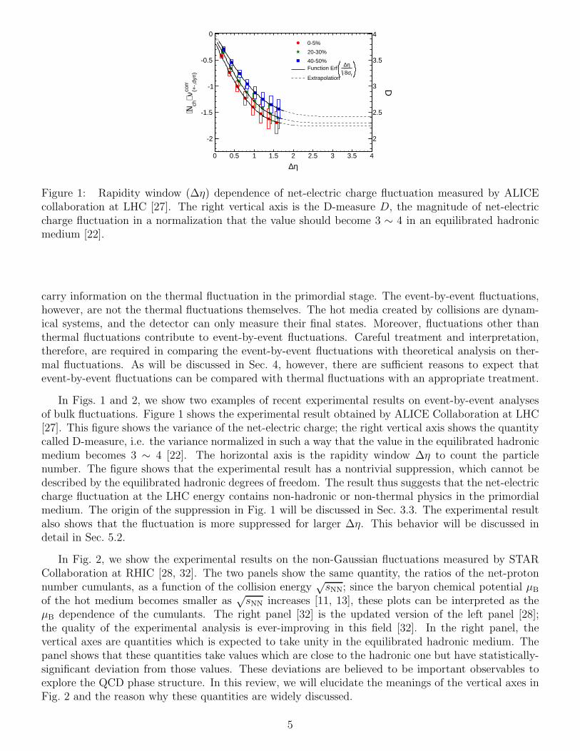


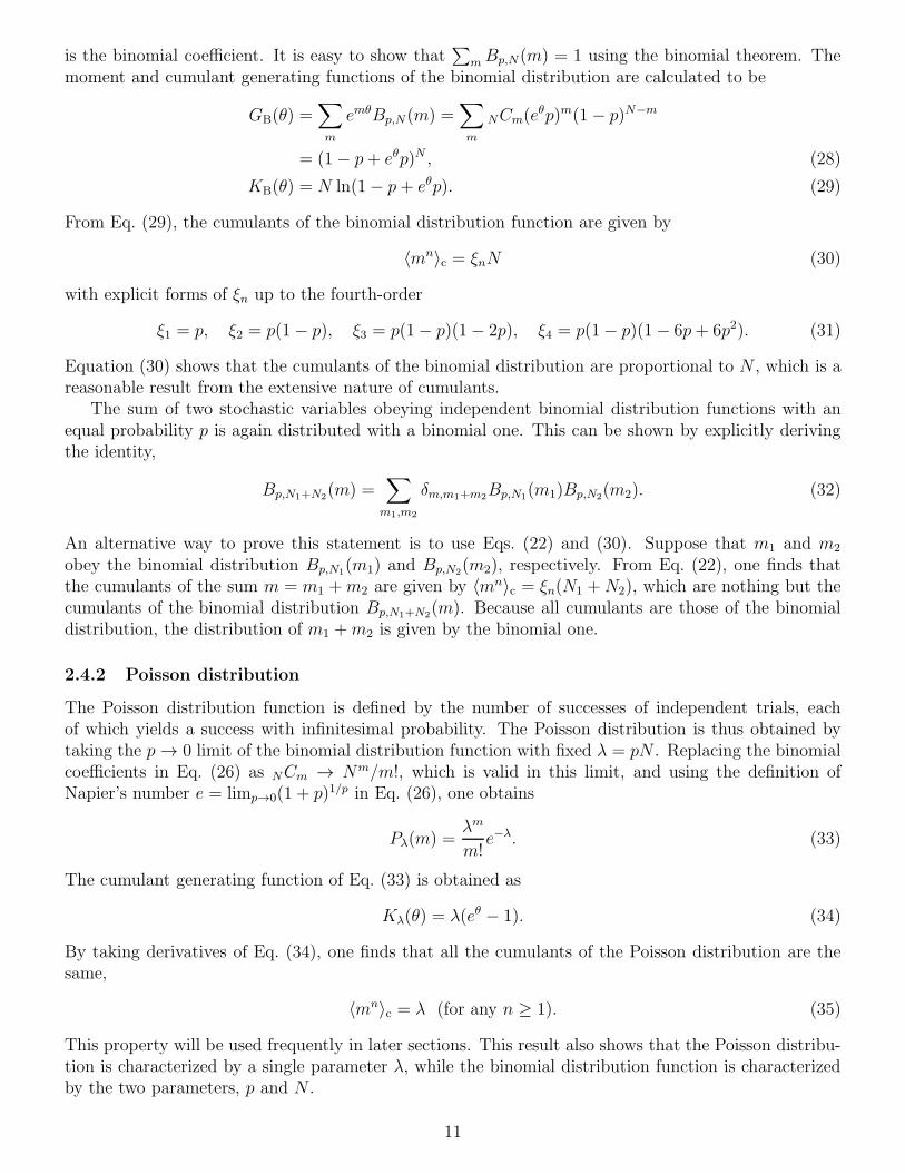
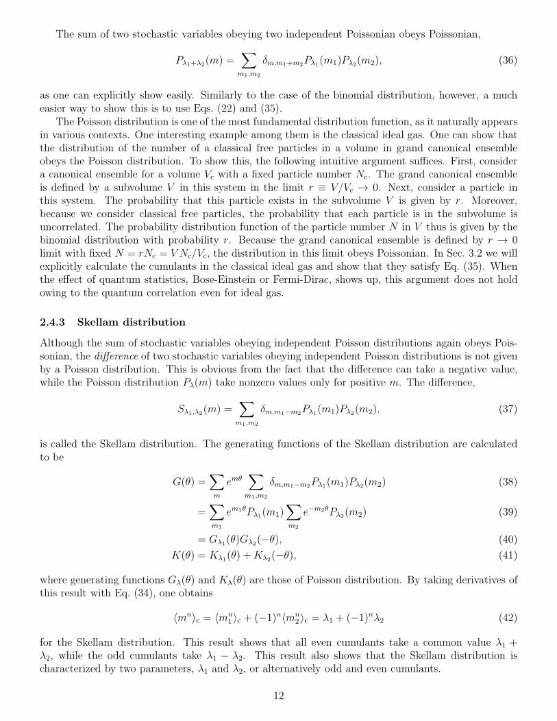

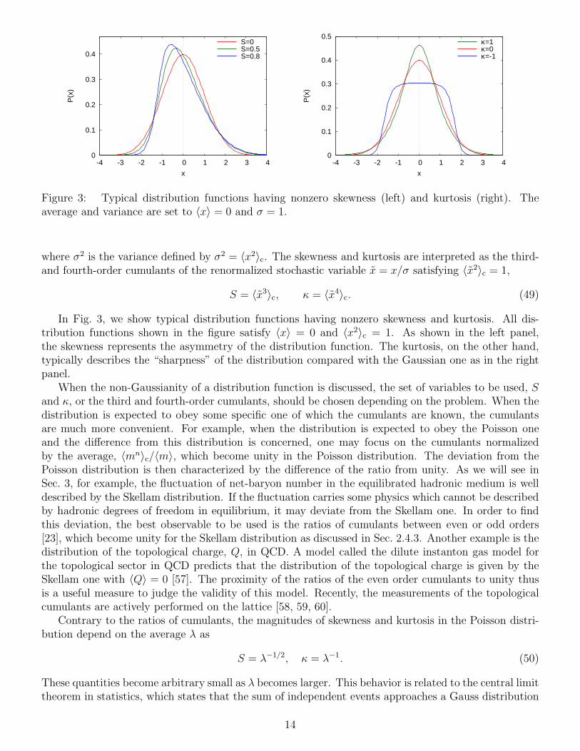


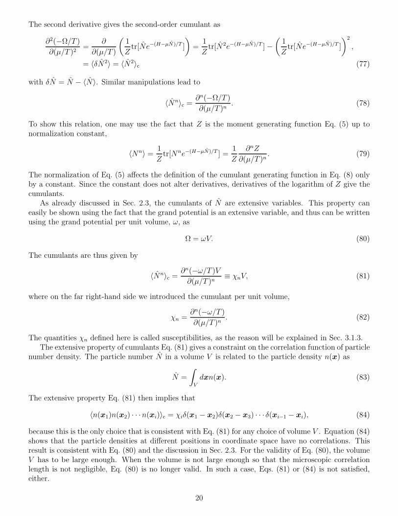


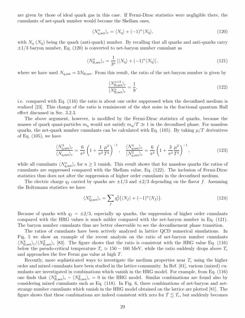


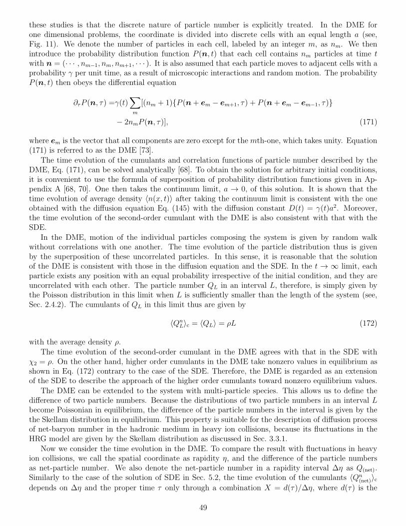


![OpenQuantumSystems. AnIntroduction Angel Rivas … › pdf › 1104.5242.pdf · 2013-07-29 · arXiv:1104.5242v2 [quant-ph] 9 Feb 2012 OpenQuantumSystems. AnIntroduction Angel Rivas´](https://static.documents.pub/doc/80x56/5f19b71fe3f0ff5e0b15e7ae/openquantumsystems-anintroduction-angel-rivas-a-pdf-a-11045242pdf-2013-07-29.jpg)


