50
1 © 2015 ANSYS, Inc. February 13, 2015 ANSYS Confidential 16.0 Release Lecture 7: Turbulence Modeling Introduction to ANSYS Fluent
| Date post: | 16-Jul-2016 |
| Category: |
Documents |
| Upload: | daniel-castro |
| View: | 316 times |
| Download: | 76 times |
1 © 2015 ANSYS, Inc. February 13, 2015 ANSYS Confidential
16.0 Release
Lecture 7:
Turbulence Modeling
Introduction to ANSYS Fluent
2 © 2015 ANSYS, Inc. February 13, 2015 ANSYS Confidential
Lecture Theme:
The majority of engineering flows are turbulent. Simulating turbulent flows in Fluent requires activating a turbulence model, selecting a near-wall modeling approach and providing inlet boundary conditions for the turbulence model.
Learning Aims:
You will learn: • How to use the Reynolds number to determine whether the flow is turbulent • How to select the turbulence model • How to choose which approach to use for modeling flow near walls • How to specify turbulence boundary conditions at inlets
Learning Objectives:
You will be able to determine whether a flow is turbulent and be able to set up and solve turbulent flow problems
Introduction
Introduction Reynolds Number Models Near-Wall Treatments Inlet BCs Summary
3 © 2015 ANSYS, Inc. February 13, 2015 ANSYS Confidential
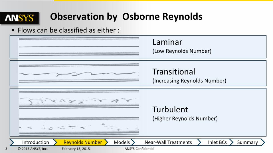
• Flows can be classified as either :
Laminar (Low Reynolds Number)
Transitional (Increasing Reynolds Number)
Turbulent (Higher Reynolds Number)
Observation by Osborne Reynolds
Introduction Reynolds Number Models Near-Wall Treatments Inlet BCs Summary

4 © 2015 ANSYS, Inc. February 13, 2015 ANSYS Confidential
Reynolds Number
• The Reynolds number is the criterion used to determine whether the flow is laminar or turbulent
• The Reynolds number is based on the length scale of the flow:
• Transition to turbulence varies depending on the type of flow:
• External flow
• along a surface : ReX > 500 000
• around on obstacle : ReL > 20 000
• Internal flow : ReD > 2 300
. .ReL
U L
etc. ,d d, x,L hyd
Introduction Reynolds Number Models Near-Wall Treatments Inlet BCs Summary
5 © 2015 ANSYS, Inc. February 13, 2015 ANSYS Confidential
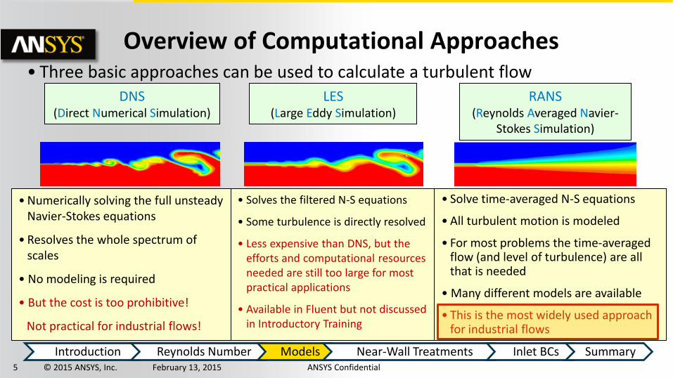
Overview of Computational Approaches • Three basic approaches can be used to calculate a turbulent flow
DNS (Direct Numerical Simulation)
• Numerically solving the full unsteady Navier-Stokes equations
• Resolves the whole spectrum of scales
• No modeling is required
• But the cost is too prohibitive!
Not practical for industrial flows!
• Solves the filtered N-S equations
• Some turbulence is directly resolved
• Less expensive than DNS, but the efforts and computational resources needed are still too large for most practical applications
• Available in Fluent but not discussed in Introductory Training
• Solve time-averaged N-S equations
• All turbulent motion is modeled
• For most problems the time-averaged flow (and level of turbulence) are all that is needed
• Many different models are available
• This is the most widely used approach for industrial flows
LES (Large Eddy Simulation)
RANS (Reynolds Averaged Navier-
Stokes Simulation)
Introduction Reynolds Number Models Near-Wall Treatments Inlet BCs Summary
6 © 2015 ANSYS, Inc. February 13, 2015 ANSYS Confidential
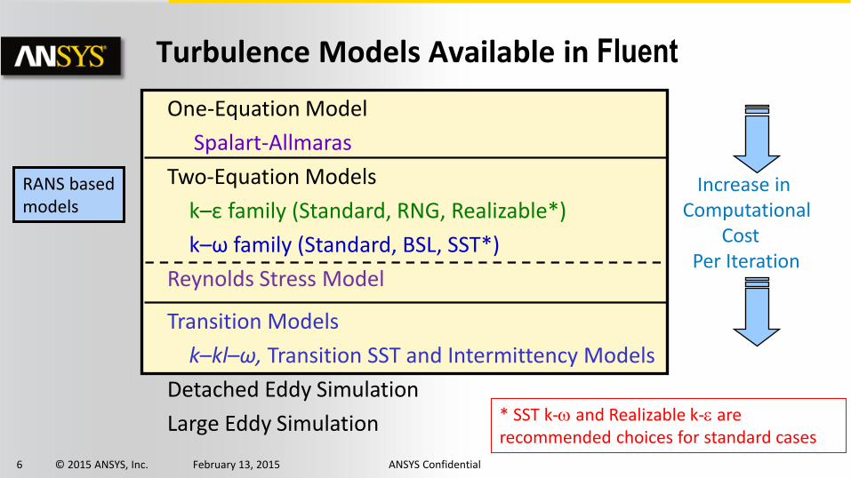
Turbulence Models Available in Fluent
RANS based models
One-Equation Model
Spalart-Allmaras
Two-Equation Models
k–ε family (Standard, RNG, Realizable*)
k–ω family (Standard, BSL, SST*)
Reynolds Stress Model
Transition Models
k–kl–ω, Transition SST and Intermittency Models
Detached Eddy Simulation
Large Eddy Simulation
Increase in Computational Cost Per Iteration
* SST k-w and Realizable k-e are recommended choices for standard cases

7 © 2015 ANSYS, Inc. February 13, 2015 ANSYS Confidential
RANS Turbulence Model Usage
Model Behavior and Usage
Spalart-Allmaras Economical for large meshes. Good for mildly complex (quasi-2D) external/internal flows and boundary layer flows under pressure
gradient (e.g. airfoils, wings, airplane fuselages, missiles, ship hulls). Performs poorly for 3D flows, free shear flows, flows with strong
separation.
Standard k–ε Robust. Widely used despite the known limitations of the model. Performs poorly for complex flows involving severe pressure gradient,
separation, strong streamline curvature. Suitable for initial iterations, initial screening of alternative designs, and parametric studies.
Realizable k–ε* Suitable for complex shear flows involving rapid strain, moderate swirl, vortices, and locally transitional flows (e.g. boundary layer
separation, massive separation, and vortex shedding behind bluff bodies, stall in wide-angle diffusers, room ventilation).
RNG k–ε Offers largely the same benefits and has similar applications as Realizable. Possibly harder to converge than Realizable.
Standard k–ω Superior performance for wall-bounded boundary layer, free shear, and low Reynolds number flows compared to models from the k-e
family. Suitable for complex boundary layer flows under adverse pressure gradient and separation (external aerodynamics and
turbomachinery). Separation can be predicted to be excessive and early.
SST k–ω* Offers similar benefits as standard k–ω. Not overly sensitive to inlet boundary conditions like the standard k–ω. Provides more accurate
prediction of flow separation than other RANS models.
BSL k–ω Similar to SST k-w. Good for some complex flows if SST model is overpredicting flow separation
RSM Physically the most sound RANS model. Avoids isotropic eddy viscosity assumption. More CPU time and memory required. Tougher to
converge due to close coupling of equations. Suitable for complex 3D flows with strong streamline curvature, strong swirl/rotation (e.g.
curved duct, rotating flow passages, swirl combustors with very large inlet swirl, cyclones).
* Realizable k-e or SST k-w are the recommended choice for standard cases
8 © 2015 ANSYS, Inc. February 13, 2015 ANSYS Confidential
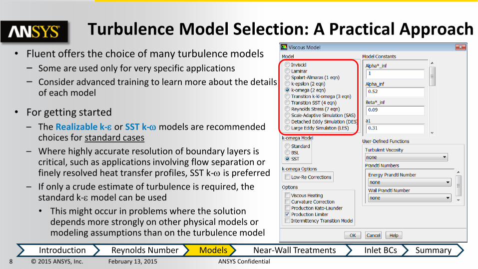
Turbulence Model Selection: A Practical Approach • Fluent offers the choice of many turbulence models
‒ Some are used only for very specific applications
‒ Consider advanced training to learn more about the details of each model
• For getting started
– The Realizable k-e or SST k-w models are recommended choices for standard cases
– Where highly accurate resolution of boundary layers is critical, such as applications involving flow separation or finely resolved heat transfer profiles, SST k-w is preferred
– If only a crude estimate of turbulence is required, the standard k-e model can be used
• This might occur in problems where the solution depends more strongly on other physical models or modeling assumptions than on the turbulence model
Introduction Reynolds Number Models Near-Wall Treatments Inlet BCs Summary

9 © 2015 ANSYS, Inc. February 13, 2015 ANSYS Confidential
• A turbulent boundary layer consists of distinct regions
• For CFD, the most important are the viscous sublayer, immediately adjacent to the wall and the log-layer, slightly further away from the wall
• Different turbulence models require different inputs depending on whether the simulation needs to resolve the viscous sublayer with the mesh ‒ This is an important consideration in a
turbulent flow simulation and will be described in the next few slides
Turbulent Boundary Layers
viscous
Introduction Reynolds Number Models Near-Wall Treatments Inlet BCs Summary
10 © 2015 ANSYS, Inc. February 13, 2015 ANSYS Confidential
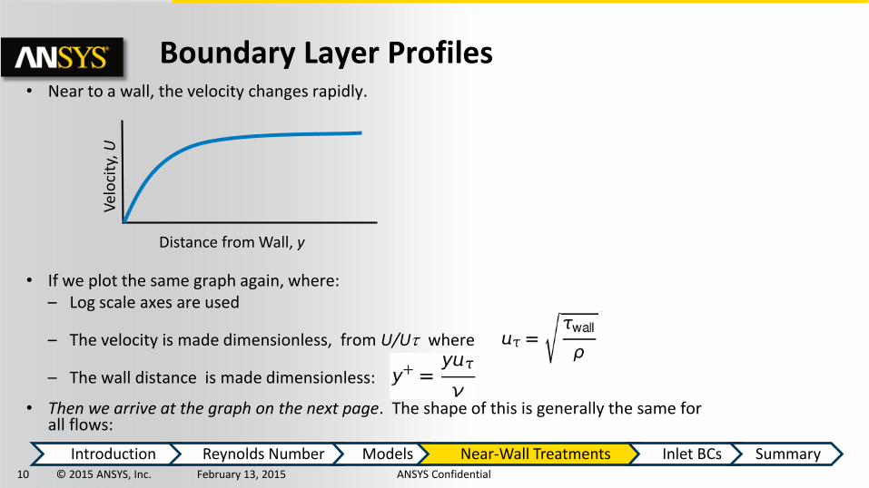
• Near to a wall, the velocity changes rapidly.
• If we plot the same graph again, where: – Log scale axes are used
– The velocity is made dimensionless, from U/Ut where
– The wall distance is made dimensionless:
• Then we arrive at the graph on the next page. The shape of this is generally the same for all flows:
Boundary Layer Profiles
Vel
oci
ty, U
Distance from Wall, y
Introduction Reynolds Number Models Near-Wall Treatments Inlet BCs Summary

11 © 2015 ANSYS, Inc. February 13, 2015 ANSYS Confidential
• By scaling the variables near the wall the velocity profile data takes on a predictable form (transitioning from linear in the viscous sublayer to logarithmic behavior in the log-layer)
Linear Logarithmic
Using the non-dimensional velocity and non-dimensional distance from the wall results in a predictable boundary layer profile for a wide range of flows
Dimensionless Boundary Layer Profiles
As the system Reynolds number increases, the logarithmic region extends to higher values of y+
Introduction Reynolds Number Models Near-Wall Treatments Inlet BCs Summary
12 © 2015 ANSYS, Inc. February 13, 2015 ANSYS Confidential
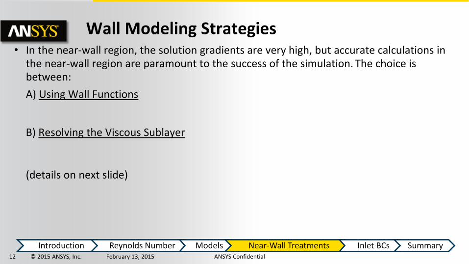
Wall Modeling Strategies • In the near-wall region, the solution gradients are very high, but accurate calculations in
the near-wall region are paramount to the success of the simulation. The choice is between:
A) Using Wall Functions
B) Resolving the Viscous Sublayer
(details on next slide)
Introduction Reynolds Number Models Near-Wall Treatments Inlet BCs Summary
13 © 2015 ANSYS, Inc. February 13, 2015 ANSYS Confidential
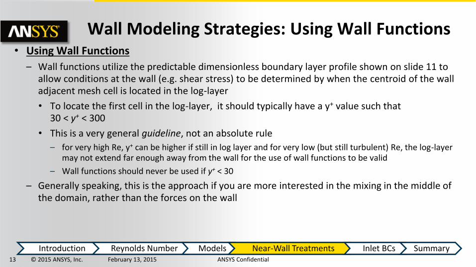
Wall Modeling Strategies: Using Wall Functions • Using Wall Functions
– Wall functions utilize the predictable dimensionless boundary layer profile shown on slide 11 to allow conditions at the wall (e.g. shear stress) to be determined by when the centroid of the wall adjacent mesh cell is located in the log-layer
• To locate the first cell in the log-layer, it should typically have a y+ value such that 30 < y+ < 300
• This is a very general guideline, not an absolute rule
– for very high Re, y+ can be higher if still in log layer and for very low (but still turbulent) Re, the log-layer may not extend far enough away from the wall for the use of wall functions to be valid
– Wall functions should never be used if y+ < 30
– Generally speaking, this is the approach if you are more interested in the mixing in the middle of the domain, rather than the forces on the wall
Introduction Reynolds Number Models Near-Wall Treatments Inlet BCs Summary
14 © 2015 ANSYS, Inc. February 13, 2015 ANSYS Confidential
Wall Modeling Strategies: Resolving the Viscous Sublayer
• Resolving the Viscous Sublayer
• First grid cell needs to be at about y+ ≈ 1 and a prism layer mesh with growth rate no higher than ≈ 1.2 should be used
– These are not magic numbers – this guideline ensures the mesh will be able to adequately resolve gradients in the sublayer
• This will add significantly to the mesh count (see next slide)
• Generally speaking, if the forces or heat transfer on the wall are key to your simulation (aerodynamic drag, turbomachinery blade performance, heat transfer) this is the approach you will take and the recommended turbulence model for most cases is SST k-w
Introduction Reynolds Number Models Near-Wall Treatments Inlet BCs Summary
15 © 2015 ANSYS, Inc. February 13, 2015 ANSYS Confidential
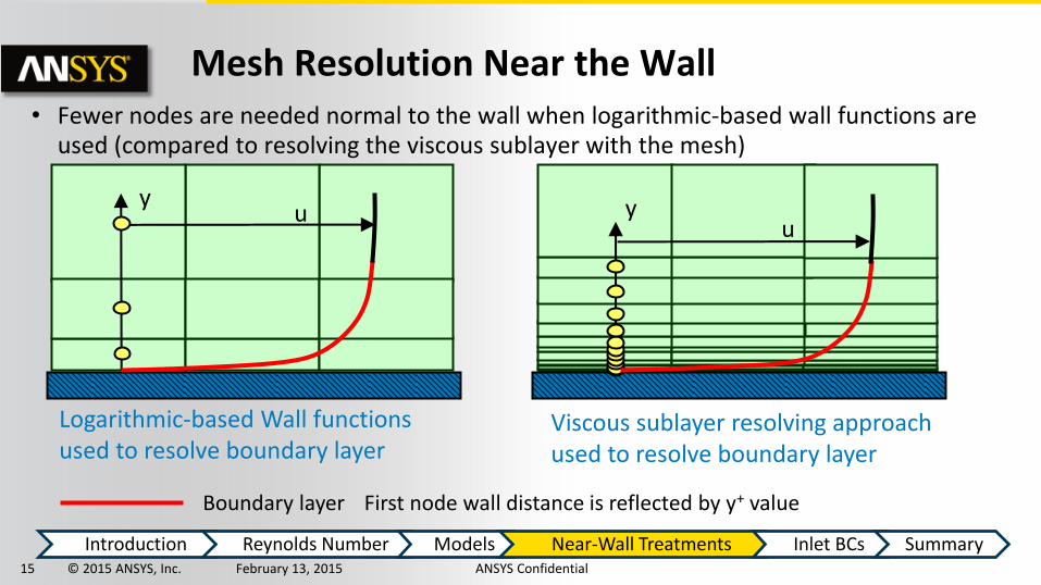
• Fewer nodes are needed normal to the wall when logarithmic-based wall functions are used (compared to resolving the viscous sublayer with the mesh)
u y
u y
Boundary layer
Logarithmic-based Wall functions used to resolve boundary layer
Viscous sublayer resolving approach used to resolve boundary layer
First node wall distance is reflected by y+ value
Mesh Resolution Near the Wall
Introduction Reynolds Number Models Near-Wall Treatments Inlet BCs Summary

16 © 2015 ANSYS, Inc. February 13, 2015 ANSYS Confidential
Example in Predicting Near-wall Cell Size • During the pre-processing stage, you will need to know a suitable size for the first layer of grid
cells (inflation layer) so that Y+ is in the desired range
• The actual flow-field will not be known until you have computed the solution (and indeed it is sometimes unavoidable to have to go back and remesh your model on account of the computed Y+ values)
• To reduce the risk of needing to remesh, you may want to try and predict the cell size by performing a hand calculation at the start, for example:
• For a flat plate, Reynolds number ( ) gives Rel = 1.4x10⁶
Recall from earlier slide, flow over a surface is turbulent when ReL > 5x10⁵
Flat plate, 1m long
Air at 20 m/s = 1.225 kg/m3
= 1.8x10⁻⁵ kg/ms
y
The question is what height (y) should the first row of grid cells be. We will use SWF, and are aiming for Y+ 50
VLl Re
Introduction Reynolds Number Models Near-Wall Treatments Inlet BCs Summary

17 © 2015 ANSYS, Inc. February 13, 2015 ANSYS Confidential
• Re is known, so use the definitions to calculate the first cell height
• We know we are aiming for y+ of 50, hence:
our first cell height y should be approximately 1 mm.
Calculating Wall Distance for a Given y+
• Begin with the definition of y+ and rearrange:
• The target y+ value and fluid properties are known, so we need Ut, which is defined as:
• The wall shear stress ,tw ,can be found from the skin friction coefficient, Cf:
• A literature search suggests a formula for the skin friction on a plate1 thus:
1 An equivalent formula for internal flows, with Reynolds number based on the pipe diameter is Cf = 0.079 Red-0.25
2.0Re058.0 lfC
221
UC fw t
tt
wU
tU
yy
t yUy
mU
yy 4-9x10
t
m/s 0.82
tt
wU
22
21 smkg/ 0.83 UC fw t
.0034 Re058.0 2.0
lfC
Introduction Reynolds Number Models Near-Wall Treatments Inlet BCs Summary

18 © 2015 ANSYS, Inc. February 13, 2015 ANSYS Confidential
• In some situations, such as boundary layer separation, logarithmic-based wall functions do not correctly predict the boundary layer profile
• In these cases logarithmic-based wall functions should not be used
• Instead, directly resolving the viscous sublayer with the mesh can provide accurate results
Wall functions applicable Wall functions not applicable
Limitations of Wall Functions
Non-equilibrium wall functions have been developed in Fluent to address this situation but they are very empirical. Resolving the viscous sublayer with the mesh is recommended if affordable
Introduction Reynolds Number Models Near-Wall Treatments Inlet BCs Summary

19 © 2015 ANSYS, Inc. February 13, 2015 ANSYS Confidential
• If the viscous sublayer is being resolved – Use k-w models or k-e models with Enhanced Wall Treatment
(EWT)
– No separate input is needed for k-w models
• If wall functions are used – Use k-e models with wall functions
• EWT can also be used because it is a y+ insensitive method and will act like a wall function if the first grid point is in the log-layer
– For k-w models
• The k-w models utilize a y+ insensitive wall treatment and will act like a wall function if the first grid point is in the log layer
• However, the advantages of these models may be lost when a coarse near-wall mesh is used
Turbulence Settings for Near Wall Modeling
Introduction Reynolds Number Models Near-Wall Treatments Inlet BCs Summary

20 © 2015 ANSYS, Inc. February 13, 2015 ANSYS Confidential
Inlet Boundary Conditions • When turbulent flow enters a domain at inlets or outlets (backflow), boundary conditions
must be given for the turbulence model variables
• Four methods for specifying turbulence boundary conditions:
1) Turbulent intensity and viscosity ratio (default)
Default values of turbulent intensity = 5% and turbulent viscosity ratio = 10 are reasonable for cases where you have no information about turbulence at an inlet
2) Turbulent intensity and length scale • Length scale is related to size of large eddies that contain most of energy
– For boundary layer flows: l 0.4δ99
– For flows downstream of grid: l opening size
3) Turbulent intensity and hydraulic diameter (primarily for internal flows)
4) Explicitly input k, ε, ω, or Reynolds stress components (this is the only method that allows for profile definition)
Introduction Reynolds Number Models Near-Wall Treatments Inlet BCs Summary
21 © 2015 ANSYS, Inc. February 13, 2015 ANSYS Confidential
Guidelines for Inlet Turbulence Conditions • If you have absolutely no idea of the turbulence levels in your simulation, you could use
following values of turbulence intensities and viscosity ratios:
– Normal turbulent intensities range from 1% to 5%
– The default turbulent intensity value 5% is sufficient for nominal turbulence through a circular inlet, and is a good estimate in the absence of experimental data
– For external flows, turbulent viscosity ratio of 1-10 is typically a good value
– For internal flows, turbulent viscosity ratio of 10-100 it typically a good value
• For fully developed pipe flow at Re = 50,000, the turbulent viscosity ratio is around 100
Introduction Reynolds Number Models Near-Wall Treatments Inlet BCs Summary

22 © 2015 ANSYS, Inc. February 13, 2015 ANSYS Confidential
Summary – Turbulence Modeling Guidelines
• To perform a turbulent flow calculation in Fluent
‒ Calculate the Reynolds number and determine whether flow is turbulent.
‒ Decide on a near-wall modeling strategy
• The choices are A) Resolve the viscous sublayer or B) Use wall functions
• Create the mesh with y+ suitable for the selected approach
‒ Choose turbulence model and near wall treatment (if necessary) in the Viscous Models panel
• Realizable k-e or SST k-w are recommended choices for standard cases
• SST k-w is preferred for cases where the viscous sublayer needs to be resolved (flow separation, detailed heat transfer)
‒ Set reasonable boundary conditions for the turbulence model variables
Introduction Reynolds Number Models Near-Wall Treatments Inlet BCs Summary

23 © 2015 ANSYS, Inc. February 13, 2015 ANSYS Confidential
Appendix
24 © 2015 ANSYS, Inc. February 13, 2015 ANSYS Confidential
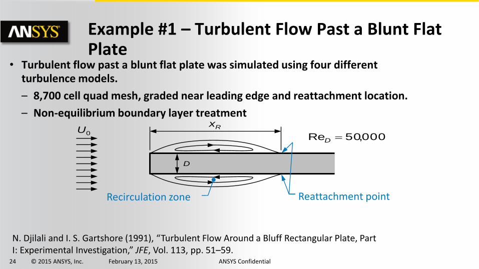
Example #1 – Turbulent Flow Past a Blunt Flat Plate
• Turbulent flow past a blunt flat plate was simulated using four different turbulence models.
– 8,700 cell quad mesh, graded near leading edge and reattachment location.
– Non-equilibrium boundary layer treatment
N. Djilali and I. S. Gartshore (1991), “Turbulent Flow Around a Bluff Rectangular Plate, Part I: Experimental Investigation,” JFE, Vol. 113, pp. 51–59.
D
000,50Re D
Rx
Recirculation zone Reattachment point
0U
25 © 2015 ANSYS, Inc. February 13, 2015 ANSYS Confidential
RNG k–ε Standard k–ε
Reynolds Stress Realizable k–ε
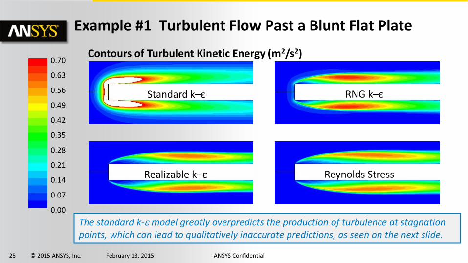
Contours of Turbulent Kinetic Energy (m2/s2)
0.00
0.07
0.14
0.21
0.28
0.35
0.42
0.49
0.56
0.63
0.70
Example #1 Turbulent Flow Past a Blunt Flat Plate
The standard k-e model greatly overpredicts the production of turbulence at stagnation points, which can lead to qualitatively inaccurate predictions, as seen on the next slide.

26 © 2015 ANSYS, Inc. February 13, 2015 ANSYS Confidential
Experimentally observed reattachment point is at x / D = 4.7
Predicted separation bubble:
Standard k–ε (SKE) Skin Friction
Coefficient Cf × 1000
SKE severely underpredicts the size of the separation bubble, while RKE predicts the size exactly.
Realizable k–ε (RKE)
Distance Along Plate, x / D
Example #1 Turbulent Flow Past a Blunt Flat Plate
27 © 2015 ANSYS, Inc. February 13, 2015 ANSYS Confidential
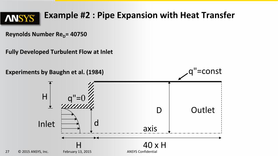
Reynolds Number ReD= 40750
Fully Developed Turbulent Flow at Inlet
Experiments by Baughn et al. (1984) q"=const
Outlet
axis
H
H 40 x H
Inlet
q"=0
d
D
Example #2 : Pipe Expansion with Heat Transfer

28 © 2015 ANSYS, Inc. February 13, 2015 ANSYS Confidential
• Plot shows dimensionless distance versus Nusselt Number
• Best agreement is with SST and k-omega models which do a better job of capturing flow recirculation zones accurately
Example #2 : Pipe Expansion with Heat Transfer

29 © 2015 ANSYS, Inc. February 13, 2015 ANSYS Confidential
• 40,000-cell hexahedral mesh
• High-order upwind scheme was used.
• Computed using SKE, RNG, RKE and RSM (second moment closure) models with the standard wall functions
• Represents highly swirling flows (Wmax = 1.8 Uin)
0.2 m
Uin = 20 m/s
0.97 m
0.1 m
0.12 m
Example #3 Turbulent Flow in a Cyclone
30 © 2015 ANSYS, Inc. February 13, 2015 ANSYS Confidential
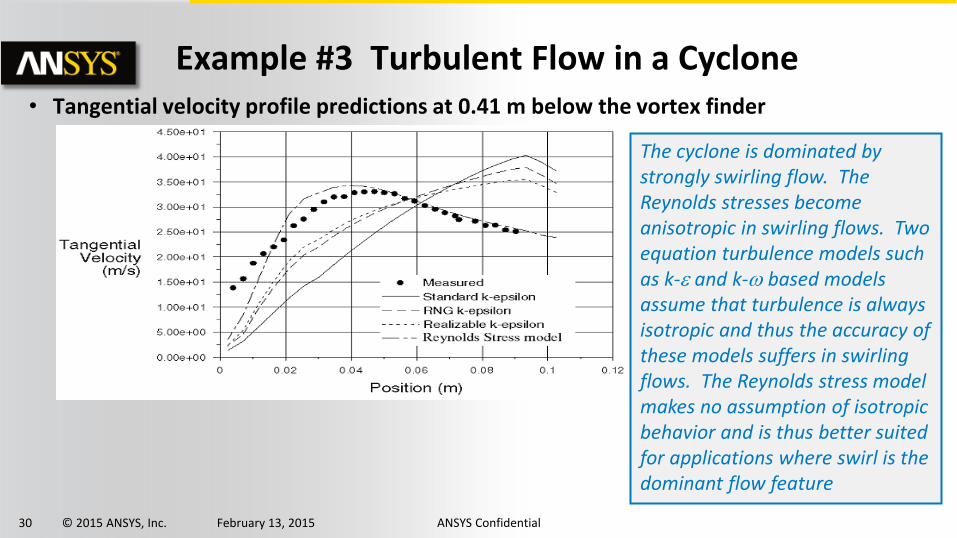
• Tangential velocity profile predictions at 0.41 m below the vortex finder
Example #3 Turbulent Flow in a Cyclone
The cyclone is dominated by strongly swirling flow. The Reynolds stresses become anisotropic in swirling flows. Two equation turbulence models such as k-e and k-w based models assume that turbulence is always isotropic and thus the accuracy of these models suffers in swirling flows. The Reynolds stress model makes no assumption of isotropic behavior and is thus better suited for applications where swirl is the dominant flow feature

31 © 2015 ANSYS, Inc. February 13, 2015 ANSYS Confidential
Shear Stress Transport (SST) Model
• It accounts more accurately for the transport of the turbulent shear stress, which improves predictions of the onset and the amount of flow separation compared to k-e models
SST result and experiment
Standard k-e fails to predict separation
Experiment Gersten et al.
Example 4: Diffuser
32 © 2015 ANSYS, Inc. February 13, 2015 ANSYS Confidential
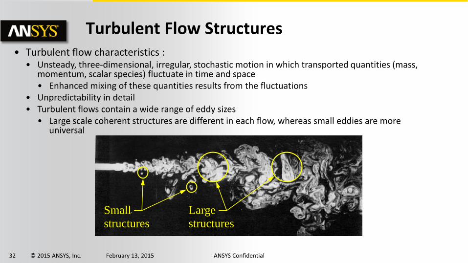
• Turbulent flow characteristics : • Unsteady, three-dimensional, irregular, stochastic motion in which transported quantities (mass,
momentum, scalar species) fluctuate in time and space • Enhanced mixing of these quantities results from the fluctuations
• Unpredictability in detail • Turbulent flows contain a wide range of eddy sizes
• Large scale coherent structures are different in each flow, whereas small eddies are more universal
Turbulent Flow Structures
Small
structures
Large
structures

33 © 2015 ANSYS, Inc. February 13, 2015 ANSYS Confidential
Energy Cascade
• Energy is transferred from larger eddies to smaller eddies
• Larger eddies contain most of the energy
• In the smallest eddies, turbulent energy is converted to internal energy by viscous dissipation
Energy Cascade Richardson
(1922), Kolmogorov (1941)
34 © 2015 ANSYS, Inc. February 13, 2015 ANSYS Confidential
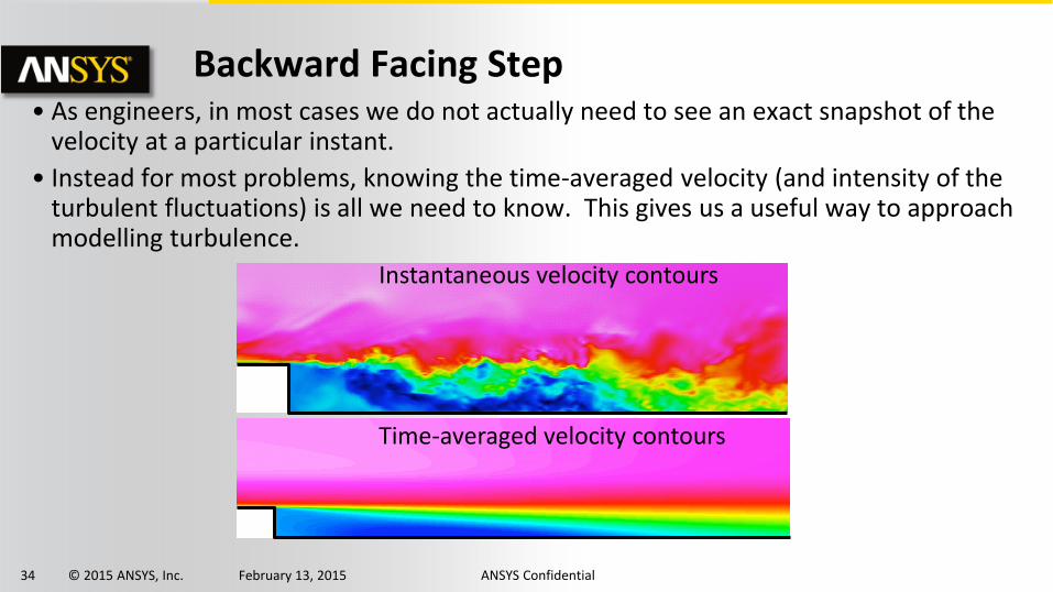
Backward Facing Step
Instantaneous velocity contours
Time-averaged velocity contours
• As engineers, in most cases we do not actually need to see an exact snapshot of the velocity at a particular instant.
• Instead for most problems, knowing the time-averaged velocity (and intensity of the turbulent fluctuations) is all we need to know. This gives us a useful way to approach modelling turbulence.

35 © 2015 ANSYS, Inc. February 13, 2015 ANSYS Confidential
• If we recorded the velocity at a particular point in the real (turbulent) fluid flow, the instantaneous velocity (U) would look like this:
Time-average of velocity V
elo
city
U Instantaneous velocity
U
uFluctuating velocity
• At any point in time:
• The time average of the fluctuating velocity must be zero:
• BUT, the RMS of is not necessarily zero: • The turbulent energy, k, is given by the fluctuating velocity components as:
uUU
0u
u 02 u 222
2
1wvuk
Time
Mean and Instantaneous Velocities
36 © 2015 ANSYS, Inc. February 13, 2015 ANSYS Confidential
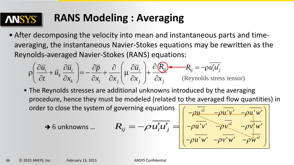
RANS Modeling : Averaging
• After decomposing the velocity into mean and instantaneous parts and time-averaging, the instantaneous Navier-Stokes equations may be rewritten as the Reynolds-averaged Navier-Stokes (RANS) equations:
• The Reynolds stresses are additional unknowns introduced by the averaging procedure, hence they must be modeled (related to the averaged flow quantities) in order to close the system of governing equations
jiij uuR 6 unknowns …
jiij uuR
j
ij
j
i
jik
ik
i
x
R
x
u
xx
p
x
uu
t
u
(Reynolds stress tensor)
2
2
2
' ' ' ' '
' ' ' ' '
' ' ' ' '
xx xy xz
yx yy yz
zx zy zz
u u v u w
u v v v w
u w v w w
t t t
t t t
t t t
τ
37 © 2015 ANSYS, Inc. February 13, 2015 ANSYS Confidential
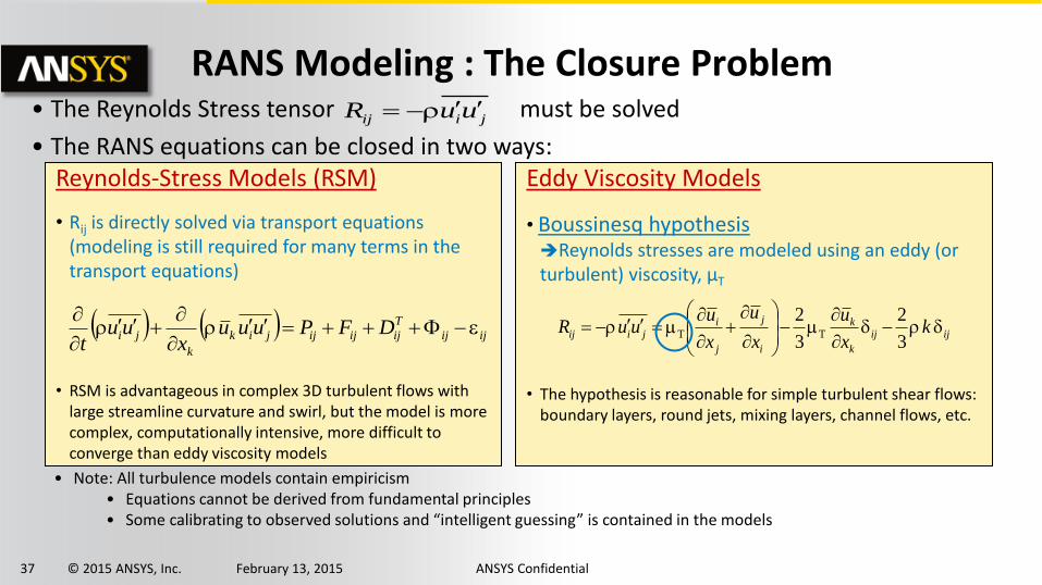
• The Reynolds Stress tensor must be solved
• The RANS equations can be closed in two ways:
Eddy Viscosity Models
• Boussinesq hypothesis Reynolds stresses are modeled using an eddy (or turbulent) viscosity, μT
• The hypothesis is reasonable for simple turbulent shear flows:
boundary layers, round jets, mixing layers, channel flows, etc.
RANS Modeling : The Closure Problem
Reynolds-Stress Models (RSM)
• Rij is directly solved via transport equations (modeling is still required for many terms in the
transport equations)
• RSM is advantageous in complex 3D turbulent flows with
large streamline curvature and swirl, but the model is more complex, computationally intensive, more difficult to converge than eddy viscosity models
jiij uuR
ijij
T
ijijijjik
k
ji DFPuuux
uut
e
ijij
k
k
i
j
j
ijiij k
x
u
x
u
x
uuuR
3
2
3
2TT
• Note: All turbulence models contain empiricism • Equations cannot be derived from fundamental principles • Some calibrating to observed solutions and “intelligent guessing” is contained in the models

38 © 2015 ANSYS, Inc. February 13, 2015 ANSYS Confidential
Two-Equation Models • Two transport equations are solved, giving two independent scales for
calculating t
– Virtually all use the transport equation for the turbulent kinetic energy, k – Several transport variables have been proposed, based on dimensional arguments, and used
for second equation. The eddy viscosity t is then formulated from the two transport variables.
– Kolmogorov, w: t k / w, l k1/2 / w, k e / w
• w is specific dissipation rate • defined in terms of large eddy scales that define supply rate of k
– Chou, e: t k2 / e, l k3/2 / e – Rotta, l: t k1/2l, e k3/2 / l
ijijt
jkj
SSSskeSPPx
k
xDt
Dk2)(; 2t
e
production dissipation
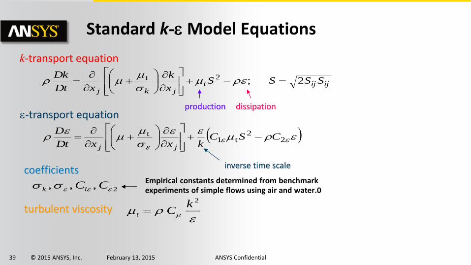
39 © 2015 ANSYS, Inc. February 13, 2015 ANSYS Confidential
Standard k-e Model Equations
Empirical constants determined from benchmark experiments of simple flows using air and water.0
ijijtjkj
SSSSx
k
xDt
Dk2;2t
e
eee
e ee
e2
2t1
t CSCkxxDt
D
jj
k-transport equation
e-transport equation production dissipation
2 , , , eee CCik
coefficients
turbulent viscosity e
2
k
Ct
inverse time scale
40 © 2015 ANSYS, Inc. February 13, 2015 ANSYS Confidential
RANS : EVM :Standard k–ε (SKE) Model • The Standard K-Epsilon model (SKE) is the most widely-used engineering turbulence
model for industrial applications
– Model parameters are calibrated by using data from a number of benchmark experiments such as pipe flow, flat plate, etc.
– Robust and reasonably accurate for a wide range of applications
– Contains submodels for compressibility, buoyancy, combustion, etc.
• Known limitations of the SKE model:
– Performs poorly for flows with larger pressure gradient, strong separation, high swirling component and large streamline curvature.
– Inaccurate prediction of the spreading rate of round jets.
– Production of k is excessive (unphysical) in regions with large strain rate (for example, near a stagnation point), resulting in very inaccurate model predictions.
41 © 2015 ANSYS, Inc. February 13, 2015 ANSYS Confidential
RANS : EVM: Realizable k-epsilon • Realizable k–ε (RKE) model (Shih):
– Dissipation rate (ε) equation is derived from the mean-square vorticity fluctuation, which is fundamentally different from the SKE.
– Several realizability conditions are enforced for Reynolds stresses.
– Benefits:
• Accurately predicts the spreading rate of both planar and round jets
• Also likely to provide superior performance for flows involving rotation, boundary layers under strong adverse pressure gradients, separation, and recirculation
OFTEN PREFERRED TO STANDARD K-EPSILON.

42 © 2015 ANSYS, Inc. February 13, 2015 ANSYS Confidential
RANS : EVM : Spalart-Allmaras (S-A) Model
• Spalart-Allmaras is a low-cost RANS model solving a single transport equation for a modified eddy viscosity
• Designed specifically for aerospace applications involving wall-bounded flows
– Has been shown to give good results for boundary layers subjected to adverse pressure gradients.
– Used mainly for aerospace and turbomachinery applications
• Limitations:
– The model was designed for wall bounded flows and flows with mild separation and recirculation.
– No claim is made regarding its applicability to all types of complex engineering flows.
43 © 2015 ANSYS, Inc. February 13, 2015 ANSYS Confidential
• In k-w models, the transport equation for the turbulent dissipation rate, e, is replaced with an equation for the specific dissipation rate, w
– The turbulent kinetic energy transport equation is still solved
• k-w models have gained popularity in recent years mainly because:
– Much better performance than k-e models for boundary layer flows
• For separation, transition, low Re effects, and impingement, k-w models are more accurate than k-e models
– Accurate and robust for a wide range of boundary layer flows with pressure gradient
• Two variations of the k-w model are available in Fluent – Standard k-w model (Wilcox, 1998)
– SST k-w model (Menter)
k-omega Models

44 © 2015 ANSYS, Inc. February 13, 2015 ANSYS Confidential
• k-w models are RANS two-equations based models
• One of the advantages of the k-w formulation is the near wall treatment for low-Reynolds number computations – designed to predict correct behavior when integrated to the wall
• the k-w models switches between a viscous sublayer formulation (i.e. direct resolution of the boundary layer) at low y+ values and a wall function approach at higher y+ values
– while k-e model variations require Enhanced Wall Treatment to capture correct viscous sublayer behavior
k-omega Model
j
t
jj
iij
jk
t
jj
iij
t
xxf
x
u
kDt
D
x
k
xkf
x
u
Dt
Dk
k
w
wt
w
w
wt
w
w
2
ω = specific dissipation rate
t
ew
1
k
ijij
k
k
i
j
j
ijiij k
x
u
x
u
x
uuuR
3
2
3
2TT

45 © 2015 ANSYS, Inc. February 13, 2015 ANSYS Confidential
• Shear Stress Transport (SST) Model • The SST model is a hybrid two-equation model that combines the advantages of both k-e and k-w
models – The k-w model performs much better than k-e models for boundary layer flows – Wilcox’ original k-w model is overly sensitive to the freestream value (BC) of w, while the k-e model is not
prone to such problems
• The k-e and k-w models are blended such that the SST model functions like the k-w close to the wall and the k-e
model in the freestream
SST is a good compromise between k-e and k-w models
SST Model
Wall
k-e
k-w

46 © 2015 ANSYS, Inc. February 13, 2015 ANSYS Confidential
RANS: Other Models in Fluent • RNG k-e model
– Model constants are derived from renormalization group (RNG) theory instead of empiricism
– Advantages over the standard k-e model are very similar to those of the RKE model
• Reynolds Stress model (RSM)
– Instead of using eddy viscosity to close the RANS equations, RSM solves transport equations for the individual Reynolds stresses
• 7 additional equations in 3D, compared to 2 additional equations with EVM.
– Much more computationally expensive than EVM and generally very difficult to converge
• As a result, RSM is used primarily in flows where eddy viscosity models are known to fail
• These are mainly flows where strong swirl is the predominant flow feature, for instance a cyclone

47 © 2015 ANSYS, Inc. February 13, 2015 ANSYS Confidential
Enhanced Wall Treatment (EWT) • Need for y+ insensitive wall
treatment
• EWT smoothly varies from low-Re to wall function with mesh resolution
• EWT available for k-e and RSM models
• Similar approach implemented for k-w equation based models, and for the Spalart-Allmaras model
The term "y+ insensitive wall treatment" does not mean the results will be identical no matter what the value of y+ is at the wall-adjacent cell. It means that as you refine the mesh, the solution will tend gradually towards grid independence. This is in contrast to wall functions, where the solution can be extremely sensitive to y+ values and grid independent solutions can be difficult to achieve.

48 © 2015 ANSYS, Inc. February 13, 2015 ANSYS Confidential
• The SST and k-w models were formulated to be near-wall resolving models where the viscous sublayer is resolved by the mesh
– To take full advantage of this formulation, y+ should be ≈ 1
– This is necessary for accurate prediction of flow separation
• These models can still be used with a coarser near-wall mesh and produce valid results, within the limitations of logarithmic wall functions
– The first grid point should still be in the logarithmic layer (y+ < 300 for most flows)
– Many advantages of these models may be lost when a coarse near-wall mesh is used
y+ for the SST and k-omega Models
49 © 2015 ANSYS, Inc. February 13, 2015 ANSYS Confidential
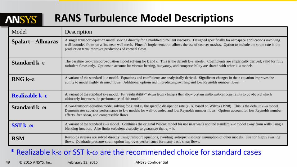
RANS Turbulence Model Descriptions
Model Description
Spalart – Allmaras A single transport equation model solving directly for a modified turbulent viscosity. Designed specifically for aerospace applications involving
wall-bounded flows on a fine near-wall mesh. Fluent’s implementation allows the use of coarser meshes. Option to include the strain rate in the
production term improves predictions of vortical flows.
Standard k–ε The baseline two-transport-equation model solving for k and ε. This is the default k–ε model. Coefficients are empirically derived; valid for fully
turbulent flows only. Options to account for viscous heating, buoyancy, and compressibility are shared with other k–ε models.
RNG k–ε A variant of the standard k–ε model. Equations and coefficients are analytically derived. Significant changes in the ε equation improves the
ability to model highly strained flows. Additional options aid in predicting swirling and low Reynolds number flows.
Realizable k–ε A variant of the standard k–ε model. Its “realizability” stems from changes that allow certain mathematical constraints to be obeyed which
ultimately improves the performance of this model.
Standard k–ω A two-transport-equation model solving for k and ω, the specific dissipation rate (ε / k) based on Wilcox (1998). This is the default k–ω model.
Demonstrates superior performance to k–ε models for wall-bounded and low Reynolds number flows. Options account for low Reynolds number
effects, free shear, and compressible flows.
SST k–ω A variant of the standard k–ω model. Combines the original Wilcox model for use near walls and the standard k–ε model away from walls using a
blending function. Also limits turbulent viscosity to guarantee that τT ~ k.
RSM Reynolds stresses are solved directly using transport equations, avoiding isotropic viscosity assumption of other models. Use for highly swirling
flows. Quadratic pressure-strain option improves performance for many basic shear flows.
* Realizable k-e or SST k-w are the recommended choice for standard cases
50 © 2015 ANSYS, Inc. February 13, 2015 ANSYS Confidential
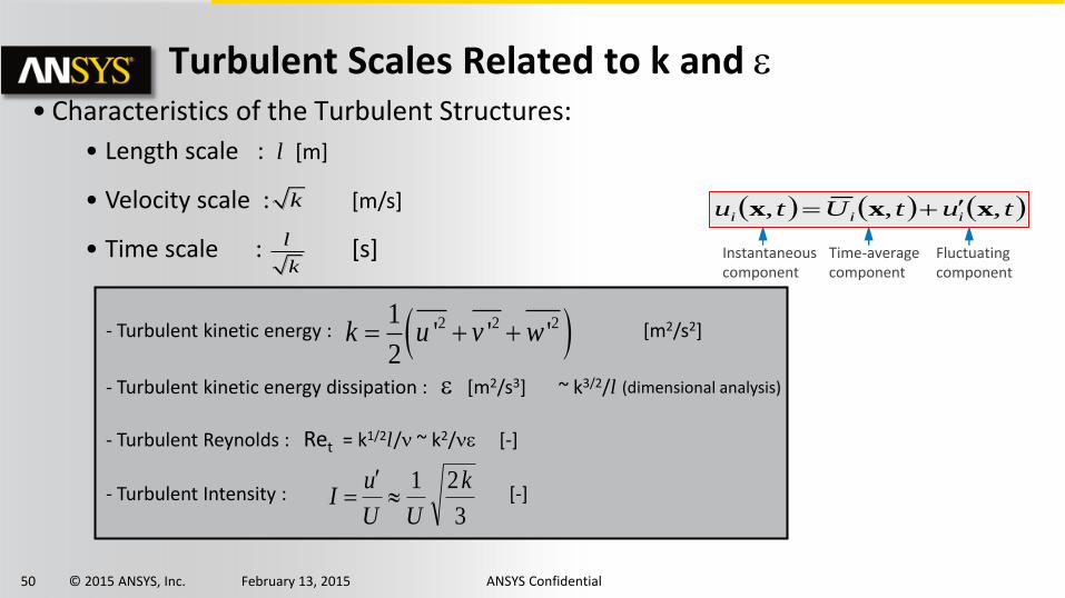
Turbulent Scales Related to k and e • Characteristics of the Turbulent Structures:
• Length scale : l [m]
• Velocity scale : [m/s]
• Time scale : [s]
k
l
k
- Turbulent kinetic energy : [m2/s2]
- Turbulent kinetic energy dissipation : e [m2/s3] ~ k3/2/l
- Turbulent Reynolds : Ret = k1/2l/n ~ k2/ne [-]
- Turbulent Intensity : [-]
2 2 21' ' '
2k u v w
%203
21
k
UU
uI
(dimensional analysis)
Fluctuating component
Time-average component
Instantaneous component
tutUtu iii ,,, xxx


