19
ME 360 Discharge through an Orifice F2 Date Performed: 2/17/15 Date Submitted: Part 2: 2/24/15 Name: Justin Carey
| Date post: | 21-Jul-2015 |
| Category: |
Documents |
| Upload: | justin-carey |
| View: | 40 times |
| Download: | 0 times |

ME 360
Discharge through an Orifice
F2
Date Performed: 2/17/15
Date Submitted: Part 2: 2/24/15
Name: Justin Carey

2 | P a g e
Introduction
There are many situations in the engineering field where it is necessary to know the flowrate
in a pipe. There are various flow-measuring devices that all determine the flow rate in a pipe but
the most common is the obstruction-type flowmeter. Obstruction flowmeters operate on the idea
that a decrease in flow area in a pipe causes an increase in velocity that in turn decreases
pressure. This correlation of pressure difference and velocity provides the means of measuring
flowrate. The different obstruction-type flowmeters consist of the orifice meter, the nozzle meter,
and the Venturi meter. In this lab we will be measuring the flow through an orifice meter. A
schematic of a standard orifice meter can be seen below in Figure 1.
Figure 1: Schematic of a standard orifice meter that is describe in the background.1
An orifice meter is defined to be a plate having a central hole that is placed across the
flow of a liquid, usually between flanges in a pipeline. The pressure difference generated by the
flow velocity through the hole enables the flow quantity to be measured (Dictionary.com). As
seen in Figure 1 the fluid flows in through the left side of the pipe at the pipe diameter D1 and is

3 | P a g e
restricted down to D2 as it flows through the restricting plates, this is known as the orifice. The
pressure difference is measured at P1 and P2. This pressure can be measured using any different
measurement devices such as piezometer tubes or pressure gages. The orifice meter also has
secondary flows that form within the pipe and contribute to error in the measurement of flow.
These secondary flows usually occur right after the orifice region of the meter and can be seen in
Figure 2 below.
Figure 2: Illustration of the secondary flows and vena contracta that occur in an orifice meter.2
Although in our lab experiment we will not have to deal with the secondary flows because
of the way our experimental apparatus is constructed. This will be explained later in detail in the
experimental method section of the report. Another phenomenon that occurs with an orifice meter
is the vena contracta. The vena contracta is the location of the smallest cross-sectional diameter of
the flow of liquid after the orifice of the meter. This is also shown in Figure 2 above. This
Secondary flows

4 | P a g e
phenomenon is the result of the inability of the fluid to turn the sharp 90 degree corner formed by
the orifice plates. Some common properties of the vena contracta are: constant pressure across the
cross-sectional area and all the streamlines of flow are parallel at this location (Fundamentals of
Fluid Mechanics). To calculate the theoretical flow rate through the meter you multiply the
velocity of the fluid by the area of the orifice. This value unfortunately will not match the actual
flow rate through the orifice of the meter. This is due to two main sources of error. The first is the
mechanical losses due to friction along the walls of the meter. The second is the reduction in area
of flow due to the vena contracta phenomenon discussed above. To account for these sources of
error a discharge coefficient is introduced into the calculation. According to
TheEngineeringToolBox.com a standard value for the discharge coefficient of an orifice meter is
0.6.
Objectives
To determine the discharge coefficient of the orifice meter.
Analytical Method
In order to complete the objective for this lab there are a series of equations that must be
derived from some basic physics equations such as the conservation of mass and energy. These
derivations will be worked out in this section of the report.
Unlike the general orifice meters described in the background that are horizontally
orientated, the meter we used in our lab was positioned vertically. A simple schematic of the
meter used can be seen below in Figure 3. For the following equations state 1 is located at M and
state 0 is located at N in the schematic.

5 | P a g e
Figure 3: A schematic of the orifice meter used taken from the lab handout
𝑃1
𝜌+
𝑈12
2+ 𝑔𝑧1 =
𝑃𝑜
𝜌+
𝑈𝑜2
2+ 𝑔𝑧2 + 𝑔ℎ2
Equation (1) represents the conservation of mechanical energy. In this equation P
represents the pressure, 𝜌 represents the density of the fluid, U represents the velocity of the
flow, gz represents the force gravity in the z direction, and gh represents the force of gravity in
the y direction. A few assumptions must be made for the equation to use in our experiment. The
gh value will be neglected because in our model friction is originally neglected and adjusted
using the coefficient. We assume P1 and Po are equal to Patm. We also assume that 𝑈1
2
2 is
Eq. (1)
6 | P a g e
approximately 10000 times smaller than 𝑈𝑜
2
2 due to difference in diameters between of the
reservoir at state 1 and the exit of the orifice at state 2. After these assumptions are made the
resulting equation can be seen solved for ideal velocity, Uo, in Equation (2). In this equation Ho
is equal to, 𝑧1 − 𝑧𝑜, the height of the water from the top of the tank to the vena contracta.
𝑈𝑜 = (2𝑔𝐻𝑜 )1
2
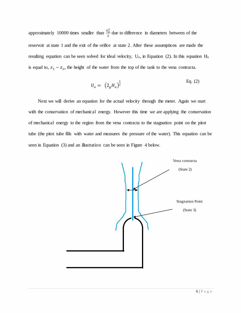
Next we will derive an equation for the actual velocity through the meter. Again we start
with the conservation of mechanical energy. However this time we are applying the conservation
of mechanical energy to the region from the vena contracta to the stagnation point on the pitot
tube (the pitot tube fills with water and measures the pressure of the water). This equation can be
seen in Equation (3) and an illustration can be seen in Figure 4 below.
Eq. (2)
Vena contracta
(State 2)
Stagnation Point
(State 3)

7 | P a g e
Figure 4: An illustration of the water flow from the vena contracta around the pitot tube
𝑃2
𝜌+
𝑈22
2+ 𝑔𝑧2 =
𝑃3
𝜌+
𝑈32
2+ 𝑔𝑧3 + 𝑔ℎ𝐿
Once again we have to make some assumptions for the equation to match our experiment.
First we assume that 𝑧2 is equal to 𝑧3 because the location of 2 and state 3 are relatively equal
when compared to the size of our experiment. Next we assume that 𝑔ℎ𝐿 is equal to zero because
the distance is short and it is inside a free jet. The last assumption we make is that U3 is equal to
zero because it is at the stagnation point of the Pitot tube. After making these assumptions and
solving for the actual speed, U2, the resulting equation can be seen below.
𝑈2 = (2
𝜌(𝑃3 − 𝑃2))
12
If you expand on equation 4 and set P3 equal to Patm plus 𝜌𝑔𝐻𝑐 and assume P2 equals Patm we
find the following equation. Hc is the water level in the Pitot tube measured from the stagnation
point. This is illustrated in Figure 3.
𝑈2 = (2
𝜌(𝑃𝑎𝑡𝑚 + 𝜌𝑔𝐻𝑐 − 𝑃𝑎𝑡𝑚))
12
This the expansion allows for us to simplify the actual speed equation into the following.
𝑈2 = (2𝑔𝐻𝑐) 12
Using the ideal velocity and the actual velocity, Equations (2) and (6), we can form a
coefficient of velocity which can be seen below in Equation (7).
Eq. (3)
Eq. (4)
Eq. (5)
Eq. (6)

8 | P a g e
𝐶𝑈 = (𝑈𝐶
𝑈𝑜
) = (2𝑔𝐻𝑐
2𝑔𝐻𝑜
) 12
Next we will derive a coefficient of contraction which will relate the actual area of water
flowing through the orifice, ac, to the ideal area of the orifice, ao. This is seen below in Equation
(8).
𝐶𝐶 = (𝑎𝐶
𝑎𝑜
)
To calculate ac and ao we use the area of a circle 𝑎 = 𝜋
4𝑑2. This can be seen plugged into
Equation (8) below.
𝐶𝐶 = (
𝜋4
𝑑𝑐2
𝜋4 𝑑𝑜
2)
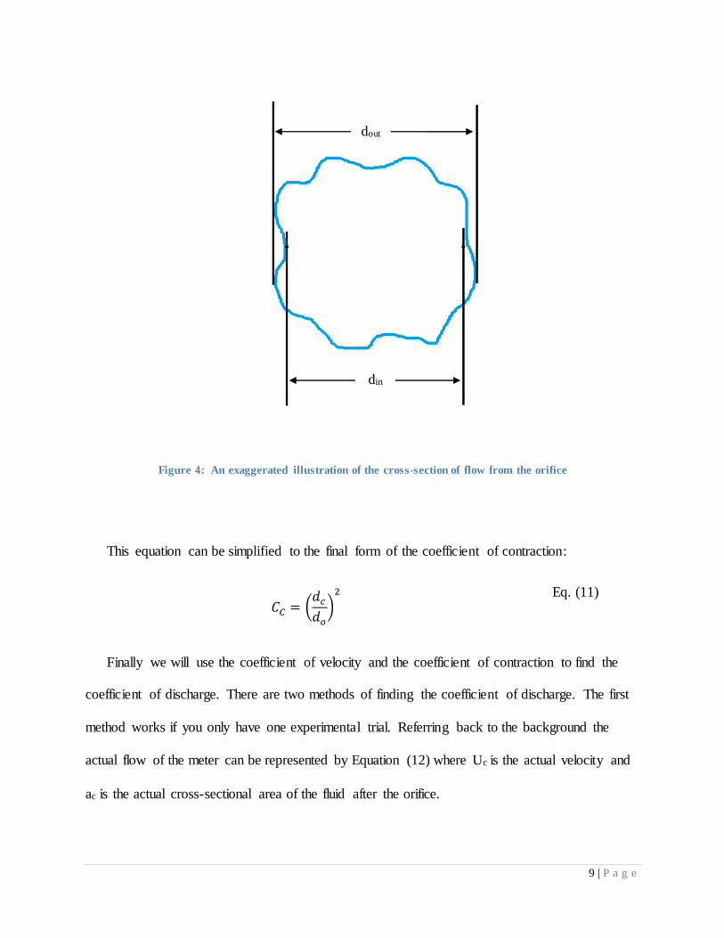
In this equation do is the ideal of the flow which is the diameter of the orifice and dc is the
actual diameter of the flow of fluid. The actual diameter can be calculated using the Equation
(10) where dout and din are defined in Figure 5.
𝑑𝐶 = (𝑑𝑜𝑢𝑡 + 𝑑𝑖𝑛
2)
Eq. (7)
Eq. (8)
Eq. (9)
Eq. (10)
9 | P a g e
Figure 4: An exaggerated illustration of the cross-section of flow from the orifice
This equation can be simplified to the final form of the coefficient of contraction:
𝐶𝐶 = (𝑑𝑐
𝑑𝑜
)2
Finally we will use the coefficient of velocity and the coefficient of contraction to find the
coefficient of discharge. There are two methods of finding the coefficient of discharge. The first
method works if you only have one experimental trial. Referring back to the background the
actual flow of the meter can be represented by Equation (12) where Uc is the actual velocity and
ac is the actual cross-sectional area of the fluid after the orifice.
Eq. (11)
dout
din

10 | P a g e
𝑄𝑎𝑐𝑡 = 𝑈𝑐𝑎𝑐
Using our coefficient of velocity and contraction we now know 𝑈𝑐 and 𝑎𝑐. This substitution
can be seen below.
𝑄𝑎𝑐𝑡 = 𝐶𝑈𝑈𝑜𝐶𝑐𝑎𝑜
As we know from the background 𝑈𝑜 𝑎𝑜 is the ideal flow of the meter and Qact is the actual
flow measured in the experiment. This leaves us with the coefficient of discharge, CD.
𝐶𝐷 = 𝐶𝑈𝐶𝐶
Method 2 for finding the coefficient of discharge is a representative value for a range flows.
For this method we start with a similar equation (see Equation (15)) but we define the velocity
differently as seen in Equation (16).
𝑄𝑎𝑐𝑡 = 𝐶𝐷𝑄𝑖𝑑𝑒𝑎𝑙 = 𝐶𝐷𝑈𝑜 𝑎𝑜
𝑄𝑎𝑐𝑡 = 𝐶𝐷𝑎𝑜(2𝑔𝐻0)1
2
Solving for CD gives us the coefficient of discharge using method 2.
𝐶𝐷 = 𝑀
𝑎𝑜(2𝑔𝐻0 )12
Eq. (12)
Eq. (13)
Eq. (14)
Eq. (15)
Eq. (16)
Eq. (17)

11 | P a g e
Experimental Method
As seen below in Figure 5 the orifice meter that we used in our lab was vertically positioned.
In order to determine the discharge coefficient of our meter we recorded the Ho and Hc values for
eight different flow rates (Q) through the meter. The Ho and Hc values were recorded using the
piezometer tubes on the side of the meter seen in Figure 5. The flow rates were measured by
recording the time it took to fill a fixed 15 liters of water.
Figure 5: The orifice meter used in our experiment
Piezometer tubes
(Hc on the left, Ho on the right)

12 | P a g e
Before any data can be recorded the orifice meter must be balanced on the top of the fluids
bench. This can be done by adjusting the tripod legs of the meter. Next all of the connections
should be checked and made secure. There should be a connection from the bench supply valve
to the sprinkler pipe, from the collecting hopper to the weighing tank and from the overflow pipe
to the waste hole in the bench.
In the first part of the experiment we measured CD, Cu, and Cc with a constant value of Ho. In
the second part of the experiment only the CD value was measured but for a number of different
values of Ho. The Cu and Cc are assumed to be constant throughout the experiment of changing
Ho values. For the first part described above the water level was filled in the orifice meter to the
height of the overflow pipe and the inflow of the meter should be regulated so a small steady
discharge is obtained from the overflow pipe. This will ensure that the level in the tank remains
steady while the measurements are being made. The CD value can be calculated from the
recording the time it takes to fill the fixed value of 15 liters of water in the tank and recording the
value Ho. In order to measure the coefficient of velocity (Cu) the Pitot tube is centered in the
emerging jet as close to the tank as the meter will allow. (The Pitot tube assembly can be seen
below in Figure 6). This will allow the meter to measure at the vena contracta. The values of Ho
and Hc should be recorded. Next to measure the coefficient of contraction (Cc) it is necessary to
find the diameter of the jet at the vena contracta. As described in the analytical method this needs
to be an average diameter of the jet by measuring dout and din. This is done using the blade on the
Pitot tube assembly. The blade is placed and the level of the vena contracta and brought to one
side of the jet. As seen in Figure 6 there is a measurement dial that controls the horizontal
movement of the blade. Note the position of the dial when it is on one edge of the jet. For the
outer diameter the blade should then be brought through the jet to the other side noting how far

13 | P a g e
the blade moved using the scale on the dial. (One full turn equals 1 mm of movement.) To
measure the inner diameter, the blade is moved into the edge of the jet until the water just begins
to cover the whole blade. The blade position is noted and moved to the same position on the
opposite side of the jet. The total distanced the blade moved should be recorded as din.
Figure 6: A close up of the orifice and Pitot tube assembly
Next we can move on to the second part of the lab experiment. For our lab we took a total of
eight measurements of different Ho values. The Ho values were chosen to be evenly distributed
Measurement
Dial
Pitot tube
Blade
Vena Contracta

14 | P a g e
across the total height of our piezometer tubes. Care should be taken to allow the water level to
settle to a steady value after the inflow to the tank has been changed. Once the level has settled
the Ho value should be recorded and the tank can be filled to a volume of 15 liters. The tank
volume scale is located on the side of the fluids bench and can be seen in Figure 7. Once filled
the time elapsed should be recorded. It should be noted that the Ho may vary during the time
interval and this vary should be noted for uncertainty purposes. This procedure should then be
repeated for all eight tests.
Figure 7: An image of the Tank volume scale
All of the measurements taken using methods above have associated sources of random and
systematic error except for the tank volume measurement. The tank volume scale was taken as
true and we did not account for any error in the measurement. Random error occurs from
phenomenon such as common human error in reading a scale and jitter in a meter. Systematic

15 | P a g e
error is consistent with the tool of measurement and results from the resolutions of the device
and manufacture data. All of the uncertainties associated with measurements taken in this lab can
be seen below in Table 1.
Device Measurement Symbol Units Random
Uncertainty
Random
Uncertainty
Total
Uncertainty
(95%)
Timex Wrist
Watch
Time t s 0.1 0.01 0.1
Piezometer
Tubes
Piezometer
height
Ho,Hc mm 5 .5 5
Blade
Adjustment
Dial
Jet diameter Dc mm 0.1 0.05 0.1
Table 1: A table of Uncertainties for measured values
Results
Test 1 2 3 4 5 6 7 8
Volume of water (L) 15 15 15 15 15 15 15 15 Time (s) 61.65 64.15 66.97 71.1 75.51 81.41 86.06 95.18
Head on orifice, Ho (mm) 386 350 326 289 250 218 187 153
Pitot Tube Reading Hc (mm) 386
Inner Diameter (mm) 9.8
Outer Diameter (mm) 12
Diameter of vena Contracta, Dc (mm) 10.7
(Ho)1/2 (m1/2) 0.621289 0.591608 0.570964 0.537587 0.5 0.466905 0.432435 0.391152
104 x Q (m3/s) 2.43309 2.33827 2.239809 2.109705 1.986492 1.842525 1.74297 1.575961
Cu 1
Cc 0.795
Method 1 CD 0.795
Method 2 CD 0.745
Table 2: A table summarizing lab Data

16 | P a g e
Table 2 shows all data that was measured and calculated after performing the lab experiment.
Equations used and sample calculations can be seen in Appendix A. Explanation of each
equation can be seen in the Analytical Method section of the report. The slope (m) that was used
in Equation (17) was taken from the plot Figure 8 below which shows the relationship between
the piezometer tube height and the volumetric flow rate.
Figure 8: A standardized plot of flow rate vs Ho values
y = 3.7287x + 0.1171
R² = 0.9986
0
0.5
1
1.5
2
2.5
3
0 0.1 0.2 0.3 0.4 0.5 0.6 0.7
10
4x
Q (
m3/s
)
(Ho)1/2 (m1/2)
Q x 104 vs Ho1/2

17 | P a g e
Value Units Calculated
Result
Systematic
Uncertainty
Random
Uncertainty
Total
Uncertainty
dc mm 10.7 0.05 .01 0.1
Hc,Ho mm 386 0.5 5 5
Cu n/a 1 0.25 2.5 2.5
Cc n/a 0.795 0.01117 0.02233 0.025
CD Method 1 n/a 0.795 0.2003 1.988 1.2
m 𝑚52
𝑠
3.7287 n/a n/a 0.01198
CD Method 2 n/a 0.745 n/a n/a 0.12
Table 3: A table of uncertainties for calculated results
Above in Table 3 the uncertainties can be found for each of the calculated results in this lab
experiment. Detailed calculations of uncertainties can be found in Appendix B. It should be
noted that the uncertainty value for the coefficient of discharge that was calculated for method 1
is not a reasonable value. This may be due to an error in the calculations or simply due to the
high uncertainty value measured in the piezometer tubes that was amplified through the
calculations. The slope and method 2 for solving do not have coefficient of discharge do not
have systematic or random error.
Discussion and Conclusion
In order to determine if the calculated values for the coefficient of discharge for our meter
were reasonable we can compare our values with the value calculated in the lab handout. With
our 95% confidence interval we can conclude that our method 1 value of CD (0.795 ± 1.998)

18 | P a g e
would agree with the given value from the lab handout of 0.63. It should be noted that the
calculated uncertainty value for method 1 is much too large to reasonable. This could be due to
an error in calculations in Appendix B.
Another aspect of our results that we can discuss is the linearity of Figure 8 which plots the
relationship of Ho values to the volumetric flow rate of the meter. The linearity of the line can be
reviewed using the coefficient of determination (R2). This value is shown in Figure 8 and can be
calculated easily in Excel. Our R2 value turned out to be 0.9986 which proves our data to be
almost perfectly linear (R2 = 1).

19 | P a g e
References
1. Orifice Meter Parameters. (n.d.). Retrieved February 17, 2015, from
http://www.engineeringexcelspreadsheets.com/wp-content/uploads/2011/04/Orifice-
Meter-Parameters.jpg
2. Vena Contracta. (n.d.). Retrieved February 17, 2015, from
http://upload.wikimedia.org/wikipedia/common
3. Munson, B., & Okiishi, T. (2013). Fundamentals of Fluid Mechanics (7th ed.).
Hoboken, NJ: J. Wiley & Sons.
4. Orifice, Nozzle and Venturi Flow Rate Meters. (n.d.). Retrieved February 17, 2015,
from http://www.engineeringtoolbox.com/orifice-nozzle-venturi-d_590.html


![Furukawa LAB. · 2020. 6. 15. · Furukawa LAB. [Nonlinear and nonequilibrium phenomena in complex fluids] Department of Fundamental Engineering. Physics of Complex Fluids. Department](https://static.documents.pub/doc/80x56/6065e202fa00d50a91418119/furukawa-lab-2020-6-15-furukawa-lab-nonlinear-and-nonequilibrium-phenomena.jpg)


