luorescence correlation spectroscopy �FCS� has at-racted considerable attention in many domains ofcience.1–4 FCS, which was initially introduced forhe study of chemical kinetics,5 later was used toeasure several molecular parameters1–4; thus it is
ot surprising that the remarkable advantages ofCS have been recognized and utilized in physics,ngineering, chemistry, biology, medicine, and theirnterdisciplinary contexts.
The versatility of FCS methods stems from the facthat fluorescence and its fluctuations can easily benduced and detected in a wide range of experimentalonditions, as has been encouraged by the use of aingle laser beam in conjunction with efficient fast pho-odetectors and modern electronic correlators. Butersatility and sensitivity to many molecular parame-ers are not the sole rewarding qualities of FCS. Theechnique has also proved suitable for single-molecularetection in gases, liquids, and condensed matter.everal authors have indeed reported that microscopynd proper laser characterization can be combined to
The author �[email protected]� is with the Enteer le Nuove Tecnologie, l’Energia e l’Ambiente, Casaccia, Vianguillarese 301, 00060 S. M. di Galeria �Rome�, Italy.Received 4 February 2004; revised manuscript received 16 June
timulate many studies and applications in whichingle-molecule detection plays a key role.1–4 Amonghese studies, FCS methods applied to observation ofingle fluorophores in aqueous media at room temper-ture are of particular interest.1–4,6–11 The study iseing conducted within biophysical and biochemicalnvestigations, which are becoming increasingly valu-ble in the development of accurate biotechnologiespplied to medical science. For this reason, in theest of the paper we refer mainly to fluorescence asbtained from sparse molecules in liquid solutions.The conceptual elements of FCS are simple andere borrowed from the optical version of correlation
echniques used for the study of the degree of coher-nce of light sources.12,13 In the context of low levelsf dilution, a correlation measurement is performedith a focused laser beam that provides the excitingnergy absorbed by the sample. Induced fluores-ence F�t� fluctuates with time t because the radiat-ng molecules within the liquid experience changeshat have several causes �diffusion, flow motion,hemistry, laser-induced phenomena, and so on�.he resultant fluctuations �F�t� � F�t� � �F�t� of
ime average �F�t� carry information on the interac-ions that generate the observed variations in thenduced optical response. More specifically, this in-ormation is stored in the shape of the intensity cor-elation:
nd one usually retrieves it by relying on the well-nown three-dimensional Gaussian �3DG� approxi-ation,14 which simplifies the algebra involved in the
olution of Eq. �1�.In this type of measurement it is of utmost impor-
ance that the probe volume remain well character-zed. This volume is described by spatialistribution ��r� of the observed fluorescence andarticipates in the interpretation of �F�t� in terms ofocal fluctuations �C�r, t� of molecular concentration;hat is,
�F�t� � F�t� � �F � k � �C�r, t���r�dr, (2)
here k is a constant that accounts for absorptionross section, quantum yield, collection, and detectorfficiency. With the help of Eq. �2�, correlation func-ion G�� is more explicitly given by
G�� ��� ��C�r, t � ��C�r , t���r���r �drdr
� �C � ��r�dr�2 ,
(3)
nd, for example, the average molecular concentra-ion �C can be determined from correlation ampli-ude G�0� � 1��CVeff, where Veff is the effectiveeasurement volume, defined by
Veff � �� ��r�dr�2�� �2�r�dr . (4)
rom this cursory review, which one can find amplifiedn more-extensive publications on the subject,2,4–8,11,14
t is clear that the understanding of FCS measure-ents strongly depends on the probe volume de-
cribed by the function ��r�, which enters into all theelevant expressions summarized in Eqs. �2�–�4�.ut what happens if this volume undergoes somenpredicted changes? Neither the fluorescence rateor the correlation function is well defined, and quan-itative interpretation becomes unreliable. Such aroblem, which is often recognized in fluorescenceeasurements,15–24 originates from the interplay be-
ween uneven spatial distributions of laser beamsnd molecular saturation. Inasmuch as the probeolume is determined by the actual distribution ��r�f fluorescent molecules, it is intuitive that moleculesn the spatial peak of the laser beam are likely toxperience strong saturation and consequently tendo flatten ��r�, whereas increasing numbers of mole-ules, situated in the tails of the spatial laser profile,ontinue to broaden spatial emission ��r� for increas-ng laser intensity. This means that the probe vol-me widens as the laser intensity increases and thathe correlation decreases accordingly. It is thus un-erstood that a reliable description of such probe vol-me effects is crucial in FCS spectroscopy, and in this
aper I intend to make a significant contribution tohe scientific discussion of the subject.
The paper is organized as follows: The standardpproach to FCS measurements �i.e., without probeolume effects� is briefly reviewed in Section 2.nown corrections to standard FCS are then consid-red in Section 3 as an introduction for the reader tohe original contribution of this work, which is set outn Section 4. The theoretical treatments of averageuorescence �F, spatial emission ��r�, and purelyiffusive correlation are reported in the subsectionsf Section 4. Final conclusions are given in Section. To help the reader to find his or her way throughome important stages of the calculation, some keyesults of this paper are given in Appendix A.
. Standard Theory
he conceptual basis of FCS for liquid solutions atow levels of dilution is rather simple and can beound in a number of publications.1,2,4 In this paper,owever, the theory for monodisperse molecules areriefly reviewed to permit immediate comparisonith the results presented in the following sections,
n which modifications are laid out.Consider then a laser of intensity I0 and spatial
rofile I�r�, which excites a group of sparse moleculesf average concentration �C. As anticipated above,patial changes in the induced fluorescence are de-cribed by the function ��r�, which combines the so-alled collection efficiency function CEF�r� andxcitation profile E�r�:
��r� � CEF�r�E�r�, (5)
ith E�r� � In�r� �n � 1 for one-photon excitationOPE�, n � 2 for two-photon excitation �TPE�, and son�, and function CEF�r� describes the spatialhanges in the detected light emitted by a pointource and observed through a pinhole located in theicroscope image plane.Equations �2�–�5� can all potentially be carried
hrough once the spatial profile of laser intensity I�r�as been specified. The choice of a Gaussian–orentzian �GL� beam1 is by far the most importantecause reproduces the actual shape of laser beamsmployed in FCS.2 Then
I�r� � I0
exp��2r2�w2� z��
1 � � z�z0�2 , (6)
here r � �r, z� with r the radius in the �x, y� planeerpendicular to laser propagation axis z, and w2�z�w0
2�1 � �z�z0�2� with w0 the beam waist and z0 theonfocal parameter. In this case it is straightfor-ard to give the spatial dependence of emission:
�GL�r, z� � I0nCEF�r, z�
exp��2nr2�w2� z��
�1 � � z�z0�2�n , (7)
hich can be used in the calculation of Eq. �3�. Butt can be readily understood that �GL does not permitn easy theoretical treatment of correlation func-ions. First, the laser profile in Eq. �6� introduces a
Lstsrfiti
Epasfi
Atfjwu
tacaotomatfG�p
tb
wb
wfae
w�iI
ttwpnct
wGKs
dtaiecwbf
icirfeabdvrlbtaarua
3C
Tftfisisip
orentzian dependence of difficult integration, and,econd, CEF�r, z� has to be described by Fourier op-ics,25 where the point-spread function of the micro-cope objective is convoluted with the function thatepresents the pinhole. As a result, the correlationunction cannot be solved analytically with �GL. Its then common practice to resort to 3DG approxima-ion,14 in which the laser beam in Eq. �6� is turnednto a pure 3DG function:
I�r, z� � I3DG�r, z� � I0 exp��2�r2�w02 � z2�z1
2��. (8)
quation �8� removes the untreatable Lorentzian de-endence of Eq. �6�; if, additionally, small pinholesre not used in the setup such that CEF�r, z� does notignificantly alter the relevant extension of laser pro-le, the emission function �GL is approximated by
�GL�r, z� � �3DG�r, z� � I0n exp��2n�r2�w0
2 � z2�z12��.
(9)
s will be shown below, relations �8� and �9� simplifyhe algebra involved in the correlation of purely dif-usive dynamics. Note, however, that relation �9� isust a consequence of relation �8� for TPE setups forhich pinholes are not used and CEF�r, z� is set tonity.The 3DG approximation is empirically justified by
he weak dependence of correlation on the axial vari-ble �i.e., z coordinate�, and therefore proper modifi-ations of functional dependences on that variablere of minor effect. Moreover, confocal parameter z0f real focused laser beams is significantly greaterhan beam waist w0, and thus the relevant time scalef diffusive correlation is given mainly by the para-etric dependence on w0 �which is not altered in the
pproximation�. As a final comment, let us noticehat parameter z1 in relation �9� might be differentrom z0 in Eq. �6� to consider the fact that axialaussian wings in approximate emission function3DG should be adjusted to match better the actualrobe volume described by �GL.Correlation function GD�� of the fluorescence fluc-
uations of diffusing particles can now be calculated,ecause it is known that for Brownian motion
��C�r, t � ��C�r , t� � �C�4�D��3�2
� exp���r � r �2�4�D�,
(10)
here D is the diffusion coefficient. Equation �3�ecomes
GD�� � GD�0�1
1 � �D
1�1 � �w0�z1�
2�D�1�2 , (11)
here characteristic decay time D is related to dif-usion coefficient D according to D � w0
2��4nD� andmplitude GD�0� is inversely proportional to the av-rage number of molecules �N:
G �0� � 1��N, (12)
D
20
ith �N � Veff�C and Veff � 23�2V3DG � ���n�3�2w02z1
volume V3DG � ���2n�3�2w02z1 is defined by spatial
ntegration of normalized emission function �3DG�0
n�.Apparently Eqs. �11� and �12� provide an easy in-
erpretation of diffusion, but the outcome of correla-ion experiments is much more complex than whatas reported above. Other effects, caused by photo-hysical processes, must be considered. Fortu-ately enough, the other relevant effects are fastompared with diffusion, and their contributions tohe general expression of G�� can be factorized:
G�� � GD����� � K, (13)
here function ��� summarizes the component of�� that results from intramolecular dynamics andis a constant relative to the background that in
ome cases might be nonnegligible.26
The meaningful contributions to ��� might be of aifferent nature. For example, photobleaching andriplet-state kinetics are often considered,15,17,18,20,22,24
nd suitable expressions for G�� have been found tonterpret experimental data. In this manner the av-rage number �N of molecules and diffusion time Dan be retrieved from diffusive correlation GD��,hereas other molecular parameters, such as photo-leaching and intersystem crossing rates, are obtainedrom the remaining decay, ���.
For the purposes of this paper we are not interestedn the explicit form of G�� except for its diffusiveomponent, for which the effect of excitation volumes crucial. The need for a detailed description of theole of diffusion in FCS measurements can be seenrom Eq. �13�. The specific forms of this equation arextremely useful for recovery of detailed informationbout molecular dynamics. But, if diffusive contri-ution here differs from GD�� as obtained in stan-ard theory, then fitting models applied to measuredalues of G�� will have a weakened ability to extracteliable parameters from both GD�� and ���. Theikelihood that such a problem will occur is magnifiedy the large number of parameters that are allowedo vary freely in fitting procedures �for instance, therere eight free parameters in Eq. �34� of Ref. 17�. Asconsequence, a general expression of diffusive cor-
elation, including saturation-modified probe vol-mes, is advisable to minimize uncertainties in data-nalysis routines.
. Probe Volume Corrections in Fluorescenceorrelation Spectroscopy
he sensitivity of fitting procedures to deviationsrom the diffusive factor of Eq. �13� is not a specula-ive consideration, because it has been clearly af-rmed in experiments in which typical OPE and TPEetups have been employed.17,24 Hence a better def-nition of saturation and probe volume effects in FCSeems to be one of the major advances to enhance thenterpretation of experimental outcomes. Actually,revious authors have tried to get at this issue and,
efore proceeding further, it is important to brieflyecap their major conclusions.
A thorough investigation of the intramolecular dy-amics within the context of OPE FCS of fluoro-hores in solutions is found in the research ofidengren et al.17 They have clearly pointed out
hat high excitation intensities, used to increase sig-al�noise ratios, can induce significant distortions inhe spatial distribution of emitted fluorescence.evertheless a detailed analysis has been developed
nly for the photodynamic aspects of FCS measure-ents at high excitation intensities. The alteration
xpected in the diffusive component of measured cor-elation decays has been limited to an additional cor-ection term that was assumed to be a replica oftandard theory �Eq. �11��. In symbols, theaturation-corrected diffusive correlation was as-umed to be given by
here the subscript WMR is the initials of the au-hors of Ref. 17. From Eq. �14� it is clear that thewo diffusion times 1D and 2D are necessary to com-ensate for the measured deviation from Eq. �11�nasmuch as a second diffusion time improves theontrol on the time scale of correlation decays. Pa-ameter A in Eq. �14�, which ranges from 0 to 1,ssigns an amplitude to distinguish the weight of thewo standard terms of GWMR��. With this change inhe diffusive correlation, those authors17 found thatheir data could be better fitted, and therefore Eq.11� was discarded. However, the explanation of Eq.14� is of a qualitative nature only and refers to annspecified influence of the spatial laser wings atigh laser intensities. In reality, Eq. �14� is open toriticism. First, there is neither physical nor math-matical support for a requirement that the correc-ion term be formally equal to the standard resultiven in Eq. �11�. Second, the additional diffusionime adds another molecular parameter of difficultnterpretation, as if two competing diffusion pro-esses took place at the same time, one with timecale 1D and the other with time scale 2D. Third,he increase in the number of fitting parametersthere are eight in the mentioned example of Ref. 17�educes confidence in the fitting routines, especiallyhen some of the parameters do not have a realhysical origin.Attempts at understanding probe volume effects in
CS have been made for TPE FCS also. For in-tance, Mertz reported discrepancies between predic-ions and experiments in TPE fluorescenceicroscopy.20 In a standard approach �Section 2� it
s obvious that fluorescence scales with the square ofaser intensity I0 �relation �9��, but large deviationsre reported in Mertz’s work �see, for example, Fig. 9
f Ref. 20�. Initially, it was assumed that a modelncluding saturation, intersystem crossing, and lin-ar photobleaching could provide the correct physicalase with which to explain the observed deviations,ut this model was insufficient. It was thought thatigh-order photobleaching processes could have hadrole in the measurements, but the assumption wasot enough to permit the data to be interpreted, andhus the occurrence of other photophysical processesas qualitatively hypothesized.Recently the role of excitation saturation in TPE
CS was examined in more detail by Berland andhen �BS�.24 They investigated ways in which thetandard diffusive contribution to the correlationunction may be modified by saturation broadening ofhe probe volume. The key idea of the research ofS lies in a mathematical ability to conceptualize thepatial distribution of fluorescence as a combination
f two Gaussian functions such that their differencequals the actual emission volume �Eq. �7� and Fig. 3f Ref. 24�:
�BS�r, z� � I02 exp��4�r2�w0
2 � z2�z12��
� Is2 exp��4�r2�ws
2 � z2�zs2��. (15)
he Gaussian origin is simply due to the 3DG ap-roximation �relation �8��, whereas the difference be-ween the two Gaussian functions is worked out from3DG�r, z� in relation �9� and a fictitious Gaussianaturated profile �s�r, z� � Is
2 exp��4�r2�ws2 � z2�zs
2��,hich represents the subtracted function needed to
imulate the real saturated spatial emission. Inten-ity parameter Is � �I0
2 � Ith2�1�2 �where Ith defines
he laser saturation threshold� and the other spatialarameters ws and zs of the fictitious Gaussian profilere obtained under the constraint that the differenceetween �3DG�r, z� and �s�r, z� given in Eq. �15� pro-uce the saturated top-hat spatial profile. This con-traint is formally expressed by the followingelationships:
� �Is
2
I02 �
ws2
w02 �
zs2
z02 �
I02 � Ith
2
I02 , (16)
here � is a dimensionless variable that defines theegree of saturation for I0 � Ith. In the oppositeange, I0 � Ith, Eqs. �15� and �16� are no longer valid,nd the standard theory of Section 2 is assumed toold. Based on these assumptions, the calculations
ead to the average fluorescence rate �F:
�F � � k�CI02V3DG I0 � Ith
k�CI02V3DG�1 � �5�2� I0 � Ith
, (17)
nd to the diffusive correlation for I � I :
2 � �1 � A�1
1 � �2D
1�1 � �w0�z1�
2�2D�1�2� , (14)
1D�1�
0 th
Ii
paptmhammrwcptpfprbadPtdssot
dsbesl
4
Itmtrtqlve
tt
blww
wttt�ddiMupswts
A
Tsr�cc�oaeoWaoevospi
aanhrws
n the limit of I0 � Ith, standard correlation functionn Eq. �11� was assumed to be true.
Although the model has produced some small im-rovements, Berland and Shen found large discrep-ncies in fluorescence measurements at high laserowers. The source of this disagreement was iden-ified as the inability of the proposed saturationodel to reproduce the actual volume observed at
igh laser intensities. Nonetheless, predictionsbout photobleaching have also been carried out fromeasured correlation decays, but the limitationsentioned above made it difficult to justify an accu-
ate elaboration of data acquired with laser powersell above saturation threshold. Apart from the in-
onvenience that Berland and Shen highlighted, theroposed model has some other drawbacks. First,here is no physical meaning behind the saturatedrofile �s�r, z�. This profile is just a clever expedientor finding a mathematical tool with which to ap-roach the problem, but it introduces fictitious pa-ameters Is, ws, and zs that do not belong to a realeam. Second, the abrupt change between standardnd saturated behavior, represented by the two con-itions I0 � Ith and I0 � Ith, appears unphysical.robe volume effects and saturation are instead con-
inuous phenomena. In particular, conventional un-erstanding of fluorescence saturation never includesuch a sudden change at I0 � Ith.1,13,16 The onset ofaturation is indeed expected well below the thresh-ld limit, and, correspondingly, a physically basedheory should exhibit this feature.
All in all, the issue of probe volume effects in theiffusive component of fluorescence correlation seemstill far from being understood and it is clear that aetter comprehension of it would be important forstablishing reliable criteria for quantitative mea-urements in FCS and fluorescence microscopy atarge.
. New Approach to Probe Volume Effects
n FCS spectroscopy the problem of dealing with spa-ial inhomogeneities of laser beams can be solved in aore elegant way within the 3DG approximation es-
ablished in relation �8�. The further assumption inelation �9� of negligible influence of pinhole aper-ures remains valid here. So we are left with theuestion of what emission function � can replace re-ation �9� of standard theory to account for probeolume effects without resorting to unphysical mod-ls.In carrying out the transition from relation �9� to
he new emission function, we use a recent opticalheorem that has been employed to analyze the time
GBS�� �GD�0�
�1 � �5�2�2 � 1�1 � �D��1 � �w0�z
�42�
�1 � 1�� � 2��D��1 � 1�� �
20
ehavior of saturated fluorescence signals.27 Its va-idity can be extended to average signals �F, and,ith the same notation as above, this theorem can beritten as follows:
d�F
dI0�
�k�Cw02
2I0 ��zinf
zsup
��0, z�dz, (19)
here zinf and zsup denote the generic interval of in-egration over the laser propagation axis. The rela-ionship between total fluorescence signals �F andheir component ��0, z� emitted from the center linei.e., the line traced by the spatial laser peak andefined by r � 0� is of fundamental importance for theevelopment of our approach, and, for completeness,ts mathematical proof is given in Appendix A.
ore, specifically, Eq. �19� is used initially to explainnusual deviations found in fluorescence microsco-y.20,24 Subsequent to this first achievement, aaturation-corrected emission function is obtainedith which to calculate the diffusive correlation func-
ion, which represents the main objective of thistudy.
. Fluorescence
he calculation of saturation-corrected correlationtarts with the derivation of the time-averaged fluo-escence �F that appears in the denominator of Eq.1�. Although it might seem like a secondary taskompared with the main focus on the importanthanges in the correlation function, the calculation ofF addresses two important questions in the devel-pment of our issue. First, it would be highly desir-ble that the new saturation model be capable ofxplaining some unclear experimental data thatther models failed to interpret �Section 3�.20,24
ith a positive answer to the first inquiry, we arellowed to tackle the problem of a reliable expressionf emission function �, which is at the core of thentire calculation. Note that this approach is in re-erse order from that of Ref. 24, in which the proposalf emission function �BS is initially set out. Ourtrategy, however, presumes that only a credible ex-ression of �F enables us to ascertain a correspond-ng emission function � to be used in Eq. �1� or �3�.
The primary concern is then to find the appropriateverage fluorescence �F that incorporates saturationnd associated probe volume effects. Unfortu-ately, the classic picture of FCS �Section 2� is notelpful, because assumes that �F � I0
n, and satu-ated volume distortions that are due to spatial laserings are not contemplated. But the problem can be
olved if we work out two simple solutions of Eq. �19�
n the limits of low and high laser intensities I0. Inhe lower limit, standard theory is applicable andocal fluorescence emission � must obey the power-aw dependence, i.e., ��0, z� � I0
n. It is then nourprise that Eq. �19� yields the same power law �F
I0n that is expected in standard theory. In the
pposite limit of very high I0, local signal ��0, z� isully saturated because is emitted from the spatialaser peak of relation �8�; therefore ��0, z� � ��,here �� is the constant saturated value. If this is
o, then Eq. �19� predicts that �F � log�I0�Ith�.ombining the two limit behaviors of �F yields theimplest solution:
�F � F0 log�1 � �I0�Ith�n�, (20)
ith F0 � ���2n�3�2k�Cw02z1Ith
n �see Appendix A.2or a detailed demonstration�. The noticeable ele-
ents that are different from the standard approachf Section 2 are two: the logarithm and Ith. Theogarithmic function stems from the resultant contri-ution to saturation of radial laser wings described byelation �8�, whereas the introduction of thresholdaser intensity Ith is necessary to preserve the dimen-ionless argument of the transcendental function.ut, apart from the mathematical need for Ith, itshysical meaning is evident from the conventionalnterpretation of fluorescence induced at high levelsf excitation.1,13,16 The threshold indeed marks theaser intensity at which saturation is a nonnegligibleeature; hence Ith is an important parameter to con-ider in FCS measurements. However, we do notnvestigate the detailed expression of Ith, as it in-olves the solution of intramolecular dynamics,hich lie outside the focus of this paper on corrections
o diffusive correlation, and, even though a more-recise interpretation can be retrieved from the lit-rature,1,13,16 Ith is treated as a free parameter.As a last comment on Eq. �20�, it must be said that
he logarithmic dependence of fluorescence satura-ion is not new in fluorescence spectroscopy.28,29
pecific calculations within the context of combustioniagnostics have already shown that for linear fluo-escence �n � 1� the logarithmic dependence is airect consequence of saturation induced by Gauss-an laser profiles, and, although this dependenceould have been given as a known fact, its derivations presented here to highlight the richness of infor-
ation contained in Eq. �19�.The saturation model established in Eqs. �19� and
20� can now be tested for experimental discrepanciesn fluorescence measurements. To that end, exper-ments carried out within TPE FCS offer importantpectroscopic examples to be mentioned. Thishoice is additionally dictated by the fact that TPECS has proved valuable for improving spatial reso-
ution and background suppression in comparisonith FCS based on one-photon excitation.22 TPECS is thus the correct candidate for finding out howood the proposed saturation model fits experimentalata available in the literature.
A first test is provided by the expected deviation Rrom the standard TPE FCS square dependence:
R �log�1 � �I0�Ith�
2�
�I0�Ith�2 . (21)
quation �21� is plotted in Fig. 1. Threshold Ith wasdjusted to reproduce the horizontal scale of Fig. 9 ofef. 20, where measured values of function R are
eported. From comparison of Eq. �21� with the ex-erimental values of R it is possible to assert that theroposed saturation model manages to predict whats observed in reality. The model suggested in Ref.0, however, in which, besides saturation, other dy-amic mechanisms such as intersystem crossing andhotobleaching were included, failed to explain thebserved behavior of R. As a solution, it was as-umed that other photophysical processes had beenecisive in the experimental result, but Eq. �21� hereroves that adequate evaluation of saturation is al-eady enough to explain much of the observed behav-or of R.
To strengthen the confidence in our model, addi-ional confirmation has been found in the paper oferland and Shen.24 Their Fig. 5 shows the com-arison between some experimental points and theesult of the BS saturation model, which was reca-itulated in Section 3. But, apart from the obviousgreement between theory and experiment in the lowange of laser powers, large inaccuracies are observ-ble for values of laser power that are relevant foraturation. Those authors recognized that theirodel is unable to describe the enlargement of the
robe volume observed at higher laser excitations,nd therefore their experimental findings still lackull explanation. In Fig. 2 of the present paper, Eq.20� is plotted as a continuous curve, and it is clearlyisible across the whole range of laser powers thathere is good agreement with the experimental dataf Fig. 5 of Ref. 24. The BS model, summarized inq. �17� and shown as a dashed curve in Fig. 2, fails
nstead to predict the observed fluorescence. Theain reason why Eq. �20� outperforms Eq. �17� is
ig. 1. Relative deviation R as obtained from Eq. �21�. The hor-zontal scale has been adjusted to match the horizontal scale of Fig.
of Ref. 20.
fpi
pttidnmmttlwtamsrI
BG
ASet�aisrd
ctIis
Tp�asmmLiptizb
Faa
ound in the physical adherence to the saturationrocess encoded in Eq. �19�, whereas the mathemat-cal approach contained in the BS model suffers from
ig. 2. Power dependence of the two-photon induced fluorescences predicted by standard theory, Ref. 24 �or Eq. �17� in this paper�,nd this work.
Stmidstt
dfmfmtBtaso4er�orsFa�fl
hysical vagueness. One example among many ishe role of saturation threshold Ith. It is sure that, athreshold, fluorescence saturation is already a prom-nent effect, and emission deviates from power-lawependence on laser intensity.1,13,16,27–29 These phe-omena are included in Eq. �19�, in complete agree-ent with the correct physical understanding ofolecular saturation. By contrast, the BS model
akes for granted that squared intensity profiles holdrue at threshold instead of assuming that the squareaw is the limit of vanishing laser intensities �i.e.,ell below threshold�. In other words, according to
he assumptions in the BS model, the paradoxicalnd sudden transition from no saturation to theodel suggested in Ref. 24 contradicts the fact that
aturation is a continuous phenomenon that al-eady takes place well below nominal thresholdth.1,13,16,27–29
. General Emission Function in the Three-Dimensionalaussian Approximation
lthough the standard approach of FCS, reviewed inection 2, can account for many of the diffusion prop-rties of molecules investigated at low laser intensi-ies, it does not include changes in emission function, nor does it indicate a way to include them. As waslready shown in Ref. 24, spatial alterations in � arenstead important because they are responsible for aignificant departure from the ordinary diffusive cor-elation of Eq. �11� with consequent misapplication ofata-fitting procedures. Because these changes are
20
ontrolled by the ratio I0�Ith, it is intuitive to expecthat a more-general � will involve a dependence on0�Ith. The intuition can be founded on mathemat-cal facts by combination of Eqs. �19� and �20�. Theolution is
�3DGsat�r, z� � I0
n exp��2n�r2�w02 � z2�z1
2��
1 � �I0�Ith�n exp��2nr2�w0
2�. (22)
he generality of this result is ensured by two mainieces of evidence: the retrieval of relation �9� for I0� Ith and the demonstration exemplified in Figs. 1nd 2. But there is another heuristic argument thatupports Eq. �22�. As was already pointed out, theeaning of the 3DG approximation consists in theodification of the axial dependence such that theorentzian shape of the laser beam is transformed
nto a Gaussian profile �relation �8��. The radial de-endence remains unaltered because it determineshe relevant time scale of diffusion. We can try tomport this idea into the general saturation law In�r,���1 � �I�r, z��Ith�n�.16 With I�r, z� given by the GLeam of Eq. �6�, the saturated-emission function is
uppose now that, according to the 3DG approxima-ion, the radial dynamics is what matters most in theolecular photophysics of diffusion, whereas the ax-
al dependence is less significant. In this case the zependence can be removed from Eq. �23� and re-tored as it is in standard theory, and, even thoughhis reasoning might seem too simplistic, it leads tohe same result as Eq. �22�.
Before �3DGsat�r, z� can be used to estimate the
iffusive correlation, it is interesting to investigateurther the compatibility between the 3DG approxi-ation and the probe volume effects encountered in �
unctions. Admittedly, this compatibility is of noatter in standard theory because the introduction of
he 3DG approximation is well justified �Fig. 3�.ut, when saturation threshold is reached �I0 � Ith�,
he probe volume becomes larger, with a flatter top,nd the standard picture is no longer valid. Thisituation is illustrated in Fig. 4, where a comparisonf emission functions for TPE FCS is given. Figure�a� represents the actual distribution of fluorescencexpected for a GL laser beam, and Figs. 4�b� and 4�c�eproduce the approximate functions, �3DG
sat�r, z�Eq. �22�� and �BS�r, z� �Eq. �15��; the latter is basedn the BS model.24 The three parts of the figure areather similar, even though �3DG
sat�r, z� seems toimulate better the broadening in the r direction ofig. 4�a�. But differences are more clearly manifests soon as excitation levels are set above thresholdFig. 5�. GL emission �GL
sat�r, z� in Fig. 5�a� is nowat across the z axis, whereas the radial width has
ncreased further. As for the approximated func-ions in Figs. 5�b� and 5�c�, it can readily be seen thathe relevant r dependence of �GL
sat�r, z� is well re-roduced by �3DG
sat�r, z�. This is a clear sign of goodompatibility between probe volume effects and 3DGpproximation. Conversely, �BS�r, z� predicts auch smaller radial width, and therefore the attempt
o use the BS model at high laser intensities isoomed to failure. Both approximated functions,owever, underestimate the flatness of �GL
sat�r, z�cross the axial axis. In principle, one could solvehis problem by letting parameter z1 vary freely to
xtend the axial wings of �3DGsat�r, z� and �BS�r, z�.
onetheless, for the diffusion issue the z dependenceoes not seem to be so crucial,14 and the effect of axialismatches is of secondary concern.
. Diffusive Correlation Function
he important elements needed for determining theeneral diffusive correlation within the 3DG approx-mation has been laid out; the formal calculation cane completed by solution of Eq. �3� with the help of
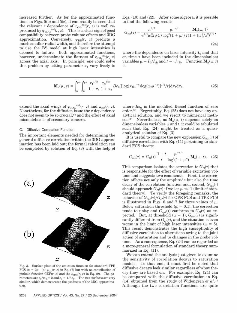
ig. 3. Surface plots of the emission function for standard TPECS �n � 2�: �a� �GL�r, z� in Eq. �7� but with no contribution ofinhole function CEF�r, z� and �b� �3DG�r, z� in Eq. �9�. The pa-ameters are z0�w0 � 2 and z1 � 1.7 z0. The two surfaces are veryimilar, which demonstrates the goodness of the 3DG approxima-ion.
qs. �10� and �22�. After some algebra, it is possibleo find the following result:
Gsat�� �n3�2
�3�2w02z1�C
��n�t
log2�1 � �n�
Mn��, t�t�1 � tw0
2�z12�1�2 ,
(24)
here the dependence on laser intensity I0 and thatn time have been included in the dimensionlessariables � � I0�Ith and t � �D. Function Mn��, t�s
here Be0 is the modified Bessel function of zerorder.30 Regrettably, Eq. �25� does not have any an-lytical solution, and we resort to numerical meth-ds.31 Nevertheless, as Mn��, t� depends solely onimensionless variables � and t, it could be tabulateduch that Eq. �24� might be treated as a quasi-nalytical solution of Eq. �3�.It is useful to compare the new expression Gsat�� of
iffusive correlation with Eq. �11� pertaining to stan-ard FCS theory:
Gsat�� � GD��1 � t
t��n�t
log2�1 � �n�Mn��, t�. (26)
his comparison isolates the correction to GD�� thats responsible for the effect of variable excitation vol-me and suggests two comments. First, the correc-ion affects not only the amplitude but also the timeecay of the correlation function and, second, Gsat��hould approach GD�� if we let � �� 1 �limit of stan-ard theory�. To verify the foregoing remarks, theehavior of Gsat���GD�� for OPE FCS and TPE FCSs illustrated in Figs. 6 and 7 for three values of �.elow saturation threshold �� � 0.1�, the correction
ends to unity and Gsat�� conforms to GD�� as ex-ected. But, at threshold �� � 1�, Gsat�� is signifi-antly different from GD��, and the situation is evenorse in the limit of high laser intensities �� � 5�.his result demonstrates the high susceptibility ofiffusive correlation to alterations owing to the jointction of saturation and to changes in the probe vol-me. As a consequence, Eq. �24� can be regarded asmore-general formulation of standard theory sum-arized in Eq. �11�.We can extend the analysis just given to examine
he sensitivity of correlation decays to saturationodels. To that end, it must first be noted that
iffusive decays look similar regardless of what the-ry they are based on. For example, Eq. �24� cane compared with the diffusive correlation in Eq.14� obtained from the study of Widengren et al.17
lthough the two correlation functions are quite
og� x1��n�log� x2�
�n��1�2�t�dx1dx2, (25)
e0��l
dbnpwltoetptFMrsucost
mdF
Gs4sc
F�from Fig. 3.
F�f
F1
ifferent in terms of their conceptual and physicalases, they can be very similar in terms of theirumerical behavior, as shown in Fig. 8. This im-lies that FCS measurements can be fitted equallyell with any saturation model, at the expense of
oss of confidence in existing fitting routines. Inhe example just mentioned, the reduced reliabilityf GWMR�� is immediately understood if one consid-rs that there are five different fitting parameterso manipulate �some of them do not have a realhysical meaning!� and, as a result, many combina-ions of those parameters are apt to duplicate inig. 8 the decay of Gsat�� at saturation threshold.ore generally, it is possible to conclude that the
etrieval of true physical parameters from mea-ured correlation values can be compromised bynphysical arbitrariness in the chosen diffusiveontribution to total correlation. In this regard,nly an approach that minimizes unphysical as-umptions can guarantee sufficient confidence inhe interpretation of FCS measurements.
As a further example of the importance of thisatter, we consider again the BS saturation model
escribed by Berland and Shen for TPE FCS.24 Inig. 9 the correlation functions G ��, G ��, and
D sat
20
BS�� �Eqs. �11�, �24�, and �18�, respectively� arehown for the same physical parameters as for Fig.. In apparent contradiction to what is expected ataturation threshold, the saturation-corrected BSorrelation coincides with standard correlation
ig. 4. Surface plots of �a� �GLsat�r, z�, �b� �3DG
sat�r, z�, and �c�
BS�r, z� for TPE FCS when I0 � Ith. The parameters are taken
ig. 5. Surface plots of �a� �GLsat�r, z�, �b� �3DG
sat�r, z�, and �c�
BS�r, z� for TPE FCS when I0 � 5Ith. The parameters are takenrom Fig. 3.
ig. 6. Gsat���GD�� as a function of t � �D for OPE FCS �n ��. Values of parameter � ��I �I � are shown.
D��. This is rather unusual because, by defini-ion, saturation cannot be negligible at thres-old,1,13,16,27–29 and one would expect a more-eneral correlation to converge to GD�� only wellelow threshold, as demonstrated by Figs. 6 and 7.he inconvenience associated with the use of GBS��
s the natural consequence of the unphysical basisssumed in the BS model. A more reasonable re-ult is instead given by Gsat��, which was obtainedollowing a precise physical model. As shownbove, these ambiguities between models can bettenuated if we change the values of some param-ters. In the example, Gsat�� approximates GBS��ith a much smaller saturation threshold than thatsed in Fig. 9 and, vice versa, GBS�� approachessat�� if substantial changes in amplitude and time
cale are included in GBS��.The findings that have been summarized above
ig. 8. Coincidence between Gsat�� in Eq. �24� and GWMR�� in Eq.14�. Standard correlation GD�� given in Eq. �11�, i.e., withoutorrections for volume effects, is shown as well for OPE FCS �n ��. The amplitude of GD�� was arbitrarily chosen and determineshe normalization of Gsat�� drawn for � � 1. One reaches theoincidence between Gsat�� and GWMR�� by varying the fittingarameters in GWMR��. Additionally, many combinations ofhese parameters are found to reproduce the behavior of G ��.
ndicate that the significance of fitting parametersepends strongly on the physical truthfulness of thehosen correlation function and, as a conclusion, thataturation models that show signs of unrealistic char-cteristics must be discarded to prevent the occur-ence of fallacious interpretations of quantitativeredictions. Based on this criterion, the model pre-ented in this paper satisfies the requirement ofhysical legitimacy from its premises, and thereforet is the least susceptible to being influenced by theonceptual drawbacks that are inherent in otherodels.
. Conclusions
riticisms of the standard formulation of fluores-ence microscopy by FCS methods have been intro-uced to permit us to analyze the flaws inuantitative measurements involving fluorescenceaturation. As the associated distortions of the ex-itation volume are present even at modest laser in-ensities and, additionally, as they seem to play aundamental role in the interpretation of experimen-al results, a rigorous incorporation of spatial effectsnto the diffusive correlation within the 3DG approx-mation has been the main goal of this paper. Toccomplish it, a detailed physical model of fluores-ence emission, induced by Gaussian laser beams,as been used �Eq. �19��.This model was initially applied to explain prob-
ematic deviations of measured fluorescence intensi-ies available in the literature. Based on thatchievement �Eq. �20��, the spatial distribution of flu-rescence emission has been revised to include im-ortant effects that are due to the combined action ofaturation and changes in the probe volume �Eq.22��. In this manner a general expression for diffu-ive correlation has been found �Eq. �24��, and stan-ard theory �Eq. �11�� has been included as a lowaser-intensity limit. The additional advantage ofhis innovative derivation is that is free from theonceptual ambiguities that are present in other sat-ration models, as was shown in some instructive
ig. 7. Gsat���GD�� as a function of t � �D for TPE FCS �n ��. Values of parameter � ��I �I � are shown.
ig. 9. Comparison of Gsat�� given in Eq. �24� with GBS�� shownn Eq. �18�. The physical parameters are taken from Fig. 4.
cbmle
usAssatbetcrtttwvts
A
1
Fb
wiac�nI3�eIrtw
wbg
aEssa
2
Itm
wWs
ozvvsaomfcsilI
woumvt
as
w�c
omparisons. However, the improvement is limitedy the unavailability of analytical solutions, and nu-erical methods must be introduced. But this prob-
em has been largely attenuated by the advent ofasy-to-use calculation software.In conclusion, the results of this study can contrib-
te to the debate on the interpretation of FCS mea-urements aimed at single-molecule detection.ctually, experimental implications have been con-tantly taken into consideration throughout the re-earch reported in this paper, even though itsccomplishments are mainly theoretical. The atten-ion to the practical side of the problem is highlightedy the explanations of misunderstandings found inxperimental publications in which fluorescence in-ensity, emission and, correlation functions are dis-ussed. A great advance in this field is indeedelated to the ability to describe accurately the mul-iple and practical aspects of FCS and, in particular,he variations in the correlation amplitude and in itsemporal decay. According to many referencedorks, the most important impediment to this ad-ance is distortion of the excitation volume. Theheoretical tool developed in this paper provides aolution that is worth considering.
ppendix A
. Derivation of Eq. �19�
rom Eq. �2�, the average fluorescence signal is giveny
�F � k�C � ��r�dr
� 2�k�C �0
rmax
��zinf
zsup
��r, z�rdrdz,
here volume integration has been split into radialntegration �between r � 0 and an upper limit rmax�nd axial integration �between �zinf and zsup�. If weonsider a homogeneous medium of concentrationC, the spatial dependence in � is given by the ge-eric GL laser beam only, or ��r, z� � ��I�r, z��, where�r, z� is included in Eq. �6�. The application of theDG approximation �relation �8�� leads to ��r, z� ��I3DG�r, z��. With a change of notation, � � I0
xp��2�r2�w02�� and ��z� � exp��2�z2�z1
2��, then3DG�r, z� � ���z� and, assuming in agreement withelation �9� that radial boundary rmax �determined byhe pinhole� is sufficiently larger than beam waist w0,e have
�F ��
2k�Cw0
2 �0
I0
��z
zsup ����� z��
�d�dz,
inf
20
here a change of integration variable from r to � haseen introduced. The derivation with respect to I0ives
d�F
dI0�
�k�Cw02
2I0 ��zinf
zsup
��I0�� z��dz,
nd, if we observe that ��0, z� � ��I0��z��, we obtainq. �19�. With the mathematical proof just given, ithould also be mentioned that an additional demon-tration of Eq. �19� for a four-level molecule is avail-ble in Ref. 27.
. Derivation of Eq. �20�
n the limit of low laser intensities I0, the standardheory of Section 2 is valid and emission function �ust coincide with expression �9�. Then
��0, z� � �3DG�0, z� � I0n exp��2nz2�z1
2�,
here the 3DG approximation has been considered.ith the previous emission function at r � 0, the
olution of Eq. �19� is
�FlowI0� �
2n�3�2
k�Cw02z1 I0
n � k�CI0nV3DG,
btained for large values of zinf and zsup �note thatinf�w0 � zsup�w0 �� z1�w0 �� 1 and therefore largealues for zinf and zsup are well justified�. The pre-ious formula for �FlowI0
equals the ordinary result oftandard theory �cf., for example, Eq. �17� for I0 � Ith�,nd this confirms the validity of Eq. �19�. In thepposite limit of high laser intensities I0, the maxi-um in the profile of emission function � is still given
or r � 0 and, additionally, is fully saturated. Thisondition means that ��0, z� � ��, with �� the con-tant saturated value. Equation �19� can thus bentegrated over laser intensity I0, ranging between aower limit Ith and a general value that is again called0, and provides the following result:
�FhighI0� �k�Cw0
2� log�I0�Ith�,
here � � ���zsup � zinf� is constant. The solutionsbtained in the limits of low and high I0 are extremelyseful for finding the general expression of �F thatust obey the additional condition that fluorescence
anish for vanishing laser intensity. Summarizinghe three constraints, we find that
�F � 0 I0 � 0,
�F � �FlowI0I0 �� Ith,
�F � �FhighI0I0 �� Ith,
nd it is easy to verify that the simplest solution thatatisfies these three equations is
�F � �k�Cw02�n log�1 � �I0�Ith�
n�,
here �n � ��n. This formula coincides withFhighI0
for high laser intensities �or I0 �� Ith� andoincides with �F for low laser intensities �or I
The author thanks Mauro Falconieri for the dis-ussion that stimulated the present work.
eferences and Notes1. W. Demtroder, Laser Spectroscopy �Springer-Verlag, Berlin,
2003�.2. R. Rigler and E. S. Elson, eds., Fluorescence Correlation Spec-
troscopy �Springer-Verlag, Berlin, 2001�.3. W. E. Moerner and M. Orrit, “Illuminating single molecules in
condensed matter,” Science 283, 1670–1676 �1999�.4. N. L. Thompson, “Fluorescence correlation spectroscopy,” in
Techniques, Vol. 1 of Topics in Fluorescence Spectroscopy, J. R.Lakowicz, ed. �Plenum, New York 1991�.
5. D. Magde, E. Elson, and W. W. Webb, “Thermodynamic fluc-tuations in a reacting system: measurement by fluorescencecorrelation spectroscopy,” Phys. Rev. Lett. 29, 705–708 �1972�.
6. S. T. Hess, S. Huang, A. A. Heikal, and W. W. Webb, “Biologicaland chemical applications of fluorescence correlation spectros-copy: a review,” Biochemistry 41, 697–705 �2002�.
7. S. Maiti, U. Haupts, and W. W. Webb, “Fluorescence correla-tion spectroscopy: diagnostics for sparse molecules,” Proc.Natl. Acad. Sci. USA 94, 11753–11757 �1997�.
8. J. Mertz, C. Xu, and W. W. Webb, “Single-molecule detectionby two-photon-excited fluorescence,” Opt. Lett. 20, 2532–2534�1995�.
9. Z. Foldes-Papp, U. Demel, and G. P. Tilz, “Ultrasensitive de-tection and identification of fluorescent molecules by FCS:impact for immunobiology,” Proc. Natl. Acad. Sci. USA 98,11509–11514 �2001�.
0. D. Lumma, S. Keller, T. Vilgis, and J. R. Radler, “Dynamics oflarge semiflexible chains probed by fluorescence correlationspectroscopy,” Phys. Rev. Lett. 90, 218301 �2003�.
1. W. W. Webb, “Fluorescence correlation spectroscopy: incep-tion, biophysical experimentations, and prospectus,” Appl.Opt. 40, 3969–3983 �2001�.
2. M. Born and E. Wolf, Principles of Optics �Pergamon, Oxford,1989�.
3. R. Loudon, The Quantum Theory of Light �Oxford U. Press,New York, 1983�.
4. R. Rigler, U. Mets, J. Widengren, and P. Kask, “Fluorescencecorrelation spectroscopy with high count rate and low back-ground: analysis of translational diffusion,” Eur. Biophys. J.22, 169–175 �1993�.
5. J. Widengren, R. Rigler, and U. Mets, “Triplet-state monitor-ing by fluorescence correlation spectroscopy,” J. Fluoresc. 4,
6. T. Plakhotnik, W. E. Moerner, V. Palm, and U. P. Wild, “Singlemolecule spectroscopy: maximum emission rate and satura-tion intensity,” Opt. Commun. 114, 83–88 �1995�.
7. J. Widengren, U. Mets, and R. Rigler, “Fluorescence correla-tion spectroscopy of triplet states in solution: a theoreticaland experimental study,” J. Phys. Chem. 99, 13368–13379�1995�.
8. J. Widengren and R. Rigler, “Mechanisms of photobleachinginvestigated by fluorescence correlation spectroscopy,” Bioim-aging 4, 149–157 �1996�.
9. U. Mets, J. Widengren, and R. Rigler, “Application of the an-tibunching in dye fluorescence: measuring the excitationrates in solution,” Chem. Phys. 218, 191–198 �1997�.
0. J. Mertz, “Molecular photodynamics involved in multi-photonexcitation fluorescence microscopy,” Eur. Phys. J. D 3, 53–66�1998�.
1. D. L. Burden and J. J. Kasianowicz, “Diffusion bias and pho-tophysical dynamics of single molecules in unsupported lipidbilayer membranes probed with confocal microscopy,” J. Phys.Chem. B 104, 6103–6107 �2000�.
2. P. S. Dittrich and P. Schwille, “Photobleaching and stabiliza-tion of fluorophores used for single-molecule analysis with one-and two-photon excitation,” Appl. Phys. B 73, 829–837 �2001�.
3. K. G. Heinze, M. Rarbach, M. Jahnz, and P. Schwille, “Two-photon fluorescence coincidence analysis: rapid measure-ments of enzyme kinetics,” Biophys. J. 83, 1671–1681 �2002�.
4. K. Berland and G. Shen, “Excitation saturation in two-photonfluorescence correlation spectroscopy,” Appl. Opt. 42, 5566–5576 �2003�.
5. H. Qian and E. L. Elson, “Analysis of confocal laser-microscopeoptics for 3-D fluorescence correlation spectroscopy,” Appl.Opt. 30, 1185–1195 �1991�.
6. In principle K � 0, but some authors have considered a non-vanishing background in their fitting routines.17 To keep theformalism as general as possible, the constant K has been usedhere.
7. M. Marrocco, “Spatial laser-wing suppression in saturatedlaser-induced fluorescence without spatial discrimination,”Opt. Lett. 28, 2016–2018 �2003�.
8. J. W. Daily, “Saturation of fluorescence in flames with a Gauss-ian laser beam,” Appl. Opt. 17, 225–229 �1978�.
9. G. Zizak, F. Cignoli, and S. Benecchi, “A complete treatment ofa steady-state 4-level model for the interpretation of OH laser-induced fluorescence measurements in atmospheric-pressureflames,” Appl. Phys. B 51, 67–70 �1990�.
0. Note that the modified Bessel function is usually written asIn�x�, where n denotes the order. But the notation Ben�x� hasbeen adopted in the text to prevent confusion with laser in-tensity I0.
1. S. Wolfram, ed., The Mathematica Book, 3rd ed. �Cambridge U.


![[7] Gaussian Elimination - Coding The ?· Gaussian Elimination [7] Gaussian Elimination. Starting to…](https://static.documents.pub/doc/80x56/5ba1840309d3f2bb6a8c8421/7-gaussian-elimination-coding-the-gaussian-elimination-7-gaussian-elimination.jpg)


