Abstract: We present a novel fluorescent tomography algorithm toestimate the spatial distribution of fluorophores and the fluorescencelifetimes from surface time resolved measurements. The algorithm is ahybridization of the level set technique for recovering the distributions ofdistinct fluorescent markers with a gradient method for estimating theirlifetimes. This imaging method offers several advantages compared to moretraditional pixel-based techniques as, for example, well defined boundariesand a better resolution of the images. The numerical experiments show thatour imaging method gives rise to accurate reconstructions in the presence ofdata noise and fluorescence background even for complicated fluorophoredistributions in several-centimiter-thick biological tissue.
References and links1. V. Ntziachristos, “Fluorescence molecular imaging,” Annu. Rev. Biomed. Eng. 8, 1-33 (2006).2. O. Dorn, “A transport-backtransport method for optical tomography,” Inverse Probl. 14, 1107-1130 (1998).3. S.R. Arridge, “Optical tomography in medical imaging,” Inverse Probl. 15, R41-R93 (1999).4. M. Schweiger, S. R. Arridge, O. Dorn, A. Zacharopoulos, and V. Kolehmainen, “Reconstructing absorption and
diffusion shape profiles in optical tomography using a level set technique,” Opt. Lett. 31, 471-473 (2006).5. P. Gonzalez-Rodriguez, A. D. Kim, and M. Moscoso, ”Reconstructing a thin absorbing obstacle in a half space
of tissue,” J. Opt. Soc. Am. A 24, 3456-3466 (2007).6. E. E. Graves, J. Ripoll, R. Weissleder, and V. Ntziachristos, “A submillimiter resolution for small animal imag-
ing,” Med. Phys. 30, 901 (2003).7. R. B. Schulz, J. Ripoll, V. Ntziachristos, “Experimental fluorescence tomography of tissues with noncontact
measurements,” IEEE Trans. Med. Imaging 23, 492-500 (2004).8. A. D. Klose, V. Ntziachristos, and A. H. Hielscher, “The inverse source problem based on the radiative transfer
equation in optical molecular imaging,” J. Comput. Phys. 202, 323-345 (2005).9. A. D. Kim and M. Moscoso, ”Radiative transport theory for optical molecular imaging,” Inverse Probl. 22, 23-42
(2006).10. M. A. O’Leary, D. A. Boas, X. D. Li, B. Chance, and A. G. Yodh, “Fluorescence lifetime imaging in turbid
media,” Opt. Lett. 21, 158-160 (1996).11. E. Shives, Y. Xu, and H. Jiang, “Fluorescence lifetime tomography of turbid media based on an oxygen-sensitive
dye,” Opt. Express 10, 1557-1562 (2002).12. A. B. Milstein, J. J. Stott, S. Oh, D. A. Boas, R. P. Millane, C. A. Bouman, and K. J. Webb, “Fluorescence optical
diffusion tomography using multiple-frequency data,” J. Opt. Soc. Am. A 21, 1035-1049 (2004).13. A. Godavarty, E. M. Sevick-Muraca, M. J. Eppstein, “Three-dimensional fluorescence lifetime tomography,”
Med. Phys. 32, 992-1000 (2005).14. B. B. Das, F. Liu, and R. R. Alfano, “Time-resolved fluorescence and photon migration studies in biomedical and
model random media,” Rep. Prog. Phys. 60, 227 (1997).
#109757 - $15.00 USD Received 6 Apr 2009; revised 9 May 2009; accepted 9 May 2009; published 12 May 2009
(C) 2009 OSA 25 May 2009 / Vol. 17, No. 11 / OPTICS EXPRESS 8843
15. G. M. Turner, G. Zacharakis, A. Soubret, J. Ripoll, and V. Ntziachristos, “Complete-angle projection diffuseoptical tomography by use of early photons,” Opt. Lett. 30, 409-411 (2005).
16. S. Lam, F. Lesage, and X. Intes, “Time domain fluorescent diffuse optical tomography: analytical expressions,”Opt. Express 13, 2263-2275 (2005).
17. S. Bloch, F. Lesage, L. McIntosh, A. Gandjbakhche, K. Liang, S. Achilefu, “ Whole-body fluorescence lifetimeimaging of a tumor-targeted near-infrared molecular probe in mice,” J. Biomed. Opt. 10, 054003 (2005).
18. A. T. N.Kumar, J. Skoch, B. J. Bacskai, D. A. Boas, and A. K. Dunn, “Fluorescence-lifetime-based tomographyfor turbid media,” Opt. Lett. 30, 3347-3349 (2005).
19. A. T. N. Kumar, S. B. Raymond, G. Boverman, D. A. Boas, and B. J. Bacskai, “Time resolved fluorescencetomography of turbid media based on lifetime contrast,” Opt. Express 14, 12255-12270 (2006).
20. A. T. N. Kumar, S. B. Raymond, B. J. Bacskai, and D. A. Boas, “Comparison of frequency-domain and time-domain fluorescence lifetime tomography,” Opt. Lett. 33, 470–472 (2008).
21. F. Santosa, “A Level set approach for inverse problems involving obstacles,” ESAIM Control, Optimization andCalculus of Variations 1, 17–33 (1996).
22. O. Dorn and D. Lesselier, “Level set methods for inverse scattering,” Inverse Probl. 22, R67-R131 (2006).23. N. Irishina, M. Moscoso, and O. Dorn, “Microwave imaging for early breast cancer detection using a shape-based
strategy,” IEEE Trans. Biomed. Eng. 56, 1143–1153 (2009).24. S. Osher and J. A. Sethian, “Fronts propagating with curvature-dependent speed: algorithms based on Hamilton-
Jacobi formulations,” J. Comput. Phys. 79, 12-49 (1988).25. F. Santosa, “A level set approach for inverse problems involving obstacles,” ESAIM Control, Optim. Calculus
Variations 1, 17-33 (1996).26. D. Y. Paithankar, A. U. Chen, B. W. Pogue, M. S. Patterson, and E. M. Sevick-Muraca, “Imaging of fluorescent
yield and lifetime from multiply scattered light reemitted from random media,” Appl. Opt. 36, 2260-2272 (1997).27. J. Chang, H. L. Graber, and R.L. Barbour, “Imaging of fluorescence in highly scattering media,” IEEE. Trans.
Biomed. Eng. 44, 810 (1997).28. H. Jiang, “Frequency-Domain Fluorescent Diffusion Tomography: A Finite-Element-Based Algorithm and Sim-
ulations,” Appl. Opt. 37, 5337-5343 (1998).29. V. Ntziachristos and R. Weissleder, “Charge-coupled-device based scanner for tomography of fluorescent near-
infrared probes in turbid media,” Med. Phys. 29, 803 (2002).30. A. B. Milstein, S. Oh, K. J. Webb, C. A. Bouman, Q. Zhang, D. A. Boas, and R.P Millane, “Fluorescence Optical
Diffusion Tomography,” Appl. Opt. 42, 3081-3094 (2003).31. A. D. Kim and J. B. Keller, ”Light propagation in biological tissue,” J. Opt. Soc. Am. A 20, 92-98 (2003).32. A. D. Kim and M. Moscoso, ”Beam propagation in sharply peaked forward scattering media,” J. Opt. Soc. Am.
A 21, 797-803 (2004).33. A. D. Kim and P. Tranquilli, ”Numerical solution of a boundary value problem for the Fokker-Planck equation
with variable coefficients,” J. Quant. Spectrosc. Radiat. Transfer 109, 727-740 (2007).34. D. Alvarez, O. Dorn, N. Irishina, and M. Moscoso, “Crack reconstructions using a level-set strategy,” J. Comput.
Phys. (to be published).
1. Introduction
Because of the strong interaction of light with biological tissue, in vivo optical imaging isshowing great promise for studying cell and tissue function. Among the optical techniques fornoninvasive macroscopic imaging, fluorescence techniques are becoming increasly important[1]. This is due to the use of fluorescent markers that provide higher specificity than absorptionor scattering-based techniques [2, 3, 4, 5]. The biological target is labeled with a fluorescentmolecule that is excited by a external light source enhancing the image and carrying informationabout the environment (local pH, calcium or sodium ion concentrations, oxygen saturation, ...).One approach is to use molecules with fluorescence spectra that depends on the local environ-ment, and to analyze the spectrally resolved response of the medium. Another way of obtainingthis information is using fluorescence lifetime measurements. The fluorescence lifetime of theexcited molecules changes due to different quenching mechanisms, such as by collisions or en-ergy transfer that deactivate the excited state. We will consider in this paper, this later approach:fluorescence lifetime-based imaging.
Fluorescence lifetime imaging (FLIM) involves the reconstruction of the spatial distributionof the fluorescence decay rates within the tissue samples. It uses the lifetime of the fluorophoresignal, rather than its intensity, to create these images. Due to their relative simplicity, the most
#109757 - $15.00 USD Received 6 Apr 2009; revised 9 May 2009; accepted 9 May 2009; published 12 May 2009
(C) 2009 OSA 25 May 2009 / Vol. 17, No. 11 / OPTICS EXPRESS 8844
common techniques are based on continuous wave (CW) excitation [6, 7, 8, 9] and frequencymodulated (FD) excitation [10, 11, 12, 13]. However, current research also focuses on pulsedexcitation in the time domain (TD) [14, 15, 16, 17, 18, 19]. The TD approach requires a moresophisticated technology (short laser pulses for excitation and time resolved detectors) but of-fers several advantages over the CW and FD approaches [20]. Time-domain detection adds anew dimension to fluorescence data and the possibility to analyze more complex decay profilesin biological samples ranging from single cells to bulk tissue.
The problem of fluorescence lifetime-based imaging in several centimiter thick tissue closelyresembles that of fluorescence microscopy and that of phosphorescence lifetime imaging (PLI).However, it poses several challenges compared to these later problems. In fluorescence mi-croscopy, the tissue samples are optically very thin. Hence, the scattering is neglegible and themodeling is much simpler since there is no need to account for it. On the other hand, in phospho-rescence lifetime imaging the photon migrations times in tissue (of the order of nanoseconds)are neglegible compared to the lifetimes of phosphorescence probes (of the order of tens ofmicroseconds) leading to a simpler problem as well. However, the typical lifetimes of the flu-orophores commonly used to obtain functional information of biological samples range frompicoseconds to nanoseconds.
Several challenges arise in fluorescence-lifetime-based imaging in optically thick media dueto the above mentioned issues: (i) one must account for multiple scattering of light in tissuegiving rise to a more complex description of the light propagation phenomena, and (ii) the pho-ton migrations times are comparable to the fluorescence decay rates of the fluorescent probes.Therefore, the temporal distribution of the resulting fluorescence signal is the convolution of thepulse dispersion in the tissue and the fluorescence decay rates. Since multiple scattering causessevere loss of spatial resolution, one cannot make use of direct images and must develope newimage-reconstruction algorithms to solve the associated inverse problem that improve our vi-sualization capability. In fact, the appearence of sophisticated fluorescent labels for specificbiological targets, such that genetically expressed fluorophore labels, is motivating the devel-opment of new optical technologies for fluorescence imaging that get more information outof the fluorescent molecules. We note that in fluorescence imaging, the fluorescent probes actas internal sources, and the visualization process amounts to the solution of an inverse sourceproblem from boundary measurements.
In this paper we propose a shape-based approach [21, 22, 23] to reconstruct the support of thefluorescent markers, together with a pixel-based gradient method to retrieve their fluorescencelifetimes. The joint search of the fluorophore shapes and the decay rates is carried out solving anoptimization problem. In other words, we simultaneously estimate the fluorophore distributionusing a shape based approach, and the fluorescence lifetimes using a gradient based one. Ournumerical results validate this combined strategy. Instead of classical a pixel-based iterativescheme that usually lead to ’over-smoothed’ images of the optical tissue properties, a shape-based strategy yields to well defined boundaries and to more reliable estimates of the opticalparameters of interest. This is so, because a shape-based strategy involves and implicit regular-ization that reduces the dimensionality of the inverse problem and thereby helps to stabilize thereconstruction process.
Our algorithm uses the so called ’level set technique’ for representing the shapes of thetissue regions with different fluorescence decay rates. The level set technique was originallyintroduced by Osher and Sethian for modeling flame propagation [24], and was applied firstby Santosa to the solution of an inverse problem [25]. Since then, level set techniques havebeen widely used for problems of imaging in different applications with a lot of success (see[22] for a recent overview on this issue). The main advantage of a level set technique is thatit frees us from topological restrictions when reconstructing an a-priori arbitrary number of
#109757 - $15.00 USD Received 6 Apr 2009; revised 9 May 2009; accepted 9 May 2009; published 12 May 2009
(C) 2009 OSA 25 May 2009 / Vol. 17, No. 11 / OPTICS EXPRESS 8845
fluorophores. To our knowledge, this technique has not been carried out previously for imagingthe fluorescence decay rate map within biological tissue.
The paper is organized as follows. In Section 2 we describe the diffusion equations mod-elling the transport of excitation and emission of light. In Section 3 we present the proposedalgorithm and we briefly explain the level set technique. In Section 4 we give some details ofthe reconstruction algorithm. In Section 5 we show our numerical expriments. Section 6 con-tains our conclusions. Finally, in Appendix I and II we derive the gradient directions of thecost functional with respect to the fluorophore absorption coefficient and with respect to thefluorescence lifetime value, respectively. The cost functional describes the mistmatch betweenthe ’true’ data and the data predicted by the model.
2. Light propagation model
Modeling fluorescence in tissues must account for the following stages: (i) propagation of ex-citation light from the tissue’s surface into its interior, (ii) absorption by fluorophores, (iii)conversion to fluorescence, (iv) emission of the fluorescent light from the fluorophores, and(v) propagation of that light back up to the tissue surface (we neglect here re-emission of theabsorbed light). Besides, we assume that the absorption and emission spectra of the fluorescentmolecules do not overlap. Hence, the excitation and emission processes take place at differentwavelengths denoted by λx and λm > λx, respectively.
The diffusion equation has been widely used in diffuse optical tomography for imagingseveral-centimiter-thick turbid tissue by several authors (see [3], and references therein) and,in particular, for solving the inverse fluorescent source problem in optical molecular imaging[10, 26, 27, 28, 29, 30, 19]. It is a good approximation to the radiative transport equation, thatdescribes how light propagates through an absorbing scattering medium, when the medium isoptically thick and the fluorescent sources are not close to the detectors on the tissue surface. Analternative approximation in tissue optics is provided by the Fokker-Planck approximation thattakes the forward-peaked scattering into account analitically by replacing the integral operatorin the transport equation by a simple differential operator [31, 32, 33].
The diffusion equations modelling the transport of excitation and emission light are
1v
∂Ux(r, t)∂ t
−Dx∇2Ux(r, t)+(μxa + μx→m
a )Ux(r, t) = δ (r− rs)δ (t − t0) (1)
1v
∂Um(r, t)∂ t
−Dm∇2Um(r, t)+ μma Um(r, t) = Sx→m(r, t) . (2)
In these equations, Ux and Um are the average diffuse intensities corresponding to the excitationand emission light propagating at wavelengths λx and λm, respectively, with velocity v. Theydepend on position r ∈ Ω ⊂ R
n (n = 2,3) and time t ∈ [0,T ] . In this paper, we consider a two-dimensional geometry. In a two-dimensional domain, the diffusion coefficients at the excitationand emission wavelengths are
Dx =1
2 [(1−g)μxs +(μx
a + μx→ma )]
, Dm =1
2 [(1−g)μms + μm
a ]. (3)
In Eq. (3), μxa and μx
s , and μma and μm
s , denote the absorption and scattering coefficients at theexcitation and emission wavelengths, respectively. The absorption by fluorophores in Eq. (1)is given by the fluorophore absorption coefficient μx→m
a . In Eq. (3), g denotes the anisotropyfactor representing the average of forward (g > 0) or backward (g < 0) scattering.
In this paper, we consider that the tissue is illuminated at time t0 by a short laser pulseincident upon a point rs on its boundary. This is modelled by the right hand side of Eq. (1). The
#109757 - $15.00 USD Received 6 Apr 2009; revised 9 May 2009; accepted 9 May 2009; published 12 May 2009
(C) 2009 OSA 25 May 2009 / Vol. 17, No. 11 / OPTICS EXPRESS 8846
generation of emission light at position r and time t defines the source term
Sx→m(r, t) =η
τ(r)μx→m
a (r)∫ t
0e−(t−t ′)/τ(r)Ux(r, t ′)d t ′ (4)
in Eq. (2), with τ(r) denoting the fluorescence lifetime distribution. It results from the con-volution over time of an exponential term describing the decay of emission, and the averageexcited intensity at time t. The stimulated emission (4) is directly proportional to the quan-tum efficiency η of the fluorophore, which quantifies the conversion to fluorescence, and thefluorophore absorption coefficient μx→m
a (r). The product of the quantum efficiency and thefluorophore absorption is called the fluorescence yield.
Equations (1)-(2) are solved with appropriate boundary and initial conditions. To model zerototal inward directed flux we use the Robin-type boundary condition
Ux,m(r, t)+π2
Dx,m∂Ux,m(r, t)
∂ n= 0 , r ∈ ∂Ω , (5)
where n is the outward unit normal to the tissue surface ∂Ω. In addition, we assume that noenergy is present in the medium at time t = 0, so the initial conditions are
Ux,m(r,0) = 0 r ∈ Ω . (6)
Equations (1)-(2) subject to conditions (5)-(6) comprise a complete description of the directproblem of fluorescent diffuse optical imaging. We solve this set of equations using a secondorder finite difference Crank-Nicolson scheme for the spatial operators in a mesh of 80 ×80 pixels. To evaluate the integral involved in the source term Sx→m(r, t) we use a classicaltrapezoidal rule.
3. Reconstructing the fluorescent source
Our objective here is to reconstruct the fluorophore distribution μx→ma (r) and the fluorescence
lifetime distribution τ(r) of the fluorescent source (4) using the physically measured data
G jl = −D∂Um
∂ n, (7)
taken from the tissue surface at positions rl , l = 1, . . . , l, for the exciting source in Eq. (1) withrs = r j. In Eq. (7), Um represents the average intensity correponding to the ’physically correct’parameters μx→m
a and τ . We will denote the set of real measurements {G jl}l=1,...,l , for a fixedsource j, by the vector G j.
The goal of reconstructing the fluorescence source distribution requires the detection ofwell-defined boundaries between the fluorphores and the homogeneous backgound. Becausetraditional reconstructions techniques that seek to recover the fluorescence intensity at eachpixel/voxel of the image often lead to blurring of these boundaries, we propose a shape-basedapproach that use level-set techniques. Shape-based reconstruction techniques preserve thesharp edges and enhance the contrast in the image.
In the level-set approach of shape reconstruction, the unknown shape S of the fluorophoredistribution is implicitly represented by a sufficiently smooth ’level-set function’ φ as follows:
μx→ma (r) =
{μx→m
a,in inside S, where φ(r) ≤ 0 ,
0 outside S, where φ(r) > 0 .(8)
Here, μx→ma,in denotes the fluorophore absorption coefficient which we will assume to be con-
stant inside the fluorophore (in the discussion below we have set the quantum efficiency η to
#109757 - $15.00 USD Received 6 Apr 2009; revised 9 May 2009; accepted 9 May 2009; published 12 May 2009
(C) 2009 OSA 25 May 2009 / Vol. 17, No. 11 / OPTICS EXPRESS 8847
1). The boundary of the fluorophore, δS, consists of all points where φ(r) = 0, and the fluo-rophore distribution is different than zero at all points where φ(r) ≤ 0. We will indicate thedependence of the parameter μx→m
a on the level-set function φ , by μx→ma [φ ]. The main advan-
tage of this implicit representation of the unknown shape by a level-set function is its capabilityof automatically splitting and merging shapes during the reconstruction.
With the above definition we can formulate the shape reconstruction problem using level setas follows. Assuming that the optical properties of the tissue and the fluorophore are known,and given the measured data (7) on the tissue surface, find a level set function φ such thatμx→m
a [φ ] matches the data.To solve the shape reconstruction problem we will follow a time evolution approach [23, 34].
We introduce an artificial time ξ (related to the iterative step of the reconstruction process), anduse the evolution law
dφdξ
= f (r;ξ ) (9)
for the unknown level set function φ . The purpose of the evolution law (9) is to reduce, andeventually minimize, the least-squares cost functional
J (φ(ξ )) =12
∥∥R(μx→ma [φ(ξ )])
∥∥22 , (10)
whereR(φ(ξ )) = Gj(ξ )− G j , (11)
denotes the mismatch between the ’physically’ measured data G j, and the predicted data
Gj = −D∂Um
∂ n(12)
using our model with parameter distribution given by μx→ma [φ(ξ )].
The unknown forcing term f (r,ξ ) in Eq. (9) will be chosen such that the cost functional (10)decreases for a sufficiently small time step of the algorithm. Note that in this formulation theleast-squares cost functional (10) depends on the artificial time ξ . Formally differentiating theleast squares cost functional J (μx→m
a [φ(ξ )]) with respect to the time ξ and applying the chainrule yields
dJ
dξ=
∂J
∂ μx→ma
∂ μx→ma
∂φdφdξ
=< gradμJ ,∂ μx→m
a
∂φdφdξ
>P =∫
Ωdr gradμJ (r;ξ )μx→m
a,in δ (φ) f (r,ξ ) , (13)
where <>P represents the canonical inner product in the parameter space P. Using this equa-tion, we can select a descent direction for the cost functional by choosing
f (r;ξ ) = −gradμJ (r;ξ ) for all r ∈ Ω. (14)
Note that in order to solve Eq. (9), we have extended f to the whole domain (rigorously, f isonly derived from Eq. (13) at those points where φ(r) = 0, i.e., at the boundary shape). Thechosen ’extended velocity’ f (r;ξ ) has the useful property that it allows for the creation ofobjects at any point in the domain, by lowering a positive-valued level set function until itsvalues become negative. We refer to [22] for more details about other possible extensions off (r;ξ ).
An efficient way to compute the (pixel-based) gradient direction of J in μx→ma is to use the
adjoint formulation. We give here the main result (see Appendix I for details).
#109757 - $15.00 USD Received 6 Apr 2009; revised 9 May 2009; accepted 9 May 2009; published 12 May 2009
(C) 2009 OSA 25 May 2009 / Vol. 17, No. 11 / OPTICS EXPRESS 8848
The gradient direction of J with respect to μx→ma at each articial time ξ is given by
gradμJ (r;ξ ) =η
τ(r)
∫ T
0dtW (r, t)
∫ t
0dt ′e−(t−t ′)/τ(r)Ux(r, t ′) , (15)
where Ux solves Eq. (1) with Eq. (8), and W solves the following adjoint equation
−1v
∂W (r, t)∂ t
−Dm∇2W (r, t)+ μma W (r, t) = 0 (16)
W (r, t = T ) = 0 (17)
W (r, t) = R(μx→ma [φ ]) where r ∈ ∂Ω . (18)
Numerically discretizing Eq. (9) by a straightforward finite difference time-discretizationwith time-step Δξ (n) > 0 in step n, and interpreting φ (n+1) = φ(ξ (n)+Δξ (n)) and φ (n) = φ(ξ (n))yields the iteration rule
where f (n)(r) at time step ξ (n) is given by Eq. (14).Note that, so far, we have assumed that we knew τ on those points where μx→m
a (r) �= 0. Tosimultaneously search for τ(r) and the fluorophore distribution μx→m
a (r) we apply the followingupdate at each artificial time step ξ (n) (see Appendix II for details):
τ(n+1)(r) = τ(n)(r)+Δτ(r) , (20)
where
Δτ(r) = −η μx→ma (r)
(τ(n)(r))2
∫ T
0dtW (r, t)
∫ t
0dt ′ (−1+
t − t ′
τ(n)(r))e−(t−t ′)/τ(n)(r)Ux(r, t ′) , (21)
where Ux solves Eq. (1) with Eq. (8), and W solves the adjoint problem (16)-(18). Note that (i)since the supports of μx→m
a and τ coincides, the updates (21) are only different than zero withinthe fluorophores, and (ii) these updates are at almost no computational cost because the onlyrequire the knowledge of Ux and W which anyway are part of the calculation of the updates ofthe level set function φ .
In the case that the fluorophore distribution, defined by μx→ma (r), is composed of an arbi-
trary collection of (connected or disconnected) disjoint compact subdomains Sp, p = 1, . . . , p,each having a different, but constant, τp in its interior, one can further regularize the inversionapplying
Δτp =∫
Sp
drΔτ(r) . (22)
4. Reconstruction algorithm
In this section we outline our algortihm to reconstruct the fluorophore and fluorescence lifetimedistributions. The algorithm consists of two stages. During the first stage we apply an iterativepixel-based strategy to achieve successive improvements of an initial guess by minimizing thedata misfit cost functional. During the second stage we assume the ’shape character’ of thefluorophores, and we apply the level-set technique.
#109757 - $15.00 USD Received 6 Apr 2009; revised 9 May 2009; accepted 9 May 2009; published 12 May 2009
(C) 2009 OSA 25 May 2009 / Vol. 17, No. 11 / OPTICS EXPRESS 8849
I. Pixel-based stage.
(1) Start with an initial fluorophore profile μx→ma (r) = 0 at all points of the domain.
Activate the first exciting source j = 1.
(2) Solve the direct problem (1)-(2) subject to Eqs. (5)-(6) to compute the predicted dataGj. In the first step of the algorithm Gj = 0 since μx→m
a (r) = 0 in the whole domain.
(3) Compute the residuals R = Gj − G j, and solve the adjoint problem (16)-(18).
(4) Use expresions (15) and (21) to update the fluorophore and fluorescence lifetimedistributions, respectively, at each pixel of the domain.
(5) Check the stopping criterium. If it is not satisfied, activate the next source j = j +1and go to step (2). Our stopping criterium is that the cost functional becomes quasi-stationary.
(6) If the stopping criterium is satisfied save the reconstructed profiles and go to theshape-based stage. A result of such a reconstruction at the end of this stage can beseen, for example, in the top right image of Fig. 1.
II. Shape-based stage.
(1) Replace the pixel profiles by piecewise distributions. To this end, compute a thresh-old value of the fluorophore absorption coefficient μx→m
a (r) equal to 1/e times itsmaximum value over the whole tissue, and introduce a level set function φ (n)(r),with n = 0, which is positive at the locations of lower fluorophore absorption valueand negative at the locations of higher fluorophore absorption value. Assign to eachfluorophore region the assumed known value μx→m
a of the fluorescence markersand the average values of τ(r) over each region. The result is a piecewise distribu-tion defined by the introduced level set function φ (0)(r), as shown in the center leftimage of Fig. 1.
(2) Activate the first source j = 1 and solve Eqs. (1)-(2) subject to conditions (5)-(6)for the direct problem with the latest best guess μx→m
a [φ (n)]. This gives rise to the
predicted data G(n)j .
(3) Compute the residuals R = G(n)j − G j, and solve the adjoint problem (16)-(18). The
gradient direction of J (μx→ma (φ (n))) is given by Eq. (15).
(4) Compute the velocity direction f (n)(r) given by Eq. (14) and apply the update (19) tothe level set function φ (n). Smooth f (n)(r) by solving a heat equation [34]. The stepsize Δξ (n) in Eq. (19) depends on the activated source, so the variations providedby each one are similar.
(5) Apply Eq. (20) with Eqs. (21)-(22) to update the fluorescence lifetime value in eachfluorophore region.
(6) Check the stopping criterium. If it is not satisfied, activate the next source j = j +1and go to step (2) with n = n+1.
5. Numerical experiments
In the numerical experiments presented in this section we consider a 2D tomographic configura-tion. The experimental set-up consists of a 5 cm × 5 cm. square with mean background opticalparameters of scattering μx
s = μsa = 10cm−1, absorption μx
a = μma = 0.1cm−1, and anisotropy
factor g = 0.8. We consider four sources only, located at the centers of each edge of the domain.
#109757 - $15.00 USD Received 6 Apr 2009; revised 9 May 2009; accepted 9 May 2009; published 12 May 2009
(C) 2009 OSA 25 May 2009 / Vol. 17, No. 11 / OPTICS EXPRESS 8850
cm
cm
0 1 2 3 4 5
0
1
2
3
4
5
τ (ns)
0.1
0.2
0.3
0.4
0.5
0.6
0.7
0.8
0.9
cm
cm
0 1 2 3 4 5
0
1
2
3
4
5
τ (ns)
0.1
0.2
0.3
0.4
0.5
0.6
0.7
0.8
0.9
cm
cm
0 1 2 3 4 5
0
1
2
3
4
5
τ (ns)
0.1
0.2
0.3
0.4
0.5
0.6
0.7
0.8
0.9
cm
cm
0 1 2 3 4 5
0
1
2
3
4
5
τ (ns)
0.1
0.2
0.3
0.4
0.5
0.6
0.7
0.8
0.9
cm
cm
0 1 2 3 4 5
0
1
2
3
4
5
τ (ns)
0.1
0.2
0.3
0.4
0.5
0.6
0.7
0.8
0.9
0 20 40 60 80 100 1200
0.002
0.004
0.006
0.008
0.01
first stage
second stage
iteration
cost
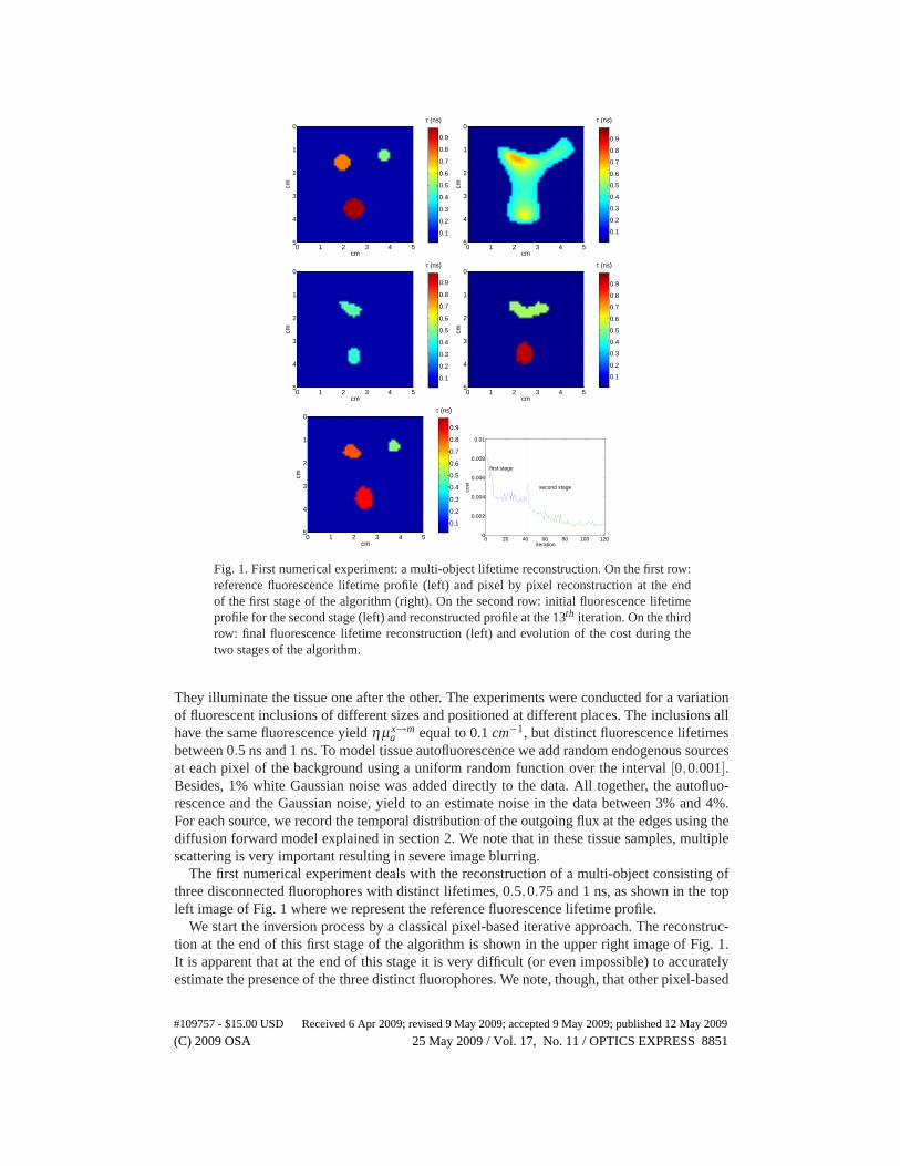
Fig. 1. First numerical experiment: a multi-object lifetime reconstruction. On the first row:reference fluorescence lifetime profile (left) and pixel by pixel reconstruction at the endof the first stage of the algorithm (right). On the second row: initial fluorescence lifetimeprofile for the second stage (left) and reconstructed profile at the 13th iteration. On the thirdrow: final fluorescence lifetime reconstruction (left) and evolution of the cost during thetwo stages of the algorithm.
They illuminate the tissue one after the other. The experiments were conducted for a variationof fluorescent inclusions of different sizes and positioned at different places. The inclusions allhave the same fluorescence yield ημx→m
a equal to 0.1 cm−1, but distinct fluorescence lifetimesbetween 0.5 ns and 1 ns. To model tissue autofluorescence we add random endogenous sourcesat each pixel of the background using a uniform random function over the interval [0,0.001].Besides, 1% white Gaussian noise was added directly to the data. All together, the autofluo-rescence and the Gaussian noise, yield to an estimate noise in the data between 3% and 4%.For each source, we record the temporal distribution of the outgoing flux at the edges using thediffusion forward model explained in section 2. We note that in these tissue samples, multiplescattering is very important resulting in severe image blurring.
The first numerical experiment deals with the reconstruction of a multi-object consisting ofthree disconnected fluorophores with distinct lifetimes, 0.5,0.75 and 1 ns, as shown in the topleft image of Fig. 1 where we represent the reference fluorescence lifetime profile.
We start the inversion process by a classical pixel-based iterative approach. The reconstruc-tion at the end of this first stage of the algorithm is shown in the upper right image of Fig. 1.It is apparent that at the end of this stage it is very difficult (or even impossible) to accuratelyestimate the presence of the three distinct fluorophores. We note, though, that other pixel-based
#109757 - $15.00 USD Received 6 Apr 2009; revised 9 May 2009; accepted 9 May 2009; published 12 May 2009
(C) 2009 OSA 25 May 2009 / Vol. 17, No. 11 / OPTICS EXPRESS 8851
cm
cm
0 1 2 3 4 5
0
1
2
3
4
5
τ (ns)
0.1
0.2
0.3
0.4
0.5
0.6
0.7
0.8
0.9
cm
cm
0 1 2 3 4 5
0
1
2
3
4
5
τ (ns)
0.1
0.2
0.3
0.4
0.5
0.6
0.7
0.8
0.9
cm
cm
0 1 2 3 4 5
0
1
2
3
4
5
τ (ns)
0.1
0.2
0.3
0.4
0.5
0.6
0.7
0.8
0.9
Fig. 2. Second numerical experiment: a T-shape fluorescence lifetime profile. Form left toright: reference fluorescence lifetime profile, final reconstruction at the end of the first stage(pixel by pixel reconstruction), and final fluorescence lifetime reconstruction at the end ofour algorithm.
schemes might be optimized (for instance, using more than the 4 sources in our experiments)yielding possibly slightly better results than those of our straightforward pixel-based imple-mentation. Nevertheless, the ’oversmoothing effect’ of regularized pixel-based schemes willstill apply making difficult to extract the important key characteristics of these images.
To continue with a shape-based approach we first replace the reconstructed pixel by pixelprofile achieved during the previous stage by the piecewise distribution shown in the centerleft image, as it was explained in Section 4. Once we have obtained this initial guess of theshapes of the fluorophores, we proceed with our shape-based reconstruction. The reconstructedfluorescence lifetime profile at the 13th iteration is shown in the center right image. Observe thatone object is breaking into two pieces. Each piece evolves during the next iterations changingits position, shape and fluorescence lifetime value. At the end of the process we obtain a verygood estimate of the key characteristics of the three different fluorophores, as it can be seen inthe bottom left image of Fig. 1.
It is interesting to compare the quality of our final reconstruction with the ’classical’ pixel-based reconstruction (using our own implementation) presented in the top right image. Theshape-based approach provides a much clearer identification of the different fluorophores anda more accurate estimation of their shapes and fluorescence lifetime values. This is so becausethe shape-based approach incorporates important prior information regarding the finite supportof the fluorophores, which cannot easily be incorporated in a classical pixel-based scheme.
In the bottom right image of Fig. 1 we show the evolution of the cost during the two stagesof the algorithm. At each stage, the cost is mainly monotonically decreasing until after a certainiteration becomes quasi-stationary.
In our second numerical experiment we want to recover a complex-shape fluorophore withτ = 0.75 ns, as shown in the left image of Fig. 2. As we can see, the reconstruction at the end ofthe first stage using the pixel-based approach, shown in the center image, gives rise to a roughestimate of the position of the fluorophore. However, because the diffusion of light results in theloss of imaging resolution we can not identify its shape. The shape-based algorithm applied tothe next iterations provides a much clearer identification of the fluorophore key characteristicssuch as its shape and fluorescence lifetime value, as shown in the right image.
Finally, we investigate a situation in which two small fluorophores are very close to eachother, as shown in the left image of Fig. 3. Their fluorescence lifetime is τ = 0.75 ns. Thecenter image shows the pixel by pixel reconstruction at the end of the first stage. The imageis too blurred and the two targets are not resolved. However, the shape-based reconstructionachieved at the end of our algorithm (see the right image) recovers the positions and shapes ofthe two fluorophores acurrately. The retrieved fluorescence lifetime value is also very good.
#109757 - $15.00 USD Received 6 Apr 2009; revised 9 May 2009; accepted 9 May 2009; published 12 May 2009
(C) 2009 OSA 25 May 2009 / Vol. 17, No. 11 / OPTICS EXPRESS 8852
cm
cm
0 1 2 3 4 5
0
1
2
3
4
5
τ (ns)
0.1
0.2
0.3
0.4
0.5
0.6
0.7
0.8
0.9
cm
cm
0 1 2 3 4 5
0
1
2
3
4
5
τ (ns)
0.1
0.2
0.3
0.4
0.5
0.6
0.7
0.8
0.9
cm
cm
0 1 2 3 4 5
0
1
2
3
4
5
τ (ns)
0.1
0.2
0.3
0.4
0.5
0.6
0.7
0.8
0.9
Fig. 3. Third numerical experiment: testing the spatial resolution. Form left to right: ref-erence fluorescence lifetime profile, final reconstruction at the end of the first stage (pixelby pixel reconstruction) and final fluorescence lifetime reconstruction at the end of thealgorithm .
6. Conclusions
We have presented a novel shape-based algorithm for fluorescence lifetime tomography. Tothis end, we have also derived the pixel-based gradients using an adjoint formulation. For theshape reconstruction problem we have employed level-set techniques that allow for an implicitrepresentation of the fluorophore shapes and frees us from topological restrictions during thereconstruction process. Our shape-based approach preserves the sharp edges of the fluorophoresthereby enhancing the contrast of the images. We believe that the results reported in this paperare important for the design of lifetime-based optical molecular imaging systems.
Appendix I
We derive here equations (15)-(18).To compute a descent direction of the cost (10) when μx→m
a varies, subject to conditions(1)-(2) and (5)-(6), we build the Lagrange function defined by
L (μx→ma ;Z,W ) = J (μx→m
a )−∫ T
0dt
∫Ω
drZ(r, t){1v
∂Ux(r, t)∂ t
−Dx∇2Ux(r, t)+(μxa + μx→m
a )Ux(r, t)−δ (r− rs)δ (t − t0)}︸ ︷︷ ︸A
−
∫ T
0dt
∫Ω
drW (r, t){1v
∂Um(r, t)∂ t
−Dm∇2Um(r, t)+ μma Um(r, t)−S(r, t)}
︸ ︷︷ ︸B
(23)
and we apply the adjoint method. Obviously, when Ux and Um satisfy Eqs. (1) and (2), A = B = 0and L = J for all Z and W , so we have incorporated conditions (1)-(2) into one function. Wenow take the derivative of Eq. (23)
δL =∂L
∂ μx→ma
δ μx→ma − ∂L
∂UxδUx − ∂L
∂UmδUm . (24)
Note that if the two last terms are zero then δL = δJ . Since, so far, Z and W are arbitrayfunctions, we can choose them so that these two last terms vanish, i.e., we impose that
∂L
∂UxδUx = 0 , (25)
∂L
∂UmδUm = 0 . (26)
#109757 - $15.00 USD Received 6 Apr 2009; revised 9 May 2009; accepted 9 May 2009; published 12 May 2009
(C) 2009 OSA 25 May 2009 / Vol. 17, No. 11 / OPTICS EXPRESS 8853
From these conditions we derive the adjoint equations.Let us now find the first ajoint equation. To first order we can write that
∂L
∂UxδUx = L (μx→m
a ,Ux +δUx,Um)−L (μx→ma ,Ux,Um) =
∫ T
0dt
∫Ω
drZ {1v
∂δUx
∂ t−Dx∇2δUx +(μx
a + μx→ma )δUx} . (27)
Integrating by parts, appying the divergence theorem, and using Eqs. (5) and (6) we obtain
∂L
∂UxδUx =
∫ T
0dt
∫Ω
drδUx {−1v
∂Z∂ t
−Dx∇2Z +(μxa + μx→m
a )Z} , (28)
where we have imposed that
Z(r, t = T ) = 0 in Ω and , Z(r, t) = 0 on ∂Ω . (29)
Since ∂L∂Ux
δUx have to be zero for all δUx, we arrive to an equation for Z. It reads
−1v
∂Z∂ t
−Dx∇2Z +(μxa + μx→m
a )Z = 0 . (30)
The minus sign in front of the time derivative in Eq. (30) means backwards time integration.The solution to this equation with ’initial’ and boundary conditions given by Eq. (29), vanishesin all the domain, i.e.,
Z(r, t) = 0 for all r ∈ Ω , and t ∈ [0,T ]. (31)
Similarly, to determine W we impose Eq. (26). To first order we obtain
∂L
∂UmδUm = L (μx→m
a ,Ux,Um +δUm)−L (μx→ma ,Ux,Um) =
∫ T
0dt
∫Ω
drW {1v
∂δUm
∂ t−Dm∇2δUm + μm
a δUm} , (32)
and
∂L
∂UmδUm =
∫ T
0dt
∫Ω
drδUm {−1v
∂W∂ t
−Dm∇2W + μma W} , (33)
where Eqs. (5) and (6) have been used, and where we have imposed that
W (r, t = T ) = 0 in Ω and , W (r, t) = R(μx→ma ) on ∂Ω . (34)
From Eq. (33) we get
−1v
∂W∂ t
−Dm∇2W + μma W = 0 , (35)
as we wanted.Therefore, if we select Z and W so that they satisty Eqs. (30) and (35), supplemented with
conditions (29) and (34), we have that
δJ = δL =∂L
∂ μx→ma
δ μx→ma =< gradμL , δ μx→m
a >P, (36)
#109757 - $15.00 USD Received 6 Apr 2009; revised 9 May 2009; accepted 9 May 2009; published 12 May 2009
(C) 2009 OSA 25 May 2009 / Vol. 17, No. 11 / OPTICS EXPRESS 8854
from where
δJ =< gradμJ , δ μx→ma >P =
∫Ω
dr∫ T
0dtW
∂S∂ μx→m
aδ μx→m
a , (37)
where < >P represents the inner product in the parameter space. To obtain Eq. (37), we havetaken the derivative of Eq. (23) with respect to μx→m
a and used the fact that Z vanishes in all thedomain. Note that Dx and S(r, t) depend on μx→m
a . Finally, taking the partial derivative of thesource S(r, t) with respect to μx→m
a in Eq. (37), we get that the gradient direction of J withrespect to μx→m
a is given by
gradμJ (r) =η
τ(r)
∫ T
0dtW (r, t)
∫ t
0dt ′e−(t−t ′)/τ(r)Ux(r, t ′) . (38)
With this we have proven equations (15)-(18).
Appendix II
In order to find a correction Δτ for the fluorescence lifetime distribution τ , we linearize the(nonlinear) residual operator (11), neglect terms of order O(||Δτ||2), and solve R[τ +Δτ] = 0.This amounts to solving
R ′[τ]Δτ = −R[τ] , (39)
where R ′ represents the derivative of R at τ . The minimum-norm solution of this equation canbe written as
Δτ = −R′[τ]∗ (R′[τ]R′[τ]∗)−1 R[τ], (40)
where R′[τ]∗ is the adjoint operator of R′[τ]. Since in our application the operator C =(R′[τ]R′[τ]∗)−1 is very expensive to calculate we approximate it by the identity operator I (notethat C acts as a ’filter’ from the parameter space to the parameter space). Using this approxima-tion, we just have to calculate
Δτ = −R′[τ]∗R[τ] . (41)
Note that R′[τ]∗R[τ] coincides with the gradient direction of J with respect to τ . Indeed,
J [τ +Δτ] = J [τ]+< gradτJ ,Δτ >P︸ ︷︷ ︸δJ
+O(||Δτ||2P) =
J [τ]+ < R′[τ]∗R[τ],Δτ >P +O(||Δτ||2P) . (42)
From Eq. (42), we can extract the gradient and write
gradτJ = R′[τ]∗R[τ] . (43)
Following the same steps as in Appendix I we readily find that
gradτJ (r) =∫ T
0dtW (r, t)
∂S∂τ
(r, t) , (44)
With this, and using Eqs. (43) and (41), we have proven Eq. (21).
#109757 - $15.00 USD Received 6 Apr 2009; revised 9 May 2009; accepted 9 May 2009; published 12 May 2009
(C) 2009 OSA 25 May 2009 / Vol. 17, No. 11 / OPTICS EXPRESS 8855