NASA/TP—2006-212490/VOL2/PART2 5–1

Flutter Prevention Handbook: A Preliminary Collection*

D.D. Liu, D. Sarhaddi, and F.M. Piolenc ZONA Technology, Inc.

9489 E. Ironwood Square Drive, Suite 100 Scottsdale, Arizona 85258–4578

Part D: Aeroservoelastic Instability, Case Study A

Raymond P. Peloubet, Jr.

Foreword

This report was prepared by ZONA Technology, Inc. under the support of the Flight Dynamics Directorate,

Wright Laboratory, USAF/AFMC/ASC, Wright-Patterson AFB, Ohio, 45433-7542, for the contractual period of January 1, 1995, through June 1, 1996, entitled “Flutter Prevention Handbook: A Preliminary Collection.” Mr. Ed Pendleton and Mr. Larry Huttsell of Wright Laboratory (WL/FIB) were the technical monitors under work units 2401TI00 and 2401LE00.

At ZONA Technology, the Principle Investigator was Dr. Danny D. Liu; Mr. Darius Sarhaddi and Mr. Marc de Piolenc were the editors.

We at ZONA Technology are grateful to the author for his willingness to contribute his lifelong knowledge in flutter technology, wherein the lessons learned throughout the history will be best appreciated by the dynamics engineers for many generations to come. It is hoped that the present report will be a first contribution to a future volumetric Flutter Prevention Handbook collection, complete in its entirety of world aircraft.

Equally, we are indebted to all the reviewers who spent their time and energy to this project in spite of other pressing demands. During the course of the contractual performance, the technical advice and assistance received from Larry Huttsell, Ed Pendleton, and Terry Harris of Wright Laboratory; Bob Moore of ASC/EN; Kenneth Griffin of Southwest Research; Thomas Noll of NASA Langley; Bill Reed of Dynamic Engineering Incorporated; and Victor Spain and Anthony Pototzky of Lockheed Engineering and Sciences Company are gratefully appreciated.

Finally, ZONA would like to acknowledge the USAF’s Aeronautical System Center’s History Office (ASC/HO) and the Air Force Museum research department (USAFM/MUA) for supplying many of the photographs used in this Handbook.

Abstract

The author presents two cases of aeroservoelastic instability, in which configurations that were flutter-stable

without their flight control systems becomes unstable at certain regimes with the control systems engaged. Part A discusses a high performance fighter with fly-by-wire control which showed antisymmetric oscillation in

early flight tests. Flutter analysis and wind tunnel tests showed the aircraft minus flight control system was stable. The Nyquist Criterion was used to calculate the stability of the airplane with the control system engaged; it showed an unstable antisymmetric oscillation mode very close in frequency to that observed in flight. Calculated control loop gain adjustments were tested in flight and found to correct the problem.

Part B concerns a fighter prototype with fly-by-wire control which showed a pitching motion in a narrow range of high-subsonic Mach numbers, at a frequency well below that of the first symmetric vibration mode of the *This document was taken from the original report: Liu, D.D.; Sarhaddi, D.; and Piolenc, F.M.: Flutter Prevention Handbook: A Preliminary Collection, WL–TR–96–3111, 1996, first published by the Flight Dynamics Directorate, Wright Laboratory, Air Force Materiel Command, Wright-Patterson Air Force Base.

NASA/TP—2006-212490/VOL2/PART2 5–2

structure and well above the rigid-body short-period mode. Subsequent flight tests showed that reducing the pitch loop gain eliminated the problem. Although the immediate problem was solved, two methods for measuring the open-loop frequency response function of the flight control system without actually opening the feedback loops were applied during flight tests. Both methods are explained and discussed.

Introduction

Flutter is an instability that is caused by the interaction of aerodynamic, elastic and inertia forces. The addition

of servomechanism forces as a fourth set of interactive forces can cause a flutter stable configuration to become unstable. This type of instability has been labeled as an aeroservoelastic (ASE) instability.

The servomechanism forces are usually generated by control surface deflections which are produced by hydraulic actuators controlled by servo valves. The input to the servo valves is the sum of the inputs from the pilot and the feedback from flight control sensors which have been passed through flight control laws. The control laws can be mechanized either by analog or by digital systems. However, other types of servo mechanism forces, such as vectored thrust systems, can produce ASE instabilities.

An appreciation for the cause of ASE instabilities can be obtained by considering a typical design process. First, flight control laws are designed to cause the airplane to respond in the desired manner to pilot inputs throughout the airplane's operational envelope. These control laws are usually developed with the airplane considered to be rigid. Initially, the only flexibility effect considered is the modification of the stability derivatives due to aeroelasticity. The flight control law designer might take several steps to reduce the likelihood of encountering an ASE instability.

• Sensors might be located to minimize their response to certain natural modes of vibration. For example,

vertical accelerometers might be located on the fuselage centerline close to a node line for the first fuselage bending mode. Similarly, pitch rate gyros might be located on the fuselage centerline near the maximum deflection on the first fuselage bending mode, where the slope would be zero and the pitch rate would be near zero.

• The flight control designer might select hydraulic actuators that have a low band pass. That is, the hydraulic

actuator produces one degree of control surface deflection for one degree of command to the actuator for frequencies from zero to some cut-off frequency (for example, 3 Hz). Above the cut-off frequency, the actuator produces lower deflection which continues to decrease as the frequency increases.

• The flight control law designer can incorporate low pass filters in the control law which diminish the

feedback signal for frequencies above some selected cut-off frequency, and/or notch filters which reduce the feedback signal in selected frequency bands.

However, in spite of these precautions, the response of one or more of the flight control sensors to the excitation

of a structural natural mode of vibration might produce a feedback signal of sufficient magnitude and with the right phase angle to cause an ASE instability.

Sometimes it is difficult to determine if an instability encountered in flight is caused by flutter or ASE. That is, if the unstable boundary is approached at constant altitude by slowly increasing airspeed from the stable side of the boundary, the instability might first appear as constant amplitude oscillations for either type of instability. It is important to distinguish which type of instability is involved because the type of correction needed is different. If the instability is caused by flutter the needed correction might be to modify the structure, or the mass distribution, or the aerodynamic configuration (by adding vortex generators or fences, for example). If, on the other hand, the instability is an ASE instability, the solution is usually to modify the flight control system or control law.

If the flight control system lowers the flutter boundary by a small increment, modifications to the flight control system might only restore that small increment. Further incremental increases to the flutter boundary might well require "flutter type" modifications. If the flight control system increases the flutter boundary by a small increment,

NASA/TP—2006-212490/VOL2/PART2 5–3

further increases in the boundary might best be achieved by flutter type modifications. Sometimes, however, a modification to the flight control system or the addition of a separate independent control system can increase the flutter boundary substantially or remove it entirely. In these cases the control system is called a flutter suppression system.

A direct means of determining whether an instability encountered in flight is caused by flutter or ASE is to disengage the flight control system. This is a viable option if the ASE instability is caused by an autopilot and the pilot can override the autopilot with the basic flight controls. If, on the other hand, the instability is caused by a closed-loop flight control system in which small forces applied by the pilot to the flight controls produce large control surface deflections if the feedback loop is opened, disengaging the flight control system is not a viable option. That is, with the loop open, the pilot would be in danger of over controlling and subsequently losing control of the airplane. Furthermore, aircraft that are statically unstable and rely on the flight control system for stabilization would be statically unstable if the feedback loop were opened.

Methods used to distinguish a flutter instability from an ASE instability include: (1) Comparing flutter analyses with ASE analyses, (2) Conducting flight tests with a gradual reduction in flight control system gains (subject to flight control

safety limitations) and (3) Measuring the open-loop frequency functions in flight (without actually opening the flight control loop) at a

sequence of flight conditions that approach the unstable boundary (this is discussed in Case Study A).

Case Study A Airplane Description This case study is about a prototype of a highly maneuverable fighter aircraft that made its initial flight tests

during the early part of the 1970 decade. One of the advanced technology concepts that it employed was the fly-by-wire flight control system. The connection between the cockpit controls and the servo valves for the hydraulic actuators for each control surface was electrical rather than mechanical. The conventional control systems at that time, transferred pilot-commanded deflections of the stick and rudder pedals via mechanical linkages to deflect the servo valves. The fly-by-wire system transformed pilot applied-stick and rudder forces into electrical signals which were sent to the servo valves by means of electrical lines. Pilot-applied stick forces produced deflections that were so small as to be virtually imperceptible, so the stick was called a force stick. The airplane was statically unstable over part of its operational envelope and the flight control system was used to stabilize the airplane.

The airplane with missiles mounted on the wing tip launchers is shown in figure 1. Control surfaces included flaperons on the wings, all-movable horizontal tail surfaces and a rudder. The locations of the servos that com-manded the control surface actuators are shown. Electrical signals from the pilot controller and rudder pedals and the air data computer were input to the flight control computer which implemented the flight control laws. Electrical signals from the flight control computer were sent to the servos which commanded the control surface actuators. The airplane response to the control surface movement was sensed by the flight control sensors and the outputs of those sensors were returned to the flight control computer to close the loop. The flight control system had three primary loops:

• The longitudinal loop commanded the horizontal tail surfaces to move symmetrically; airplane response

was sensed by the normal accelerometer, the pitch rate gyro and the angle of attack sensor. • The roll loop commanded antisymmetric deflections of the flaperons and of the horizontal tail surfaces in

the ratio of 1.0 degree flaperon to 0.25 degree horizontal tail; airplane response was sensed by the roll rate gyro.

• The yaw loop commanded the rudder and the airplane response was sensed by the roll rate gyro, the yaw rate gyro and the lateral accelerometer.

NASA/TP—2006-212490/VOL2/PART2 5–4

Pre-Flight-Test Analyses and Tests

Flutter analyses were conducted without the flight control system. Analyses were conducted over a range of

Mach numbers and altitudes. Several configurations of the airplane were analyzed, including configurations with and without wingtip missiles, for several fuel load conditions. These analyses indicated that the unaugmented (without the flight control system) airplane had at least a 20 percent flutter margin throughout its flight envelope.

Ground vibration tests were conducted with the airplane held by a soft suspension system. Hydraulic power was supplied to all control surface actuators but the feedback loops for all flight control system sensors were left open. With the tip missiles installed, the first two antisymmetric modes that were obtained by the ground vibration tests are shown in figure 2.

After the ground vibration tests, the finite element stiffness matrix of the airplane was modified to improve the correlation between computed and measured natural modes of vibration. Flutter analyses were repeated and they continued to show the unaugmented airplane to have at least a 20 percent flutter margin throughout its flight envelop.

A one-quarter scale flutter model of the airplane was tested on a cable system in the NASA Langley Transonic Dynamics Tunnel. The flight control system was not included in the model. The wind tunnel tests indicated that the unaugmented airplane with and without the tip missiles had at least a 20 percent flutter margin throughout its flight envelope.

Stability analyses of the airplane were conducted with the airplane considered to be a rigid body and with the flight control system engaged. Stability derivatives used in these analyses were modified to include the effects of static aeroelasticity. These analyses indicated that the augmented airplane was stable. Hence no aeroservo instabilities would be expected at any point in the flight envelope if the airplane were rigid.

Ground tests of the airplane were conducted with the airplane resting on its landing gear. An oscillatory input signal was applied to each set of control surfaces and the frequency of the input was varied over a broad range. Each control loop was opened, one at a time, and the open-loop frequency response function (FRF) (the ratio of feedback response to control surface input as a function of input frequency) was measured. Previous experience with this type of ground testing supported the belief at that time that if the magnitude of the measured frequency response function did not exceed 0.5 regardless of the phase angle, then the airplane would not experience any ASE instabilities in flight. These tests were conducted with the flight control system gains varied to simulate a large number of Mach-altitude flight conditions. These tests indicated that the airplane should be free of ASE instabilities throughout its flight envelope.

NASA/TP—2006-212490/VOL2/PART2 5–5

An ASE analysis was conducted at one high Mach number, low altitude flight condition that was thought to be the most critical point. The results of these analyses indicated that the aircraft would be free of ASE instabilities at this flight condition. Subsequent post flight test analyses indicated that this flight condition was beyond the back side of the unstable region as predicted by analysis.

Flight Tests

Initial flights of the airplane were made with the wing tip missiles. In this configuration an antisymmetric

oscillation at approximately 6.5 Hz was first experienced during flight number 8. The oscillation was experienced at the three flight conditions shown in figure 3. The airplane was being accelerated slowly at a constant altitude when the oscillation first began. The pilot climbed and reduced speed to get out of the unstable region. Then he climbed and increased Mach number until the instability was repeated. This operation was then repeated a third time.

The oscillation was again encountered during a sustained climb over a large altitude range on flight number 9, as shown in figure 3.

The instability was probed in a systematic manner on flight number 10. The airplane was flown at selected combinations of Mach number and altitude. These flight conditions were held constant while control surface pulses were applied. The roll pulse was the most effective in exciting the lowly damped response at 6.5 Hz as the unstable boundary was approached. But no excitation was required when the boundary was reached or exceeded. The unstable boundary at 20,000 feet was established. At 30,000 feet, however, the instability did not occur even for much higher Mach numbers.

NASA/TP—2006-212490/VOL2/PART2 5–6

A composite of the stability data that was obtained during the three flights is shown in the lower part of figure 3. A line was drawn through the unstable points that were thought to be near the boundary of the instability and which divided all known stable flight conditions from all known unstable flight conditions. Since the instability did not exist at higher altitudes, the unstable boundary was expected to have a top and perhaps a back side as indicated by the dashed line continuation of the unstable boundary line.

During the 6.5 Hz antisymmetric oscillations, the output of the accelerometers mounted on the wing tip launchers, the horizontal tail tips and the vertical tail tip were consistent in magnitude and phase angle with the 6.5 Hz, first antisymmetric mode of vibration measured during the ground vibration tests and shown in figure 2.

Initially there was some uncertainty about whether the oscillations were caused by flutter or ASE. However, after a series of ASE analyses were conducted at 0.9 Mach number and sea level that indicated that the roll loop was causing an ASE instability, additional flight tests were conducted with systematic gain reductions in both the roll and yaw channels. These tests indicated that the instability no longer existed when the roll loop gain was reduced by 50 percent. There was no appreciable difference in the results when the yaw loop gain was reduced.

Post-Flight Analyses

To conduct the ASE analyses, it is desirable to add the flight control system equations to the equations of

motion used to conduct flutter analyses. It is desirable because any change in stability can be attributed to the addition of the flight control equations and not be confused by the possibility that the change resulted from using a different method of analysis or a different modeling of the stiffness, mass or unsteady aerodynamics.

Unsteady aerodynamics are most conveniently expressed as a function of reduced frequency. Conventional V-g flutter analyses are conducted by constraining the equations of motion to harmonic motion, selecting a value of reduced frequency, computing the aerodynamic terms for the selected reduced frequency and then solving for the roots of the determinant of the equations of motion in the form of frequency and structural damping pairs. Using the selected reduced frequency, each frequency root can be used to compute a velocity associated with that root. The structural damping root can be plotted versus the velocity. By repeating this process for several selected reduced frequencies, each point on that curve can be interpreted to be the required structural damping to produce flutter at

NASA/TP—2006-212490/VOL2/PART2 5–7

the associated frequency. The point on the curve where the required structural damping agrees with the real structural damping is called the flutter point.

The flight control equations are usually expressed as a function of the Laplace variable. Hence, these equa- tions can also be expressed as a function of frequency by substituting iω for the Laplace variable s. For a selected velocity, frequency could be converted to reduced frequency so that the flight control equations could be expressed as a function of the reduced frequency to be compatible with the unsteady aerodynamics in the flutter equations. However, since velocity is an unknown variable in the flutter equations, only roots with velocity identical to the assumed velocity in the flight control equations would be valid solutions. Iterative methods would have to be applied in order to determine solutions that were compatible with the assumed value of velocity for the flight control equations.

A method for determining ASE stability characteristics was selected for the study airplane which employs the same equations of motion used in the flutter analysis. It requires selection of a velocity (Mach number, altitude and speed of sound) so the analyses can be conducted in the frequency domain. The flight control equations are com-bined with the flutter equations in the frequency domain. The stability of the closed loop system is determined by computing frequency response functions at selected flight conditions. The frequency response functions have a physical meaning and can be measured on the airplane.

The method of analysis is explained by referring to the block diagram of a closed loop single-input-single-output system shown in the upper left of figure 4. For the present application, consider an airplane with a flight control system consisting of only a roll loop and a single roll rate sensor. In the diagram, xi would be the pilot commanded roll input signal. The symbol G would represent the transfer function relating roll rate response, xo, to aileron deflection for the unaugmented airplane. The symbol H would represent the transfer function for the roll loop relating feedback response to the roll rate gyro input. The sensor response, xo, to the pilot input for the closed loop system, expressed as a function of the Laplace variable, is

GHG

xx

i

o+

=1

(1)

The stability of this closed-loop system can be assessed by determining whether the denominator (1 + GH) has

any zeros on the right hand side of the Laplace plane. If it has one or more zeros on the right-hand side, it is unstable. If it has no zeros on the right-hand side, it is stable. If a function of the Laplace variable is infinite at a value of the Laplace variable, it is said to have a pole at that value. Hence, if the function (1 + GH) has a zero at some value of s on the right hand side of the Laplace variable plane, then the function G/(1 + GH) has a pole at the same value of s.

The Nyquist criterion states that if a function of the Laplace variable is evaluated over a closed clockwise path that encloses the entire right hand side of the Laplace plane, the number of times (N) this function encloses the origin in the clockwise direction is equal to the difference between the number of zeros (Z) and the poles (P) on the right-hand side of the Laplace plane.

N = Z – P (2)

The evaluation path is illustrated on the lower left part of figure 4. The path extends from the origin up the

frequency axis to plus infinity. Then it follows a path that would be traced by a vector of infinite magnitude rotating from +90 degrees, to zero degrees, to –90 degrees. The path is then closed by following the frequency axis from minus infinity to zero. For this application the function (1 + GH) would be evaluated for values of the Laplace variable along this path and plotted as illustrated by the lower center part of figure 4. In practice the function (1+GH) would be plotted over a finite path along the frequency axis from zero to some selected positive upper frequency. The characteristics of the plot for higher frequencies and for the infinite magnitude part for the plot can usually be deduced. Also, since poles and zeros of the function (1 + GH) are either real or appear as complex conjugate pairs, the plot of the function (1 + GH) for negative frequencies is the mirror image of the plot for positive frequencies. The lower right part of figure 4 illustrates that the equivalent criteria is to determine the

NASA/TP—2006-212490/VOL2/PART2 5–8

number of clockwise enclosures of the minus one point by the function GH. And the upper right part of figure 4 illustrates that the physical interpretation of GH is the open-loop frequency response function relating the feedback to the pilot input. This is a measurable function.

By plotting the function GH, the number of enclosures of the minus one point can be determined. Hence, the number of zeros on the upper right quadrant of the Laplace plane can be computed

Z = N + P (3)

The number of poles in GH is equal to the sum of the number of poles in G and H. If the unaugmented airplane

is stable, G has no poles on the right-hand side of the Laplace plane. The number of poles on the right-hand side of H can be determined by inspecting the block diagram of the flight control system and usually there are none. So in practice, if the plot of GH shows no clockwise enclosures of the minus one point, the closed-loop system is stable. If the plot of GH shows one or more clockwise enclosures of the minus one point, the closed-loop system is unstable.

ASE stability was determined by computing the open-loop frequency response function over a frequency range from near zero to a selected upper frequency. The equations of motion employed rigid body side translation, roll and yaw and antisymmetric modes of vibration as generalized coordinates.

[ ]{ } { }δ−= δrsrs AqA (4)

where

( )

δδδ +=≠+=

=+⎥⎥⎦

⎤

⎢⎢⎣

⎡+⎟

⎠⎞

⎜⎝⎛

ωω

−=

rrr

rsrs

rsrsrr

rs

QMAsrQM

srQMigA

112

In order to put the equations in the form usually employed in flutter analyses, they have been divided by –ω2.

NASA/TP—2006-212490/VOL2/PART2 5–9

∫∫

∫

δδ Δφω

=

Δφω

=

dSpQ

dSpQ

rr

srrs

2

2

1

1

(5)

where S indicates the area of integration.

In equation (4) the structural damping in each mode can be assumed to be the same in every mode and treated as an unknown variable for the purpose of conducting flutter analyses. Setting the determinant of the left-hand side to zero and solving for the roots yields the variables that are plotted in the V-g type of flutter analysis.

Alternatively, the velocity, Mach number and altitude can be held constant and the determinant of the left-hand side of equation (4) can be computed as a function of frequency and plotted. The stability can be determined by the method of Landahl.

These analyses were conducted for the case study airplane at Mach 0.9 for several altitudes. The analyses indicated that the unaugmented airplane was stable.

A block diagram of the roll and yaw channels of the flight control system are shown on figure 5. The control system was an analog system. It had several gains that could be changed manually on the ground and it had gains that were computed as a function of the flight condition and changed automatically. The roll and yaw channels were essentially decoupled from the pitch channel. Two of the gains were varied as a function of the angle of attack and hence coupled with the pitch channel. However, these gains varied as a function of the steady angle of attack and provided virtually no dynamic coupling. The block labeled MGR is a manual gain in the roll channel; it was initially set at a value of 0.2. The block labeled M.G. is a manual gain in the aileron-rudder-interconnect; it was set a value of 1.0. The blocks labeled GARI and Gα/57.3 are variable gains that are a function of the angle-of-attack. The block labeled F8 is a gain that varied as a function of the flight condition. The gains that varied as a function of the flight condition are tabulated in figure 6.

NASA/TP—2006-212490/VOL2/PART2 5–10

The actuator was represented by a no-load, no-flow transfer function. The transfer function is different when the actuator is operating against a load and when high hydraulic flow rates are required. The no-load, no-flow transfer function was used because of its simplicity and because it was thought to be appropriate for predicting the onset of low amplitude ASE oscillations.

Similarly, the actuator stiffness was treated as a spring with constant stiffness. It was computed at a high frequency where the stiffness of the dynamic actuator approaches the stiffness of the hydraulic fluid. It appears in the equations of motion by way of the natural modes of vibration which were computed with a stiffness matrix in which each actuator spring was represented by a finite element.

The block diagram of the airplane with the yaw loop is shown in figure 6. Note that the sensor transfer functions have been added to the feedback loop. These transfer functions relate the sensor outputs to the airplane motion at the sensor locations. Note also that a minus one has been added so that the feedback signal subtracts from the pilot input. The flight control system block diagram in figure 5 shows the feedback signal adding to the pilot output. However, the negative sign is embedded in the feedback system or in the signs associated with control surface deflection.

The roll loop as used in the frequency response analyses is shown in figure 7. One degree of pilot commanded aileron produces one degree of aileron deflection plus 0.25 degrees of differential horizontal tail deflection.

NASA/TP—2006-212490/VOL2/PART2 5–11

Equation (4) was used to compute the response of the generalized coordinates to rudder excitation.

[ ] { }rrrsr

s AAqδ

−−=⎭⎬⎫

⎩⎨⎧

δ1 (6)

The frequency response function for each of the yaw loop sensors was computed as follows:

[ ]

[ ]

[ ]⎭⎬⎫

⎩⎨⎧

δφω=

δφ

⎭⎬⎫

⎩⎨⎧

δψω=

δψ

⎭⎬⎫

⎩⎨⎧

δω−=

δ

r

ss

r

r

ss

r

r

ss

r

y

qi

qi

qha 2

(7)

where hs is side deflection at the lateral accelerometer location, Ψs is yaw deflection at the yaw rate gyro location, ϕs is roll angle at the roll rate gyro location, for unit amount of generalized coordinates qs. The feedback at the point where the yaw loop is broken, shown in figure 6, can be expressed in the following

form by substituting iω for the Laplace variable s.

( ) ( ) ( ) ⎟⎟⎠

⎞⎜⎜⎝

⎛δφ

ω+⎟⎟⎠

⎞⎜⎜⎝

⎛δψ

ω+⎟⎟⎠

⎞⎜⎜⎝

⎛δ

ω=δ φψ

rrr

ya

r Yy TTa

TFeedback (8)

NASA/TP—2006-212490/VOL2/PART2 5–12

Substituting equation (7) into equation (8) yields the frequency response function relating the feedback in the yaw loop to rudder excitation with both the yaw and roll loops open. This function is plotted in polar form on the left side of figure 8 for Mach 0.9 sea level flight condition. The upper left part shows the function when only the three rigid body degrees of freedom (DOF) are used. This figure has two scales. All data plotted inside the unit circle have a scale from zero to unity. Outside the unit circle, the scale is from unity to 11.4. This figure shows no enclosures of the minus one point. It is concluded that if the yaw loop were closed, the rigid body representation of the airplane would have no ASE instabilities.

NASA/TP—2006-212490/VOL2/PART2 5–13

The figure in the lower left part of figure 8 shows the same frequency response data that was computed for a 9 DOF representation of the airplane. This representation has the same three rigid body DOF along with six natural modes of vibration DOF. The two antisymmetric modes of vibration shown in figure 2 are included in this analysis. This figure indicates that if the yaw loop were closed, the 9 DOF representation of the airplane would be stable. The stability margins of an airplane with a flight control system are usually expressed in terms of gain margin and phase margin. The gain margin requirement is usually 6 dB, which means that the overall gain in the open-loop FRF could be increased by a factor of 2 before the closed-loop system became unstable. This requirement is equivalent to the requirement that the maximum allowable magnitude of the open-loop FRF (with all other loops closed) where it crosses the negative real axis on a Nyquist plot, shall not exceed 0.5. The magnitude of the maximum negative axis crossing is tabulated in figure 8 along with the frequency at which the crossing occurs. The phase margin is defined as the angle between the negative real axis and the phase angle of the open-loop FRF where it crosses the unit circle. The phase margin requirement for a flight control system is usually ±60°. This means that the open-loop FRF phase angle (with all other loops closed) could be increased or decreased 60° before the closed-loop system became unstable. The phase margins can be estimated from the plots on figure 8.

The next step in the analysis is to close the yaw loop. The numerator of the left hand side of equation (8) is the rudder signal that was fed back and the denominator was the rudder signal that was input. Hence, the rudder signal that is fed back due to the sensor input, including the sign change at the summer, can be expressed as follows.

( ) ( ) ( )φω−ψω−ω−=δ φψ Y

TTaT yyar (9)

Expressing the lateral acceleration, yaw rate and roll rate in terms of the generalized coordinates, as indicated

by equation (7) yields the following expression.

[ ]{ } ⎣ ⎦{ } ⎣ ⎦{ }

[ ]{ }s

ssssssar

qT

qiTqiTqhT

r

Yy

δ

φψ

=

ωφ−ωψ−ω−−=δ 2 (10)

Substituting equation (10) into (6) yields the equations of motion for the airplane with the yaw loop closed.

[ ]{ } { }[ ]{ } [ ]{ }ssrsrs qAqTAqA rrr δδδ −=−= (11) [ ]{ } 0=+ δ srs qAA r (12) The Nyquist plots shown on the left side of figure 8 indicate that the airplane with the yaw loop closed would be

stable at the Mach 0.9, sea level flight condition. Therefore, the closed loop system indicated by equation (12) is stable.

The equations of motion for the airplane with the yaw loop closed and excited by an oscillatory aileron command are as follows.

[ ]{ } { } arsrs ar AqAA δ−=+ δδ (13)

where δa means aileron plus horizontal tail differential deflection in the ratio of one degree aileron to 0.25 degrees horizontal tail.

The generalized coordinate response per δa can be computed from equation (13) and used to compute the roll rate at the sensor location per δa.

NASA/TP—2006-212490/VOL2/PART2 5–14

[ ]⎭⎬⎫

⎩⎨⎧

δφω=

δφ

a

ss

a

qi (14)

Using figure 7, the ratio of aileron feedback, at the point where the loop is open, to the aileron command can be

expressed as

( )aa R

TFeedbackδφ

ω=δ φ (15)

Substituting equation (14) into equation (15) yields the expression for the open loop feedback in the roll loop

with the yaw loop closed. This frequency response function was computed and is shown plotted in polar form on the right side of figure 8.

The plot in the upper right-hand side of figure 8 is for the airplane represented with 3 DOF. This plot shows no clockwise enclosures of the minus one point. This plot indicates that the rigid airplane with both the yaw and roll loops closed would be stable.

The plot in the lower right-hand side of figure 8 is for the airplane represented with 9 DOF. This plot shows one clockwise enclosure of the minus one point. The negative axis crossing has a magnitude of 1.15 at a frequency of 6.3 Hz. The direction of increasing frequency is shown by arrow heads on each of the plots of figure 8. The plot in the lower right-hand side of figure 8 indicates that the 9 DOF representation of the airplane is unstable when both the yaw and roll loops are closed and that the frequency of the instability is near 6.3 Hz. This frequency is very close to the frequency of the instability that was observed during flight tests. The large loop on the plot with its maximum magnitude centered near a phase angle of –135 degrees, is associated with the response of mode one in figure 2. This antisymmetric mode has a large component of fuselage roll to balance the large inertia roll moment produced by the wing and tip missile motion.

Additional information can be obtained from the plot in the lower right-hand side of figure 8. Since the negative axis crossing has a magnitude of 1.15, a gain reduction in the roll channel of 1/1.15 would cause the open-loop frequency response to pass through the minus one point. Hence, neutral stability would occur for this reduced gain at this flight condition. That gain and any higher gain would cause the instability to occur. To reduce the gain so that the magnitude of the negative axis crossing was 0.5 (6 dB gain margin), the gain in the roll loop would have to be reduced by a factor of 0.5/1.15 or 44 percent.

The analysis was repeated with the control loops closed in the reverse order. The same conclusions with respect to ASE instability should be obtained. Only additional gain and phase information should be obtained. Plots of the open-loop frequency response function with the roll loop closed first are shown on figure 9. Referring to the lower left-hand side plot (9 DOF), it can be seen that the open-loop frequency response for the roll loop with both loops open shows a clockwise enclosure of the minus one point. The magnitude of the negative axis crossing is 1.06 and the frequency is 6.3 Hz. This plot indicates that closing the roll loop with the yaw loop open would still cause the ASE instability.

The plot on the lower right-hand side of figure 9 is the open-loop frequency response for the yaw loop with the roll loop closed. Since the left-hand plot shows the system to be unstable with the roll loop closed, the forward loop, G, (airplane with the roll loop closed) has one pole on the right-hand side of the Laplace plane. Substituting P equal one into the right-hand side of equation (3), it can be seen that N has to equal minus one in order for the number of zeros on the right hand side of the Laplace plane to be zero. That is the plot of the open-loop frequency response function for the yaw loop, with the roll loop closed, would have to produce one counterclockwise enclosure of the minus one point in order to conclude that the airplane with both loops closed was ASE stable. If it did not produce one counterclockwise enclosure of the minus one point, the airplane with both loops closed would be unstable.

NASA/TP—2006-212490/VOL2/PART2 5–15

Returning to figure 9, the plot in the lower right hand side does show a counterclockwise loop but it does not enclose the minus one point. The counterclockwise loop has its maximum magnitude centered near a phase angle of approximately 100 degrees. Since a reduction in the yaw loop gain would reduce the magnitude of each point along radial lines from the origin, it can be seen that no amount of reduction of the gain in the yaw loop would cause the counterclockwise loop to enclose the minus one point. This plot confirms the conclusion that this airplane could be stabilized by reducing the gain in the roll loop but it could not be stabilized by reducing only the gain in the yaw loop. This conclusion was consistent with flight test results.

The two plots on the upper part of figure 9 show that the 3 DOF rigid body representation is stable with both loops closed. Therefore, regardless of the order in which the roll and yaw loops are closed the 3 DOF rigid representation indicates that the rigid airplane with both loops closed is stable and the 9 DOF representation indicates that the flexible airplane with both loops closed is unstable.

NASA/TP—2006-212490/VOL2/PART2 5–16

Although the analysis predicted the ASE instability which occurred during flight tests, the analysis did not predict as large a region of instability as was determined by flight tests. ASE analyses were conducted at Mach 0.9 at three altitudes, namely, sea level, 5,000 feet and 20,000 feet. Hence, the analysis indicated that the top of the unstable region was near 5,000 feet and the flight test data indicated that the top of the unstable region was at least as high as 20,000 feet.

Part of the unconservative characteristic of the analysis is attributed to the manner in which the computed aerodynamic terms for the rigid body DOF and the control surface aerodynamics were modified to agree with wind tunnel measured rigid stability derivatives corrected for aeroelastic effects. These stability derivatives were called flexible stability derivatives. The unsteady aerodynamic terms that were computed for the 3 DOF rigid body equations of motion were modified to agree with the flexible stability derivatives near zero frequency. When the 9 DOF analyses were conducted, six generalized coordinates representing six natural modes of vibration were added to the 3 DOF rigid body representation. All of the unsteady aerodynamic terms associated with the three rigid body modes in the 9 DOF analysis were the same as they were in the 3 DOF analysis (that is, corrected to agree with the flexible stability derivatives). No change was made to the computed unsteady aerodynamic terms that were pro-duced by adding the six natural mode generalized coordinates. Hence, the six natural modes produced additional aeroelastic effects on the rigid body stability derivatives.

Later ASE analyses were conducted using the residual flexibility method. This method computes the residual flexibility that exists when a truncated set of natural modes are used in the equations of motion. The aeroelastic effects produced by the truncated set of natural modes plus the effect produced by the residual flexibility method provided the correct total aeroelastic effect. Hence, the computed unsteady aerodynamics for the rigid body DOF need only to be corrected to agree with wind tunnel based rigid stability derivatives.

A second method which approximated the residual flexibility method was also used. The aeroelastic effect contributed by the truncated set of natural modes was computed. This effect was subtracted from the total desired aeroelastic effect and the difference was applied to the rigid body stability derivatives. Hence, the sum of the modified rigid body aerodynamic terms plus the contribution produced by the truncated set of modes produced approximately the desired aeroelastic effect.

Later ASE analyses using these two methods for applying aeroelastic effects to the rigid body stability deriva-tives plus other refinements in the parameters used in the analyses improved the correlation between analysis and flight test data.

The ASE analysis conducted immediately after the ASE instability was encountered during flight tests provided assurance that the instability was an ASE instability, rather than flutter, and indicated that reducing the gain in the roll channel would restore stability. Although flight test experience indicated that a 50 percent reduction in the roll channel gain would stabilize the airplane, the selected correction consisted of reducing the roll channel gain to 60 percent of its original value and adding a notch filter to the roll channel. The notch filter was centered near 6.5 Hz and provided an additional gain reduction in a frequency band centered near 6.5 Hz.

Source of Additional Information For a more in-depth description of the flight test experience, as well as a more detailed description of the ASE

analyses that were conducted to improve the correlation between analysis and flight test results, the interested reader is directed to reference 1, from which most of the figures in the present work were taken. Subsequent ground testing that was conducted for the purpose of improving the ASE mathematical model is reported in reference 2.

The ASE instability for the Case Study A airplane was also reported in reference 3 at the 16th Structures, Structural Dynamics and Materials Conference. At the same meeting a similar ASE instability on a different airplane was reported in reference 4.

Recent ASE encounters through 1978, earlier close encounters, ASE analysis techniques, testing techniques, and design requirements are discussed in reference 5.

NASA/TP—2006-212490/VOL2/PART2 5–17

Aeroservoelastic Instability, Case Study B

Introduction Most ASE instabilities occur near the frequency of a structural natural mode of vibration. The frequency of the

ASE instability for the Case Study A airplane with wing tip missiles, was very close to the frequency of the first antisymmetric natural mode of vibration of the structure. At or near the frequency of a structural natural mode, a small amount of oscillatory control surface deflection can cause a large response in the natural mode and a large output from the flight control sensors. The flight control system designer is usually successful in designing the system so that it does not destabilize one of the airplanes rigid body natural frequencies.

However, the instability for the Case Study B airplane occurred at a frequency that was considerably below the lowest structural natural frequency and above the frequency of the rigid body short period mode. The frequency at which the instability occurred can be explained as the frequency at which the phase lag in the open-loop frequency response function (FRF) increased to 180° and the magnitude equaled or exceeded unity.

Case Study B complements Case Study A in that it demonstrates the use of one method of distinguishing a flutter instability from an ASE instability which was not applied in Case Study A. Specifically, Case Study B describes the measurement of the open loop FRF in flight.

Case Study B Airplane Description The Case Study B airplane was a fighter prototype with a cranked delta wing planform. The configuration is

shown in figure 10. It had two sets of wing trailing edge control surfaces. The outboard control surfaces were called ailerons. They

extended from an over-wing fairing that housed the aileron actuators to the wing tip missile launchers. The inboard surfaces, called elevons, could be actuated differentially as ailerons and symmetrically as elevators. The elevon actuators were located at the inboard end of each elevon in the fuselage. The airplane had a vertical tail with a full span trailing edge control surface called the rudder. The rudder actuator was located at the lower end of the rudder.

NASA/TP—2006-212490/VOL2/PART2 5–18

Flight control was provided by an analog fly-by-wire system. Pilot inputs to the controller and the rudder pedals were transmitted electrically to the actuator servo valves. The servo valves and the actuators were combined into units called integrated servo actuators (ISAs), allowing the hydraulic fluid flow path between servo valves and actuators to be considerably shortened.

The airplane also had two sets of wing leading edge flap surfaces; these were not used for flight control. The configuration carried missiles on wing tip launchers. Additional external stores were carried under the

wing. Fuel was carried in the fuselage and in the wings.

Pre-Flight-Test Analyses and Tests

Flutter analyses, without the flight control system, were conducted with and without the tip missiles, for a wide range of fuel conditions and for many underwing store configurations. These analyses indicated that the airplane had at least a 20 percent flutter margin throughout its flight envelope.

Flutter model tests of the complete configuration without the flight control system were conducted in the NASA Langley Transonic Dynamics Tunnel. These tests indicated that the airplane without the flight control system had at least a 20 percent flutter margin through the transonic and low supersonic regions (to the wind tunnel limits).

Flight simulation studies indicated the airplane, with the flight control system engaged, to be stable throughout its flight envelope. These studies were conducted with the airplane considered to be a rigid body. Stability deriva-tives were determined by wind tunnel tests conducted with rigid models. The wind tunnel based stability derivatives were modified to account for aeroelastic effects.

ASE analyses were conducted. These analyses indicated that no ASE instabilities should be expected through-out the flight envelope. The symmetric ASE analyses for the basic configuration without underwing external stores, indicated that the lowest gain and phase margins occurred in a frequency range between 2.5 and 3.0 Hz. This fre-uency range is below the first symmetric structural natural mode frequency which was 5.6 Hz, and considerably above the airplane's short period mode frequency.

Flight Tests During flight tests the pilot reported feeling a pitching motion of the airplane. It occurred in a narrow Mach

number range between 0.9 and 0.95. It was experienced at all altitudes up to 40,000 feet. The oscillations were either constant amplitude oscillations or lowly damped oscillations. The frequency of the oscillations ranged from 2.0 to 2.5 Hz.

Several flights were conducted in an effort to find an aerodynamic oscillatory excitation mechanism as an explanation for the pitch oscillations. After these flight tests proved to be unsuccessful in determining the source of the oscillations, a decision was made to measure the open loop FRF in the flight control pitch channel, in flight. However, while preparations were being made to make these measurements, a second decision was made to reduce the gain in the pitch channel by 25 percent. Subsequent flight tests showed that a 25 percent reduction in the pitch channel gain eliminated the pitch oscillations. At this point the need to measure the open loop FRF in flight was considerably reduced. However, the plan to make the measurements was continued in order to obtain better visibility for other potential corrective actions.

The objective of measuring the open loop FRF is to determine the stability of the closed loop system, as illustrated in figure 11. A block diagram of a single input, single output closed loop system is shown on the upper left part of this figure. For this application, G(s) represents the airplane transfer function and H(s) represents the flight control pitch channel transfer function. The ratio of the feedback signal, Xf (s), to the input signal, Xi (s), is shown in the equation in the upper part of figure 11.

NASA/TP—2006-212490/VOL2/PART2 5–19

The open-loop FRF can be measured by physically opening the feedback loop at the point at which it would

subtract from the input signal. By applying an oscillatory input signal and measuring the oscillatory feedback signal, the open loop FRF relating the feedback signal to the input signal can be obtained, as illustrated by the block diagram and equation in the lower left part of figure 11.

It is not feasible to physically open the loop during flight tests because of the associated risks of losing control of the airplane. However, the open-loop FRF can be measured without physically opening the loop. Two methods for measuring the open-loop FRF with the loop closed are illustrated by the block diagram and the equations in the lower right part of figure 11.

To obtain the open-loop FRF by the direct method, an oscillatory input signal is applied and the FRF for the ratio of the feedback signal to the error signal xe is measured. The error signal is the difference between the input signal and the feedback signal. This method is called the direct method because the open-loop FRF is measured directly and requires no subsequent algebraic operation.

To obtain the open-loop FRF by the indirect method, an oscillatory input signal is applied and the FRF for the ratio of the feedback signal to the input signal is measured. This closed-loop FRF is called T. By substituting frequency for the Laplace variable for the closed-loop transfer function equation at the top of figure 11 and substituting T for the left hand side of the equation, the equation can be solved for the product GH. This result is shown in the lower right part of figure 11 as T divided by 1 – T and is labeled the Indirect Method. This method is called the Indirect Method because the closed-loop FRF T is measured and the open-loop FRF is obtained as the algebraic ratio T/(1 – T).

Both the direct and indirect methods were used to measure the open loop FRF with the loop closed, in flight. A block diagram of the pitch channel is shown in figure 12. The airplane block shows that the input to the airplane is the combined symmetric deflections of the elevons and the ailerons. The outputs of the flight control sensors were fed back through the pitch channel to produce the feedback signal. The flight control sensors were the angle of attack sensor, α, the vertical accelerometer, An, and the pitch rate gyro, Θ. During the FRF measurements, the excitation signal was applied through the autopilot while the pilot supplied input to maintain straight and level flight conditions at constant altitude and constant Mach number. The input signal was measured as the sum of the

NASA/TP—2006-212490/VOL2/PART2 5–20

excitation signal and the pilot signal. The feedback signal was measured at the point before it was subtracted from the input signal to produce the error signal. The locations of the three signals that were measured are shown on the upper left part of the block diagram in figure 12 and labeled as xi, xe, and xf.

The blocks in figure 12 that are labeled with an alphanumeric symbol beginning with the letter F are gains; both fixed and variable. The blocks labeled notch, lead lag, lag and high pass, indicate transfer functions for notch filters, lead lag functions, lag functions, and high pass filters. The blocks labeled ISA are the transfer functions for the integrated servo actuators. The blocks labeled sensors are the transfer functions for the angle-of-attack sensor, the pitch rate gyro sensor and the normal accelerometer sensor. The numerical value of the gains and the transfer functions are not given because the purpose of Case Study B is to show the results of measuring FRFs in flight; not to compare computed and measured FRFs. All gains were constant over the Mach number range from 0.85 to 1.0. Also, there was no variation in the transfer function blocks.

The FRF could be measured by applying the excitation at a discrete frequency and measuring the desired ratios at the discrete frequency. By repeating the measurements at a sufficient number of points the open-loop FRF could be produced. A more efficient method of measuring the FRF is by the use of a harmonic analyzer that employs the Fast Fourier Transform (FFT) algorithm. The FFT algorithm computes the discrete Fourier transform of a sequence of measurements equally spaced in time in a very efficient manner (minimum number of mathematical operations) if the number of time measurements is equal to a power of two (for example, 512 or 1024). A harmonic analyzer of this type was used to process the flight test data. This harmonic analyzer could accept 1024 measurements at equal time intervals and compute the FRF for the ratio of the two signals at 512 positive frequency points in approxi-mately 0.03 second after the last of the two sets of data had been received. Hence, the FRF could be computed in virtually real time. Therefore, the excitation signal through the autopilot did not need to be a discrete frequency. Any type of input signal could be used and the harmonic analyzer could compute the FRF.

Two types of excitation are commonly used to measure FRFs. One is commonly called sine sweep excitation and the other is called random excitation. Sine sweep excitation applies an excitation signal at a discrete frequency and the frequency is slowly changed by sweeping from a selected minimum frequency to a selected maximum

NASA/TP—2006-212490/VOL2/PART2 5–21

frequency or vice versa. The random excitation method was selected for the Case Study B airplane. One reason for this selection is because the random excitation produces airplane motion that feels to the pilot as if he is flying in random turbulence. Hence, the ride comfort (or discomfort) and the degree of difficulty in maintaining straight and level flight appears to the pilot to be approximately the same from the beginning to the end of the applied excitation period. Whereas, during the sine sweep excitation the airplane response at the pilot station can vary to large degree as the frequency is slowly changed. Hence, the pilot feels like he is on a roller coaster ride with varying degrees of difficulty in maintaining straight and level flight throughout the frequency sweep.

The harmonic analyzer that was used, processed the data supplied to it in blocks called records. Each record consisted of 1024 measurements, for each of two signals, at equal time intervals. For this application the time intervals or sampling rate was set such that a record length was approximately 25 seconds. Hence the time interval was approximately 25/1024 or 0.0244 seconds. The FRF frequency increments were 1/25 or 0.04 Hz. Since 1024 data points are transformed into 512 positive frequency increments, the frequency range was from 0.04 Hz to (512)(0.04 Hz) or approximately 20 Hz. To improve the statistical accuracy the process was repeated for many records and the FRF data were averaged. To reduce the total time that the excitation was applied and to obtain better statistical accuracy, a new record was analyzed when 25 percent of new data had been added to the previous record and the oldest 25 percent of the previous record had been discarded. Using this 75 percent overlap on successive records, 32 records could be processed and averaged in a total excitation time of 220 seconds. These data are tabulated in figure 13.

A comparison of the open-loop FRF as obtained by the direct and indirect methods for one flight condition is also shown on figure 13. The FRFs are plotted in polar form or as Nyquist plots. The dotted circle on each plot is the unit circle. Although the frequency range was normally from zero to 20 Hz, the data are plotted up to 8 Hz. The data are plotted for negative feedback systems so the minus one point is the critical point. To describe the direction of the plot with increasing frequency it is noted that the magnitude of the plot at the low frequency end is greater than the unit circle and as the frequency is increased the magnitude of the plot approaches the center of the unit circle. Hence, the direction of the plot with increasing frequency is clockwise. It can be seen that the two methods for obtaining the open-loop FRF, with the loop closed, produce results that are very nearly the same. In particular, both methods show a negative axis crossing with a magnitude of approximately 0.63, at a frequency near 2.25 Hz.

NASA/TP—2006-212490/VOL2/PART2 5–22

Since the measurements were made with the gain in the pitch channel reduced to 75 percent of the value that it had when the pitch oscillations were experienced, the magnitude of all points would be expected to be increased by the ratio of 1/0.75 or 4/3 if the measurements had been made before the gain reduction had taken place. Hence, the magnitude of the negative axis crossing would have increased from 0.63 to 0.84. This magnitude is very close to unity and would indicate that the closed-loop system would be stable but lowly damped.

The flight conditions at which the open-loop FRF was measured are shown in figure 14. Measurements were made at three Mach numbers for each of the three altitudes and at six Mach numbers for one altitude.

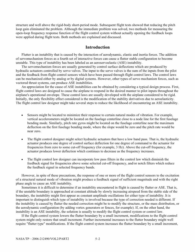
Plots of the open-loop FRF obtained by the direct method at 40,000 feet for each of six Mach numbers are shown on figure 15. It can be seen that the negative axis crossing has the largest magnitude at 0.95 Mach number and that the magnitudes at lower Mach numbers are progressively lower. The magnitude of the crossing at the higher Mach number is also significantly lower. Hence, these plots show that the closed-loop system would be the closest to unstable at 0.95 Mach number.

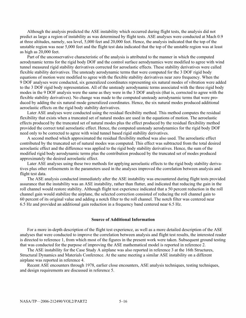
The magnitude of the negative axis crossings, or the crossings with 180 degree phase angle, are plotted versus Mach number at 40,000 feet on figure 16. The measurements were made with various levels of excitation input that are identified as low, intermediate and high levels. The measurements that were made with and without wing fuel are identified on the plot. The scale on the left indicates the magnitude of the crossings with the pitch channel gain reduced to 75 percent of its original value. The scale on the right has been increased by a factor of 4/3 to show the magnitude of the crossing that would have existed, by implication, before the gain was reduced. It can be seen that the implied negative axis crossing was very close to unity at 0.95 Mach number before the gain was reduced. Since the measured negative axis crossing does not equal or exceed unity for the 100 percent gain implies that meas-urement error accounted for the short fall or that the measurements were not made at the critical Mach number. That is, if the measurements had been made for smaller Mach number variations near 0.95 Mach number, a Mach number might have been found that produced a negative axis crossing that equaled or exceeded unity. However, the data that were obtained were in agreement with the original observations that the pitch oscillations occurred in a narrow Mach number range between 2.0 and 2.5 Hz.

The magnitude of the negative axis crossings at 20,000 feet and 10,000 feet versus Mach number are shown in figures 17 and 18. These plots indicate the minimum stability occurred at 0.92 Mach number at these two altitudes.

NASA/TP—2006-212490/VOL2/PART2 5–23

NASA/TP—2006-212490/VOL2/PART2 5–24

NASA/TP—2006-212490/VOL2/PART2 5–25

Summary The objective of measuring the open-loop FRF for the pitch channel, in flight, was to help diagnose the source

of the pitch oscillations experienced by the pilot during flight testing in a narrow Mach number range between 0.9 and 0.95, in a frequency range between 2.0 and 2.5 Hz. Before the open-loop FRF was measured, flight tests were conducted with the pitch channel gain reduced to 75 percent of its original value. The pitch oscillations no longer occurred after the gain was reduced. Hence, the need for measuring the open-loop FRF in flight was highly reduced. However, the planned measurement of the open-loop FRF in flight was continued with the pitch channel gain reduced to 75 percent of its original value.

By looking at figure 15 and visualizing what the sequence of open-loop FRFs would look like if the magnitude of each point was increased by a factor of 4/3, it can be seen that the measurements with the original pitch channel gain would have shown the minus one point to be very nearly enclosed by a clockwise enclosure. It would have been clear that the pitch oscillations were caused by the flight control system and that a reduction of the pitch channel gain would have stabilized the pitch oscillations. These plots would also have shown that the lowest gain margins occurred in the Mach number range between 0.90 and 0.95 and that the frequency ranged from 2.54 Hz at Mach 0.9 to 2.25 at Mach number 0.95.

It would also have been clear from the sequence of plots in figure 15 that the pitching oscillations were not likely to be caused by flutter. If flutter were the source of the instability, a clockwise loop near a structural mode frequency would have been expected at a low dynamic pressure flight condition, such as Mach number 0.7 at 40,000 feet. If flutter were the source of the pitch oscillations, the magnitude of the structural mode loop would have increased and the frequency at which the largest magnitude in the loop occurred would have approached the 2.0 to 2.5 Hz range as the flutter boundary was approached. Figure 15 does not show these characteristics. One can therefore conclude that flutter was not the likely source of the pitch oscillations.

The ASE analyses that were conducted prior to the flight tests showed open-loop FRFs that were similar to the ones shown in figure 15 in that the negative axis crossing with the largest magnitude occurred in the frequency range between 2.5 and 3.0 Hz. However, the magnitude of the negative axis crossing was not sufficiently high to expect an instability in flight. The ASE analyses might have under predicted the magnitude of the negative axis crossing because the reduction in the control surface effectiveness due to aeroelasticity in the transonic range, might have been over predicted. If the control surface effectiveness, in the transonic region, was predicted to be lower than it actually was, this under prediction would lead to the ASE analyses predicting lower negative axis crossings. It would also encourage the flight control system designer to increase the pitch channel gain to compensate for the reduction in the control surface effectiveness.

As the frequency increases from zero to approximately 2.25 Hz, the phase lag in the pitch channel open loop FRF increases to 180 degrees. The phase lag is produced primarily by the ISA and the pitch channel. The oscillations were not caused by a rigid body natural frequency, such as the short period mode, or by a natural structural mode. Instead, they occurred because the gain in the open loop FRF was too high when the phase angle was 180 degrees. The frequency of the oscillation was determined by the frequency at which the phase angle reached 180 degrees.

It was demonstrated during these flight tests that the open-loop FRF can be measured without actually opening the loop. Both the direct and indirect methods were used. For this application, the two methods yielded virtually the same open-loop FRF measurement.

Source of Additional Information The Case Study A airplane, without the tip missiles, encountered an instability in flight that was similar to

the instability encountered by the Case Study B airplane. With the tip missiles removed from the Case Study A airplane, the first antisymmetric natural mode of the structure is 8.0 Hz. The Case Study A airplane without the tip missiles encountered an instability at a frequency near 3.5 Hz. This frequency is far below the first natural

NASA/TP—2006-212490/VOL2/PART2 5–26

frequency of the structure and above the rigid body natural frequency. This instability is reported in references 1, 2 and 3.

Techniques for measuring the open-loop FRF without physically opening the loop were developed and demonstrated during wind tunnel tests of a flutter model with a flutter suppression system. These techniques and the results obtained by applying them are described in references 6, 7 and 8. To the author's knowledge, the first time these techniques were applied to an airplane in flight was when these techniques were applied to the Case Study B airplane.

Lessons Learned Some of the lessons learned from the experience gained from the Case Studies A and B are discussed. Conduct ASE analyses at multiple flight conditions.—It is generally not sufficient to conduct ASE analyses

only at maximum flight conditions. Flight control systems frequently employ variable gains that are scheduled to change as a function of flight conditions. Stability derivatives for a rigid airplane when plotted versus mach number frequently peak in the transonic region. Aeroelastic effects modify the stability derivatives for each flight condition. Hence, ASE analyses should be conducted for a sufficiently large number of flight conditions to ensure that the entire flight envelope has been adequately investigated.

Conduct ASE analyses for multiple external store configurations.—If the airplane carries external stores mounted on the wings, the natural modes of vibration can change with each store configuration. ASE instabilities can occur at different frequencies and at different flight conditions for different external store configurations. ASE analyses should be conducted for a sufficient number of store configurations to ensure that all possible external store configurations, including take-off store loadings and downloadings, have been adequately investigated.

Flight control system ground tests.—Open-loop FRF tests which are conducted on the airplane on the ground, should not be used, in lieu of ASE analyses, as a means of inferring ASE stability characteristics in flight. These tests are directly applicable only to the stability of the airplane on the ground. Open-loop FRF tests of the airplane on the ground (preferably supported by a soft suspension system to remove the effects of the landing gear) should be used to improve the correlation between the ASE mathematical model (without the aerodynamic representation) and the test data. One reason that ground tests are important is because flight control sensors are frequently located on the airplane where the response of the sensor is very low for one or more of the natural modes with the lowest frequencies. Hence, small errors in the computed mode shape at the sensor locations can make large percentage differences in the FRF.

Aeroelastic effects on stability derivatives.—The flight control system designer frequently conducts analyses with the airplane considered to be a rigid body. Stability derivatives are frequently obtained from wind tunnel tests of a rigid model. Hence these stability derivatives are sometimes called rigid stability derivatives. Aeroelastic effects are frequently computed by using a stiffness matrix representation of the airplane structure. The rigid stability derivatives modified by aeroelastic effects are sometimes called flexible stability derivatives. The flexible stability derivatives are used by the flight control designer.

When ASE analyses are conducted, the unsteady aerodynamic terms are computed. If only rigid body DOF are to be used in the analysis, the computed unsteady aerodynamic terms should be modified so that they agree with the flexible stability derivatives as the frequency approaches zero.

If both rigid body DOF and natural modes of vibration DOF are included in the ASE analysis, the modification of the rigid body unsteady aerodynamics varies with the number of natural modes included in the analysis. The same stiffness matrix that was used to conduct the static aeroelastic analysis should be used to compute the natural modes. If a lumped mass is located at each of the aerodynamic loading points used in the aeroelastic analysis, then the stiffness matrix is loaded with inertia loads in the vibration analysis at the same loading points used in the aeroelastic analysis. The maximum number of modes that can be computed is equal to the number of mass points. If all of the natural modes are included in the ASE analysis then the computed unsteady aerodynamic terms for the rigid body DOF should be modified to agree with the rigid stability derivatives as the frequency approaches zero. That is, the complete set of natural modes produces the same aeroelastic effect, as the frequency approaches zero, as the stiffness matrix produced in the aeroelastic analysis.

NASA/TP—2006-212490/VOL2/PART2 5–27

When a truncated set of modes (subset of the total number of modes) is used in the analysis (to reduce com-putational costs), only part of the stiffness effect is represented. If a truncated set of modes is used in the ASE analysis, the computed unsteady aerodynamic terms for the rigid body DOF should be modified, such that the sum of the aeroelastic effects in the modified rigid body aerodynamic terms plus the aeroelastic effect produced by the truncated set of modes, equals the correct total aeroelastic effect, as the frequency approaches zero. It should be noted that control surface aerodynamic terms are included when modifying computed unsteady aerodynamic terms for the rigid body DOF. Methods for making aerodynamic modifications are discussed in reference 1.

Measure open-loop FRF without physically opening the loop.—If an instability is encountered during flight tests the source of the instability is frequently in doubt. The measurement of the open-loop FRF at a series of speeds approaching the speed at which the instability was encountered, can be an effective means of determining whether the instability is primarily ASE or flutter. It is also useful in determining the changes needed to eliminate the instability.

References

1. Peloubet, R.P., Jr., et al.: Application of Three Aeroservoelastic Stability Analysis Techniques. AFFDL–TR–76–89, September 1976. 2. Peloubet, R.P., Jr., et al.: Ground Vibration Testing of Fighter Aircraft With Active Control Systems. AFFDL–TR–76–110, 1976. 3. Peloubet, R.P., Jr.: YF16 Active-Control-System/Structural Dynamics Interaction Instability. AIAA−1975−0823, 1975. 4. Arthurs, T.D.; and Gallagher, J.T.: Interaction Between Control Augmentation System and Airframe Dynamics on the YF−17.

AIAA−1975–0824, 1975. 5. Felt, Larry R., et al.: Aeroservoelastic Encounters. J. Aircraft, vol. 16, no. 7, 1979, pp. 477–483. 6. Peloubet, R.P., Jr.; Haller, R.L.; and Bolding, R.M.: F−16 Flutter Suppression System Investigation Feasibility Study and Wind Tunnel

Tests. J. Aircraft, vol. 19, no. 2, 1982, pp. 169−175. 7. Peloubet, R.P., Jr.; Haller, R.L.; and Bolding, R.M.: Wind Tunnel Demonstration of an Active Flutter Suppression System Using F−16

Model With Stores. AFWAL–TR–83–3046−VOL−2, 1984. 8. Peloubet, R.P., Jr.; Haller, R.L.; and Bolding, R.M.: Recent Developments in the F−16 Flutter Suppression With Active Control

Program. J. Aircraft, vol. 21, no. 9, 1984, pp. 716−721.