www.vacet.org E. Wes Bethel Lawrence Berkeley National Laboratory E. Wes Bethel Lawrence Berkeley National Laboratory Foghorns, Lighthouses and the Circuitous, Hazard-laden Path Towards Extreme Scale Data Analysis ICAP 2009 4 September 2009 San Francisco, CA Foghorns, Lighthouses and the Circuitous, Hazard-laden Path Towards Extreme Scale Data Analysis ICAP 2009 4 September 2009 San Francisco, CA
Transcript
www.vacet.org
E. Wes BethelLawrence Berkeley National Laboratory
E. Wes BethelLawrence Berkeley National Laboratory
Foghorns, Lighthouses and the Circuitous, Hazard-laden Path Towards
Extreme Scale Data Analysis
ICAP 20094 September 2009San Francisco, CA
Foghorns, Lighthouses and the Circuitous, Hazard-laden Path Towards
Extreme Scale Data Analysis
ICAP 20094 September 2009San Francisco, CA
Context
Rocks, Shoals, Wrecks, and Other Hazards• Data: size, complexity, I/O, formats, etc.
– It takes a long time to read, write big data.– Incompatible formats cause big problems.
• Working with big data: visual data analysis.– Can you run a 1TB file through gnuplot or IDL?– Does gnuplot or IDL really do what you need?
• Data: size, complexity, I/O, formats, etc.– It takes a long time to read, write big data.– Incompatible formats cause big problems.
• Working with big data: visual data analysis.– Can you run a 1TB file through gnuplot or IDL?– Does gnuplot or IDL really do what you need?
Remember When: 1981
This is no joke!
Data Problems
• Serial vs. parallel I/O.– One vs. many write streams.
• Formats:– How data is written out to disk: what order, storage
format, etc.– ASCII (ouch) vs. <many options>– Want: format compatibility along the tool chain.
• Serial vs. parallel I/O.– One vs. many write streams.
• Formats:– How data is written out to disk: what order, storage
format, etc.– ASCII (ouch) vs. <many options>– Want: format compatibility along the tool chain.
Format Propagation Issues
• What happens if each application in a tool chain uses its own unique data model/format?
• What if one or more formats changes during a weekend coding session?
• What if you want to look at results from a few years ago?
• What if you want to share results with your colleagues?
• What happens if each application in a tool chain uses its own unique data model/format?
• What if one or more formats changes during a weekend coding session?
• What if you want to look at results from a few years ago?
• What if you want to share results with your colleagues?
Data Format Solutions
– HDF, netCDF: partial solution (why partial?)• Data layout inside HDF5 file: your choice.• Data group naming inside HDF5 file: your choice.
– H5part: more complete solution.• What is H5part?
– Veneer API sits atop HDF5 (LBNL+PSI effort)– Simplifies use of HDF5.
• Opaque group naming.• Layout defined, managed by H5part.• Open Source, see vis.lbl.gov
Parallel I/O
• Achieving good I/O rates– How many streams?– Buffer sizes?
• Achieving good I/O rates– How many streams?– Buffer sizes?
Rocks, Shoals, Wrecks, and Other Hazards• Data: size, complexity, I/O, formats, etc.
– It takes a long time to read, write big data.– Incompatible formats cause big problems.
• Working with big data: visual data analysis.– Can you run a 1TB file through gnuplot or IDL?– Does gnuplot or IDL really do what you need?
• Data: size, complexity, I/O, formats, etc.– It takes a long time to read, write big data.– Incompatible formats cause big problems.
• Working with big data: visual data analysis.– Can you run a 1TB file through gnuplot or IDL?– Does gnuplot or IDL really do what you need?
Big Problem – Information Overload
• Our ability to create and store information exceeds our capacity to understand it.
• Information requires attention to process:– “A wealth of information creates a poverty of
attention.” – Hebert Simon, Nobel Prize, 1971.• Major challenge: gain insight from data.
– Visualization, visual data analysis are excellent tools for accomplishing this objective.
Query-Driven Visualization
• What is Query-Driven Visualization?– Find “interesting data” and limit visualization, analysis,
machine and cognitive processing to that subset.• One way to define “interesting” is with compound
boolean range queries.– E.g., (CH4 > 0.1) AND (T1 < temp < T2)
• Quickly locate those data that are “interesting.”• Pass results along to visualization and analysis
pipeline.• Another view: “remove the haystack to see needles.”
Query-Driven Visualization
Data Vis Render
The Canonical Visualization Pipeline
Query-Driven Visualization
Vis Render
Index
DataQuery
FastBit
(RegionGrowing)
DEX
Query-Driven Visualization
CH4 > 0.3
Temp < T1
CH4 > 0.3 AND temp < T1
CH4 > 0.3 AND temp < T2 T1 < T2
Query-Driven Visualization
• Compare performance to isocontouring.• For n data values and k cells intersecting the surface:
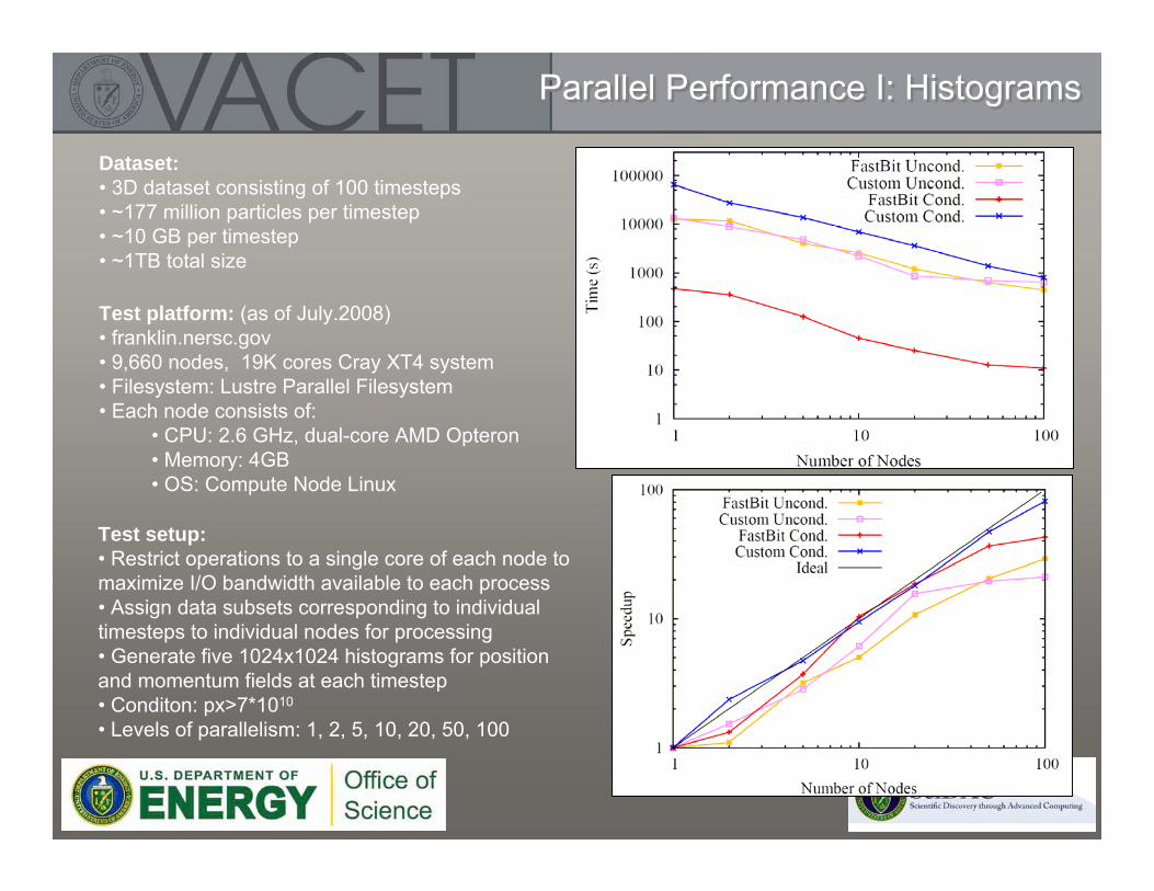
Test setup:• Restrict operations to a single core of each node to maximize I/O bandwidth available to each process• Assign data subsets corresponding to individual timesteps to individual nodes for processing• Generate five 1024x1024 histograms for position and momentum fields at each timestep• Conditon: px>7*1010
Test setup:• Same as for histogram computation• Track 500 particles (Condition: px>1011) over 100 timesteps
Results:• FastBit is able to track 500 particles over 1.5TB of data in 0.15 seconds
Performance of original IDL scripts:• ~2.5 hours to track 250 particles in small 5GB dataset
More Than Just a Research Project
• Several technologies from this project have been “productized” in VisIt and are available to “the entire world.”– Parallel coordinates interface (traditional and
histogram-based)– H5part, FastBit-enabled file loader to support
parallel collective I/O, including index/query.– ID-based, or “named” queries.
Concluding Remarks
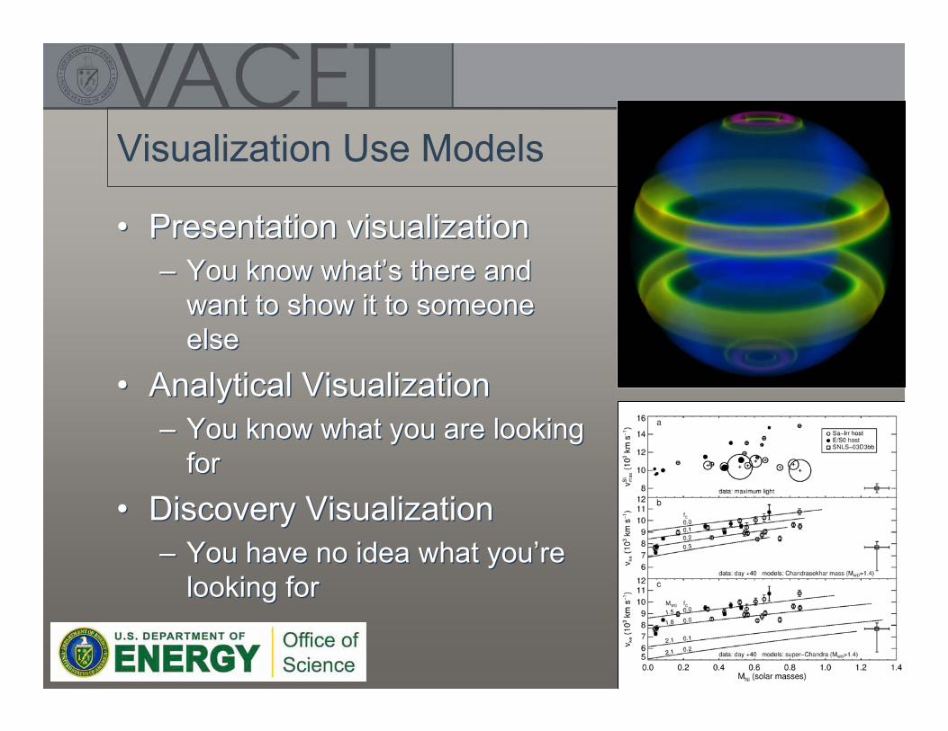
Visualization Use Models
• Presentation visualization– You know what’s there and
want to show it to someone else
• Analytical Visualization– You know what you are looking
for• Discovery Visualization
– You have no idea what you’re looking for
• Presentation visualization– You know what’s there and
want to show it to someone else
• Analytical Visualization– You know what you are looking
for• Discovery Visualization
– You have no idea what you’re looking for
Hazards at PScale and Beyond
• Computing hazards: out of scope for this talk.– E.g., solvers, multicore, 10M-100M cores, programming and
execution models, etc.
• I/O hazards:– Serial vs. parallel I/O– Data models and formats.
• Visual data analysis hazards– What problem are you trying to solve?– Sufficiently capable tools?– Effective tools?– I/O issues, data duplication?