Page 1
-~ -.--
(NASA-CR-139146) A GUIDANCE AND N75-1097NAVIGATION SYSTEH FOR CONTINUOUSLOB-THRUST VEHICLES M.S. Thesis(Bassachusetts Inst. of Tech.) 94 p HC Unclas$4o75 CSCL 17G G3/13 02592
TE 53
A GUODANCE AND NAVGATO~ SYSTEM -
FOR CONTINUOUS LOW THRUST VEH CL
CHARLES JACK - CHING TSE
SEPTEMB7R, o73
-KIKH'ati, KK-w ll
~14~P94v
https://ntrs.nasa.gov/search.jsp?R=19750002900 2018-09-05T15:41:44+00:00Z
Page 2
A GUIDANCE AND NAVIGATION SYSTEM
FOR CONTINUOUS LOW-THRUST VEHICLES
by
Charles Jack-Ching Tse
S. B., Massachusetts Institute of Technology
(1972)
SUBMITTED IN PARTIAL FULFILLMENT
OF THE REQUIREMENTS FOR THE
DEGREE OF MASTER OF SCIENCE
at the
MASSACHUSETTS INSTITUTE OF TECHNOLOGY
August, 1973
Signature of Author L J 4i 5 -..
Department of Aeronauticsand Astronautics, August, 1973
Certified by
Thesis Supervisor
Accepted by /- C ck l( -
Chairman, lDepartmental
Page 3
ERRATA SHEET
p. 10 n/ I should be n/u in the definition of n1,n2,n 3
x Wp.2 0 p x should read p" WP l+wz zwV
q = y should read q =z 2
p.40 numerators of the fractions in the first eqation shouldbe 3 instead of 1
Page 4
TE-53
A GUIDANCE AND NAVIGATION SYSTEM FOR
CONTINUOUS LOW THRUST VEHICLES
by
Charles Jack-Ching Tse
APPROVED:
DirectorMeasurement Systems Laboratory
Page 5
A GUIDANCE AND NAVIGATION SYSTEM FOR
CONTINUOUS LOW THRUST VEHICLES
by
Charles Jack-Ching Tse
Submitted to the Department of Aeronautics and Astronautics on.
August 29, 1973 in partial fulfillment of the requirements for the
degree of Master of Science.
ABSTRACT
A Midcourse guidance and navigation system for continuous low
thrust vehicles is developed in this research. The vehicle is requir-
ed to reach an allowable region near the desired geosynchronous orbit
from a near earth orbit in minimum time. The angular position of the
vehicle in the orbit is assumed to be unimportant during this midcourse
flight. The magnitude of the thrust acceleration is assumed to be
bounded. The effects of the uncertainties due to the random initial
state, the random thrusting error and the sensor error are included.
A set of orbit elements, known as the equinoctial elements, are
selected as the state variables. The uncertainties are modelled sta-
tistically by random vector and stochastic processes. The motion of
the vehicle and the measurements are described by nonlinear stochastic
differential and difference equations respectively.
A minimum time nominal trajectory is defined and the equation of
motion and the measurement equation are linearized about this nominal
trajectory. An exponential cost criterion is constructed and a linear
feedback guidance law is derived to control the thrusting direction
of the engine. Using this guidance law, the vehicle will fly in a
3 BLJDhING PAGE BLANK NOT man
Page 6
trajectory neighboring the nominal trajectory. The extended Kalman
filter is used for state estimation.
Finally a short mission using this system is simulated. The re-
sults indicated that this system is very efficient for short missions.
For longer missions some more accurate ground based measurements and
nominal trajectory updates must be included.
Thesis Supervisor: John Jacob Deyst, Jr., Sc.D.
Title: Associate Professor of Aeronautics and Astronautics, M.I.T.
4
Page 7
ACKNOWLEDGEMENTS
The author wishes to express his appreciation and graditude to
his thesis supervisor, Prof. John Deyst, Jr., who suggested the topic
of this thesis and provided close guidance throughout its development.
The author also owes a considerable debt of graditude to Mr. Theodore
Edelbaum and Dr. Robert Stern of the Charles Stark Draper Laboratory
for their helpful suggestions, their continued interest and support..
Acknowledgement is also made to the Charles Stark Draper Labora-
tory which provided the author with the use of its facilities.
This report was prepared under DSR Project 80539 sponsered by
the Goddard Spaceflight Center of the National Aeronautics and Space
Administration through Grant NGR 22-009-207.
5
Page 8
TABLE OF CONTENTS
Chapter Page
1 INTRODUCTION 15
2 THE MATHEMATICAL MODEL 17
2.A State Variables 17
2.B Equation of Motion 22
2.C Measurement Equation 24
2.D Statistical Modelling of the Uncertainties 26
2.E Statement of the Problem 29
3 THE GUIDANCE SYSTEM 31
3.A Nominal Trajectory 31
3.B Linearization 32
3.C Discretization 35
3.D Exponential Cost Criterion 37
3.E Solution of the LEG Terminal Cost Problem 40
3.F The Guidance System 44
4 THE NAVIGATION SYSTEM 47
4.A Extended Kalman Filter 47
4.B The Closed-loop Guidance and Navigation System 52
5 SIMULATION RESULTS AND DISCUSSION 55
5.A Simulation Results 55
5.B Discussion 72
6 CONCLUSIONS 75
-PRECEDING PAGE BLANK NOT F J 7
Page 9
Page
APPENDICES
A The Matrix x 79
B The Matrix . 81axC The Matrix 83- x
D The Matrix A (xu 0 ,t) 85
FIGURES
2.1 Equinoctial Coordinate Frame 19
2.2 Geometry of Earth-diameter and Star-elevation Measurements 25
2.3 Process Noise Vector 27
3.1 The Guidance System 45
4.1 The Navigation System 51
4.2 The Closed-loop System 53
5.1 (a) nominal vs t 56
5.2 (h)nominal vs t 57
5.3 (k)nominal vs t 58
5.4 (X0)nominal vs t 59
5.5 (P) nominal vs t 60
5.6 (q)nominal vs t 61
5.7 I(a)true - (a)nominall and I(a)true - (a)estimatedl vs t 66
5.8 I(h)true - (h) nominal and I(h)true - (h) estimatedl vs t 67
5.9 (k)true - (k) nominal and I(k)true - (k) estimated vs t 68
5.10 (10true (0 nominal and I(0 true (X)estimatedl vs t 69
5.11 I(P)true - (P)nominall and I(p)true - (P)estimatedl vs t 70
5.12 I(q)true- (q)nominall and I(q)true - (q)estimatedl vs t 71
REFERENCES 77
8
Page 10
LIST OF SYMBOLS
a Semi-major Axis
A - Gu
b x -
B G
d Diameter of Earth
e Eccentricity
e Eccentricity Vector
exp {.} Exponential
E {.) Expectation
f Unit Vector in the Equinoctical Coordinate Frame
F Eccentric Longtitude
90 Surface Gravity Acceleration
9 Unit Vector in the Equinoctial Coordinate Frame
G Matrix of partial derivatives of Equinoctial elements
with Respect to Velocity Vector
h Equinoctial element
h Measurement Vector Function
H - hDx
i Inclination
I Identity Matrix
Is Specific Impulse
I(6x ) Indicator Function for the Target Set
Im (t Indicator Function for the Control
JO Cost Criterion for the minimum Time Nominal
Trajectory
9
Page 11
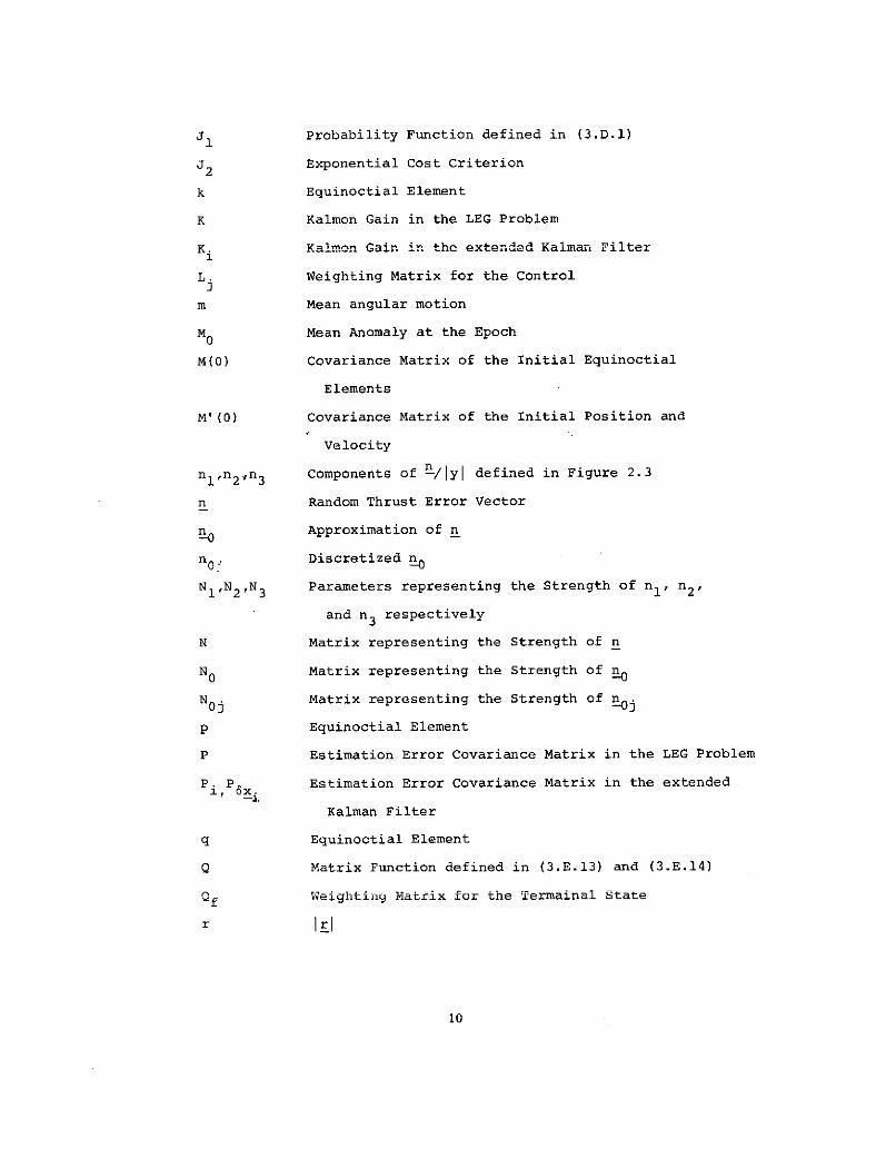
J1 Probability Function defined in (3.D.1)
J2 Exponential Cost Criterion
k Equinoctial Element
K Kalmon Gain in the LEG Problem
K. Kalmon Gain in the extended Kalman Filter
L. Weighting Matrix for the Control
m Mean angular motion
M0 Mean Anomaly at the Epoch
M(0) Covariance Matrix of the Initial Equinoctial
Elements
M'(0) Covariance Matrix of the Initial Position and
Velocity
n 1 ,n 2 n3 Components of n-/Iyl defined in Figure 2.3
n Random Thrust Error Vector
no Approximation of n
n0 Discretized n
NIN2N 3 Parameters representing the Strength of nl, n2,
and n 3 respectively
N Matrix representing the Strength of n
NO Matrix representing the Strength of n
NOj Matrix representing the Strength of 0j
p Equinoctial Element
P Estimation Error Covariance Matrix in the LEG Problem
PiP 6x Estimation Error Covariance Matrix in the extended-1
Kalman Filter
q Equinoctial Element
Q Matrix Function defined in (3.E.13) and (3.E.14)
Qf Weighting Matrix for the Termainal State
r |rl
10
Page 12
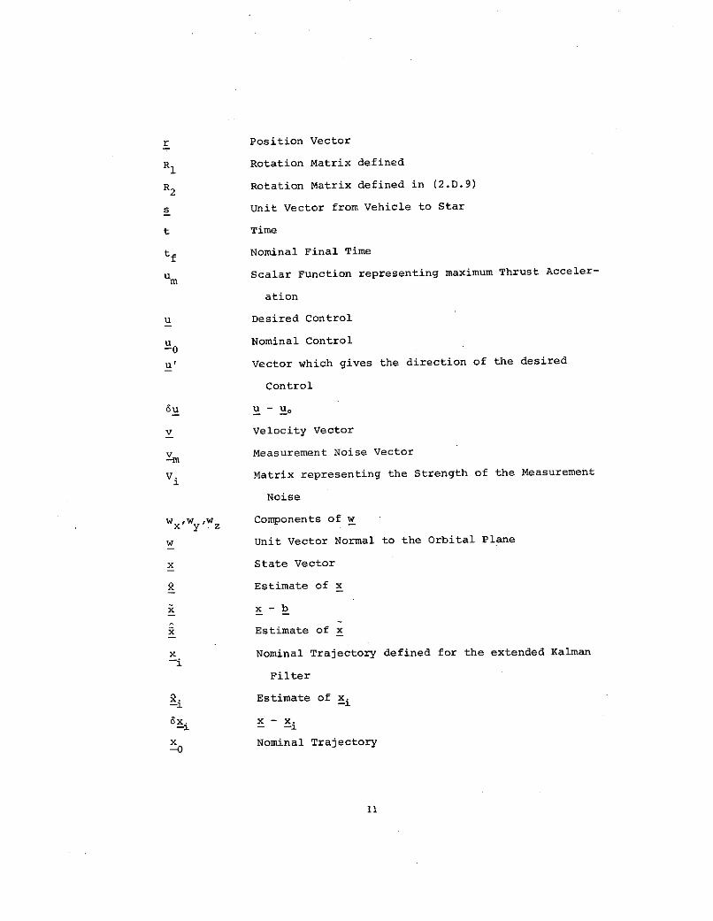
r Position Vector
R1 Rotation Matrix defined
R2 Rotation Matrix defined in (2.D.9)
s Unit Vector from Vehicle to Star
t Time
tf Nominal Final Time
u Scalar Function representing maximum Thrust Acceler-
ation
u Desired Control
u Nominal Control-0
u' Vector which gives the direction of the desired
Control
6u u - uo
v Velocity Vector
v Measurement Noise Vector-m
V. Matrix representing the Strength of the Measurement
Noise
xw y ,W Components of w
w Unit Vector Normal to the Orbital Plane
x State Vector
SEstimate of x
xx - b
x Estimate of x
x Nominal Trajectory defined for the extended Kalman-i
Filter
x. Estimate of x.-- 1 -- 1
6x. x - x.-- i - -- 1
x Nominal Trajectory011
11
Page 13
x (0) Expectation of x(0)
6x x - x- - -o
xf Target set Parameter defined in (2.E.2)
6x Target set Parameter defined in (2.E.2)-f
X1 Position Coordinate relative to the Orbital Frame
X1 Velocity Coordinate relative to the Orbital Frame
Xtarget Target Set
Y- Measurement Residual
Y Covariance Matrix of the Measurement Residual
1 Position Coordinate relative to the Orbital Frame
Y1 Velocity Coordinate relative to the Orbital Frame
z Measurement Vector
6z. Defined in (4.A.4)-- 1
a Angle defined in Figure 2.2
A Feedback Control Gain Matrix
8 Auxiliary Variable defined in (2.A.19)
y Constant defined in (3.E.4)
6(t-T) Dirac delta Function
6k. Kronecker delta
£ Initial Thrust Acceleration in terms of go's
A0 Equinoctial Element
SGraviational Constant
(ar 1 Standard Deviation of Position in Altitude Direction
(r )2 Standard Deviation of Position in Down Rang Direction
12
Page 14
(ar) 3 Standard Deviation of Position in Cross Track Direc-
tion
(oyv)l Standard Diviation of Velocity in Altitude Direction
(cy) 2 Standard Deviation of Velocity in Down Range Direc-
tion
(Gv)3 Standard Diviation of Velocity in Cross Track Direc-
tion
T Time
State Transition Matrix
Matrix Defined in (3,C,21)
w Arguement of Perigee
Longtitude of the Ascending Node
13
Page 15
CHAPTER I
INTRODUCTION
Recently, solar electric spacecraft propulsion systems of high
efficiency have been developed. The advancements of this new tech-
nology have opened the road to a new era of space exploration and
scientific research. Many space missions utilizing this propulsion
system have been planned by the National Aeronautics and Space
Administration for the second half of this decade. One of these
missions utilizes the solar electric propulsion stage (SEPS) for the
delivery and return of scientific payloads between near earth orbits
and the geosynchronous orbits-.
The purpose of this research is to develop a practical and
efficient midcourse guidance and navigation system for these continuous
low thrust vehicles. The vehicle is required to reach an allowable
region near the desired geosynchronous orbit in a minimum amount of
time. During this midcourse phase the angular position of the vehicle
in the orbit is assumed to be unimportant. The magnitude of the thrust
acceleration of the SEPS is constrainted to be bounded. The uncer-
tainties due to the random initial state, the random thrusting error
and sensor error are included..
In Chapter II a set of state variables is selected and a
mathematical model is constructed. The motion of the vehicle is
described by a nonlinear stochastic differential equation and uncer-
tainties are modelled by stochastic processes. In Chapter III a
minimum time nominal trajectory is defined and the equation of motion
pRECEDING PAGE BLANK NOT FMM15
Page 16
and measurement equation are linearized about this nominal trajectory.
A meaningful cost criterion is constructed and a linear feedback con-
trol law is derived for the guidance system. In Chapter IV a naviga-
tion system is constructed and the complete closed-loop system is
discussed. The computer simulation results of this system are
presented and discussed in Chapter V. Finally conclusions are
presented in Chapter VI and the various equations related to the state
variables are presented in the Appendix.
16
Page 17
CHAPTER II
THE MATHEMATICAL MODEL
The construction of a mathematical model is the most important
step in the design of a gudiance and navigation system for continuous
low thrust vehicles. In this chapter an appropriate set of state
variables is selected. Then the equations describing the motion of
the vehicle and the dynamics of the sensors are chosen. The uncertain-
ties due to the random initial state, the random thrusting error and
the sensor error are modelled statistically. Finally the problem
considered in this research is stated mathematically.
2.A State Variables
The state variables used in this research are the equinoctial
elements [4]. The most important advantage of these elements is
that their equation of motion are free from singularities for zero
eccentricity and zero inclination. This is not the case for the
classical orbit elements [2].
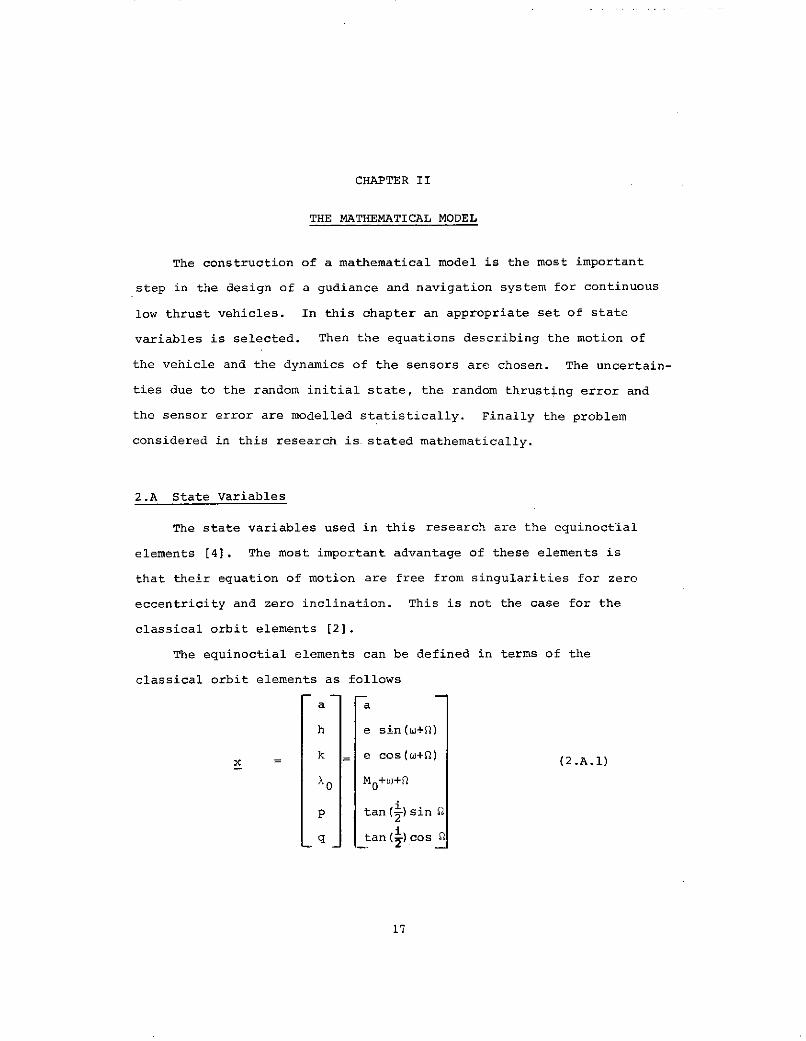
The equinoctial elements can be defined in terms of the
classical orbit elements as follows
a a
h e sin(w+Q)
k - e cos(w+Q) (2.A.1)
10 M0 +o+Q
p tan( )sin 0
q tan()cos "
17
Page 18
where a, e, i, Mo, w and 0 are the classical orbit elements
a = semimajor axis
e = eccentricity
i = inclination
M0= mean anomaly at the epoch
w = argument of perigee
0 = longtitude of the ascending node
Alternatively, the equinoctial elements can be defined in.terms
of the postition and velocity vectors. A coordinate system is defined
for this purpose as shown in Figure 2.1. The unit vector normal to
the orbital plane is given by
rxv
W x (2.A.2)
where r and v are the position and velocity vectors respectively.
The components of this vector can be written in terms of the classical
orbit elements as
w= R [0 0 1]T
sin 0 sin i
= -n cos n sin i (2.A.3)
L cos i jwhere R1 is the rotation matrix
cos 0 sinQ 0 1 0 0 cos 0 sin Q 0
R1= sin Q cos Q 0 0 cos i sin i -sin cos 0 (2.A.4)
0 0 1 0 sin i cosi 0 0 1
18
Page 19
z
f unit sphere
x
Equinoctial Coordinate Frame
Figure 2.1
19
41ivO
Page 20
Using (2.A.3) in (2.A.1) the equinoctial elements p and q can be
written in terms of these components
x (2.A.5)
S+ (2.A.6)
The unit vectors f and q defined in Figure 2.1 can now be written
in terms of p and q
Tf = R1 [1 0 0]
2 (A2 2
1 - p2 + q2
1 + p2 + q2 2 p q
L-2 p
_=R 1 [ 0 1 0]T
2 2 1 + p - q (2.A.8)
2 q
The elements h and k are seen to be the components of the eccentricity
vector in the directions of these unit vectors and are given by
h = e T g (2.A.9)
k = eT f (2.A.10)
where e is the eccentricity vector
r (rx v) xve - - (2.A.11)
20
Page 21
The element a is given by
a = 2 I - (2.A.12)Irl
If the components of the position and velocity vectors along the unit
vecotrs f and g are denoted by
x I = r f (2.A.13)
Ty = r g (2.A.14)
x= T f (2.A.15)X1 =
= v £(2.A.16)
the eccentric longtitude F can be written as
(1-k28)X 1 - h k BY1 (2.A.17)cos F = k +I (2.A.17)
a/l-h2 -k 2
(1-h2 )Y 1 - h k BX 1
sin F = h + (2.A.18)
where= 1 (2.A.19)
1 + /l-h 2-k 2
The remaining element X0 is given by Kepler's equation
0 = F - k sin F + hcos F- -- t (2.A.20)a
where t is the time measured from the epoch.
21
Page 22
These equations are the transformations from classical orbit
elements or position and velocity vectors to equinoctial elements.
The inverse transformation from equinoctial elements to position
and velocity is also included here for convenience.
To calculate the position and velocity vectors from equinoctial
elements, Kepler's equation (2.A.20) must be solved for the eccentri-
city longtitude F. Then the position and velocity vectors are given
by
r = X f + Y1 9
v = x f + Y1
Xl = al-h2 8)cosF+ h k 8 sinF - k] (2.A.23),
Y1 = a[l-k28)sinF + h k 8 cosF - h] (2.A.24)
-= [h k 8 cosF - (1-h28) sinF] (2.A.25)1 r
S= [ ( 1-k 2 8)cos F - h k 8 sinF] (2.A.26)1 r
where
r = a[l-k cosF - h sinF] (2.A.27)
2.B Equation of Motion
The only forces assumed to be acting on the vehicle are the
inverse square gravitational attraction of earth, the desired engine
thrust and the random thrusting error. The motion of the vehicle is
described by a nonlinear stochastic differential equation [10].
d = G(x,t)u + G(x,t)n (2.B.1)dt
22
Page 23
where u is the desired engine thrust, n is the random thrusting error
and G(x,t) is a 6x3 matrix of the partial derivatives of the equi-
noctial elements with respect to the velocity vector. The G(x,t)
matrix is given byax
Glx,t) =- (2.B.2)
where
S2a 2 vT (2.B.3)
v *
ah _ -h2-k 2 X1 a 1 1 T-- h )f + (7k- h
k(qY1 - pX1) T+ . (2.B.4)
ma 2 1-h 2 k 2
8k = l-h -k2 X Xl Y1 1-v = [(e- + k m -)f+ + kB j_-)g
h(qY1 - pXl) T
ma 2 J 1-2-k 2 (2.B.5)
O 2 - 3 T l-h -k
v [r - v t] + p [(hav ma2 2 ap a
2X1 Y1 1 T+ k f+ (h-- + k a )q]T
(qY1-PX1) T+ wT (2.B.6)
ma 2 / 1 -h 2 -k 2
23
Page 24
2 2S= +p 2 Y1 T
(2.B.7)
2ma 2/1-h 2-k2
S= l+p +q X w (2.B.8)
2ma2Vl-h2-k 2
2.C Measurement Equation
Sensors are used to make measurements and update the vehicle's
estimate of it's state. These measurements which are corrupted by
random sensor errors are assumed to be made at discrete instants of
time. The types and the schedule of these measurements are assumed
to be fixed. The measurement equation is given by
z(t ) = h(x, ti ) + Ym(ti) (2.C.1)
0 = ti<t2<... <tm = tf
where z(ti ) is the measurement vector, h(x,t i ) is a vector function
of the state and v (ti) is the vector of the random sensor error.-m
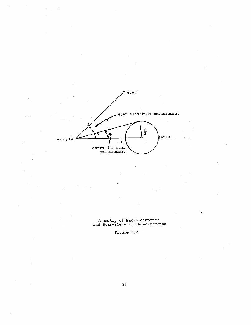
The form of the vector function h(x,ti)depends on the type of
measurement. For example, if a earth-diameter and a star-elevation
measurement are taken simultaneously, the vector function h(yxti)
given by
2 s i n - (2
h(x,t ) =cos
24
Page 25
star
star elevation measurement
arthvehicle
earth diametermeasurement
.Geometry of Earth-diameterand Star-elevation Measurements
Figure 2.2
25
Page 26
where s is the unit vector from the vehicle to the star and d
is the diameter of earth. These measurements are pictured in
Figure 2.2.
2.D Statistical Modelling of the Uncertainties
There are three sources of uncertainties considered. They are
the random initial state, the random thrusting error and the sensor
error. The initial state x(O) is assumed to be a Gaussian random
vector. The mean and covariance of this vector is denoted by
E[x(0)] = x (2.D.2)
E{[x(0) - x(0)][x(0)-x(0)] T= M(0) (2.D.2)
If the covariance matrix of the initial state is given in terms
of the position and velocity vectors, the necessary transformation
to the equinoctial elements is given by
M(0) = M'(O) _ I
(O) x (0)
where M'(0) is the covariance matrix of the initial position and
velocity vectors. The matrix ax/ar is included in the Appendix.
The random thrusting error is modelled by a zero mean white
Gaussian random process
E[n(t) ]=0 (2.D.4)
E[n(t)nT(T)] = N 6(t-T) (2.D.5)
The matrix N, representing the strength of the process noise, is
dependent on the desired engine thrust u. Both the n and u vectors are
pictured in Figure 2.3. The z' axis is defined in the direction
of the vector u. The x' and y' axes are defined in a plane normal
to u to form a triad. The quantities n,, n 2 and n 3 are assumed to
be zero mean independent random processes
26
Page 27
n 31 u
y'
Process Noise Vector
Figure 2.3
27
Page 28
E[n (t)] = 0 i=1,2,3 (2.D.6)
E[n.(t) n (T)] = N 6 (t-T) i=1,2,3 (2.D.7)
E[n(t) n(T)] = 0 i3ij (2.D.8)
These quantities are also assumed to be independent of the vector
u. Let R 2 be the orthogonal transformation such that
U R2[ 0 0 1] (2.D.9)
Then the vector n(t) and it's correlation can be written as
n = u R 2 [n 2 n n 3 ]T (2.D.10)
S n1 (t)n 1(T) nl(t)n 2 (T) n 1 (t)n3(T)
E[n(t)n T (T)] = E uI 2R2 2(t)n (T) n 2 (t)n2(T) n2(t)n 3 () RT
-2 1 22
S(t)nl () n 3 (t)n 2 (T) n3(t)n3 (T)
(2.D.11)
In view of (2.D.7) and (2.D.8), the correlation of n becomes
Nl 0 0E[n(t)n (T) = [u R2 R2 N2 0 R2 T 6(t-T) (2.D.12)
0 0 N3-
Furthermore since nl and n 2 are defined in a plane normal to u, it
is reasonable to assume that
N1 = N 2 (2.D.13)
28
Page 29
Using (2.D.5), (2.D.12).and (2.D.13) the matrix N is given by
N = N 1 [I-u u] + N 3 u u
T (2.D.14)
The last source of uncertainties is the additive random sensor error
v (ti) in (2.C.1). This random sensor error is modelled as a zero
mean white Gaussian random sequence
E[m(ti)] = 0 (2.D.15)
E[m(ti) T(t)] = V6ij (2.D.16)
Finally, the initial state x(0), the thrusting error n(t) and the
sensor error m(ti) are assumed to be independent of each other.
2.E Statement of the Problem
Given the nonlinear stochastic system in (2.B.1) and (2.C.1), the
problem is to determine the engine thrust u(t), t<t<tf subject to the
bounded magnitude constraint
<u(t) I < um(t) 0<t<tf (2.E.1)
such that the vehicle will reach an allowable orbit near the desired
geosynchronous orbit in a minimum amount of time. The function
um(t) in (2.E.1) represents the maximum amount of thrust acceleration
that the SEPS can deliver at time t. The desired geosynchronous orbit
is defined by the vector xf where (Xf)4 is free. The quantity (Xf)4
is free because the angular position of the vehicle in the orbit is
assumed to be unimportant during the midcourse phase. The allowable
orbit near the desired geosynchronous orbit is defined by the target
set Xtarget in the state space
Xtarget = {x(tf) : Ixi(tf)-(xf)il<(6xf)i, i=l,i341(2.E.2)
29
Page 30
where 6xf represents the maximum allowable deviations. The
mathematical modelling of the problem is now completed. For stochastic
systems it cannot be assured that the constraints (2.E.1) and (2.E.2)
are satisfied. Probability measures are introduced in the next
chapter to overcome this difficulty.
30
Page 31
CHAPTER III
THE GUIDANCE SYSTEM
The problem formulated in the last chapter is a nonlinear sto-
chastic optium control problem. This class of problems in general has
no known solutions. In this chapter approximations are introduced so
that a practical solution of the problem can be found. First a min-
imum time nominal trajectory is defined. This nominal trajectory is
the solution to the problem if the uncertainties are absent. Then
the nonlinear stochastic system (2.B.1) and (2.C.1) is linearized
about this nominal trajectory. The linearized equation of motion is
also discretized for convenience. An exponential cost criterion is
formulated for the discretized linear stochastic system so that the
vehicle will reach the allowable region near the desired geosynchronous
orbit with the magnitude.of the control bounded. Finally the solution
to the linear-exponential-gaussian (LEG) terminal cost problem is pre-
sented and a linear feed-back control law is obtained for the guidance
system.
3.A Nominal Trajectory
Since the objective of the problem is to guide the vehicle so
that it will reach the target set in a minimum amount of time, the
natural choice of the nominal trajectory is the minimum time traject-
ory. The state equation of this trajectory is given by
dt -G( ,t) (3.A.1)
31
Page 32
where 2s0 is the nominal state and u is the nominal control. The
initial and the final conditions are
x (0) = (0) (3.A.2)
0 (tf) = f (3.A.3)
where (xf)4 is free. The nominal control constraint is
(t) <um(t) (3.A.4)
The cost criterion to be minimized is
J 0 = ffdt (3.A.5)
The solution of this problem will fix the nominal (Xf)4 and tf*
This problem may be solved by various existing techniques such as the
minimum principle of Pontryagin or differential dynamic programming.
Note that the nominal control u (t) will in general stay on the con--0straint boundary for this minimum time control problem.
3.B Linearization
The equation of motion and the measurement equation may now be
linearized about the nominal trajectory. Define 6x and 6u as the de-
viations of the state and the control respectively from the nominal
values
6x = x - (3.B.1)
= U - (3.B.2)
32
Page 33
A linear expansion of the equation of motion yields
dx G(x ,t)u + [ G(x,t)u] 6x + [- G(x,t)u] 6udt x x x u
- x 0 ,u 0 -,u0
+ G (x 0 ,t) n (3.B.3)
Using (3.B.1) and (3.B.2) this equation may be rewritten as
dx= A(x u t)x + B(x ,t)u + B(x 0 ,t) n
-A(x0u0 ,t) 4 (3.B.4)
where
A(? , u,) = [- G(x,t)ul , (3B 5)
B(x ,t) = G(x ,t) (3.B.6)
The 6x6 matrix A(x ,u ,t) can be calculated explicitly in terms of
the equinoctial elements. This matrix is included in the Appendix.
The process noise n in (3.B.4) still depends on the desired control u.
Another approximation is made here so that n is approximated by a zero
mean white gaussian random process n 0 . The statistics of this process
is given by
E[n 0 (t)] = 0 (3.B.7)
En 0 (t) 0 (T)] = N O 6 (t-T) (3.B.8)
NO = N[I-u 0 u 0 3 0 T .(3.B.9)
33
Page 34
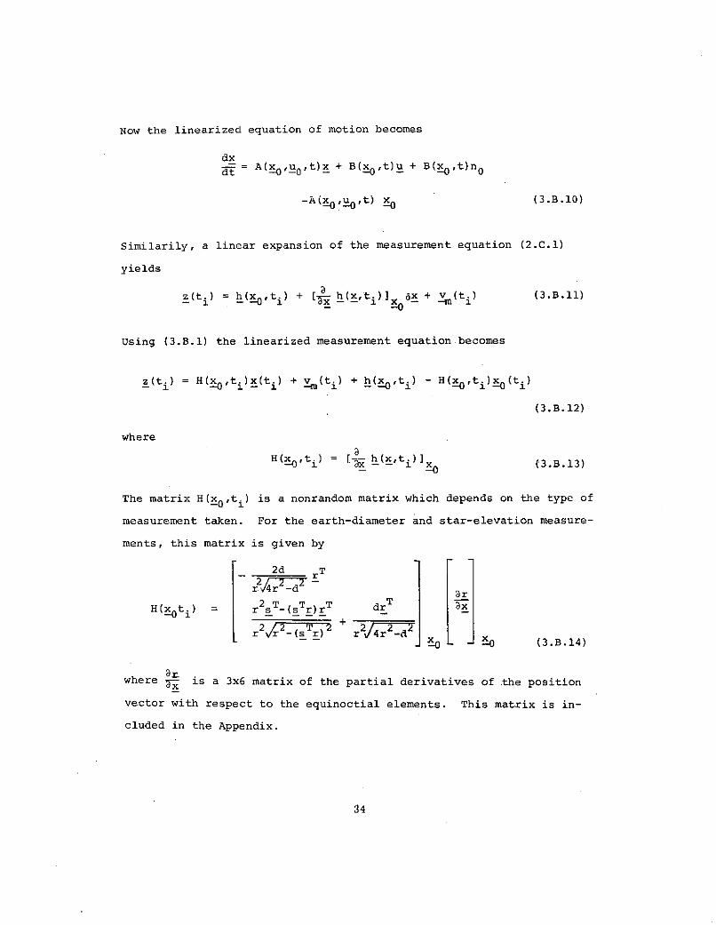
Now the linearized equation of motion becomes
dx
dt = A(xu 0 ,t) x + B(x ,t)u + B(Q,t)n0
-A(~0'u H,t) 2 (3.B.10)
Similarily, a linear expansion of the measurement equation (2.C.1)
yields
z(t) = h(O ,ti) + [_ h(x,ti)] 6x + vm(ti) (3.B.11)a K - M
Using (3.B.1) the linearized measurement equation becomes
z(t ) = H(x0,ti)x(t ) + vm(ti) + h(0,t i ) - H(,ti)x0(ti)
(3.B.12)
where
H(Eti) = [- h(x,t.)]-2x (3.B.13)
The matrix H(x,t ) is a nonrandom matrix which depends on the type of
measurement taken. For the earth-diameter and star-elevation measure-
ments, this matrix is given by
2d rT
Srar r2 -T --
H(xt i ) = r2s - (s Tr)r T dr ax
r2r 2 - J(s r)2 r214-r r r x 0 (3.B.14)
where x is a 3x6 matrix of the partial derivatives of the position
vector with respect to the equinoctial elements. This matrix is in-
cluded in the Appendix.
34
Page 35
3.C Discretization
It is more convienient to solve the guidance problem if the state
is expressed as the sum of a stochastic process R and a nonrandom
vector function b. Define R and b by the following equations
drS= A(x 0 u ,t) + B(x0 ,t)u + B(x ,t)nat -0 _= 0 - -( - (3.C.1)
b= A(x,u ,t)b - A(x0' t)x (3.C.2)
Then the state x is given by
x = x + b (3.C.3)
If the boundary condition on b is defined at the nominal final time
tf by
b(tf) = xf (3.C.4)
then x(tf) represents the deviation at the target. The corresponding
initial condition of b is given by
g(0) = -l (tf,0) + f (T,0)A(x ,u ,T)x 0 (T) dt (3.C.5)
where U(T,O) is the state transition matrix satisfying the follow-
ing equations
' (T,t) = A( ,u T) (T,t) (3.C.6)
Q(t,t) = I (3.C.7)
Using t3.C.3) the initial condition for 3 is given by
_(O) = x(O) - b(O) (3.C.8)
35
Page 36
Therefore x(0O) is also a Gaussian random vector with mean and covari-
ance given by
E[_(0)] = x(O) - b(O)
E{[x(0) - x(O) + b(0)1 [x(0) - x(O) + b(0)] } =M(O) (3.C.9)
The linearized measurement equation (3.B.12) may also be written in
terms of x and b
z(t ) = H(~ ,ti)x (t i ) + (ti) + h(2,t i ) + H(,,t i ) [b(t i ) - (ti)
(3.C.11)
Now (3.C.1) and (3.C.2) may be discretized. Let the time interval
[O,tf be partitioned into n equal subintervals
0 = t <t2<...<tn+l = tf (3.C.12)
Then the discretized equations are
x(t (+t j)(t +ft j +l +(t ,T) B(x ,T)u(T)dT + n-(j+l j+l j x +t j+ 1
(3.C.13)
b(t) = - (tf ,t )b¢( + ,T) A(, ,t)O 0 (T).dt (3.C.14)
where n0j is a zero mean white Gaussian random sequence
E 0j] = 0 (3.C.15)
tj+l
j m"j+1,) B(x ,,) NOT) B (x ,T)
S(tj+ 1 , -T) d (3.C.17)
36
Page 37
If the number n of subintervals is very large, the control u(t)
and the function u m(t) can be approximated by step functions
u(t) = u(t.) t.<t<t (3.C.18)
um(t) = Um(tj) tj t<tj+l (3.C.19)
Then the discretized equation (3.C.13) becomes
(t )=(j+t) j+lt)(t) + (tj+ltj)u(t) + (3.C.20)
where.
ft
(tj+ 1 t) jj+l (tj+,T) B( x,T)dT (3.C.21)
The control constraint equation (2.E.1) also become
< u(tj) Um(tj) j=1,2,...n (3.C.22)
3.D. Exponential Cost Criterion
In the absence of the uncertainties, the minimum time nominal
trajectory defined in section 3.A is the solution to the guidance
problem. When the vehicle is disturbed by random thrusting error,
the trajectory of its true motion will deviate from the nominal tra-
jectory. However, there is no reason to try to drive the vehicle
back to the nominal trajectory. Instead, the control sequence u(tj)
is determined to take into account the uncertainties so that the
vehicle will reach the target set at the nominal time tf with the
37
Page 38
control sequence bounded. For the stochastic system (3.C.11) and
(3.C.20) it cannot be assured that these objectives can be met.
Therefore probability measures are used to evaluate the effectiveness
of the control in acheiving these objectives and the probability that
the vehicle reaches the target and the controls stay within the bounds
is to be maximized.
S= Pr [x(t f) E Xtarget and Ju(tl)L< um(t 1 ) and...
and ju(tn) < Um (tn)] (3.D.1)
This probability can be written as an expectation if the following
indicator functions are defined
1 if I x i (tf)- .(xf) i(6xf)iI (6xf)[x(t f)i ] =if
if xi(t - (xf).i>(6xf)i
i = 1,6; i Z 4 (3.D.2)
u1(t if lu(tj),<um (t )I [u(t.)] = - -m jum- 10 if lu(t) I>u m(t)
j = 1,2... n (3.D.3)
Then the probability J 1 in (3.D.1) is the expectation of the product
of these indicator functions
J = E i=1,6 [x.(t f)] ,nu [u(t )1 (f4 j=,n m (3.D.4)
Application of dynamic programming to this problem will determine the
optimal control. The character of the control is such that maximum
thrust is utilized until the estimated state reaches the target state.
In effect the estimated state is driven to the target as quickly aspossible and the essential character of the minimum time solution is
also present in the maximum probability solution.
38
Page 39
Since the objective of the SEPS spacecraft iS to reach the
target set in minimum time, the control sequence u(t ) should
satisfy the equality in (3.C.22). There is no known general solution
for the problem of determining the control sequence to maximize
the expectation J 1 in (3.D.4) subject to the linear stochastic
system (3.C.11) and (3.C.20). The product of these indicator func-
tions will now be approximated by a exponential cost function.
J E ep I- I u (t )Lju(tj) + (x(tf)-x ) T Q (x(t )-x )] (3.D.5)
The weighting matrices L and Qf must be chosen so that each term
of the exponential function in (3.D.5) approximate the corresponding
indicator function in (3.D.4). The normalized second moments of the
indicator functions (6xf)i [x i(tf) ] are
Xf .+ (6xf ) i
[x i (tf )-(x) dx(tf) i 3f' i
i = 1,6; i / 4 (3.D.6)
The normalized second moments of the indicator functions Iu [u(tj)]
are
1 , .[( t j)]2 d ux(tj) d u (tj) d uz(t j )
S[um(t ) )]
m m5
k = x,y,zj = 1,2,...n (3.D.7)
where the integration is over a sphere with radius um (tj) . Therefore
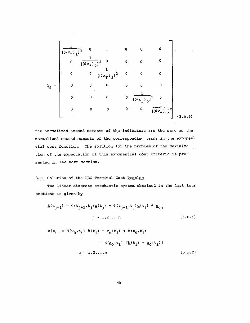
if the weighting matrices L and Qf are chosen as
Lj = I (3.D.8)
[um(t39
39
Page 40
0 [(6x f)22 0 0 0 0
10 0 x 3 2 0 0 0[(6 xf) 3]
Qf 0 0 0 0 0 0
10 0 0 0 x 2 0
[(6xf)5]
10 0 0 0 0 [(6x 612
(3.D.9)
the normalized second moments of the indicators are the same as the
normalized second moments of the corresponding terms in the exponen-
tial cost function. The solution for the problem of the maximiza-
tion of the expectation of this exponential cost criteria is pre-
sented in the next section.
3.E Solution of the LEG Terminal Cost Problem
The linear discrete stochastic system obtained in the last four
sections is given by
-(tj+l) = D(t j+'tj)x(t.) + f(tj+lt )u(t.) + nOj
j = 1,2...n (3.E.1)
z(ti) = H(x ,t i ) x(t i ) + Vm(ti) + h(x ,t i )
+ H(x,t i ) [b(t.) - (ti)]
i = 1,2,...m (3.E.2)
40
Page 41
The initial state i(tl) is a Gaussian random vector, the process
noise anj and the measurement noise m (ti) are zero mean white Gaus-
sian random sequences all of which are statistically independent.
The measurement noise covariance and the control weighting matrices
are positive definite matrices. The process noise covariance and the
terminal state weighting matrices are positive semi-definite matrices.
The problem of the determination of the controlsequence to maximize
the expectation of the exponential cost criteria in (3.D.5) is
called the linear-exponential-gaussian (LEG) terminal cost problem.
The maximization of the expectation in (3.D.5) is the same as the
minimization of the following
J2 = E y exp[- u (t )Lj u(tj) + T(t) Qf x(t)]D=l
(3.E.3)
with
y = -1 (3.E.4)
This problem is treated in a paper by Speyer, Deyst and Jacobson
[9]. The controls are restricted to be Borel functions of the past
measurement history. The key in solving this problem is to utilize
the results of the Kalman-Bucy filter [5] and dynamic programming [6].
For the terminal cost problem formulated here, the separation theorm
[11] holds. The optimal feedback control is a linear function of the
current state estimate.
u(tj) = -A(t) x(tj) (3.E.5)
where k(tj) denotes the current minimum variance estimate of x(tj).
Under the conditions of this problem, the state estimate is the
mean of x(tj) conditioned on the past measurement history [z(t 1),
z(t2 )...z(t)], ti<t.. At a measurement, this conditional mean is
41
Page 42
updated by
x(tj ) = x(tj ) + K(tj) y(tj) (3.E.6)+ ~
where x(t +) and x(t ) denote the estimate of x(t.) after and beforej j j
the measurement respectively. 'The measurement residual y(tj) is
given by
y(tj) = z(t.) - h(x,t) - H(x0,t j) [b(tj)-x(t )]
- H(x-,t ) x (tj) (3.E.7)
The Kalman gain K(t ) is given by
K(t) = P(t ) HT (~ tj) V-l(t) (3.E.8)
where P(tj) is covariance matrix of the estimation error conditioned
on the past measurement history. This conditional covariance matrix
is updated at a measurement by
P(t ) = P(t) - P(tj- ) HT(x0,tj) [H(x,tj) P(tj-) H (x,t )
+ V(t )] - 1 H(Ex,t ) P(tj-) (3.E.9)
where P(t j + ) and P(tj-) denote P(t.) before and after the measurement
respectively. Between two measurements, i(t.) and P(tj) propagate
according to the following equations
(tj+ = (tj+,t j) x(tj) + tj+1lt j ) u(t (3.E.10)
P(tj+1 ) = (t+lrt j ) P(tj+) jT(tj+lt j ) + N0j (3.E.11)
The initial state estimate and the error covariance matrix are given
by the apriori statistics of x(t ). While the separation theorm
42
Page 43
holds for this problem, the certainty equivalence principle [3] does
not hold. The feedback control gain A(t ) depends on the noise char-
acteristics. This dependence reflects the quality of the state est-
imate. The feedback control gain matrix is given by
A(tj) = [L + j+l (t+j+ j+ j+lt -T(tj+l,tj
Q(tj+l) f(tj+ ,tj) (3.E.12)
The matrix Q(tj) is given by a backward difference equation
Q(tj-1) tj'tj-1) I(t Q(j) (tjltj-1 ) [1T(tjtj-)
] j-1 j-1 j-1 j IQ(tj) (tjtj I ) + njU] -l Ttj~tj l) Q(tj)
Q(tt I 1 ) (3.E.13)
where at a measurement
Q(tj) = Q(tj ) + YQ(t j + ) K(t) [Y -l(t) - YK T(tj) Q(t + )
K(tj)]-1 K (tj) Q(t +) (3.E.14)
Note that at a measurement, (3.E.12) becomes
A(tj) = [L + T(tj+l1t j ) (t3+I ) (t j+l'tj0] - 1
jT(tj+ltj) Q(tj;l) D(tj+ltj) (3.E.15)
where Q(tj+1 ) is replaced by Q(tj+l).
The matrix Y(tj) is the covariance matrix of the measurement
residual
Y(tj) = H(x,tj) P(tj) HT (,t) + V(tj) (3.E.16)
43
Page 44
Equation (3.E.14) shows the dependance of the control gain matrix on
the noise characteristics explicitly. The terminal condition of
Q(tj) is given by
Q(tn+ ) = f + yQ I[P l(tf +) - YQf ] Qf (3.E.17)
3.F The Guidance System
The linear feedback control law obtained in the solution of the
LEG terminal cost problem can be used for the midcourse guidance of
the SEPS Spacecraft. Since the overall objective of the SEPS Space-
craft is to reach the target set in minimum time, full thrust acceler-
ation will be used to propel the vehicle. The LEG guidance law is
used to determine thrust direction only and full thrust magnitude is.
always utilized. Therefore the guidance law is given by
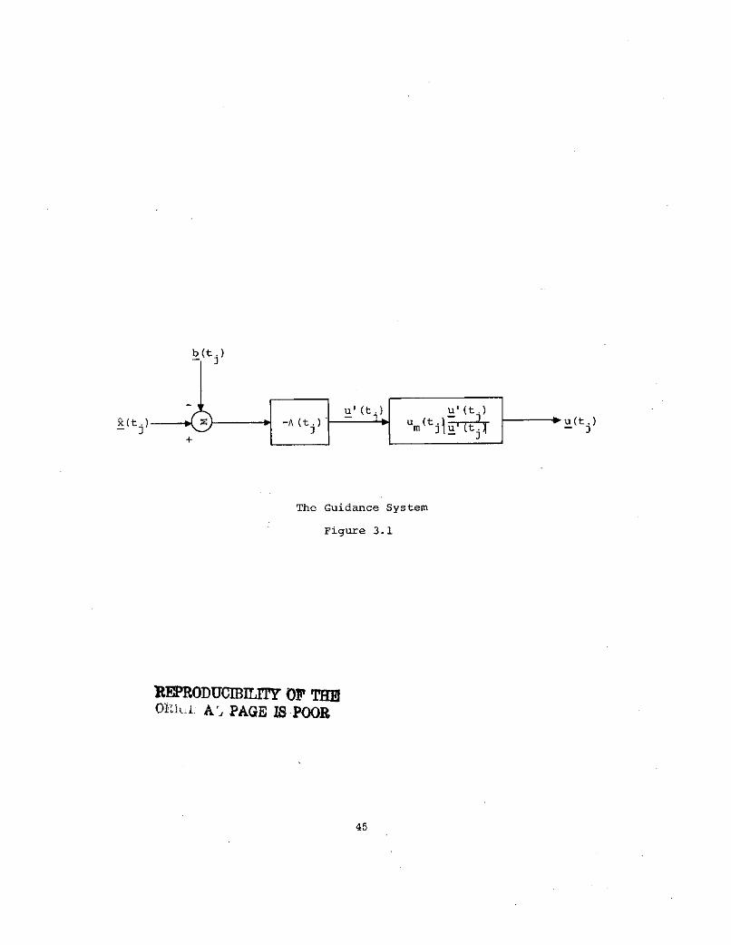
u'(t.)u(t m(tj) j I (3.F.1)
where using (3.C.2) and (3.E.5) u'(tj) is given by
u'I(t ) = -A(tj) [^(tj) - b(tj)] (3.F.2)
The on-board guidance system is only required to perform the vector
subtraction and matrix multiplication in (3.F.2). The feedback
control gain matrix A(tj) and the vector b(t ) can be computed be-
fore the mission and stored in a computer on the SEPS for real time
mission usage. The navigation system to estimate the state x(tj)
is discussed in the next chapter. The guidance law (3.F.2) is
pictured in Figure 3.1.
44
Page 45
b (t-
(tj) -A (t ) m(tj u(t
The Guidance System
Figure 3.1
REPRODUCIBILTY OF THFOrihi. Al PAGE IS1POOR
45
Page 46
CHAPTER IV
THE NAVIGATION SYSTEM
In the last chapter a linear feedback control law was obtained
for the guidance of the SEPS Spacecraft. Using this control law, the
vehicle will fly in a trajectory neighboring the minimum time nominal
trajectory. Therefore the linear Kalman filter presented in section
3.E is not adequate to estimate the vehicle's state. In this chapter
the extended Kalman filter [7] which is adequate for neighbouring
trajectory estimation is discussed. This estimator, together with the
linear feedback control law obtained in the last chapter forms the
complete closed-loop midcourse guidance and navigation system for
the SEPS Spacecraft.
4.A Extended Kalman Filter
The extended Kalman filter has the same structure as the linear
Kalman filter. However, instead of linearizing about the minimum
time nominal trajectory alone, the extended Kalman filter is linear-
ized about a number Of nominal trajectories.. After each measurement,
a new estimate of the state is obtained. This new estimate is used
to define a new nominal trajectory. Then the equation of motion and
the measurement equation are linearized about this new nominal tra-
jectory.
It is more convenient to discuss the extended Kalman filter if
the continuous equation of motion (2.B.1) is used. Now suppose the
control u(t), O<t<tf is known. Let the estimate of the state and the
error covariance matrix of this estimate after the measurement at
PRECEDING PAGE BLANK NOT FILMED47
Page 47
time ti be x(t') and P(t') respectively. This estimate is used to- .1
define a nominal trajectory xi(t) by
dxi (t)dt - G (x.,t) u(t) t.<tdt 1 - (4.A.1)
xi(ti) = x(t) (4.A. 2)
The subscribt i is used to emphasize the dependence of the nominal
trajectory xi(t) on the state estimate x(t i ). Define ?6x(t) and
6z (ti+1 ) by
6x (t) = x(t) - xi(t) t <t(4A3)
6z (ti+ ) = z(t i+) - h(x ,ti+ I ) (4.A.4)
Linearization of (2.B.1) and (2.C.1) about this nominal trajectory
yields
d6x (t)t - = A(x.i u ,t ) 6x.(t) + 3(x.,t)n t.<t (4.A.5)
6.(ti+l) = H(xi,ti+) 6x.(ti+ ) + v (ti+l) (4.A.6)-( 1+ -H t1+1 - 1+1 -m i+1
Now the linear filtering theory can be applied to estimate 6x.i(t).-1
Before the measurement at time t.i+ the estimate 6xi(t) and the
error covariance matrix P6x.(t) of this vector are given by the-1
following equations
d6:i (t)dt_- A(x.,u,t) 6x.i(t) (4.A.7)
dP~x (t)-1-1-dt = A(x.,u,t) P (t) + P (t) A (x .,u,t)
dt -1 6i 6x -1
N BT! ,t
+-i'-)N T . ,t) tit<ti+l (4.A.8)
48
Page 48
Using (4.A.3) this estimate is related to the estimate ~(t) of the
state x(t) by
68i(t) = _(t) - x.(t) t.<t (4.A.9)-1 - -1
Also using (4.A.2)
62. (t+ ) = 0 (4.A.10)-1 1
and in view of (4.A.7)
6Ei(t) 0 t <t<ti+ 1 (4.A.11)
Therefore before the measurement at time ti+, the estimate of the
state is given by the nominal trajectory xi(t)
- (t) = x(t) (4.A.12)S -
dx(t) = G(x,t) u(t)dt
t i<t<ti+l (4.A.13)1- i+l
At the measurement at time ti, 6x(t) and P (t) are updated by the+11 6x.-i
following equations
6 (ti+ ) 6 i+ (t K (ti 6zi(ti+ ) - H(x ,ti+
6x. (t. )} (4.A.14)-1 1+1 -
K.(ti+l) = P (t+l H T (xt ) V 1 (ti ) (4.A.15)1 1+1 6x i+1 i.1 i+l i+l
-1
6x i+l -1 i+l 6x i 1+1 i+l+ -
P (t ) H T(x,ti+) + V(ti+1)] H(x ,ti+ 6x. i+lx +l i i +l i+l -I- t +1 P (t
-(4.A.16)
49
Page 49
Using (4.A.4), (4.A.9), (4.A.11) and (4..A.12), (4.A.14) becomes
x(t ) = (t ) + Ki(ti ) {z(t ) - h[x(t ),t +]}i+1 i+l i i+1 i+1 i+l i+l
(4.A.17)
Using (4.A.3) the error covariance matrix Px. (t) of the estimate of-
6xi(t) and the error covariance matrix Pi(t) of the estimate of x(t)
are the same
dP i (t)d -t) A(,u,t) P.(t) + P.(t) AT(,u,t) + B(x,t)N BT(,t)dt - t 2 x
ti <ti+l (4.A.18)
Pi (t+ Pi(ti+ Pi H (ti+l ]{H[(t ),tii -i+l i+1+
)i+ ' i++V(t )}-1 H[x(t ),ti+ Pi (i+
(4.A.19)
Hence (4.A.17) can be rewritten as
(ti+l (i+ ) + Ki(ti+ ) {z(t ) - h[x(t ),t ]}i+l i+i+l i+l
(4.A.20)
where now the Kalman gain Ki(ti+l) is given by
HT [(t )t t (4.A.21)Ki(ti+ = Pi(ti+) H [x(t i+ ] i+) (4.A.21)
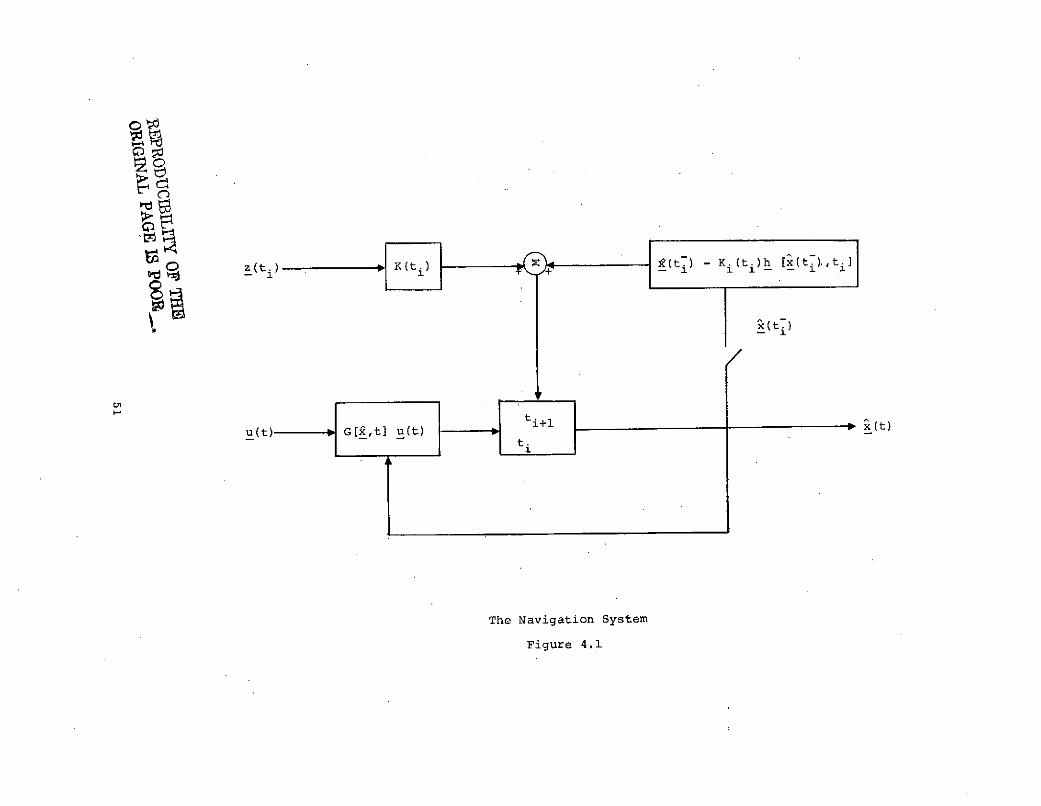
Now the new estimate x(t + ) can be used to define a new nominali+1
trajectory similar to (4.A.1) and (4.A.2) and the preceding method
can be repeated. The result is the extended Kalman filter given by
(4.A.13), (4.A.18) to (4.A.21). This estimator is pictured in
Figure 4.1.
50
Page 50
- (t K) - K (t)h [x(t ti
u(t) G[i,t] u(t) i+lti
The Navigation System
Figure 4.1
Page 51
4.B The Closed-loop Guidance and Navigation System
The linear feedback control law in Chapter 3 and the extended
Kalman filter in the last section forms the complete closed-loop
midcourse guidance and navigation system for the SEPS Spacecraft.
The on-board guidance system consists of the linear feedback control
law (3.F.1) and (3.F.2) where A(tj) and b(tj) are precomputable
quantities. Note that A(t ) is computed by using the equations in
Chapter 3 where the quantities P(t ) and K(t ) are not the same as
the quantities Pi(t) and Ki (t) in the last section. The quantities
P(tj) and K(tj) are computed along the minimum time nominal traject-
ory while the quantities Pi(t) and Ki (t) along a number of nominal
trajectories. This control law will guide the vehicle to fly along
a trajectory neighbouring to the minimum time nominal trajectory
and reach the target set at the nominal final time tf. The thrust
acceleration is always fully utilized to propel the vehicle and the
control is always on the constraint boundary for this minimum time
mission. The on-board navigation system consists of the extended
Kalman filter (4.A.13) and (4.A.18) to (4.A.21) where all the quanti-
ties must be computed on-board the vehicle. The on-board computa-
tion of these quantities is the most important disadvantage of this
navigation system. The closed-loop system is pictured in Figure 4.2.
Although this guidance and navigation system is designed for the mid-
course phase, it can also be used for the terminal phase by including
the term for the angular position of the vehicle in the terminal
state weighting matrix. However, in this case the objective of
reaching the target set which now included the angular position of
the vehicle is more difficult to meet than the midcourse case, unless
the nominal mission time is very short.
52
Page 52
z(t)
u(t)
)- i (ti)h[x(t7) 1 t il z (t
b(t)R(t )
I_ u'(t) + + xtt) I fti+l
Us u t x)ti+dt G[x,t]u(t)
The closed-loop System
Figure 4.2
Page 53
CHAPTER V
SIMULATION RESULTS AND DISCUSSION
A computer program has been prepared to simulate this midcourse
guidance and navigation system in real time. Although the system
was originally designed for missions from near earth orbits to geo-
synchronous orbits, the simulation of a shorter mission should
equally well reveal the character and performance of the system.
The simulation results of this short mission, together with a dis-
cussion are presented in this chapter.
5.A Simulation Results
The minimum time deterministic control problem which generates
the minimum time nominal trajectory defined in Section 3.A can only
be solved by numerical methods. For the simulation in this research
an approximate minimum time nominal trajectory is used. For the de-
tails of this approximate minimum time trajectory, the reader is
referred to Shepperd [7]. Flying along this nominal trajectory the
SEPS Spacecraft would reach the desired geosynchronous orbit from a
near earth orbit. If the near earth orbit has a radius of 4300 miles
and an inclination of 28 degrees, and if the desired geosynchronous
orbit has a radius of 2600 miles and an inclination of 0 degrees, the
nominal final time of this mission would be approximately 150 hours.
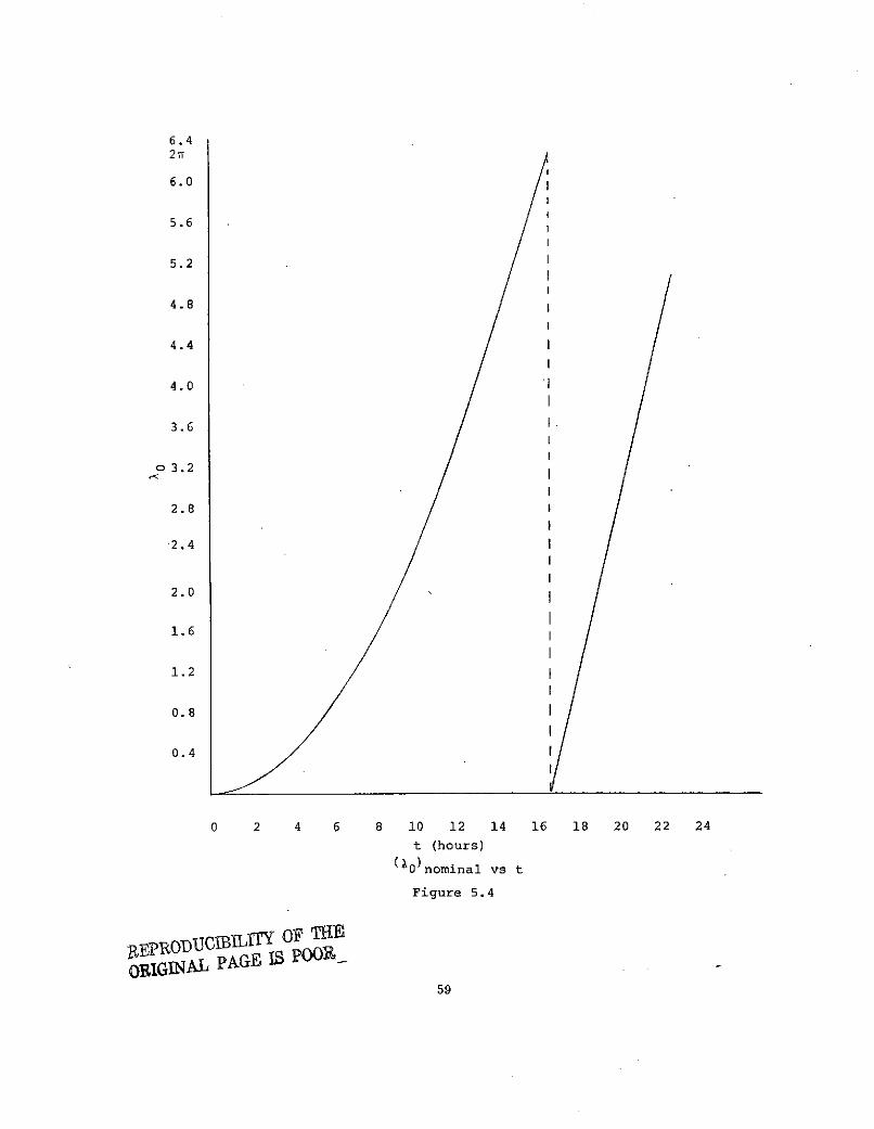
In the results presented here only the first 22.64 hours of the mis-
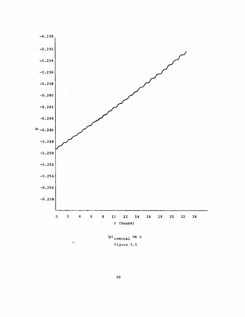
sion are simulated. This nominal trajectory is pictured in Figures
5.1 to 5.6. The semi-major axis is increasing approximately linearly
with time. This shows that the averaged radius of the orbit is in-
PRECEDWG -PAGE BLANK NOT 55
Page 54
1.36
1.34
1.32
1.30
1.28
1.26
1.24
- 1.22--4-,4
s 1.20
0 1.18
1.16
1.14
1.12
1.10
1.08
1.06
0 2 4 6 8 10 12 14 16 18 20 22 24
t (hours)
(a)nominal vs t
Figure 5.1
5,6
Page 55
0.7
0.6
0.5
0.4
0.3
0.2
0.1
-4 0.00.0
-0.1
-0.2
-0.3
-0.4
-0.5
-0.6
0 2 4 6 8 10 12 14 16 18 20 22 24
t (hours)
(h)nominal vs t
Figure 5.2
57
Page 56
0.7
0.6
0.5
0.4
0.3
0.2
0.1
4 0.0
-0.1
-0.2
-0.3
-0.4
-0.5
-0.6
0 2 4 6 8 10 12 14 16 18 20 22 24
t (hours)
(k) nominal vs t
Figure 5.3
58
Page 57
6.42 rr
6.0
5.6
5.2
4.8
4.4
4.0
3.6
03.2
2.8
2.4
2.0
1.6
1.2
0.8
0.4
0 2 4 6 8 10 12 14 16 18 20 22 24
t (hours)(10)nominal vs t
Figure 5.4
OD B OF TH5ORIGINAL PAGE IS IOOB
59
Page 58
-0.230
-0.232
-0.234
-0.236
-0.238
-0.240
-0.242
-0.244
-0.246
-0.248
-0.250
-0.252
-0.254
-0.256
-0.258
0 2 4 6 8 10 12 14 16 18 20 22 24
t (hours)
(P)nominal vs t
Figure 5.5
60
Page 59
0.24
0.22
0.20
0.18
0.16
0.14
0.12
0.10
~0.08
0.06
0.04
0.02
0.00
-0.02
-0.04
0 2 4 6 8 10 12 14 16 18 20 22 24
t (hours)
(q) nominal vs t
Figure 5.6
;?EPRODUCIIBLITY OF THORIGINAL PAGE IS POOR 61
Page 60
creasing. The equinoctial elements h and k vary sinusuidally with
an increasing amplitude. This increasing of amplitude showed that
the averaged eccentricity of the orbit is increasing. The equinoc-
tial element 10 is increasing monotonically from 0 radians to
(27 + 5.073) radians. This variation showed how the angular posi-
tion of the SEPS Spacecraft in the orbit is changed by the engine
thrust acceleration. Finally the variations of the equinoctial
elements p and q showed that the inclination of the orbit is de-
creasing monotonically.
The values of the input variables used in this simulation are
summarized as follows. The statistics of the initial state are
0.1085 x 10'er
0.0
S 0.0x(0) =
0.0
-0.249
0.0(5.A.1)
-5 2 -5 -220.196x10 er 0.0 0.169x10 er 0.0 er -0.153x10 2 2 er
0.0 er 0.139x10- 5 0.0 0.143x10- 5 0.0
0.169x10⁻⁵er 0.0 0.150x10- 5 0.0 -0.414x10- 2 3
0.0 er 0.143x10 - 5 0.0 0.154xl0- 5 0.0
-0.153x10⁻²² er 0.0 -0.414xl0 - 2 3 0.0 0.6102x10- 7
_0.0 er -0.161x10 - 2 2 0.0 0.480x10 -7 0.0
0.0
-0.161x10- 2 2
0.0
0.480xl0- 7
0.00.0 ] (5.A.2)
0.103x10- 6
62
Page 61
where er is earth-radii
er = 0.20925696 x 10 feet (5.A.3)
The vector x(0) is equivalent to a circular orbit with a radius of
4300 miles and an inclination of 28 degrees. The matrix m(0) is
equivalent to the following standard deviations
(a ) = 1 mile (5.A.4)rl
(or 2 = 5 miles (5.A.5)
(r) 3 = 1 mile (5.A.6)
(a ) = 5 feet/second (5.A.7)
(G )2 = 15 feet/second (5.A.8)
(G )3 = 15 feet/second (5.A.9)
where (r) 1 , (Or)2' (Or) 3,(Yv)1 , (0)2' (Ov)3 are the standard,
deviations of position and velocity in altitude, down range and
cross track directions respectively. These statistics are typical
of a spacecraft launch trajectory. The nominal final time is
tf = 22.64 hours (5.A.10)
The parameters defining the target set are
0.1329x10'er
0.2670xl0- 2
0.3221x10⁻²
f = 0.5073x101
-0.2325
-30.2068x0 3 (5.A.
63
Page 62
(6xf) 1 = 0.775 x10⁻⁴er (5.A.12)
(6xf) 2 = 0.858 x10- 4 (5.A.13)
(6Xf)3 = 0.971 xl0- 4 (5.A.14)
(6x )5 = 0.594 xl0- 4 (5.A.15)
(SXf) 6 = 0.106 xl0- f (5.A.16)
The values of the parameters 6xf defined the size of the target
set. Since it is expected that the deviation between the true and
nominal state at the nominal final time will not be less than the
expected estimation error, the values 6xf in (5.A.12) to (5.A.16)
are taken from the standard deviations of the corresponding diagon-
al elements of the estimation error covariance matrix P(tf). Note
that the covariance matrix P(tf) is computed along the minimum time
nominal trajectory which is not the same as the covariance matrix
Pi(tf) computed using the equations of the extended Kalman filter.
The thrust acceleration function is
Cg0u m(t) =
U (I (5.A.17)s
where g0 is the surface gravity acceleration, Is is the engine
specific impulse and e is the engine's initial thrust acceleration
in terms of the g0's
E = 0.1 xl0- 2 (5.A.18)
I = 0.4 xl0 4 sec (5.A.19)
g0= 32.0 feet/second2 (5.A.20)
The parameters which represent the strength of the process noise are
N1 = 0.1 x10- 3 (5.A.21)
N, = 0.42 x10 - 7 (5.A.22)
64
Page 63
The value of the parometer N 1 in (5.A.21) is equal to the square
of 1 percent and the value of the parameter N 3 in (5.A.22) is equal
to 1/2 of the square of 1/60 degree. A set of measurements is
taken every half orbital period. Each set of measurements consist
of one earth-diameter and two star-elevation measurements. The
parameter which represents the strength of the measurement noise is
.84x10-7 0 0
Vi = 0 0.84x0 - 7 0
0 0 0.84x10-I (5.A.23)
Note that (0.84x10⁻⁷) is equal to the square of 1/60 degrees
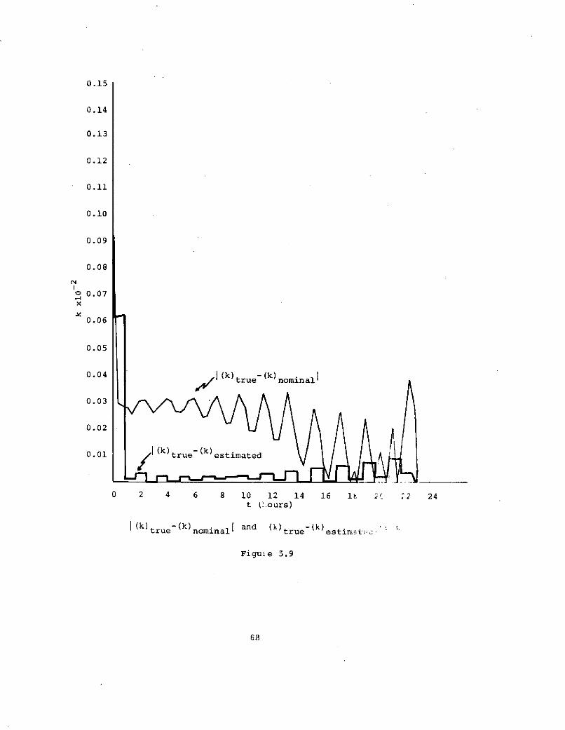
The results of this simulation are pictured in Figures 5.7 to
5.12 where the difference between the true state and nominal state,
the difference between the true state and the estimated state as
shown. At the nominal time tf, the results are
-40.9232 x 10 er
0.7592 x 10 - 4
-0.4034 x 10 - 4
x(t ) true - (t nominal = -0.6880 10
-0.2113 x 10⁻⁴
0.6884 x 10 - 4 (5.A.24)
-30.1796 x 10⁻³er
-30.1423 x 10-
0.6247 x 10 - 4
x (tf)true - x(tf estimated 0.1330 x 10-0.1330 x 10
0.3895 x 10- 4
0.1145 x 10 - 4 (5.A.25)
65
Page 64
0.15
0.14
0.13
0.12
0.11
0.10
0.09
- 0.08
o I (a)x 0.07 (a)
(u 0.06
0.05
0.04
0.03
0.02
(a) true- (a) estimated0.01
0 2 4 6 8 10 12 14 16 18 20 22 24
t (hours)
I(a) true- (a) nominall and I (a) true- (a) estimated vs t
Figure 5.7
66
Page 65
0.30
0.28
0.26
0.24
0.22
0.20
0.18
0.16
00.14 (h) true
x )nominall
0.12
0.10
0.08
0.06
0.04
(h) true-(h) estimated
0.02
0 2 4 6 8 10 12 14 16 18 20 22 24t (hours)
I (h) true- (h) nominall and (h) true- (h) estimatedl vs t
Figure 5.8
67
Page 66
0.15
0.14
0.13
0.12
0.11
0.10
0.09
0.08
o 0.07x
0.06
0.05
0.04 (k) true- (k) nominal
0.03
0.02
0.01 (k) true- (k) estimated
0 2 4 6 8 10 12 14 16 It '. 22 24t (::ours)
1(k) true- (k) nominal and (k) true-(k) estimt.
Figu.e 5.9
68
Page 67
0.08
0.07
0.06
0.05
0.04
(0) true
-(X) nominal0.03
0.02
0.01
0) true-0 estimate
0 2 4 6 8 10 12 14 16 18 20 22 24
t (hours)
I (0G)true- 0 ) nominal and I 0 O true-( o0estimated' Vs k
Figure 5.10
69
REPRODUCIBILITY OF THEORIGINAL PAGE-IS POOR
Page 68
0.30
0.28
0.26
0.24
0.22
0.20
0.18
0.16
0 (P) true P) nominalo0.14
0.12
0.10
0. 08I ( )t rue
0.06 -(P) estimated
0.04
C 2 4 6 8 10 12 14 16 18 20 22 24t (hours)
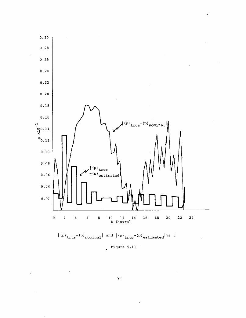
I (P)true-(P)nominalI and I(P)true-(P)estimatedvs t
Figure 5.11
70
Page 69
0.60
0.56
0.52
0.48
0.44
S(q) true
0.40 - ( q ) nominal
0.36
l 0.32
00.28
0.24
0.200.0I (q)true- ( q ) e s t i ma t e
0.16
0.12
0.08
0.04
0 2 4 6 8 10 12 14 16 18 20 22 24
t (hours)
(q) true- (qnominal and (q) true-(q)estimatedj vs k
Figure 5.12
71
REPRODUCIBILr OF p 2ORIGINAL PAGE IS POOR
Page 70
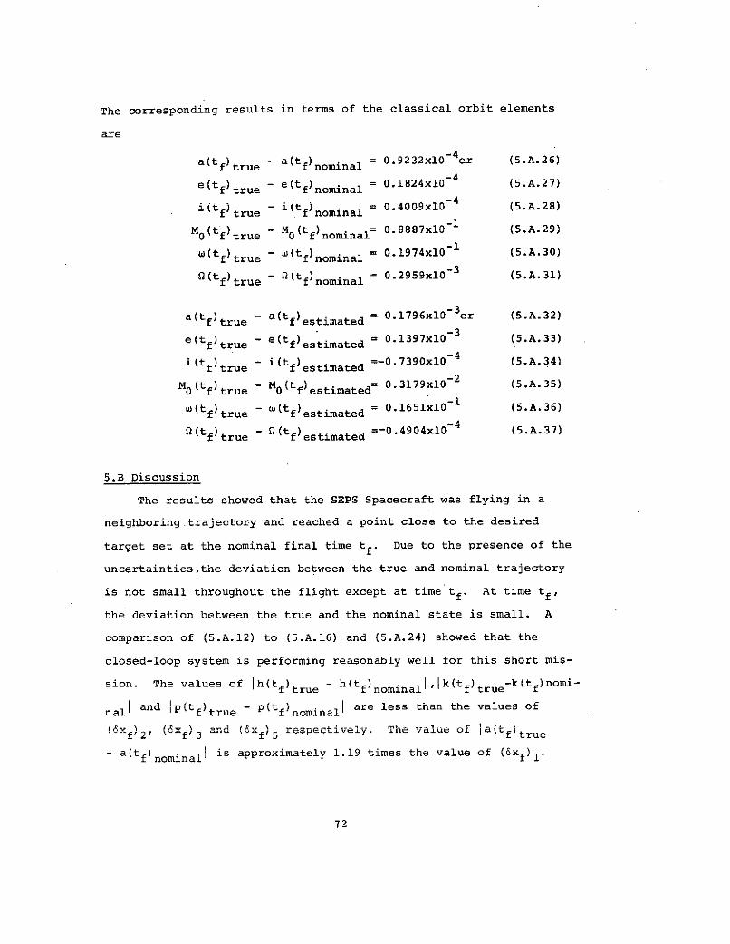
The corresponding results in terms of the classical orbit elements
are
a(t ) - a(t) nominal 0.9232x10 4er (5.A.26)f true f nominal
-4e(tf)true - e(t ) = 0.1824x10 (5.A.27)
M0( t f t r u e - M ( t f n o m i n a l 0.8887x - (5.A.29)i(t ) - (t )nomina = 0.4009x10 (5.A.28)f true f nominal
Mg(tf)true - (tf)nominal = 0.29598887x10 - 1 (5.A.3129)-1w(t f)t - w(t ) 0.1974x10 (5.A.30)f true f nominal
-3
(t )tr - (t ) = 0. 197x10 - (5.A.32)-3a(tf)true - a(tf)estimated 0.1796x10er (5.A.32)
e(tf)true- e(tf)estimated 0.1397x10 3 (5.A.33)
0 ( t true - M0 (testimated = 0.3179x10⁻² (5.A.35)
w(t )true - W(t) estimated= 0.1651xl0- (5.A.36)f true f e s t i m a t e d
-4(tf) - (t) estimated=-0.4904x10 4 (5.A.37)
true f e s t i m a t e d
5.3 Discussion
The results showed that the SEPS Spacecraft was flying in a
neighboring.trajectory and reached a point close to the desired
target set at the nominal final time tf. Due to the presence of the
uncertainties,the deviation between the true and nominal trajectory
is not small throughout the flight except at time tf. At time tf,
the deviation between the true and the nominal state is small. A
comparison of (5.A.12) to (5.A.16) and (5.A.24) showed that the
closed-loop system is performing reasonably well for this short mis-
sion. The values of Jh(t )true - h(tf)nominall ,k(tf)true-k(tf)nomi-
nall and ip(tf)true - P(tf)nominall are less than the values of
xf, 2, (xf) 3 fand 1x f 5 respectively. The value of ja(tf )true
- a(tf)nominalI is approximately 1.19 times the value of (6xf)1'
72
Page 71
The value of Jq(t f)true - q(tf)nominal is approxiamtely 64.94 times
the value of (6xf)6. This large ratio is due to the fact that (6xf)6
is very small and the actual estimation error [q(tf )true - q(tf)esti-
matedl is approxiamately 10.6 times the value of (6xf)6 . However,
since the equinoctial elements p and q should have the same charac-
ter, a comparison of the values of Ip(tf)true - P(tf)nominall and
9q(tf)true - q(tf)nominall in (5.A.24) showed that the closed-loop
system is still performing reasonably well. The value of (10 )true
- ("0)nominalI is not small for this midcourse flight since this
equinoctial element is not included in the exponential cost criterion.
The deviation between the true and estimated state is also pre-
sented in Figures 5.7 to 5.12. Between two measurements the estima-
tion errors are approximately constant. At a measurement the esti-
mation errors have discontinuities. These estimation errors tend
to increase slowly with time. This indicated that for a longer mis-
sion some more accurate measurements such as ground based tracking
must be used to reduce these estimation errors. At these high ac-
curacy ground based measurements,the minimum time nominal trajectory,
the feedback control gain matrix A(tj) and the vector b(t ) could
also be updated. If these ground based updates are included in the
miscourse guidance and navigation of the SEPS Spacecraft, the closed-
loop system developed in this research should also perform well for
a longer mission.
The most important advantage of using the LEG guidance law in
the closed-loop system is that the weighting matrices Lj and Qf can
be chosen to achieve desired system performance. This fact is indi-
cated by the simulation results. In the linear-quadratic-gaussian
(LQG) problem [1], these weighting matrices usually must be obtained
by iterations to achieve the desired system performance.
73
Page 72
CHAPTER VI
CONCLUSIONS
A practical and efficient midcourse guidance and navigation sys
system for the SEPS Spacecraft has been developed in this research.
To reach the target set in minimum time the SEPS Spacecraft always
utilizes full thrust magnitude. The thrusting direction of the en-
gine is determined by the solution of the LEG terminal cost problem.
The LEG approach provides a systematic way of determining weighting
matrices for problems involving bounds and the control system design
did not require many iterations, as is typically the case when the
LQG approach is used. The solution of this problem, which is the
guidance law, determines the control as a linear function of the
current state estimate. Using this guidance law, the SEPS Space-
craft will fly in trajectory neighbouring the minimum time traject-
ory. To take into account this fact, the extended Kalman filter is
used for the navigation of the SEPS Spacecraft.
The simulation results of a short mission have indicated that
this closed-loop system is very efficient in bring the SEPS Space-
craft to the target set. However, these results have also indicated
that the state estimation errors tend to increase slowly with time.
For a long mission this means that the navigation system would have
very poor state estimation and consequently the closed-loop system
would have very poor performance. Therefore it is concluded that if
this system is to be used effectively for a long mission, some more
accurate ground based measurements and nominal trajectory updates
must be included in the guidance and navigation of the SEPS Space-
craft.
75
'PRWEDIqNG PAGE BgLAN NOT PI
Page 73
The determination of an efficient measurement schedule, the fre-
quency of high accuracy ground based measurement and nominal tra-
jectory updates can be carried for further study to improve the
effectiveness and performance of this closed-loop system. The pos-
sibilities of using this closed-loop system for terminal guidance and
navigation of the SEPS can also be investigated.
76
Page 74
APPENDIX A
axTHE MATRIX ar
axThe matrix 7 is given by
ax aT ahT T axT T qT] (A-l)
5r 1r ' r ar ar (A
where
T 2aa a r (A-2)
r 3- r
hT /l-h2-k 2 X 1 a3 Y 3h [ (--- + hm X )f + ( + h~m a Y1)g]3r 2 k 3 1 k 3
ma r r
k(ql-p k 1) w (A-3)2 22
ma 2 /l-h 2-k2
T 22 Xl a 3 Y 3k 1-h -k a 1 ar - 2 - km 3 Xl)f + ( - km 3
- ma r r
h(q~i-pk1)
+ - w (A-4)
ma 2 /1-h 2 -k 2
aoT 22 aaa 0 1 31it /1-h2-k2 1
D - -(- 3 2 8[(h + k -- ma r ma
S 1Y (qYI-PX 1)+ (h - + k k - )g] - w (A-5)2 2 .-
ma /1-h -k
77
Page 75
T 22= 1+p2 +q2 (A-6)
ma2 /1-h2k
T 2 2_ 1+p +q Xw (A-7)
- ma2 1-h-k 2
h1 T f (A-8)
aX1 Tv f (A-9)Tk- ( )
aYl av1 - T (A-10)
S(-) g (A-)k k
av av
The partial deriviatives , are presented in Appendix C.
78
Page 76
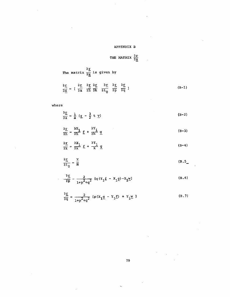
APPENDIX B
arTHE MATRIX --
ax
The matrix a is given byax
3r ar 3r 9r 3r Dr ar_ = I - (B-l)
x aa -3F k ax 0 p aq
where
r 1 (r tv3 ) (B-2)a a 2
r a a (B-3)=h - f + 3F g
ar aX 1 Y- 3 f + - g (B-4)
r v(B.5
ax 0 m
2 2 [q(f - Xg)-X] (B.6)
1+p +q
r 2 [P(Xlg - Yf) + Y 1 w ](B.7)+p2 +q2
79
Page 77
APPENDIX C
avTHE MATRIX -
avThe matrix - is given by
av av av av av av @vx = I =- =- = (C-l)
where
1 (V - ) (C-2)a 2a r 3
= f + g (C-3)
ak f+ -g (C-4)
av 3- -m r (C-5)
ax0 r
S[q( - 1g ) - X w ] (C-6)+p 2+q2 -
av 2= [p(1g yl ) + Yl w ] (C-7)aq l+p q
1 _ ma 2 h28 + 3ah a 2h r 2 - + ) (1- ) a cos F(X-F) + ha sin F + F cos F]
Xa1 a cos F (X-F) - sin Fl (C-8)r r
81
tf11ADN OT ,R VL
Page 78
ma hk (1 r) + ah sin F (X-F) + cos F (h.-- sin F)]- r - a r r
aX1 a si
+ 1 [ sin F (X-F) + cos F] (C-9)r r
ai m2 hk83 r aakama2 hk -1) + ak cos F (X-F) - sin F (kB - a cos F)]
= 1-8 a r r
aY ar [ cos F (X-F) - sin F] (C-10)
r r
= ma 2 k 2 -3 1) ak - sin F(X-F) - k8 cosF - sin F]
aY1 a+ - -- sin F(X-F) + cos F] (C-11)
r r
= X0 + mt (C-12)
82
Page 79
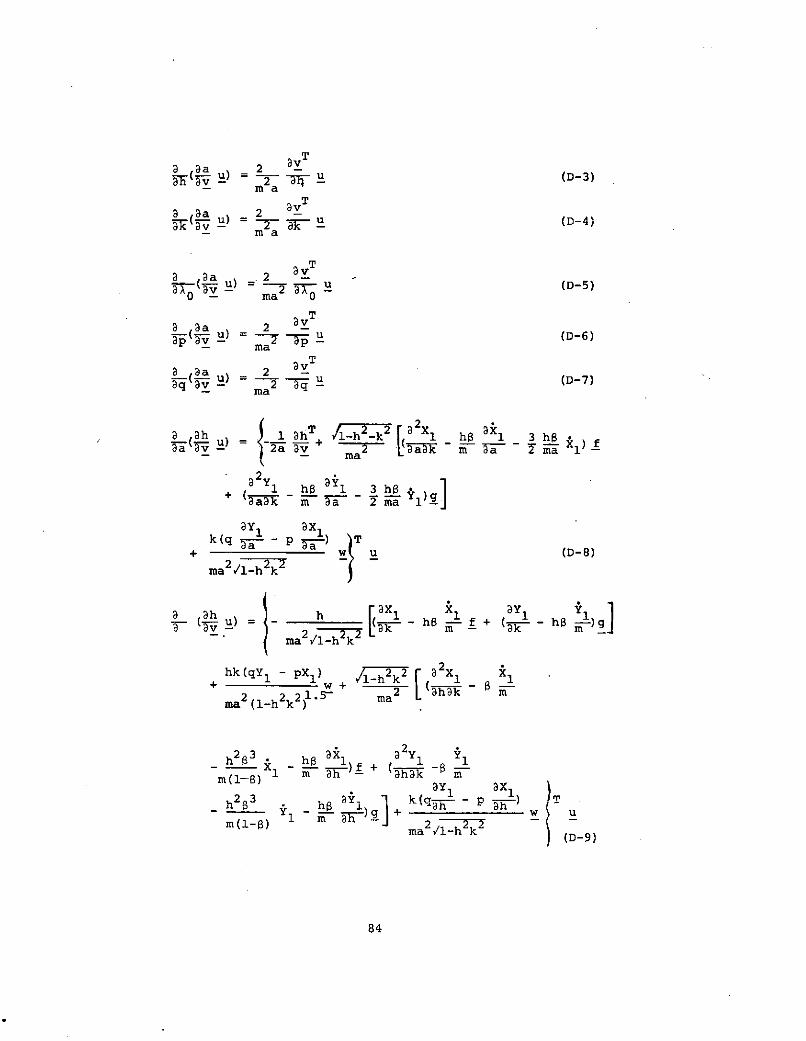
APPENDIX D
THE MATRIX A(x 0 , u0 t)
The matrix A(x 0, u 0 , t)is given by
A(x 0, uO' t) = [ G(x,t)u]x0
S a ) a a a a 3a a aa a 2(a uSaa ) u) ) o_ , u _
a ua a u) l a a u a a a a
Su) ~ u) b" u ) ,( u ) ,u) 2U)
7 -- -) a €v -- u -_) Wk 3v-Uav ) ap --_ u
u) u) a( u) o( u) ( u) U)
av- ahav v- ax av apav - av-
aa av ah a)v a av av a
a a 4a 2a (D-2)- -au ) = (v ' -) u a(D-2
83
Page 80
a aa 2 (D-3)av- u) - u (D-3)- ma
vT
8 a 2 -a (-a u) = 2 -k U (D-4)- ma
T
avTS a 2 a -(D-5)a 0 - ma 0
_ = -- u (D-6)- ma
a a =2 T=q v- ma2 (D-7)
a h1 aI /+ A-h 2-k 2 2x 1 hB a X1 3 hB) = -2a m 2 UaW m Ba 2 ma X)f
1 ha 1 3 h+ (~ m Ba 2 ma -
ay1 ax1k(q 5 - p (D-8)
ma 2/1-h2 k2
a3h h aX 1 X1 1 1a- u) = h[ x h f + (- h -)ga v f 2 - 2 ak F- mk
-_ (ma /1-h k
hk(qY 1 - PXl) k 2 32X X1+ + 2 (3hk -
ma 2 (1-h2k2)1. -ma
h2 3 h X1 a 1 1
m X(1-) 1 m 7h ahak m
,2,3 - y ' k1n- 1 - ) ,i1 h + ahh P a
m(1-8) ma2/1-h 2 (D-9)
84
Page 81
aX X kY [ 1 1)1S ) = k (a - h )f + ( - h m1
- ma2/-h2k
(1-h2) (qY1 -pX 1 ) 1-h 2 k 2 3a2X1 hk 3 X h h 12 2m2 1ma [ m -
ma2 (1-h2k2 1.5 ma k
2a2y 1 hkB 3
h 1+ ( 2 - m k)gak2 m(1-) 1 m k)
k y 1 axlk(q k p ) Tma2 k w u (D-10)
a h /1-h k 1 ha 131 --- = h6 jiFk m aho ay ma 0
k(qY - Px) w kX 1(q )+ ax'_ 2,__2 l-h- a2 l -2 u (D-12)
-h 2 k2 ma /1-h-k
a- u) = /1h--k ( h6-) + ( hB )-p- a ma
k(qY - pX1) aw k 1
2 ~2 2a
ma 2 1-h-k 2 ma2/ 1-h-k 2
(2 u)= 1-h k _ _ ha 1 1 hl -)v- ma 2 k m aq @k m ap
k(qY1-pX1) aw+ kY1
2/ - + w u (D-13)
ma2 m 1-h -k2
85
Page 82
a Sk _ 1 kT - -h2 -k2 Xl k 15 u a - 2a I 9a + i*
-ma
+3 kB 2 Y1 k8 I 3 kB2 ma 1 -+ (aaah m aa 2ma 1
ay1 ax1
- p a-) w u (D-14)
ma /1-h -k2
a @k h ax1 1 1 1l, Y)m ah m
ma 2 /1-h 2 -k 2
(1-k2) (qY1 -pX) 1-h 2 -k 2 + hkB
2 ma 2h 2 3
ma2 (1-h2-k2 3/2 ma h m(-8)
k Xl a 2Y1 hk83 " kB 1m 3a 21 2 m h _
m 3a 3h m(1-) + m gaY ax1qY 1 1 T
3F w u (D-15)
na2/1 -h 2-
k 2
S 3k uk ax1 x aXl 1 Y1- ( u)= ( + k-) f + + k -)
2 2 2 2 kma (1-h -k ) ma
k23 8 1 1 1 k2 3m(-8) I m 8k '3k h m T m 1
aY ax TS X1 T
kS h(q --k p -) . (D-16)+ !S-)a ] - l U
S~4 -h2-k 2
86
Page 83
(- k ) = 1-h 2 kB 2Y + kW - m a x
me 3 0 h X
0-Y
h(q p x)0 0 w u (D-17)
2 22ma 2/ 1-h -k2
3 2 u) = -h 2_k 2 af 1 k Yp 2 m ( - m 1 p
ma
h (qY1 -pXl) w hX1 iT u (D-18)h(q Y1 -pX 1 ) 3w h 1
P +a2w (D-18)2 2 2 2 2 22
ma 2/1-h-k ma -h -k
-k _ . 1-m (- 2 1-k + a-3 - -m X ah 3 2 4ma a
h(q Y -PXl) 3w hY1 (D-19)1- w u (D-19)
ma2 / 1-h-k ma -h2-k 2
a ( 0xoU) 1 aX 0 T 2 (1- P )r + -taa 9v 2a av 3(1- 4 3 - 2 4
- U ma r ma
/l-h2 k2 [h 2X + 2X1+ 8 (- + k-- f
ma 2 9aah 3a9k
a2 92 (Y 1 ax1 ' 1 -
+ (h aah + k amh 2 2_k w uma 2 /1-h -k
(D-20)
87
Page 84
a 0 -r av 3 (ax axa 0 2 3 hh 1 1
h( u) = - ( 7-- - t 2 h(1- )k
Y1 aY1 h(qY1 -PX 1 )+(h + k ) + ma2 (1-h2-k2)3/2
ax 2 21-h -k X1 a2X 1 2 1+ h ( +h +k ) fma ah
aY a2Y 321 121+ ( -ay + h - 1 + k --3kY 3X hak
ay1 1 T(q - P -- )
+ w u (D-21)
ma2/ -h2-k 2
a aX0 2 r 3 a k8 3 ax1 ax(Tv- u;) = - _a (-1t- - (h + k )
-ma ma (1-8)
y y k(qY1 - PX1
1l-h2-k2 2X 1 X 2X+ 2 h + - k 2 )
+ -k 21 + k a2 x1ma akah k -
?y1 ay1 a2 Y1+\ (h akah + g + k 2
(qak ax 1k T
+ _Aw u (D-22)
ma2/l-h2-k 2
88
Page 85
a 0 - 2 r 3 i-h -k2 32 Xl- u) t 0 ma 2 [h aX ah
10 ma 0 2 ma0
a 2 x 1 a2 Y1 aa2+ k a fa + (h +k
ay 1 ax 1 Tq ax
+ _ w u (D-23)
ma 2/1-h 2-k2
0 r av /1-h 2 -k 2 X1
ap av = - -- ( fp 2 2 (h h- ma ma
ax aY DY+ k ) + (h + k )
T
(qY1 - PX1 ) aw xl w u
ma 2 1-h 2 -k 2 ma 2 /-h2-k 2 (D-24)
3 (a 0 2 a 3 av 1-h 2 -k 2 aX1
) = -- - ma h
D k aq 9E k a q1axl af aY+ k --k- + (h - + k -) aq
(qY 1 -px 1 ) w Y )T
+ 2 2 a-+ wma 2 /1-h2 -k ma 2 /1-h 2 -k 2
(D-25)
a u) - 1 a 1) v- Y1 2a U (D-26)
a ( u) = ( -y h )- u (D-27)S Y1 h -h-k
89
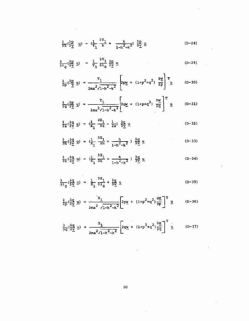
Page 86
k U) = l k a u (D-28)-1 1-h2-k )
a L( ) 1 1 22 u (D-29)ax 0 v - Y1 a0 av-
~ ( u) = 1pw + (l+p 2 + 2 ) u (D-30)
2ma /1-h -k 2
a(2 u) = qw_ + (+p+q 2 ) u (D-31)a9 2 -2 1 2
2ma /l-h -k
a ( u) ax i - (D-32)v- x1 a u
( ) = X 1 + h+ ) (D-33)- 1 1-h-k --
( ) 1 ~ + k a u (D-34)1 1-h -k -
a-o2 u) 1 ax= + _u (D-35)a0x 1 0
u) = 2 2 - 2PW + (1+p2 2 ) +q (D-36)
2ma 11-h 2 -k 2 -
Sm) = - fl 2 + (l+p2+q2)] u (D-37)
2ma /1-h 2_k 90
90
Page 87
a 1 ax1 1 a 3 mat a r + 2) + a sin F(hB - sin F)
aah a h r- r
+ cos2] (D-38)
2X1 h23 32h32 a[-cos F(B + 1 - + (k sin F) - h cos F) 1-."
a a 2X+ h53 2Xl- p cos F - cos F 3F3+ B 3 h
2 a 2X 1
- [ cos F(1 + k sin F - h cos F) + a sin F 2
r arah
(D-39)
2X1 h283 a2X kB 3 2X1- a sin F (B + - ) + sin F +F3h + ao2h
akah r Mh 1-R 9 ah
2 2 x1S sin (1 + k sin F - h cos F - a cos (D-4rh
a2X 2X 2 a2X1 (D-40)
ax0ah = h + - (l+k sin F - h cos F) -ar-ah (D-41)
a2 (1 - h 3 + a sin F)(hp - sin F)
aFah a ( + r
+ cos2F (D-42)r
2 X1 h28 3 (3-28) a= a sin F - h cos F)(1 + (3-2) h cos F[aj(k sin r
(D-43)
a2X1 a2
ara - cos F (hB - sin F) (D-44)r
91
Page 88
aX1 1 1 3 mat r hkB3 a2 1 3 mat -) hk3 cos F (2 sinF - h)]aak a ak 2 r a 1- r
(D-45)
1= (D-46)
2 2aX1 ah83 a. 21
-2- 1 ah- (2k sin F - h cos F) + S sin F a x
ak
k83 32X 1 2+ 17 + r sin F(1 + k sin F - h cos F)
2
a cos F- (D-47)
a2x a2x 22X a 2X a2 k 2X
0 ar Fak + - (1 +k sin F - h cos F) k (D-48)
2X 3Xak1 F r hk8r (D-48)
2X 2l( a h sin F (sin F - h-) (D-51)
1 1 1 3 mat r kh3 aah - a 1-h r ) 1-8 r
(D-52)
92
Page 89
82Y 3 a ao Yh1 ak~(k sin F - 2h cos F) - cos F
Dh2 1-a r DFah
h3 32Y 2+ h6 1-_ a2Yp cos F(1 + k sin F - h cos F)1- apah r
+ a sin F -r (D-53)
21 hB3 a1k2 h = a -i2 (2k sin F - h cos F) + - pcos F2 2.B r
a2 k23 2Y 2.a2+ a sin F + + sin F(1 + k sin F
r aFah 1-W h ah
- h cos F) - a cos F rh (D-54)
I 2Y
2Y1 a 32 Y 2 2Y1= + - (1 + k sin F - h cos F) (D-55)
ax 0h r rr Dr2h
y1 a - 1) kh sin F (k - 2cos F) (D-56)Fh- a( -a r I
82h - a (k sin F - h cos F) kh 2(3-2) +a k cos Fah ( 2 r (D-57)
S2Y 1 2rh = - 2 cos F(ka - cos F) (D-58)
r
93
Page 90
a2 Y 1 1 3 mat r k2a31a5k a k 2 r 1)(8 + -8
+ a cos F (cos F - kB) a sin2F (D-59)r r
1 1 (D-60)ahlk =aa
2 1 k2 3 32kBk28a sin F (0 + /-) + (h cos F - k sin F)( )
a iy a2Y k3 2Y1sin F + asin F 3Fah 1-B -
a2 sin F(1 + k sin F - h cos F)- a cos F] 2r ar3k
(D-61)
2Y1 a a2Y1 2 2Y03X k r -F -- (1 + k sin F - h cos F) -- (D-62)
2Y 23
F = a - 1)(8 + -a ) + a cos F (cos F - k8)
a sin 2 ] (D-63)r
2I k22 (3-28) aayk a (h cosF - k sin F)( 1+ (1)2 (3-2 ) - k sin F
(D-64)
94
Page 91
a2Y 2
S- sin F (cos F - kB) (D-65)r
f 2 [ q g + w] (D-66)
DP l+p2 +q2
f 2 (D-67)
1q l+p +q2
S= 2 q f (D-68)ap 2 2 f
1+p +q
S= 2 f - w] (D-69)
q l1+p2 +q2
w 2 f (D-70)
p 2 2Sl+p +q2 -
w 2 (D-71)
q 1+p +q
T_Xf (D-72)
a a f
Tax r
_ =f (D-73)
0 95
95
Page 92
- g (D-74)
1 ~-
- g (D-75)
Tf (D-76)
aa aa
f (D-77)
avTS g (D-78)3a ia 9
av T
X= X g (D-79)
96
Page 93
REFERENCES
1. Athans, M., "The Role and Use of the Stochastic Linear-Quadra-
tic -Gaussian Problem in Control System Design," IEEE Transaction on
Automatic Control, Vol. AC-16, No. 6, 1971.
2. Battin, R.H., Astronautical Guidance, McGraw-Hill, New York,
1964.
3. Bryson, A.E.,Jr., and Ho, Y.C., Applied Optimal Control, Waltham,
Mass., Blaisdell, 1969.
4. Cefola, P.J., "Equinoctial Orbit Elements - Application to Arti-
ficial Satellite Orbits," Computer Science Corporation, Silver Spring,
Maryland.
5. Kalman, R.E., and Bucy, R.S., "New Results in Linear Filtering
and Prediction Theory," Trans. A SME, Ser. D.J. Basic Eng. 83, 1961.
6. Meier, L. III, Lawson, R.E., and Tether, A.J., "Dynamic Program-
ming for Stochastic Control of Discrete Systems," IEEE Transactions
on Automatic Control, Vol. AC-16, No. 6, Dec. 1971.
7. Jazwinski, A.H., Stochastic Processes and Filtering Theory,
Academic Press, New York, 1970.
8. Shepperd, S.W., "Low Thrust Optimal Guidance for Geocentric
Missions," Sc.M. Thesis, M.I.T., 1972.
9. Speyer, J.L., Deyst, J.J., and Jacobson, D.H., "Optimization of
Stochastic Linear Systems with Additive Measurement and Process Noise
Using Exponential Performance Criteria," to be appearing.
97
Page 94
10. Wong, E., Stochastic Processes in Information and Dynamical
Systems, McGraw-Hill, New York, 1971.
11. Wonham, W.M., "On the Separation Theorm of Stochastic Control,"
SIAM J. Control, Vol. 6, No. 2, 1968.
98