TVE 14 041 juni

Examensarbete 15 hpJuni 2014

Force Measurements on Permanent Magnets and Demagnetization Effects of Assembling Halbach Arrays

Andreas ÖstmanMax Ivedal

Teknisk- naturvetenskaplig fakultet UTH-enheten Besöksadress: Ångströmlaboratoriet Lägerhyddsvägen 1 Hus 4, Plan 0 Postadress: Box 536 751 21 Uppsala Telefon: 018 – 471 30 03 Telefax: 018 – 471 30 00 Hemsida: http://www.teknat.uu.se/student

Abstract

Force Measurements on Permanent Magnets andDemagnetization Effects of Assembling HalbachArraysAndreas Östman and Max Ivedal

This project has studied axial forces for the attractiveand repulsive cases between paris of NdFeB permanentmagnets at different distances. Demagnitization whenassembling Halbach arrays has also been studied. Thepractical measurements of the magnetic forcescorresponded to the performed simulations with someexceptions. Those exceptions were due tomeasurement errors. Permanent demagnitization wasnot noticed when assembling the Halbach arrays norwhen pushing two repulsive magnets together in theforce measurements.

ISSN: 1401-5757, TVE 14 041 juniExaminator: Martin SjödinÄmnesgranskare: Henrik OlssonHandledare: J. José Perez Loya and Stefan Sjökvist

Contents

1 Introduction 21.1 Background . . . . . . . . . . . . . . . . . . . . . . . . . . . . . . . . . . 21.2 Motivation . . . . . . . . . . . . . . . . . . . . . . . . . . . . . . . . . . . 21.3 Aim of the project . . . . . . . . . . . . . . . . . . . . . . . . . . . . . . 2

2 Theory 32.1 Permanent magnets . . . . . . . . . . . . . . . . . . . . . . . . . . . . . . 32.2 Halbach Arrays . . . . . . . . . . . . . . . . . . . . . . . . . . . . . . . . 42.3 Hysteresis curves . . . . . . . . . . . . . . . . . . . . . . . . . . . . . . . 52.4 Calculations . . . . . . . . . . . . . . . . . . . . . . . . . . . . . . . . . . 6

2.4.1 Calculations in MATLAB . . . . . . . . . . . . . . . . . . . . . . 7

3 Simulations 83.1 Simulations using FEM . . . . . . . . . . . . . . . . . . . . . . . . . . . . 83.2 2D-force simulations between two cylindrical magnets . . . . . . . . . . . 10

4 Experiment preparations 104.1 Holder design . . . . . . . . . . . . . . . . . . . . . . . . . . . . . . . . . 11

5 Method 155.1 Calibration of load cell . . . . . . . . . . . . . . . . . . . . . . . . . . . . 155.2 Force measurements . . . . . . . . . . . . . . . . . . . . . . . . . . . . . 16

5.2.1 Setup . . . . . . . . . . . . . . . . . . . . . . . . . . . . . . . . . 165.2.2 Procedure . . . . . . . . . . . . . . . . . . . . . . . . . . . . . . . 17

5.3 Assembly of Halbach Arrays . . . . . . . . . . . . . . . . . . . . . . . . . 18

6 Results 196.1 Calibration of load cell . . . . . . . . . . . . . . . . . . . . . . . . . . . . 196.2 Force Measurements . . . . . . . . . . . . . . . . . . . . . . . . . . . . . 206.3 Demagnetization in force measurements (repulsive case) . . . . . . . . . . 236.4 Demagnetization when assembling Halbach arrays . . . . . . . . . . . . . 236.5 Error calculations . . . . . . . . . . . . . . . . . . . . . . . . . . . . . . . 24

6.5.1 Instrument errors . . . . . . . . . . . . . . . . . . . . . . . . . . . 246.5.2 Calibration errors . . . . . . . . . . . . . . . . . . . . . . . . . . . 246.5.3 Force measurement errors . . . . . . . . . . . . . . . . . . . . . . 24

7 Discussion 257.1 Causes of errors . . . . . . . . . . . . . . . . . . . . . . . . . . . . . . . . 257.2 Improvements . . . . . . . . . . . . . . . . . . . . . . . . . . . . . . . . . 25

8 Conclusions 25

1

1 Introduction

1.1 Background

Permanent magnets have got many application areas in society, ranging from small fridgemagnets to smart mobile phones. In order to develop new technologies involving magnetsand to improve existing ones, it is necessary to thoroughly understand the physics behindthem.

1.2 Motivation

This project was performed at the Division of Electricity at Uppsala University andstudied how forces between two permanent magnets vary with the distance between themagnets. An additional assessment was to investigate whether demagnetization occurswhen two repulsive magnets approach one another.

Demagnetization in different permanent magnet applications can cause undesirableeffects. Using models for demagnetization can help engineers to predict problems withtheir design.1

1.3 Aim of the project

The goal of this project was to measure the forces that arise when permanent magnetsare approaching each other. Since a magnetic field sufficiently strong acting on a magnetwill cause it to become partly demagnetized, it is an important aspect to know exactlyhow close the magnets can be pushed without causing changes to its magnetic abilities.

Two types of setups were studied. These included Halbach arrays and pairs of cylin-drical magnets. In the case of the Halbach array setups the main object to assess waswhether demagnetization occurs when a Halbach array is assembled. All magnets usedwere of the type Neodymium Iron Bromide (NdFeB). The dimensions of the cylindricaland cube magnets can be seen in table 1 and 2 respectively

Table 1: Dimensions and types of cylindrical magnets studied.

Magnet type Diameter [mm] Height [mm]N45 4 3N45 4 2N42 20 10

Table 2: Dimensions and the type of cuboidal magnet studied.

Magnet type Side length [mm]N45 3

1Ruoho S. “Modeling demagnetization of sintered NdFeB magnet materials in time-discretized finiteelement analysis”. Helsinki: Aalto print. 2011

2

2 Theory

2.1 Permanent magnets

Permanent magnets are objects that produces magnetic fields. The magnetic fields arenot visible for the human eye but the impact of these fields can be clearly seen in manyeveryday situations. The source of magnetism is partly a result of unfilled electron shellsof atoms as well as due to the rotation of the electrons around the nucleus. Unfilledatomic shells gives rise to a net magnetic field because of the electrons spin. A filledatomic shell would have an equal amount of electrons with spin up and down, resultingin no net magnetic field . An unfilled shell on the other hand, would result in the smallmagnetic contributions from the orbiting electrons not canceling out and thereby giverise to a net magnetic field of the atom.2

Looking at a larger scale, a material will align its atoms and chunks of atoms (domains)in a different manner, namely the one that requires the lowest energy. Since each atomwith an unfilled shell gives rise to a small magnetic field, the atoms themselves couldinformally be considered as small bar magnets. When the small ”magnets” are alignedin an non-ordered fashion the resulting field will be very weak but when they are alignedin an ordered fashion the resulting field will be strong, see figure 1 and 2.

Figure 1: Several atoms (left) illustrated as small bar magnets. When all of these “mag-nets” are aligned in the same direction the material will produce a net magnetic field andas indicated by the arrow, behave as a permanent magnet.

2Jindal UC. Material Science and Metallurgy. Pearson Education India; 2013

3

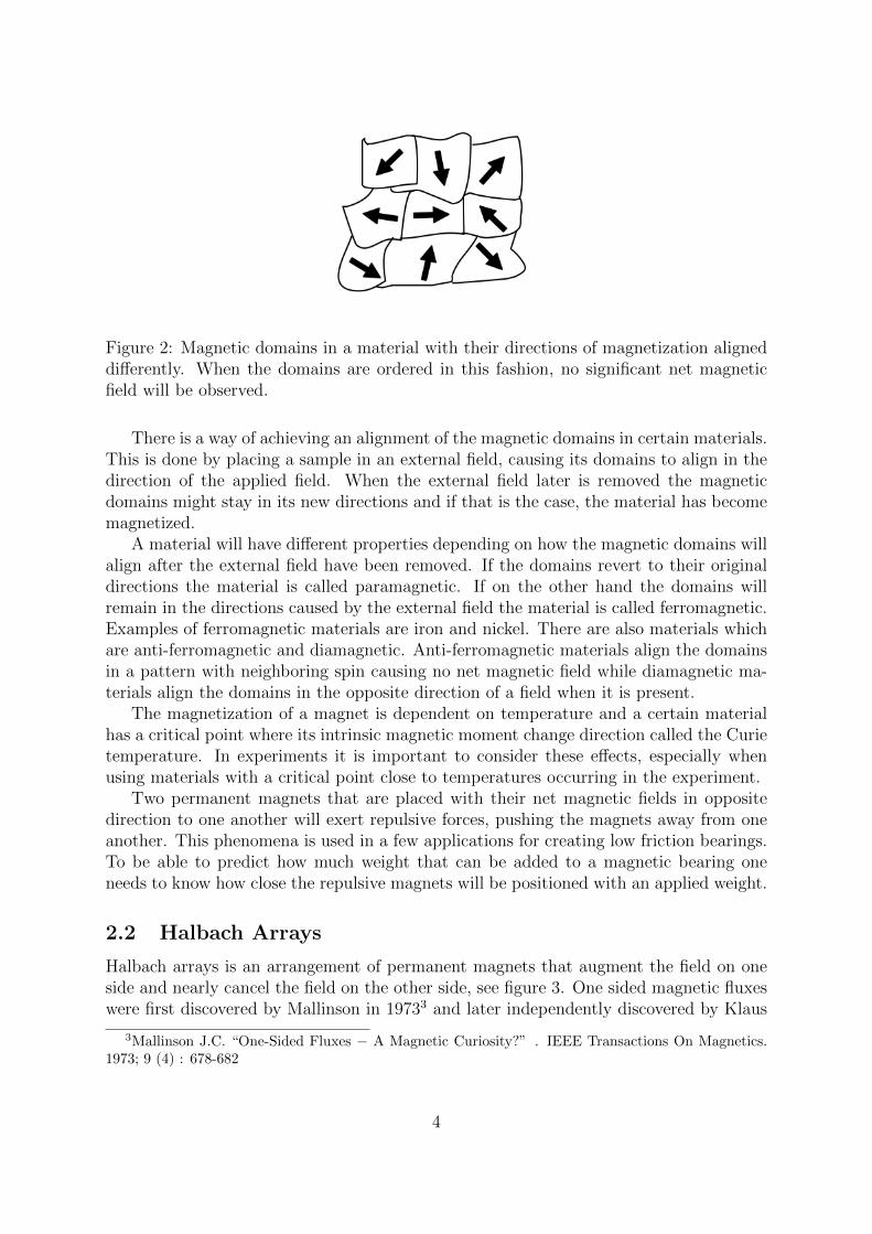
Figure 2: Magnetic domains in a material with their directions of magnetization aligneddifferently. When the domains are ordered in this fashion, no significant net magneticfield will be observed.

There is a way of achieving an alignment of the magnetic domains in certain materials.This is done by placing a sample in an external field, causing its domains to align in thedirection of the applied field. When the external field later is removed the magneticdomains might stay in its new directions and if that is the case, the material has becomemagnetized.

A material will have different properties depending on how the magnetic domains willalign after the external field have been removed. If the domains revert to their originaldirections the material is called paramagnetic. If on the other hand the domains willremain in the directions caused by the external field the material is called ferromagnetic.Examples of ferromagnetic materials are iron and nickel. There are also materials whichare anti-ferromagnetic and diamagnetic. Anti-ferromagnetic materials align the domainsin a pattern with neighboring spin causing no net magnetic field while diamagnetic ma-terials align the domains in the opposite direction of a field when it is present.

The magnetization of a magnet is dependent on temperature and a certain materialhas a critical point where its intrinsic magnetic moment change direction called the Curietemperature. In experiments it is important to consider these effects, especially whenusing materials with a critical point close to temperatures occurring in the experiment.

Two permanent magnets that are placed with their net magnetic fields in oppositedirection to one another will exert repulsive forces, pushing the magnets away from oneanother. This phenomena is used in a few applications for creating low friction bearings.To be able to predict how much weight that can be added to a magnetic bearing oneneeds to know how close the repulsive magnets will be positioned with an applied weight.

2.2 Halbach Arrays

Halbach arrays is an arrangement of permanent magnets that augment the field on oneside and nearly cancel the field on the other side, see figure 3. One sided magnetic fluxeswere first discovered by Mallinson in 19733 and later independently discovered by Klaus

3Mallinson J.C. “One-Sided Fluxes − A Magnetic Curiosity?” . IEEE Transactions On Magnetics.1973; 9 (4) : 678-682

4

Halbach 4. At the time Mallinson described what he called “A magnetic curiosity”, notmany possible applications were considered. When Halbach later made the discovery hesaw applications in particle accelerators among other things. The effect of producing astrong one sided magnetic field makes Halbach arrays useful in some applications, forexample magnetic levitating trains.

Figure 3: An example of a Halbach array with the net magnetic field pointing upwards.The field on the other side of the array nearly cancels out.

2.3 Hysteresis curves

To visualize the behavior of permanent magnets when exerted to an external field socalled hysteresis curves are used. These curves, often referred to as BH-curves, showshow the flux density B of a magnet varies with the applied external field H. There aretwo curves that are studied on the hysteresis plots. These are the normal curve andthe intrinsic curve. The intrinsic curve shows the same data as the normal curve, plusan additional term of M, the magnetization of the magnet itself. The magnets alwaysoperate on the normal line, so this is the line to study for design purposes. The hysteresiscurves of the magnets used in the experiments are shown in figure 4 and 5.

4Rennie G. Magnetically levitated train takes flight [Internet]. [Place unknown] : [U.S DepartmentOf Energy Research News]; [Date unknown] [2004; cited 2014-05-23]. Available from: http://www.

eurekalert.org/features/doe/2004-11/ddoe-mlt111104.php

5

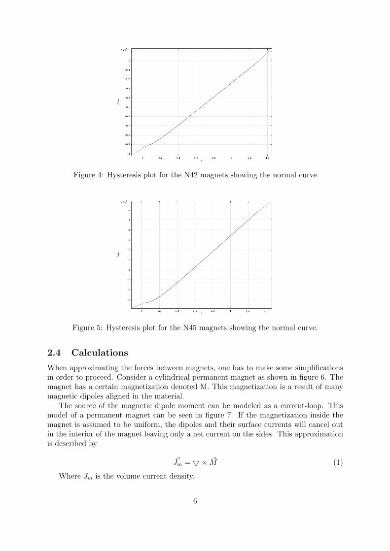
Figure 4: Hysteresis plot for the N42 magnets showing the normal curve

Figure 5: Hysteresis plot for the N45 magnets showing the normal curve.

2.4 Calculations

When approximating the forces between magnets, one has to make some simplificationsin order to proceed. Consider a cylindrical permanent magnet as shown in figure 6. Themagnet has a certain magnetization denoted M. This magnetization is a result of manymagnetic dipoles aligned in the material.

The source of the magnetic dipole moment can be modeled as a current-loop. Thismodel of a permanent magnet can be seen in figure 7. If the magnetization inside themagnet is assumed to be uniform, the dipoles and their surface currents will cancel outin the interior of the magnet leaving only a net current on the sides. This approximationis described by

~Jm = 5× ~M (1)

Where Jm is the volume current density.

6

It can be shown that eq. 1 can be simplified to only account for currents on thesurface of the magnet and the expression then becomes

~Jms = ~M × ~an (2)

where ~an is the normal vector directed outwards from the surface of the magnetas shown in figure 7. The model derived for the magnet is basically the same as themodels for a thin solenoid with a determined height. Because of this, force expressionsfor solenoids can be used to calculate the axial forces between permanent magnets.

Figure 6: A sample of a magnet type N42 with 20 mm diameter and 10 mm height usedin the experiments

Figure 7: The model of an ideal permanent magnet. The arrow pointing from the sideof the magnet corresponds to the direction of the normal vector on that side. The circlesinside the rectangular area shows the magnetic dipoles and the arrows on these circlesshow the direction of the current of each dipole

2.4.1 Calculations in MATLAB

To compare with measured results, the model of a permanent magnet previously derivedwas used and forces were calculated with MATLAB using the expression for thin solenoids

7

derived by Iwaza 5. These calculations are only valid for the attractive forces betweenmagnets.

3 Simulations

3.1 Simulations using FEM

Simulations were performed in order to verify the measured results. This was done forboth attractive and repulsive cases using Comsol.

In order to simulate the setups in Comsol some assumptions had to be made. Thecomplete geometry with the different domains can be seen in figure 8

• Due to symmetry only a slice of the setup needed to be simulated in the case of thecylindrical magnets.

• The surroundings of the magnets were assumed to be air,

• The boundaries of the air-domain were assumed to be perfect magnetic conductorsin the case of attractive magnets. This means that the field lines penetrate theboundary perpendicular and all of the field is preserved throughout the boundary.When simulating the repulsive case the boundaries were set as magnetic insulators.It means that no magnetic field can traverse the boundary and this correspondswell with two repulsive magnets approaching each other. See figure 9 and 10 fordetails.

• Outside the surrounding air-layer an infinite element domain was selected. Thismeans COMSOL approximates an infinite surrounding, see figure 8.

Figure 8: The geometry when simulating forces between cylindrical magnets in Comsol.Domain 1 corresponds to the surrounding air, domain 2 is the magnet and domain 3 isthe infinite element domain

5Iwaza Y. Case Studies in Superconducting Magnets: Design and Operational Issues. Second edition.New York, USA: Springer Science+Business Media; 2009. p.88-89

8

Figure 9: The selected boundary (2) and (9) shows where the perfect magnetic conductorboundary condition was set

Figure 10: The selected boundaries shows were the magnetic insulation boundary condi-tions were set

The magnets in these simulations were set to have a relative permeability that variesdepending on the field they were exerted to. This data was obtained from the magnetmanufacturers data sheets of the BH-curves and were included in the simulations.6 TheBH-curves were included in the simulations by setting the relative permeability to vary

6Neodymium-Iron-Boron Magnets: Summary Listing. Arnold Magnetic Technologies Corp. Availablefrom: http://www.arnoldmagnetics.com/Neodymium_Literature.aspx

9

as a function of the remanent field and the external field. That way the assumption ofhaving an ideal magnet is not needed to be done.

3.2 2D-force simulations between two cylindrical magnets

The force simulations on two cylindrical magnets were made for attractive and repulsivecases with a 2D axissymetrically configuration. This means there is an axis which servesas an axis of symmetry for the simulation. In that way cylindrically shaped geometriescan be simulated. The desired output of the simulations were the forces two cylindricalmagnets exerted on each other depending on the distance between them. To achieve thisthe distance was varied by using a parametric sweep in COMSOL. Setting the bound-ary conditions along with initial conditions giving a contribution in the axissymmetricaldirection, an approximation of the forces were made. Simulations were made for thedifferent dimensions of cylinders shown in table 1. An example of a simulation made forthe larger cylinders can be seen in figure 11

Figure 11: Example of a repulsive simulation showing the magnetic field for the cylinderswith 20 mm diameter and 10 mm height made in Comsol. The white part of the plotshows singularities in the simulation that do not influence the result of the simulation.

4 Experiment preparations

In order to make practical experiments it was necessary to design a setup for the forcemeasurements. One magnet was to be attached into a holder and the holder was connected

10

to the load cell through a screw. The configuration could be moved vertically towards thesecond magnet, and for different positions, the force it exerted on the other magnet wasmeasured. The holders were designed in Solidworks and later printed with a 3D-printer.

4.1 Holder design

It was necessary to design a holder that was able to keep one magnet fixed while exerted toa force from the opposite magnet. Since force measurements was to be done on magnetsof different sizes it was necessary to make a design that accounted for this.

The initial design consisted of four different holders, two magnet holders in whichthe magnets would be glued , one main holder in which this magnet holder would beattached and one lower holder in which the second magnet holder would be attached.The main holder was to be assembled from three parts; a larger frame to which twoarms were attached. These two arms would then be connected by screws to one of themagnet holders. The lower holder was attached to a larger aluminium frame to ensurethat there were no objects close enough to influence magnetic fields of the magnets duringthe measurement.

In the configuration described the magnet holders would expose one of its circularsurfaces to the opposing magnet. The initial design attempt can be seen in figures 12 -14. After examining the first design another design was however chosen. The horizontalscrews were changed for vertically placed ones and the frame holding the magnet holderwas constructed as one solid piece instead of being assembled from several pieces. Non-magnetic screws with a diameter of 8 mm were used for assembling the final design. Thefinal design can be seen in figure 15 and 16. Note that the pieces are not shown in theorientation of the final assembly to show the details of each holder. The design of thelower holder is the same is in the initial attempt. An additional holder for the hall probewas designed to measure the magnetic field.

The final design had a more stable construction as the upper magnet holder wasscrewed onto the main holder in the vertical direction. A vertical setup would avoidtorque and thereby ensure that emerging forces would not alter the horizontal positionof the upper magnet holder. This design allowed more powerful screws that kept thecomponents in place when exerted to magnetic forces.

11

Figure 12: One of the arms of the first design that was to be attached to the main holderand the small holder

Figure 13: The main holder of the first design

12

Figure 14: The small holder of the first design attempt

Figure 15: The small magnet holder of the final design

13

Figure 16: The lower holder of the initial and final design

Figure 17: The main holder of the final design

14

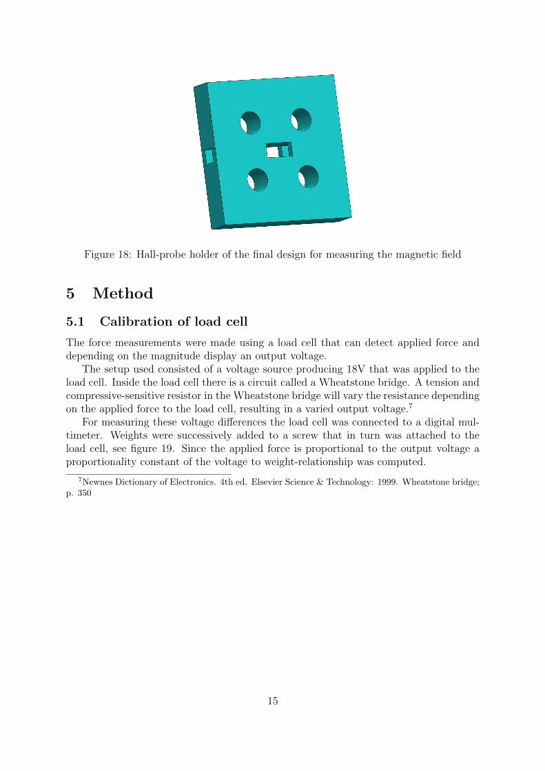
Figure 18: Hall-probe holder of the final design for measuring the magnetic field

5 Method

5.1 Calibration of load cell

The force measurements were made using a load cell that can detect applied force anddepending on the magnitude display an output voltage.

The setup used consisted of a voltage source producing 18V that was applied to theload cell. Inside the load cell there is a circuit called a Wheatstone bridge. A tension andcompressive-sensitive resistor in the Wheatstone bridge will vary the resistance dependingon the applied force to the load cell, resulting in a varied output voltage.7

For measuring these voltage differences the load cell was connected to a digital mul-timeter. Weights were successively added to a screw that in turn was attached to theload cell, see figure 19. Since the applied force is proportional to the output voltage aproportionality constant of the voltage to weight-relationship was computed.

7Newnes Dictionary of Electronics. 4th ed. Elsevier Science & Technology: 1999. Wheatstone bridge;p. 350

15

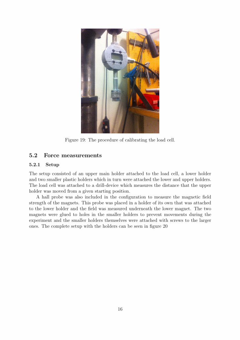
Figure 19: The procedure of calibrating the load cell.

5.2 Force measurements

5.2.1 Setup

The setup consisted of an upper main holder attached to the load cell, a lower holderand two smaller plastic holders which in turn were attached the lower and upper holders.The load cell was attached to a drill-device which measures the distance that the upperholder was moved from a given starting position.

A hall probe was also included in the configuration to measure the magnetic fieldstrength of the magnets. This probe was placed in a holder of its own that was attachedto the lower holder and the field was measured underneath the lower magnet. The twomagnets were glued to holes in the smaller holders to prevent movements during theexperiment and the smaller holders themselves were attached with screws to the largerones. The complete setup with the holders can be seen in figure 20

16

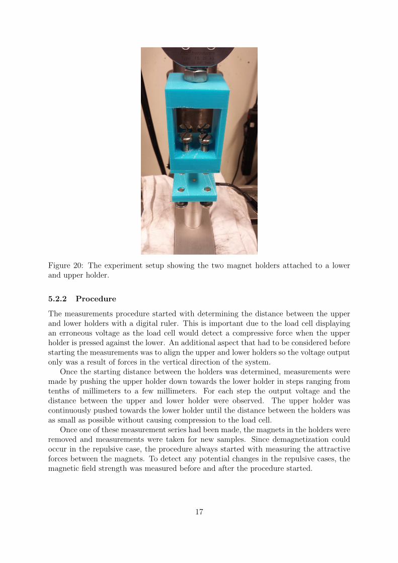
Figure 20: The experiment setup showing the two magnet holders attached to a lowerand upper holder.

5.2.2 Procedure

The measurements procedure started with determining the distance between the upperand lower holders with a digital ruler. This is important due to the load cell displayingan erroneous voltage as the load cell would detect a compressive force when the upperholder is pressed against the lower. An additional aspect that had to be considered beforestarting the measurements was to align the upper and lower holders so the voltage outputonly was a result of forces in the vertical direction of the system.

Once the starting distance between the holders was determined, measurements weremade by pushing the upper holder down towards the lower holder in steps ranging fromtenths of millimeters to a few millimeters. For each step the output voltage and thedistance between the upper and lower holder were observed. The upper holder wascontinuously pushed towards the lower holder until the distance between the holders wasas small as possible without causing compression to the load cell.

Once one of these measurement series had been made, the magnets in the holders wereremoved and measurements were taken for new samples. Since demagnetization couldoccur in the repulsive case, the procedure always started with measuring the attractiveforces between the magnets. To detect any potential changes in the repulsive cases, themagnetic field strength was measured before and after the procedure started.

17

5.3 Assembly of Halbach Arrays

To investigate whether demagnetization occurs when constructing a Halbach array ofcuboidal magnets, plastic holders were printed for the assembly. Two different types ofholders were designed, one cylindrical type and one rectangular type. In the cylindricaltype the magnets were pushed one by one into the holder, see figure 21 for the design.The direction of magnetization of each magnet inside the cylindrical Halbach holder canbe seen in figure 22. In the rectangular design a Halbach was assembled by first gluing theside-magnets onto the holder and then pushing the middle magnet in between and keepingit in position for approximately one minute before removing it. The middle magnet wasassembled with the direction of magnetization in two different ways, see figure 23 - 26.

To keep track of the direction of the magnetic fields of the magnets during the con-struction of a Halbach array, one of the sides of the magnet was colored. When assemblinga Halbach in the cylindrical holder one of the sides of the cylinder was also colored tokeep track of which side was up and down and to produce a net magnetic field in thedesired direction. In both experiments the magnetic field was measured before and afterthe assembly to detect potential changes.

Figure 21: Design of the cylindrical Halbach array holder

Figure 22: Direction of positive fields for the assembly in the cylindrical Halbach holder.The net field is directed upwards.

18

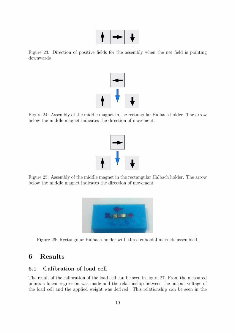
Figure 23: Direction of positive fields for the assembly when the net field is pointingdownwards

Figure 24: Assembly of the middle magnet in the rectangular Halbach holder. The arrowbelow the middle magnet indicates the direction of movement.

Figure 25: Assembly of the middle magnet in the rectangular Halbach holder. The arrowbelow the middle magnet indicates the direction of movement.

Figure 26: Rectangular Halbach holder with three cuboidal magnets assembled.

6 Results

6.1 Calibration of load cell

The result of the calibration of the load cell can be seen in figure 27. From the measuredpoints a linear regression was made and the relationship between the output voltage ofthe load cell and the applied weight was derived. This relationship can be seen in the

19

equation shown in the plot. Since the behavior of the load cell was known to be linear thefew measurement points that were taken serves as sufficient data for reliably determiningthe voltage-to-weight relationship.

Figure 27: Result of calibrating the load cell

6.2 Force Measurements

All of the measured forces for the different cylindrical magnets can be seen in figure 28 -33. For the attractive cases the analytical calculations made in MATLAB is included inthe plots.

Figure 28: Experiment, simulation and analytical comparison for the attractive case. Thecylindrical magnets were of type N45 and had a diameter of 4 mm and height of 2 mm

20

Figure 29: Experiment and simulation comparison for the repulsive case. The cylindricalmagnets were of type N45 and had a diameter of 4 mm and height of 2 mm

Figure 30: Experiment, simulation and analytical comparison for the attractive case. Thecylindrical magnets were of type N45 and had a diameter of 4 mm and height of 3 mm

21

Figure 31: Experiment and simulation comparison for the repulsive case. The cylindricalmagnets were of type N45 and had a diameter of 4 mm and height of 3 mm

Figure 32: Experiment, simulation and analytical comparison for the attractive case. Thecylindrical magnets were of type N42 and had a diameter of 20 mm and height of 10 mm

22

Figure 33: Experiment and simulation comparison for the repulsive case. The cylindricalmagnets were of type N42 and had a diameter of 20 mm and height of 10 mm

6.3 Demagnetization in force measurements (repulsive case)

Demagnetization effects while performing the different force measurements were studied.The magnetic field strength of each magnet was measured before and after the experiment.There were no signs of permanent demagnetization in any of the experiments.

6.4 Demagnetization when assembling Halbach arrays

The initial and final magnitude of the magnetic field for each of the magnets before beingassembled in the cylindrical Halbach holder design is shown in table 3. The direction ofthe magnets were as shown in figure 22.

The results of the assembly in the rectangular Halbach holder configuration with theresulting magnetic field upwards and downwards as shown in figure 24 and 25 can be seenin table 4 and 5 respectively.

As can be seen there is no significant difference in the magnitude before and after theassemblies. The reason some of the fields measured after the assembly are larger thanbefore is most likely due to errors and inaccuracies using the measurement equipment.

Table 3: Field measurements on cuboidal magnets before and after assembly in cylindricalHalbach holder

Initial field strength Final field strength Positive orientation of magnet0.369± 0.05 T 0.375± 0.05 T ↑0.387± 0.05 T 0.389± 0.05 T ←0.389± 0.05 T 0.383± 0.05 T ↓

23

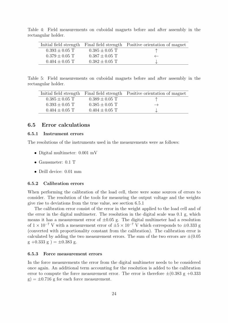
Table 4: Field measurements on cuboidal magnets before and after assembly in therectangular holder.

Initial field strength Final field strength Positive orientation of magnet0.393± 0.05 T 0.385± 0.05 T ↑0.379± 0.05 T 0.387± 0.05 T ←0.404± 0.05 T 0.382± 0.05 T ↓

Table 5: Field measurements on cuboidal magnets before and after assembly in therectangular holder.

Initial field strength Final field strength Positive orientation of magnet0.385± 0.05 T 0.389± 0.05 T ↑0.393± 0.05 T 0.385± 0.05 T →0.404± 0.05 T 0.404± 0.05 T ↓

6.5 Error calculations

6.5.1 Instrument errors

The resolutions of the instruments used in the measurements were as follows:

• Digital multimeter: 0.001 mV

• Gaussmeter: 0.1 T

• Drill device: 0.01 mm

6.5.2 Calibration errors

When performing the calibration of the load cell, there were some sources of errors toconsider. The resolution of the tools for measuring the output voltage and the weightsgive rise to deviations from the true value, see section 6.5.1

The calibration error consist of the error in the weight applied to the load cell and ofthe error in the digital multimeter. The resolution in the digital scale was 0.1 g, whichmeans it has a measurement error of ±0.05 g. The digital multimeter had a resolutionof 1× 10−7 V with a measurement error of ±5× 10−7 V which corresponds to ±0.333 g(converted with proportionality constant from the calibration). The calibration error iscalculated by adding the two measurement errors. The sum of the two errors are ±(0.05g +0.333 g ) = ±0.383 g.

6.5.3 Force measurement errors

In the force measurements the error from the digital multimeter needs to be consideredonce again. An additional term accounting for the resolution is added to the calibrationerror to compute the force measurement error. The error is therefore ±(0.383 g +0.333g) = ±0.716 g for each force measurement.

24

7 Discussion

7.1 Causes of errors

The fact that the magnets did not become permanently demagnetized was unexpected.The reason for the constant magnitude of magnetization is probably due to the high co-ercivity of the NdFeB-magnets that were used in the experiment. The external magneticfield has to be larger in order to demagnetize the magnets used.

Some of the measured values differ from the simulations and this is due to measure-ment errors. It was difficult to accurately determine the starting distance between thetwo magnets in the holders and if this relative distance is not correct, all of the measuredpoints will be offset from the simulated values with a certain distance.

In the experiments using the 20 mm diameter and 10 mm high cylindrical magnetsthe measured values are close to the simulated ones. The difference that can be seencould be due to an inaccurate BH-curve being used in the simulations.

There are several causes of potential errors that could have arisen in the experiment.It was hard to determine the exact starting distance between the holders. This was animportant aspect to know in order to prevent the upper holder being pushed too far,resulting in the load cell being compressed and displaying an incorrect value.

Another error source was that the plastic holders themselves were not perfectly planar.This made it impossible to push the upper holder towards the lower one until the distancebetween them was close to zero millimeters. If they would have been pushed to a distanceof zero millimeters while being inclined, the upper and lower holder would have touchedand the output voltage would again be erroneous.

As the holders were assembled with screws, a small air-gap did arise in some of theassemblies. Since the screw holes in the holders were not threaded, the holes were exertedto a certain shear stress and a minor displacement occurred. In experiments using thelarge magnets, this stress could also deform the holder itself.

The 3D-printer used was only able to print with an accuracy of 0.14 mm or 0.19 mmdepending on the settings used. This means that in order for the measurements of aprinting to be exact it was necessary for the size of the model to be a multiple of thechosen accuracy.

7.2 Improvements

To reduce the errors more measurements could have been performed. The holes in theexperimental setup could have been threaded to make the assembly more stable. Thiscould also indirectly have solved the issue of an erroneous distance being measured if theholders were assembled without gaps.

More accurate BH-curves could have been used to improve the simulations and get abetter correspondence between measured and simulated values.

8 Conclusions

The initial hypothesis was that a magnet would change its magnetization if exerted toa sufficiently large external field. No signs of permanent demagnetization was observed,

25

not during the force measurements nor when assembling the Halbach arrays.An interesting observation was that immediately after two repulsive magnets had

been pushed together in the force measurements, signs of demagnetization was noticed.This effect was however only temporary and the field strength reverted to its originalmagnitude rapidly.

The experimental results did for the most part of the measurements resemble theanalytical results. Reasons for differences between analytical and experimental is mostprobably due to measurement errors.

26