Abstract It is known that the average of many forecasts about a future event tends to outper-form the individual assessments. With the goal of further improving forecast performance,this paper develops and compares a number of models for calibrating and aggregating fore-casts that exploit the well-known fact that individuals exhibit systematic biases during judg-ment and elicitation. All of the models recalibrate judgments or mean judgments via a two-parameter calibration function, and differ in terms of whether (1) the calibration functionis applied before or after the averaging, (2) averaging is done in probability or log-oddsspace, and (3) individual differences are captured via hierarchical modeling. Of the non-hierarchical models, the one that first recalibrates the individual judgments and then aver-ages them in log-odds is the best relative to simple averaging, with 26.7 % improvementin Brier score and better performance on 86 % of the individual problems. The hierarchicalversion of this model does slightly better in terms of mean Brier score (28.2 %) and slightlyworse in terms of individual problems (85 %).
Keywords Calibration · Aggregation · Forecasting · Systematic distortions · HierarchicalBayesian models · Individual differences · Wisdom of the crowd
Editors: Winter Mason, Jennifer Wortman Vaughan, and Hanna Wallach.
B.M. TurnerStanford University, 450 Serra Mall, Stanford, CA 94305, USA
M. Steyvers (B)University of California, Irvine, CA 92697, USAe-mail: [email protected]
E.C. MerkleUniversity of Missouri, 319 Jesse Hall, Columbia, MO 65211, USA
D.V. BudescuFordham University, 441 East Fordham Road, Bronx, NY 10458, USA
T.S. WallstenUniversity of Maryland, 8082 Baltimore Avenue, College Park, MD 20740, USA
In many situations, experts are asked to provide subjective probability or confidence esti-mates of uncertain events. The estimates can relate to general knowledge questions (e.g.,Which city is furthest North of the equator, Rome or New York?) or to predicting eventoccurrence (e.g., Will political candidate X win the election?). There exists a large body ofwork focused on the use of statistical models for combining these individual subjective prob-ability judgments into a single probability estimate (e.g., Ariely et al. 2000; Clemen 1986;Clemen and Winkler 1986; Cooke 1991; Wallsten et al. 1997). A simple form of aggregation,namely the unweighted linear average, has proven to be effective in many situations (e.g.,Armstrong 2001). Alternatively, the aggregation can be accomplished by taking a weightedaverage of the reported probability estimates, with, for example, weights determined byprevious expert performance (Cooke 1991).
We consider the aggregation of subjective forecasts voluntarily provided by users of awebsite. This is similar in spirit to the machine learning notion of aggregating across weaklearners, as implemented in popular methods such as bagging (Breiman 1996) and boosting(Freund and Schapire 1996). The former method involves fitting a series of weak learners(often classification or regression trees) to bootstrapped samples of the data, with overall pre-dictions obtained by averaging across the weak learners. The latter method involves fitting aseries of weak learners to weighted versions of the original dataset, with overall predictionsobtained by taking an accuracy-weighted average across the weak learners. The aggrega-tion of weak machine learning algorithms differs from the aggregation of human forecastsin that (i) given a domain, the algorithms often exhibit more stable behavior, and (ii) thehumans often contribute only a small number of forecasts. While the ideas of averaging andweighting weak learners definitely translate to the aggregation of human forecasts, specificimplementations must deal with these additional data sparsity and variability problems.
An important consideration for aggregation approaches involving human forecasts is thepresence of systematic biases that might distort the individuals’ subjective probability es-timates. For example, when using probabilities to report confidence in one’s judgment, in-dividuals often report values that are too extreme (e.g., Brenner et al. 1996; Keren 1991;Lichtenstein et al. 1982; Yates 1990). Merkle (2010) estimated and corrected for these sys-tematic biases in psychological data. Further, Shlomi and Wallsten (2010) have shown thatjudges are sensitive to miscalibrated subjective probabilities, and they are able to internallyrecalibrate miscalibrated information from advisors. These findings suggest that we mightimprove forecast aggregation by correcting for forecasters’ systematic biases. In this arti-cle, we construct a series of models that first estimate the bias inherent in judges’ forecasts,then correct and aggregate the forecasts into a single value. The models we investigate dif-fer in both the extent to which they accommodate individual differences and where the biascorrection takes place (see Clemen 1989, for a related discussion of the latter issue).
We first present the general recalibration function used in all the models, and then de-scribe five aggregation models that use the function in different ways. We apply the modelsto data from a recent forecasting study, comparing the models to one another and to the un-weighted average forecast. By investigating a wide variety of model variants, we seek to un-derstand which modeling procedure leads to the most accurate forecasting performance, asmeasured by a cross validation test. Our research centers on three questions. (1) Is it better toaggregate the raw individual judgments and then recalibrate the average; to first recalibratethe individual judgments and then average those values; or to recalibrate the individuals, av-erage those values and then recalibrate that average? (2) Regardless of the answer to the firstquestion, how should the recalibration take place—on the probabilities themselves or fol-lowing some transformation, such as log odds? (3) Does including individual differences in
Mach Learn
these models improve accuracy or does it simply reduce their generalizability to new ques-tions? We investigate each of these questions, draw conclusions about optimal calibrationmethods, and relate these conclusions to possibilities for future methods and applications.
2 Recalibrating subjective probability estimates
A large body of evidence suggests that subjective probability estimates systematically de-viate from objective measures (see Zhang and Maloney 2011, for examples across manyresearch domains). In forecasting situations, the probability of rare events is often overesti-mated while the probability of common events is underestimated. This tendency is relatedto the miscalibration that is often found in psychology research. For example, judges con-sistently overestimate the probability of precipitation (Lichtenstein et al. 1982). Murphyand Winkler (1974) asked judges to first report the probability of precipitation for the nextday. After this initial estimate, judges were provided with information from a computerizedweather prediction system, and were asked to reestimate their probabilities. The manipula-tion showed no effect and both responses demonstrated overestimation of the probability ofprecipitation.
Miscalibration in prediction often carries over to natural or expertise domains, but notalways. Griffin and Tversky (1992) found that when judges were asked about attributes suchas population size of pairs of states, they produced significantly overconfident responses. Inthe prediction task, Murphy and Winkler (1984) showed that professional weather forecast-ers are remarkably well-calibrated, producing nearly perfect probability estimates. However,Christensen-Szalanski and Bushyhead (1981) showed that when physicians were asked toestimate the likelihood of pneumonia in patients, they were grossly overconfident (predict-ing probabilities as extreme as 0.88 when the actual probability was only about 0.14). Thisdifference can be explained by the fact that weather forecasters make large numbers of fore-casts and receive relatively immediate feedback on them, while physicians do not (Wallstenand Budescu 1983; Fryback and Erdman 1979). The forecasting situations that are consid-ered below tend to be more similar to those made by physicians than to those made byweather forecasters.
In other experimental paradigms, Brown and Steyvers (2009) asked judges to both inferand predict stimulus properties in a perceptual task involving four alternatives. Their ex-periment consisted of an “inference” task in which subjects were instructed to choose thealternative that was most likely to have produced a particular stimulus, and a “prediction”task in which judges were asked to choose the alternative that was most likely to producethe next stimulus (i.e., a prediction about a future stimulus). On each trial, one of the fouralternatives produced a stimulus in a manner that induced a strong positive sequential de-pendency. Specifically, the alternative that produced the stimulus on Trial t was more likelythan the others to produce the stimulus on Trial t +1. By using the same stimulus set in boththe inference and prediction tasks, Brown and Steyvers found that 48 of the 63 judges esti-mated a higher probability of a change in the prediction task than they did in the inferencetask, suggesting greater miscalibration in the former than in the latter (see also Wright andWisudha 1982; Wright 1982).
As mentioned earlier, judges who accurately estimate the observed relative frequency ofevents are said to be “calibrated.” That is, if a judge reports a probability of occurrence of p,and the event happens pn out of n times, then the judge is well recalibrated. Calibration canbe assessed both visually and statistically. A common empirical approach involves plottingobserved relative frequencies (y-axis) conditional on judged or subjective probabilities (x-axis). In this approach, the relative frequency of occurrence is computed by binning the
Mach Learn
subjective probabilities and computing the proportion of events that occurred within eachbin. The line of perfect calibration is then y = x, with data falling below (above) the lineimplying overconfidence (underconfidence). These plots can also be reinforced with simplestatistical measures of calibration, often based on decompositions of the Brier score (Arkeset al. 1995; Yates 1982).
An alternative approach involves fitting a function to the (X,Y ) plot that characterizesthe nature and extent of the deviation of the points from the diagonal. The function itself canbe used to “recalibrate” the judged probabilities, while estimates of the function’s parame-ters can be used to compare the extent and nature of miscalibration across judges, groups,or experiments. Many different functions are available, but because of its great flexibilitywe decided to use the Linear in Log Odds (LLO) function. Our use is different from previ-ous decision researchers, however. Whereas they were concerned with decision weights inchoice tasks, our focus is on transforming judged probabilities to render them more accurate.
2.1 The linear in log odds function
The LLO recalibration function has been used extensively as a method for estimatingthe distortion of subjective individual probability estimates from their true experimen-tal probabilities in the context of risky decision (e.g., Birnbaum and McIntosh 1996;Gonzalez and Wu 1999; Tversky and Fox 1995). To derive the functional form, we assumethat the recalibration function c(p) is linear with respect to p on the log odds scale, so that
log
(c(p)
1 − c(p)
)= γ log
(p
1 − p
)+ τ, (1)
where γ and τ are the slope and intercept, respectively. If we solve for c(p) in Eq. (1), weobtain the recalibration function
c(p|γ, δ) = δpγ
δpγ + (1 − p)γ, (2)
where δ = exp(τ ). The slope parameter γ in Eq. (1) corresponds to the curvature of thefunction in Eq. (2) and the intercept parameter τ = log(δ) controls the height above zero.
In analogy to Gonzalez and Wu’s (1999) argument about the weighting function param-eters, the recalibration function provides a convenient functional form with two psycholog-ically interpretable parameters. The first parameter γ in our use of the model correspondsto discriminability, which manifests itself in the functional form by means of curvature. Asγ increases, the form of the calibration function becomes more step-like, indicating thatjudges’ estimates of low and high probability events are insufficiently extreme. The sec-ond parameter δ represents overall response tendency, which is represented as the verticaldistance of the curve from zero. Tendencies for higher estimates yield higher calibrationcurves.
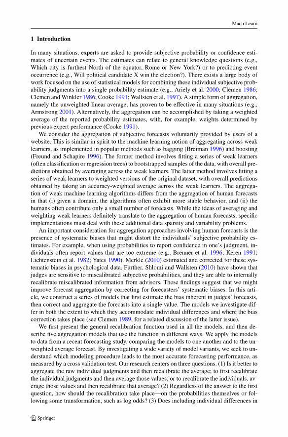
Figure 1 shows various LLO curves as a function of different parameter values. Theleft panel shows how the parameter γ affects the functional form by fixing δ = 0.6 andincrementing γ by 0.1 from γ = 0 to γ = 3. The figure (left panel) shows that as γ isincreased from zero to three, the curves go from being a straight horizontal line to sharplyincreasing on the interval [0.3,0.8]. The right panel shows how δ affects the functional formby fixing γ = 0.2 and incrementing δ by 0.1 from δ = 0 to δ = 3. The figure (right panel)shows that as δ is increased from zero to three, the function increases in height above zero(also known as “elevation”; Gonzalez and Wu 1999).
Mach Learn
Fig. 1 Various LLO curves under different parameter values. The left panel shows how the γ parameteraffects the functional form by fixing δ = 0.6 whereas the right panel shows how δ affects the functional formby fixing γ = 0.2
Figure 1 shows that the function is very flexible and has a number of interesting proper-ties. First, we notice that under the restriction γ = 1 and δ = 1, c(p) = p and no transfor-mation is applied. Second, if δ = 1 the function reduces to another well-known calibrationcurve known as the Karmarkar’s equation (Karmarker 1978). Third, the function must gothrough the points (0,0) and (1,1), which is not always true for some calibration functions.Finally, the function is guaranteed to cross the identity line c(p) = p at exactly one locationp∗ (except when γ = δ = 1) where
p∗ = δ1/(1−γ )
1 + δ1/(1−γ ). (3)
Note that the LLO function does not require that the curve passes through the point(0.5,0.5), nor that it is symmetric. This property implies that the recalibration function isnot a probability function, which by definition must satisfy
c(p) + c(1 − p) = 1.
Functions that do not satisfy this constraint typically provide good fits to empirical data,where the general finding is that judges both overestimate and overweight low-probabilityevents and even more dramatically underestimate and underweight high-probability events(e.g., Camerer and Ho 1994; Tversky and Kahneman 1992; Wu and Gonzalez 1996).
Once a recalibration function has been fit to data for a particular judge, if the sum of therecalibrated values for complementary probabilities is less than one (i.e., c(p)+ c(1 −p) <
1), the judge is said to exhibit subcertainty (Kahneman and Tversky 1979). In our applica-tions, the very flexible form of the LLO recalibration function will be advantageous becausejudges appear to be overly optimistic about the probability of future outcomes (i.e., theytend to provide judgments that are higher than the relative frequency of an event occurring;see Brown and Steyvers 2009).
To estimate the parameters γ and δ in Eq. (2), one can use classic maximum likelihoodmethods. If we let Xj indicate whether the j th event did (Xj = 1) or did not occur (Xj = 0),then the likelihood function is the product
L(γ, δ|X) =∏
i
{c(p|γ, δ)Xj
[1 − c(p|γ, δ)
]1−Xj}, (4)
Mach Learn
where p is a single forecast associated with Event j . To obtain the maximum likelihoodestimates, one uses standard numerical optimization routines to optimize Eq. (4) with respectto γ and δ.
If there are enough data, an alternative to likelihood-based methods are nonparamet-ric estimation techniques (Gonzalez and Wu 1999; Page and Clemen 2012). For example,Gonzalez and Wu proposed a nonparametric estimation algorithm that returns estimates ofthe value and recalibration function in the prospect theory model (Kahneman and Tversky1979), but other recalibrating functional forms can be estimated using this approach. Gonza-lez and Wu found that using the nonparametric approach provided a great deal of flexibilityin fitting the data from a calibration experiment. As another example, Page and Clemenused a localized kernel density estimator (see Silverman 1986) in combination with a clus-tered bootstrap approach (see Härdle 1992) to fit calibration curves to data from a predictionmarket.
One can also employ Bayesian methods to estimate the parameters γ and δ in Eq. (2). Inthe Bayesian framework, one assumes that the parameters, along with the data, are randomquantities (e.g., Gelman et al. 2004). In contrast to classical statistics, inference about theparameters are based on their probability distributions after some data are observed (seeChristensen et al. 2011; Gelman et al. 2004). We rely on Bayesian estimation procedures inthe applications described below.
2.2 Linear in log odds aggregation
For the longitudinal dataset to which we apply the models, some events do not yet haveknown outcomes. We incorporate these missing observations into the vector xj , the result ofthe j th event. When xj = 1, the event did occur—an event we refer to as a resolved event—whereas xj = 0 denotes that the event did not occur—an event we refer to as an unresolvedevent. We let yi,j represent the probability estimate provided by Judge i on Event j . Be-cause Eq. (1) is not defined when p = 0 or p = 1, we must use a correction to judgmentssuch that yi,j = 0 or yi,j = 1 prior to use in the models. Thus, we adjust these boundaryforecasts to 0.001 and 0.999, respectively, prior to fitting any of the models to facilitate adirect evaluation across models.
We generally compare our re-calibration models to the unweighted linear average (some-times called the Unweighted Linear Opinion Pool; ULinOP) of the estimates provided byeach of the judges. Thus, predictions μ̂j for ULinOP are obtained by evaluating
μ̂j = 1
n
(n∑
i=1
yi,j
),
where n is the number of responses obtained on Event j .Despite its simplicity, the ULinOP is a formidable estimate for the probability of future
outcomes in forecasting future events. Some authors have even argued that it is difficult tobeat the ULinOP by more than 20 % (e.g., Armstrong 2001).
The models described below each allow for distortions that yield non-additive probabil-ities. Although we assume that this distortion is a consequence of the functional form inEq. (2), we exploit the recalibration function in a variety of ways. All of the models pre-sented below can be represented in the general form
Model(y) = f(g(y)
), (5)
Mach Learn
Table 1 Model specification as a function of an inner function g(·) and an outer function f (·) according toEq. (5)
Model Inner g(·) Outer f (·)
ULinOP yi (1/n)∑n
i=1 g(yi )
Average then Recalibrate (1/n)∑n
i=1 yi c(g(y)|γ, δ)
Calibrate then Average c(yi |γ, δ) (1/n)∑n
i=1 g(yi )
Calibrate then Average Log Odds log(c(yi |γ,δ)
1−c(yi |γ,δ))
exp[(1/n)∑n
i=1 g(yi )]1+exp[(1/n)
∑ni=1 g(yi )]
where y denotes the set of observed responses, Model(y) represents the predictions of themodel, and g(·) and f (·) are two functions that are either calibration or aggregation func-tions, depending on the model. Table 1 shows the functions g(·) and f (·) for each modelunder consideration. The first type of model we present, Average then Recalibrate, first av-erages all responses for Event j and then calibrates the average to estimate the probability ofan event occurring. The second type of model recalibrates each individual judgment usingthe parameters γ and δ, and then averages these recalibrated judgments to estimate the eventprobability. We explore two variants of this model. In the first version, Calibrate then Aver-age, the averaging is performed directly on the recalibrated judgments. The second variantof this model, Calibrate then Average Log Odds, performs the averaging on the log oddsof the recalibrated judgments. We will show that this second variant leads to much betteraggregation results. Finally, we also examine hierarchical extensions of the recalibrationmodel (not shown in Table 1) that incorporate individual differences into the estimation ofthe parameters γ and δ in Eq. (2).
2.3 Average then recalibrate model
The first model we consider averages the responses for a particular event and then recali-brates the average. One useful way to view this model is as a transformation of the ULinOPdiscussed previously. Instead of taking the group average at face value, the group averageis transformed using Eq. (2). While this type of modeling does not necessarily have clearpsychological interpretability (as individual differences are ignored), it dampens the impactof extreme predictions (i.e., zeros or ones) given by individual judges. In addition, averag-ing the individuals’ biases may produce more stability in the estimation of the calibrationparameters.
Thus, for the j th resolved event, we assumed that
pj = 1
Sj
∑i∈Qj
yi,j ,
μj = c(pj |γ, δ), and
xj ∼ Bernoulli(μj ),
where pj is the average probability elicited by judges for the j th event, xj is the codedknown outcome for the j th event, Qj is the set of judges who responded to the j th event,Sj is the number of judges who responded to the j th event (i.e., Sj = |Qj |), and c(·|γ, δ) is
Mach Learn
governed by Eq. (2). Thus, for the j th event, the likelihood function can be written as
L(γ, δ|xj , yi,j ) =[c
(1
Sj
∑i∈Qj
yi,j
∣∣ γ, δ
)]xj[
1 − c
(1
Sj
∑i∈Qj
yi,j
∣∣ γ, δ
)]1−xj
. (6)
As stated previously, we estimated the models via Bayesian methods that require priordistributions. After some inspection, we settled on mildly informative priors for each of themodel parameters here so that
δ ∼ Γ (1,1) and
γ ∼ Γ (1,1),(7)
where Γ (a, b) denotes the gamma distribution with rate a and shape parameter b. TheΓ (1,1) prior has a mean and standard deviation of 1, and a 95 % credible set of approx-imately (0.025, 3.703). We chose these priors after observing the shape of the calibrationfunction for a representative range of values for γ and δ within this range. We note thata Γ (1,1) prior is equivalent to an exponential prior with rate parameter equal to one (i.e.,Γ (α,1) = Exp(α) for some rate parameter α).
With our fully-specified model, we can now write the joint posterior distribution for γ
and δ as
π(γ, δ|x, y) ∝J∏
j=1
L(γ, δ|xj , yi,j )π(γ )π(δ), (8)
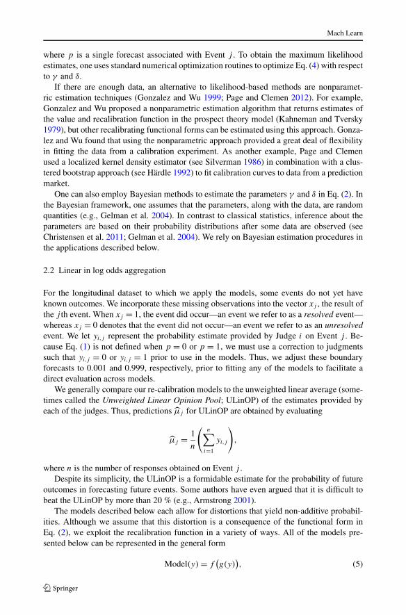
where L(γ, δ|xj , yi,j ) is defined in Eq. (6), and J is the number of resolved events.Figure 2 shows a graphical diagram for this model. These types of diagrams are
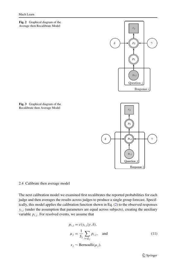
often very useful for illustrating how the parameters in the model (white nodes) areconnected via arrows to the observed data (gray nodes; see Buntine 1994; Lee 2008;Lee and Wagenmakers 2012; Shiffrin et al. 2008). When the variables are discrete-valued,they are shown as square nodes, whereas when the variables are continuous, they are shownas circular nodes. A double bordered variable indicates that the quantity is deterministic,not stochastic. Finally, “plates” show how vector-valued variables are interconnected. Forexample, in Fig. 3, we see that the nodes γ and δ are not on the plate, which indicates thatthese parameters are fixed across events, whereas there are separate μj s for each Event j
ranging from one to J , which are connected to the other nodes on the plate.To elicit a prediction for Event j , the model first calculates the mean of the posterior
distribution for each of the parameters μj , so that
μ̂j = 1
K
(K∑
k=1
μj,k
), (9)
where K is the number of samples drawn from the posterior distribution (see below for moredetails), and μj,k is the kth sample of the posterior corresponding to μj . Once each of theseμj s are obtained, the model returns the estimate
{μ̂j ,1 − μ̂j } (10)
for the probability of the event occurring and the probability of the event not occurring,respectively.
Mach Learn
Fig. 2 Graphical diagram of theAverage then Recalibrate Model
Fig. 3 Graphical diagram of theRecalibrate then Average Model
2.4 Calibrate then average model
The next calibration model we examined first recalibrates the reported probabilities for eachjudge and then averages the results across judges to produce a single group forecast. Specif-ically, this model applies the calibration function shown in Eq. (2) to the observed responsesyi,j (under the assumption that parameters are equal across subjects), creating the auxiliaryvariable pi,j . For resolved events, we assume that
pi,j = c(yi,j |γ, δ),
μj = 1
Sj
∑i∈Qj
pi,j , and (11)
xj ∼ Bernoulli(μj ).
Mach Learn
Thus, for the j th event, the likelihood function can be written as
L(γ, δ|xj , yi,j ) =[
1
Sj
∑i∈Qj
c(yi,j |γ, δ)
]xj[
1 − 1
Sj
∑i∈Qj
c(yi,j |γ, δ)
]1−xj
. (12)
For this model, we again assumed informative priors shown in Eq. (7). Thus, the jointposterior distribution for γ and δ is as specified in Eq. (8), where L(γ, δ|xj , yi,j ) is nowgiven by Eq. (12). Figure 3 shows a graphical diagram for this model. To make a prediction,the model forms an estimate by calculating Eq. (9) and then returning the estimate as inEq. (10).
2.5 Calibrate then average on the log odds scale
For the Recalibrate then Average models, we investigated two different methods of aggre-gating the recalibrated individual judgments. The first method, discussed above, averagesthe recalibrated judgments on the probability scale. A problem with averaging a set of recal-ibrated judgments is that the average may not necessarily produce an optimally calibratedmodel prediction (Hora 2004). The problem occurs in the transition from the recalibratedjudgments pi,j to the aggregated model prediction μj . For a given distribution of elicitedjudgments, the application of Eq. (2) (i.e., when γ �= δ �= 1) results in model predictions thatare uncalibrated with respect to the event outcome.1
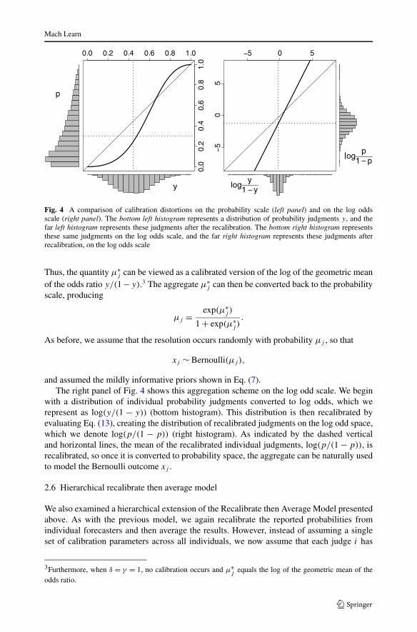
To illustrate the problem, the left panel of Fig. 4 shows a distribution of individual prob-ability judgments, represented as y (bottom histogram). After recalibrating these judgmentsvia a LLO recalibration curve with γ = 2 and δ = 0.5, the resulting distribution is repre-sented as p (the far left histogram).
The means of the uncalibrated judgments is represented as the vertical dashed line andthe mean of the recalibrated judgments is represented as the horizontal dashed line. If theaverage of p was a fully recalibrated (i.e., with respect to the event outcome) version of y,the horizontal line would intersect with the vertical line at a point directly on the recalibra-tion curve. The figure shows that although the difference is slight, the average of p is nota recalibrated version of y. Therefore, by first recalibrating individual judgments and thenaveraging the resulting recalibrated judgments, the average may not be recalibrated.2
To remedy the problem of uncalibrated aggregate predictions, we investigated a methodof aggregation on the log odds scale, where the LLO calibration function becomes linear.For a given judgment yi,j , we first recalibrate the judgment on the log odds scale, so that
pi,j = γ log
(yi,j
1 − yi,j
)+ log(δ). (13)
This transformation converts the judgments yi,j to recalibrated judgments pi,j ∈ (−∞,∞).We now have recalibrated judgments that are linear with respect to log[yi,j /(1 − yi,j )]. Wecan now aggregate these judgments in the log odds scale
μ∗j = 1
Sj
∑i∈Qj
pi,j .
1Producing an uncalibrated model prediction by aggregating calibrated forecasts is an example of Jensen’sinequality.2The judgments are always fully recalibrated in the trivial case when γ = δ = 1.
Mach Learn
Fig. 4 A comparison of calibration distortions on the probability scale (left panel) and on the log oddsscale (right panel). The bottom left histogram represents a distribution of probability judgments y, and thefar left histogram represents these judgments after the recalibration. The bottom right histogram representsthese same judgments on the log odds scale, and the far right histogram represents these judgments afterrecalibration, on the log odds scale
Thus, the quantity μ∗j can be viewed as a calibrated version of the log of the geometric mean
of the odds ratio y/(1 −y).3 The aggregate μ∗j can then be converted back to the probability
scale, producing
μj = exp(μ∗j )
1 + exp(μ∗j )
.
As before, we assume that the resolution occurs randomly with probability μj , so that
xj ∼ Bernoulli(μj ),
and assumed the mildly informative priors shown in Eq. (7).The right panel of Fig. 4 shows this aggregation scheme on the log odd scale. We begin
with a distribution of individual probability judgments converted to log odds, which werepresent as log(y/(1 − y)) (bottom histogram). This distribution is then recalibrated byevaluating Eq. (13), creating the distribution of recalibrated judgments on the log odd space,which we denote log(p/(1 − p)) (right histogram). As indicated by the dashed verticaland horizontal lines, the mean of the recalibrated individual judgments, log(p/(1 − p)), isrecalibrated, so once it is converted to probability space, the aggregate can be naturally usedto model the Bernoulli outcome xj .
2.6 Hierarchical recalibrate then average model
We also examined a hierarchical extension of the Recalibrate then Average Model presentedabove. As with the previous model, we again recalibrate the reported probabilities fromindividual forecasters and then average the results. However, instead of assuming a singleset of calibration parameters across all individuals, we now assume that each judge i has
3Furthermore, when δ = γ = 1, no calibration occurs and μ∗j
equals the log of the geometric mean of theodds ratio.
Mach Learn
a different calibration function associated with her own parameter set, thereby allowing usto capture individual differences. In the context of calibration, hierarchical models havebeen shown to drastically improve the interpretation and precision of inferential analyses inexperimental studies (e.g., Budescu and Johnson 2011; Merkle et al. 2011).
Similar to the Calibrate then Average model above, for the Hierarchical Recalibrate thenAverage model, we first recalibrate each judge’s response yi,j through the LLO function (seeEq. (2)), so that
pi,j = c(yi,j |γi, δi),
where the parameters γi and δi are the recalibration parameters for the ith judge. Notethat this is different from the Calibrate then Average model, where we assumed a singleγ and δ across all judges. As a result, we cannot simply aggregate the pi,j s and connectthe aggregate to the event resolution vector xj (see Eq. (11)) because we will be unable toestimate each individual judge’s calibration parameters. Because of the dimension mismatchbetween the matrices p and x, to connect these matrices in the model we must define anauxiliary matrix x∗ whose individual elements x∗
i,j contain the event resolution informationfor the ith judge on the j th item. Here we make a distinction between the generative processand the inferential process. By creating the auxiliary matrix x∗, the generative process wouldallow for different event resolution information for each individual judge. This feature of themodel would be useful if we were interested in examining the effects of accurate feedbackon the calibration parameters. However, in this article we assume in the inferential processthat the event resolution is the same for each individual judge such that
x∗1,j = x∗
2,j = · · · = x∗Sj ,j = xj
for all Sj judges who responded to Item j . We assume that the answer to the j th resolvedevent (for the ith judge) is a Bernoulli random variable distributed with probability equal topi,j , or
x∗i,j ∼ Bernoulli(pi,j ).
Defining the model in this way allows the calibrated judgments pi,j to vary from one judgeto another while holding the event resolutions to be the same across judges. In other words,pi,j is the model’s estimate of Judge i’s probability that Event j will occur, and therefore pi,j
models the Bernoulli process for that judge and item. We assume the calibration parametersare commonly distributed according to one hyper-distribution, so that
γi ∼ Γ (γα, γβ), and
δi ∼ Γ (δα, δβ).
After some inspection, we arrived at the following mildly informative priors for the hyper-parameters:
δα ∼ Γ (1000,1000),
γα ∼ Γ (1000,1000),
δβ ∼ Γ (1000,1000) and
γβ ∼ Γ (1000,1000).
Mach Learn
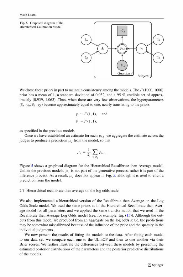
Fig. 5 Graphical diagram of theHierarchical Calibration Model
We chose these priors in part to maintain consistency among the models. The Γ (1000,1000)
prior has a mean of 1, a standard deviation of 0.032, and a 95 % credible set of approx-imately (0.939, 1.063). Thus, when there are very few observations, the hyperparameters(δα, γα, δβ, γβ ) become approximately equal to one, nearly translating to the priors
γi ∼ Γ (1,1), and
δi ∼ Γ (1,1),
as specified in the previous models.Once we have established an estimate for each pi,j , we aggregate the estimate across the
judges to produce a prediction μj from the model, so that
μj = 1
Sj
∑i∈Qj
pi,j .
Figure 5 shows a graphical diagram for the Hierarchical Recalibrate then Average model.Unlike the previous models, μj is not part of the generative process, rather it is part of theinference process. As a result, μj does not appear in Fig. 5, although it is used to elicit aprediction from the model.
2.7 Hierarchical recalibrate then average on the log odds scale
We also implemented a hierarchical version of the Recalibrate then Average on the LogOdds Scale model. We used the same priors as in the Hierarchical Recalibrate then Aver-age model for all parameters and we applied the same transformation that we used in theRecalibrate then Average Log Odds model (see, for example, Eq. (13)). Although the out-puts from this model are produced from an aggregate on the log odds scale, the predictionsmay be somewhat miscalibrated because of the influence of the prior and the sparsity in theindividual judgments.
We now present the results of fitting the models to the data. After fitting each modelto our data set, we compare each one to the ULinOP and then to one another via theirBrier scores. We further illustrate the differences between these models by presenting theestimated posterior distributions of the parameters and the posterior predictive distributionsof the models.
Mach Learn
3 The data
To test the models’ aggregation abilities, we use data collected by the Aggregative Contin-gent Estimation System (ACES), a large-scale project for collecting and combining forecastsof many widely-dispersed individuals (http://www.forecastingace.com/aces). A preliminarydescription of the data collection procedure can be found in Warnaar et al. (2012). Volunteerparticipants were asked to estimate the probability of various future events’ occurrences,such as the outcome of presidential elections in Taiwan and the potential of a downgrade ofGreek sovereign debt. Participants were free to log on to the website at their convenienceand forecast any items of interest. The forecasting problems involved events with two out-comes (event X will occur or not) as well as more than two outcomes (e.g., event A, B, orC will occur). For this paper, we focused on a subset of 176 resolved forecasting problemsthat met a number of constraints. First, they involved binary events only because we areonly considering calibration models for binary events. Second, all 176 forecasting problemsinvolved a standard way of framing the event and was presented in the form: will event Xhappen by date Y? This last constraint excluded a small number of events where the eventwas framed in terms of a deviation from status quo (e.g. will X remain true by date Y?).Finally, we only included forecasting problems where the event of interest could happen atany time before the deadline associated with the event. For example, in the event “Greecewill default on its debt in July 2011”, the target event could have occurred anytime beforethe end of July (it did not). However, items such as “The Cowboys and Aliens comic bookmovie will out-gross the Green Lantern movie on its opening weekend July 29th”, were notincluded because the event cannot happen on any other day except July 29th. These latteritems were excluded as a result of their framing because their status quo could not be altered.A total of 1401 participants contributed judgments to these forecasting problems.
3.1 Model scoring through cross-validation
We primarily evaluate models through use of the Brier score (Armstrong 2001; Brier 1950;Murphy 1973). The scoring rules that are commonly used in forecasting are often calledloss functions in the machine learning literature (e.g., Hastie et al. 2009). Popular loss func-tions for binary forecasts include squared-error loss and the (negative of the) Bernoulli log-likelihood, which forecasting researchers sometimes call the “Brier score” and “logarithmicscore,” respectively. These loss functions have the desirable property that they are “strictlyproper” (see, e.g., O’Hagan et al. 2006), meaning that the forecaster minimizes her expectedloss only by reporting her true beliefs. The expected loss cannot be reduced under alter-native strategies, such as reporting forecasts that are more extreme than one’s true beliefs.The above loss functions have also been shown to generally yield similar conclusions in aforecasting context (e.g., Staël von Holstein 1970), leading us to focus on the Brier score(squared error loss) in this paper.4
Because all events involved only two outcomes, the Brier score for the j th event can beexpressed as
Bj = (Xj − μ̂j )2,
4We also evaluated the models with both spherical and logarithmic scoring rules. However, because the resultswere invariant to these scoring rules (also see Staël von Holstein 1970), we present only the results using theBrier score.
where μ̂j is the model prediction for event j ’s occurrence and Xj is the resolution of thej th event. For example, if the j th event did occur, then Xj = 1. Thus, in this definition ofthe Brier score, the best score Bj is zero, and the worst possible score is one.
We calculate the Brier scores in a 10-fold cross-validation procedure where the parame-ters of the calibration models are estimated on a subset of 90 % of the forecasting problems.For the remaining 10 % of forecasting problems, the resolution is withheld from the model,and the calibration models are used to make the predictions μ̂j for only that subset of fore-casting problems. In the 10-fold cross-validation procedure, this process of estimation andprediction is repeated on 10 random and non-overlapping partitions of the data set to createa full set of model predictions μ̂j .
After the out-of-sample Brier scores are obtained for each event, we compute the meanpredictive error (MPE) by averaging the Brier scores across the number of events J , so
MPE = 1
J
J∑j=1
Bj .
Once the MPE scores are calculated for each model, we evaluate the percentage improve-ment over a baseline model, which in our case is the unweighted linear average (ULinOP).We calculate the percentage difference of the mean (PDM) in MPE for the ith model, de-noted MPE(i) relative to the score for the ULinOP MPE(0), by calculating
PDM = 100 × MPE(0) − MPE(i)
MPE(0). (14)
Therefore, PDM values larger than 0 indicate that the calibration model improves over theaverage prediction of the unweighted linear average (ULinOP).
In addition to the global measures of model performance given by MPE and PDM, wewill also compare models at the individual event level using a pair-wise procedure proposedby Broomell et al. (2011). In this procedure, we calculate PW(a, b), the number of eventsfor which model a has a lower Brier score than model b
PW(a, b) =J∑
j=1
1Ba,j <Bb,j(15)
where Ba,j is the Brier score for the j th event for model a, and 1x is an indicator function.This pair-wise comparison is useful because one model might have a higher MPE relative toanother model but still be the better model in the pair-wise comparison. Therefore, the MPEscore measures how well the model performs on average, whereas the PW score measuresrelative model performance on an individual event basis.
To fit all the models, we used the program JAGS (Plummer 2003) to estimate the jointposterior distribution of each set of model parameters (code for the models appears in theappendices). For each model, we obtained 1,000 samples from the joint posterior after aburn-in period of 1,000 samples, and we also collapsed across two chains. For the Recali-brate then Average and Average then Recalibrate models we initialized each of the chains bysetting γ = 0.17 and δ = 0.34. For the Hierarchical Calibration model, we initialized eachof the chains by setting γα = δα = 3 and γβ = δβ = 6.
Mach Learn
Fig. 6 Posterior predictive distributions for each of the three single-level models: Average then Recalibrate(left panel), Recalibrate then Average (middle panel), and the Recalibrate then Average Log Odds (rightpanel). The median and 95 % credible set for the posterior predictive distributions are shown as the solidblack and dashed gray lines, respectively
4 Results
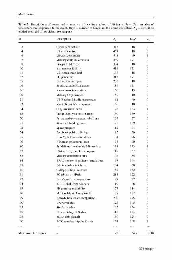
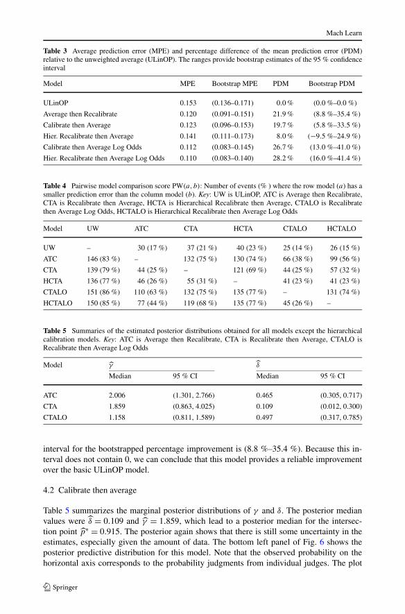
Table 2 shows a subset of 40 representative forecasting problems. For each problem, a shortdescription of the event is given, as well as the number of judges (Sj ), the number of daysthat the event was active (Days), and the resolution of the event (Xj ). Table 3 summarizesmodel performance with the average Brier score (MPE), and the percentage improvementover the baseline model (PDM). The table also shows the 95 % confidence interval forthe MPE and PDM, which we obtained by a bootstrapping procedure. The bootstrappingwas performed by repeatedly sampling forecasting problems and calculating performancestatistics on subsets of the forecasting problems in a 10-fold cross validation analysis. In thesections below, we first describe the performance of each individual model in detail and thendiscuss the pair-wise comparison scores (PW) between models (Table 4).
4.1 Average then recalibrate model
To evaluate the model, we first examined the posterior distribution of the parameters andthe posterior predictive distributions of the model. Table 5 summarizes the marginal distri-butions of γ and δ by providing the median and 95 % Bayesian credible set. The estimatesshow that there is still a good deal of uncertainty about these parameters, especially giventhe amount of data. The left panel of Fig. 6 shows the posterior predictive distribution. Toplot this distribution, we took 1,000 samples from the estimated joint posterior distributionand produced a calibration function using Eq. (2). We then plotted the median (black line)and 95 % credible set (gray lines).
Note that the model predictions of the ULinOP and the Average then Recalibrate modelare connected directly through the LLO function (see Eq. (2)). Therefore, the observed prob-ability in the left panel of Fig. 6 corresponds to the ULinOP prediction and demonstratesthat the distortion pattern for probability judgments that was found at the level of individualjudges was also found at the aggregate level (i.e., overestimation of unlikely future eventsand underestimation of likely future events). The posterior median of the intersection pointp̂∗ = 0.679 (from Eq. (3)), so that ULinOP estimates below 0.7 are mapped to smaller valuesand ULinOP estimates above 0.7 are mapped to larger values.
Table 3 shows that the MPE for the Average then Recalibrate Model is 0.12, which is21.9 % better than ULinOP. The far right column of Table 3 shows that the 95 % confidence
Mach Learn
Table 2 Descriptions of events and summary statistics for a subset of 40 items. Note: Sj = number offorecasters that responded to the event, Days = number of Days that the event was active, Xj = resolution(coded event did (1) or did not (0) happen)
Id Description Sj Days Xj
3 Greek debt default 343 18 04 US credit rating 437 18 06 Libya’s Leadership 448 49 17 Military coup in Venzuela 369 171 08 Troops to Mexico 384 18 0
Table 3 Average prediction error (MPE) and percentage difference of the mean prediction error (PDM)relative to the unweighted average (ULinOP). The ranges provide bootstrap estimates of the 95 % confidenceinterval
Model MPE Bootstrap MPE PDM Bootstrap PDM
ULinOP 0.153 (0.136–0.171) 0.0 % (0.0 %–0.0 %)
Average then Recalibrate 0.120 (0.091–0.151) 21.9 % (8.8 %–35.4 %)
Calibrate then Average 0.123 (0.096–0.153) 19.7 % (5.8 %–33.5 %)
Hier. Recalibrate then Average 0.141 (0.111–0.173) 8.0 % (−9.5 %–24.9 %)
Calibrate then Average Log Odds 0.112 (0.083–0.145) 26.7 % (13.0 %–41.0 %)
Hier. Recalibrate then Average Log Odds 0.110 (0.083–0.140) 28.2 % (16.0 %–41.4 %)
Table 4 Pairwise model comparison score PW(a, b): Number of events (% ) where the row model (a) has asmaller prediction error than the column model (b). Key: UW is ULinOP, ATC is Average then Recalibrate,CTA is Recalibrate then Average, HCTA is Hierarchical Recalibrate then Average, CTALO is Recalibratethen Average Log Odds, HCTALO is Hierarchical Recalibrate then Average Log Odds
Table 5 Summaries of the estimated posterior distributions obtained for all models except the hierarchicalcalibration models. Key: ATC is Average then Recalibrate, CTA is Recalibrate then Average, CTALO isRecalibrate then Average Log Odds
Model γ̂ δ̂
Median 95 % CI Median 95 % CI
ATC 2.006 (1.301, 2.766) 0.465 (0.305, 0.717)
CTA 1.859 (0.863, 4.025) 0.109 (0.012, 0.300)
CTALO 1.158 (0.811, 1.589) 0.497 (0.317, 0.785)
interval for the bootstrapped percentage improvement is (8.8 %–35.4 %). Because this in-terval does not contain 0, we can conclude that this model provides a reliable improvementover the basic ULinOP model.
4.2 Calibrate then average
Table 5 summarizes the marginal posterior distributions of γ and δ. The posterior medianvalues were δ̂ = 0.109 and γ̂ = 1.859, which lead to a posterior median for the intersec-tion point p̂∗ = 0.915. The posterior again shows that there is still some uncertainty in theestimates, especially given the amount of data. The bottom left panel of Fig. 6 shows theposterior predictive distribution for this model. Note that the observed probability on thehorizontal axis corresponds to the probability judgments from individual judges. The plot
Mach Learn
again shows a slowly-graded curve indicating that individual judges dramatically overesti-mated the probability of future events but showed very little underestimation.
The bottom right panel of Fig. 6 shows the posterior predictive distribution for the Re-calibrate then Average Log Odds model. It is apparent that the calibration curves for theCTA and the CTALO models are very different. For the log odds version, the median of themarginal posterior distributions (reported in Table 5) are δ̂ = 0.497 and γ̂ = 1.158, whichleads to a posterior median for the intersection point p̂∗ = 0.915. Comparing the two cal-ibration functions in the bottom panel of Fig. 6, we see that the probability scale versionapplies a stronger correction for intermediate probability judgments, pushing them down-ward toward zero.
The bottom left panel of Fig. 6 emphasizes the need to consider calibration functionsthat are not probability functions. The fits to this data clearly suggest that the judges in theexperiment are subcertain. That is, judges are overly confident in their responses relativeto observed outcome frequencies. Furthermore, judges are miscalibrated because the cred-ible intervals of the posterior predictive distributions do not capture the point (0.5,0.5).Undoubtedly, a large reason for the subcertainty is that for most resolved events, the eventdid not occur. This causes the model to favor a curve that only slowly increases c(p) as afunction of the observed probability estimates.
Table 3 shows that the Recalibrate then Average model had a MPE score of 0.123, whichis an 19.7 % improvement over the ULinOP model. The Recalibrate then Average modelwith Log Odds averaging had a MPE score of 0.112, which is an 26.7 % improvement overthe ULinOP model. Therefore, we obtain a greater improvement in model performance byusing the log odds averaging approach. For both models, the 95 % confidence interval forthe percentage improvement does not contain zero, which indicates that these models areperforming significantly better than the basic unweighted average model.
4.3 A hierarchical recalibrate then average model
To evaluate the hierarchical recalibrate then average model, we examined the posterior pre-dictive distribution and the joint posterior distribution of the parameters. Figure 7 shows theposterior predictive distribution for six judges: i = {75,139,276,1243,1393,1394}. To plotthese distribution, we took 1,000 samples from the estimated joint posterior distribution for(γi, δi), and then converted the observed yi,j s by using Eq. (2). The figure clearly showsthe individual differences between the judges. For example, Judge 1243 has a very differentcalibration function than Judges 75 and 139. Specifically, when Judge 1243 provided smallprobability forecasts (e.g., 0.1), the calibration curve pushed this probability upward andwhen he or she provided large probabilities (e.g., 0.8), the fitted calibration curve pushedthis probability downward. However, the opposite pattern occurred for Judges 75 and 139.Figure 7 also shows that some judges were well-calibrated (e.g., Judge 276). We shouldemphasize that all but one of these judges (i.e., except Judges 1243 and 276) showed clearpatterns of subcertain responding and the curves are not symmetrical.
As previously mentioned, one benefit of the hierarchical model is that it includes indi-vidual differences, allowing for much more flexible calibrations. Another substantial benefitof this model (and hierarchical Bayesian models in general) is that when there are only afew observations, the model “borrows” power from the estimates of the other judges in thesample. For example, Judges 1393 and 1394 both responded to only one item in the set. Asa consequence, the estimates of γ and δ for these judges are reflective of the prior distribu-tion for the group, which is governed by the parameters δα, γα, δβ , and γβ . Because thesehierarchical parameters are informed by all of the individual estimates for each judge in the
Mach Learn
Fig. 7 Illustrative examples for the Hierarchical Recalibrate then Average model. The median (black lines)and 95 % credible interval (gray lines) for the posterior predictive distribution for nine judges in the data set
group, when there is little information for an individual judge, the model relies more heavilyon the prior estimates for these judges.
To further illustrate the range of individual differences across judges, we compared themean of the posterior distributions for γi and δi for each judge. The top left and bottom rightpanels of Fig. 8 show the marginal distributions of γ and δ, respectively, and the top rightand bottom left panels of Fig. 8 show the joint distributions of the estimates. Judges 75, 95,139, and 1243 are shown by the filled square, circle, triangle and diamond, respectively, andJudges 1393 and 1394 are represented by the asterisk symbol. Because Judges 1393 and1394 have so few observations, their estimates are most similar to the priors, where there isa heavy concentration of estimates (see the marginal distributions of γ and δ in Fig. 8).
The Hierarchical Recalibrate then Average model without log odds averaging obtained aMPE of 0.141, which is a 8 % improvement over the ULinOP. However, the Hierarchical Re-calibrate then Average model with Log Odds averaging obtained a MPE of 0.110, which isa 28.2 % improvement over the ULinOP. The model performance of the hierarchical modelwith log odds averaging is slightly better than the non-hierarchical version. However, thisdifference is small (and the pair-wise comparisons shown later will not show an advantagefor the hierarchical model). Therefore, this suggests that although the modeling of individualdifferences does not provide a substantial improvement in prediction performance.
4.4 Model comparison at the individual event level
Overall, based on the average prediction error (MPE), it appears that the Hierarchical Re-calibrate then Average Log Odds model is the best performing model among all the models
Mach Learn
Fig. 8 The marginal (top leftand bottom right panels) andjoint (top right and bottom leftpanels) distributions of the meanestimates for the 1401 judges inthe experiment for theHierarchical Recalibrate thenAverage model. Judges 75, 95,139, and 1243 are shown by thefilled square, circle, triangle anddiamond, respectively, andJudges 1393 and 1394 arerepresented by the asterisksymbol
that we examined. However, this global measure of model prediction error ignores some im-portant patterns at the individual event level (Broomell et al. 2011). For example, one modelcan achieve a low MPE relative to another model by having substantially better Brier scoreson a few forecasting problems, while still doing more poorly on a majority of the problems.The pair-wise model comparison score discussed above emphasizes the latter form of modelimprovement because it measures the number of forecasting problems on which one modelis better than another, regardless of the magnitude of the improvement.
Table 4 shows the pair-wise model comparison scores between six models of interestin the cross validation procedure. Each element in the table shows the number of timesthe model corresponding to the row fit the data better than the model corresponding to thecolumn, and the percentages are shown in the parentheses. Because the CTALO (Recalibratethen Average Log Odds) model is the only model whose rows contains percentages that areall above 50 %, it is the best performing model in this pair-wise comparison. Importantly,the CTALO model outperforms the hierarchical extension of this model (HCTALO) in 131out of 176 forecasting problems (74 %).
5 General discussion
In this article, we have examined several models that use the “linear in log odds” function(see Eq. (2)) to recalibrate individual or average judgments and improve the prediction offuture events. We found that the order and type of calibration and aggregation had a largeimpact on the model performance. Overall, in the pair-wise model comparison we found thatthe Recalibrate then Average Log Odds model has a lower prediction error than any othermodel on the majority of events. It also performs only slightly worse than the HierarchicalRecalibrate then Average Log Odds model on the average prediction error. Therefore, weconclude that Recalibrate then Average Log Odds model is the simplest and best approachto aggregate forecasting judgments in the presence of systematic biases.
Mach Learn
As mentioned in the introduction, in comparing the models we contrasted the conse-quences of a number of modeling assumptions, including (1) the point at which recalibrationoccurs (before or after aggregation), (2) the space in which the recalibration and aggregationshould take place, (3) the extent to which individual differences are taken into account. Ourmain goal was to assess how these different assumptions affected the model performance.We now discuss each of these topics in turn and also discuss the influence of the codingscheme for events.
5.1 The order of aggregation and calibration
Our first research question was whether it is better to first aggregate and then recalibrateor recalibrate then average. The answer is that it depends on whether it is probabilities orlog-odds that are being averaged. Working solely in the probability scale, we obtained betterresults in comparisons against the ULinOP when averaging first than when calibrating first(compare rows 2 and 4 in Table 3 and the first two cells under UW in Table 4). However,when averaging log-odds, it is better to calibrate first (row 6 in Table 3 and cell 5 under UWin Table 4).
5.2 The aggregation space
We then compared working with probability and log-odds scales and found that aggregatingon the log odds instead of the probability scale led to a reversal in the order of the aggre-gation and calibration methods to achieve the best results. Specifically, the Recalibrate thenAverage Log Odds model outperformed the ULinOP by 26.7 %, and achieved the secondbest MPE score at 0.112. Taking these new results into account, our conclusion above wasreversed: it is better to first recalibrate the individual judgments and then aggregate theserecalibrated values on the log odds scale.
5.3 The inclusion of individual differences
We examined the benefits of including individual differences in the models. Both of our hier-archical models assigned separate calibration parameters for each individual and estimatedthe individual parameters in a hierarchical Bayesian approach. This allowed for the estima-tion of these parameters even for individuals who contributed only a few judgments. Forthe Hierarchical Recalibrate then Average Log Odds model, we found that taking individualdifferences into account when aggregating probability judgments led to a 1.5 % improve-ment in the PDM. However, in the pair-wise comparisons, the hierarchical model performedsystematically worse than the non-hierarchical model equivalent (the Recalibrate then Aver-age Log Odds Models). This shows that the any modeling advantage from the hierarchicalmodel comes from improved performance on a small number of forecasting problems andnot a systematic improvement across the majority of forecasting problems.
5.4 The role of coding
Finally, we discuss the role of coding. Although the LLO function is not a probability func-tion, we still will work with probabilities in binary forecasts. For example, suppose p is theelicited (and possibly aggregated) probability for the occurrence of some event of interest,we can use c(p) for the transformed probability of an event happening and 1 − c(p) for theprobability that an event will not happen. Alternatively, we can use a reverse coding scheme
Mach Learn
where p is the probability for the occurrence of some event, 1 − p is the judgment elicited,1 − c(1 − p) for the transformed probability of an event happening, and c(1 − p) for thetransformed probability that an event will not happen. The reverse coding scheme will notaffect the performance of the models because the transformation still maps to a particularcalibration function, specifically
1 − c(1 − p|γ, δ) = pγ
δ(1 − p)γ + pγ
= c(p|γ,1/δ).
In the Bayesian framework, for the performance results to be exact, the contribution ofthe prior for the regular coding scheme must be equivalent to contribution of the prior forthe reverse coding scheme for the parameter δ (i.e., the prior for γ can remain the same).For example, for the Average then Calibrate Model we specified that δ ∼ Γ (α,β), whereα = β = 1. In the reverse coding scheme, an equivalent prior for 1/δ is the inverse gammadistribution, such that 1/δ ∼ Γ −1(α,1/β). Thus, with the appropriate selection of the priordistribution, the particular coding of the responses and event resolutions has no effect onmodel performance when using the LLO function.
5.5 Alternatives
There are several other model-based approaches that should be examined and consideredin future work. They are important because they provide a model for the internal repre-sentation of the judge, which recalibration functions neglect. For example, the DecisionVariable Partition model (Ferrell and McGoey 1980) uses signal detection theory as a baserepresentation of the underlying distributions for the alternatives. While this model pro-vides a generally adequate fit to the data (e.g., Suantak et al. 1996), it has been criti-cized by Keren (1991) for not providing a description of the cognitive processes under-lying confidence. However, more recent models have taken this general approach but pro-vide possible explanations of the underlying cognitive processes (e.g., Jang et al. 2012;Wallsten and González-Vallejo 1994).
Other models assume that the judge has a perfectly accurate representation of the ob-served relative frequency, but due to random error, the probability elicited by the judge isa distorted and usually inaccurate version of the observed relative frequency. Erev et al.(1994) demonstrated through simulation that models of this type can produce typical over-confidence patterns in the data. Other models in this general framework assume the error isattributable to the judgment (the stochastic judgment model; Wallsten and González-Vallejo1994), aspects of the environment (the ecological error model; Soll 1996) or both (e.g.,Juslin and Olsson 1997).
Finally, there exist a variety of mathematical models that explicitly describe psychologi-cal processes underlying confidence and/or subjective probability. These include the Poissonrace model (Merkle and Van Zandt 2006; Van Zandt 2000), HyGene (Thomas et al. 2008),and the two-stage dynamic signal detection model (Pleskac and Busemeyer 2010).
Although these model-based approaches are important because they offer informationabout the underlying processes driving the decision, for the sake of simplicity we did not in-clude them in this comparison that focuses primarily on maximizing the predictive accuracyof group forecasts.
Mach Learn
6 Conclusions
We have demonstrated that several aggregation methods surpass the predictive accuracy ofthe ULinOP, at least in the limited situation of forecasting whether or not the status quo willchange within a specified time frame. Our best performing model first corrected for sys-tematic distortions and then aggregated the calibrated judgments on the log odds scale. Thehierarchical version of the calibration model, which allowed for individual differences in thenature of the systematic distortion, outperformed its single-level counterpart, but this differ-ence was small; and we concluded for this study does not merit the additional complexityinvolved.
The present work builds on a growing body of literature evaluating various calibrationand aggregation methods. Aggregating multiple subjective probability estimates to improvethe performance of the estimate ties into the concept of the “wisdom of the crowd” effect(Surowiecki 2004), which has usually been studied in the context of a single magnitude esti-mate. For example, Galton (1907) found that when people were asked to estimate the weightof a butchered ox, the average of these estimates was almost exactly correct, despite widevariability in the estimates. More recent studies have demonstrated this effect in more com-plicated situations such as optimizing solutions in combinatorial problems (Yi et al. 2010;Yi et al. 2011), inferring expertise (Lee et al. 2011), maximizing event recall accuracy (Hem-mer et al. 2011) and solving ordering problems (Miller et al. 2009; Steyvers et al. 2009). Thepresent work suggests substantially greater improvement can be attained by taking system-atic distortions in the individual judgments into account. The best aggregation performancemight be obtained with models that first recalibrate individual estimates and then combinethese recalibrated judgments on an appropriate scale.
Acknowledgements Supported by the Intelligence Advanced Research Projects Activity (IARPA) via De-partment of Interior National Business Center (DoI/NBC) contract number D11PC20059. The US Govern-ment is authorized to reproduce and distribute reprints for Governmental purposes notwithstanding any copy-right annotation thereon. Disclaimer: The views and conclusions contained herein are those of the authors andshould not be interpreted as necessarily representing the official policies or endorsements, either expressed orimplied, of IARPA, DoI/NBC, or the US Government.
Appendix
In each of the JAGS codes below, we pass the program a series of data structures to facilitatethe estimations. For all of the single-level models, we let y contain all probability judgments,so it is a vector containing all of the judgments for the first item, followed by the seconditem, and so on. To tell the program when the responses change from one item to the next,we pass it a vector containing these indexes, called nresps. For example, nresps[1] mightequal 740, which indicates that all of the responses from y[1] to y[740] are for the firstitem. For the Average then Recalibrate model, y contains only the averages of all judgmentsfor each item, so nresps is not needed. For the hierarchical models, y is a matrix wherethe rows correspond to the observation, the first column contains the subject index elicitingthe judgment, and the second column contains the judgment. In addition, we pass JAGSa new variable xstar, which contains the event resolution information for each individualseparately (see text above).
Finally, we pass the program the upper indexes for each loop. We let nd be the totalnumber of probability judgments, nq be the number of items in the set, nk is the number ofitems with known outcomes, and ns is the number of subjects (only used for the hierarchicalmodels). For the hierarchical models, nk is the number of responses to items having knownoutcomes (i.e., nk is the length of the vector xstar).
Mach Learn
A.1 Calibrate then average
##### Recalibrate Then Averagemodel{# Specify the recalibration functionfor(k in 1:nd){p[k] <-delta*(y[k])^gamma/(delta*(y[k])^gamma+(1-y[k])^gamma)}# Collapse the information in the p matrix through aggregationmu[1] <- mean(p[1:nresps[1]])for(j in 2:nq){mu[j] <- mean(p[(1+nresps[j-1]):nresps[j]])}# The resolution is a result of the latent mean parametersfor(j in 1:nk){x[j] ~ dbern(mu[j])}# Priors on model parametersdelta ~ dgamma(1,1)gamma ~ dgamma(1,1)}
A.2 Calibrate then average log odds scale
##### Recalibrate Then Average Log Odds Scalemodel{# Specify the recalibration functionfor(k in 1:nd){p[k] <- gamma*log(y[k]/(1-y[k])) + log(delta)}# Collapse the information in the p matrix through aggregationmu_star[1] <- mean(p[1:nresps[1]])mu[1] <- exp(mu_star[1])/(1+exp(mu_star[1]))for(j in 2:nq){mu_star[j] <- mean(p[(1+nresps[j-1]):nresps[j]])mu[j] <- exp(mu_star[j])/(1+exp(mu_star[j]))}# The resolution is a result of the latent mean parametersfor(j in 1:nk){x[j] ~ dbern(mu[j])}# Priors on model parametersdelta ~ dgamma(1,1)gamma ~ dgamma(1,1)}
A.3 Average then recalibrate
##### Average then Recalibratemodel{# Specify recalibration function
Mach Learn
for(k in 1:nq){p[k] <- delta*(y[k])^gamma/(delta*((y[k])^gamma)+(1-y[k])^gamma)}# The resolution is a result of the latent mean parametersfor(j in 1:nk){x[j] ~ dbern(p[j])}# Priors on model parametersdelta ~ dgamma(1,1)gamma ~ dgamma(1,1)}
A.4 Hierarchical recalibrate then average
##### Hierarchical Recalibrate then Averagemodel{# Specify recalibration functionfor(k in 1:nd){p[k] <- delta[y[k,1]]*(y[k,2])^gamma[y[k,1]]/(delta[y[k,1]]*(y[k,2])^gamma[y[k,1]]+(1-y[k,2])^gamma[y[k,1]])}# The resolution is a result of the latent mean parametersfor(j in 1:nk){xstar[j] ~ dbern(p[j])}# Priors on individual-level model parametersfor(i in 1:ns){delta[i] ~ dgamma(delta_mu,delta_sigma)gamma[i] ~ dgamma(gamma_mu,gamma_sigma)}# Priors on hyperparametersdelta_mu ~ dgamma(1000,1000)gamma_mu ~ dgamma(1000,1000)delta_sigma ~ dgamma(1000,1000)gamma_sigma ~ dgamma(1000,1000)}
A.5 Hierarchical recalibrate then average log odds
##### Hierarchical Recalibrate then Average Log Oddsmodel{# Specify recalibration functionfor(k in 1:nd){p[k] <- gamma[y[k,1]]*log(y[k,2]/(1-y[k,2])) + log(delta[y[k,1]])}# Aggregate the p vectormu_star[1] <- mean(p[1:nresps[1]])mu[1] <- exp(mu_star[1])/(1+exp(mu_star[1]))for(j in 2:nq){mu_star[j] <- mean(p[(1+nresps[j-1]):nresps[j]])mu[j] <- exp(mu_star[j])/(1+exp(mu_star[j]))
Mach Learn
}# The resolution is a result of the latent mean parametersfor(j in 1:nk){xstar[j] ~ dbern(mu[j])}# Priors on individual-level model parametersfor(i in 1:ns){delta[i] ~ dgamma(delta_mu,delta_sigma)gamma[i] ~ dgamma(gamma_mu,gamma_sigma)}# Priors on hyperparametersdelta_mu ~ dgamma(1000,1000)gamma_mu ~ dgamma(1000,1000)delta_sigma ~ dgamma(1000,1000)gamma_sigma ~ dgamma(1000,1000)}
References
Ariely, D., Au, W. T., Bender, R. H., Budescu, D. V., Dietz, C. B., Gu, H., Wallsten, T. S., & Zauberman, G.(2000). The effects of averaging subjective probability estimates between and within judges. Journal ofExperimental Psychology. Applied, 6, 130–147.
Arkes, H. R., Dawson, N. V., Speroff, T., Harrell, F. E. Jr., Alzola, C., Phillips, R., Desbiens, N., Oye, R. K.,Knaus, W., & Connors, A. F. Jr. (1995). The covariance decomposition of the probability score and itsuse in evaluating prognostic estimates. Medical Decision Making, 15, 120–131.
Armstrong, J. S. (2001). Principles of forecasting. Norwell: Kluwer Academic.Birnbaum, M. H., & McIntosh, W. R. (1996). Violations of branch independence in choices between gambles.
Organizational Behavior and Human Decision Processes, 67, 91–110.Breiman, L. (1996). Bagging predictors. Machine Learning, 24, 123–140.Brenner, L. A., Koehler, D. J., Liberman, V., & Tversky, A. (1996). Overconfidence in probability and fre-
quency judgments: a critical examination. Organizational Behavioral and Human Decision Processes,65, 212–219.
Brier, G. W. (1950). Verification of forecasts expressed in terms of probability. Monthly Weather Review, 78,1–3.
Broomell, S. B., Budescu, D. V., & Por, H. H. (2011). Pair-wise comparison of multiple models. Judgementand Decision Making, 6, 821–831.
Brown, S., & Steyvers, M. (2009). Detecting and predicting changes. Cognitive Psychology, 58, 49–67.Budescu, D. V., & Johnson, T. R. (2011). A model-based approach for the analysis of the calibration of
probability judgments. Judgment and Decision Making, 6, 857–869.Buntine, W. L. (1994). Operations for learning with graphical models. Journal of Artificial Intelligence Re-
search, 2, 159–225.Camerer, C. F., & Ho, T. H. (1994). Violations of the betweenness axiom and nonlinearity in probability.
Journal of Risk and Uncertainty, 8, 167–196.Christensen, R., Johnson, W., Branscum, A., & Hanson, T. E. (2011). Bayesian ideas and data analysis: an
introduction for scientists and statisticians. Boca Raton: CRC Press.Christensen-Szalanski, J. J. J., & Bushyhead, J. B. (1981). Physicians’ use of probabilistic information in
a real clinical setting. Journal of Experimental Psychology. Human Perception and Performance, 7,928–935.
Clemen, R. T. (1986). Calibration and the aggregation of probabilities. Management Science, 32, 312–314.Clemen, R. T. (1989). Combining forecasts: a review and annotated bibliography (with discussion). Interna-
tional Journal of Forecasting, 5, 559–583.Clemen, R. T., & Winkler, R. L. (1986). Combining economic forecasts. Journal of Business & Economic
Statistics, 4, 39–46.Cooke, R. M. (1991). Experts in uncertainty: opinion and subjective probability in science. New York: Oxford
University Press.
Mach Learn
Erev, I., Wallsten, T. S., & Budescu, D. V. (1994). Simultaneous over- and underconfidence: The role of errorin judgment processes. Psychological Review, 101, 519–527.
Ferrell, W. R., & McGoey, P. J. (1980). A model of calibration for subjective probabilities. OrganizationalBehavior and Human Decision Processes, 26, 32–53.
Freund, Y., & Schapire, R. E. (1996). Experiments with a new boosting algorithm. In Machine learning: Pro-ceedings of the thirteenth international conference (pp. 325–332). San Francisco: Morgan Kauffman.
Fryback, D. G., & Erdman, H. (1979). Prospects for calibrating physicians’ probabilistic judgments: designof a feedback system. In Proceedings of the IEEE international conference on cybernetics and society.
Galton, F. (1907). Vox populi. Nature, 75, 450–451.Gelman, A., Carlin, J. B., Stern, H. S., & Rubin, D. B. (2004). Bayesian data analysis. New York: Chapman
and Hall.Gonzalez, R., & Wu, G. (1999). On the shape of the probability weighting function. Cognitive Psychology,
38, 129–166.Griffin, D., & Tversky, A. (1992). The weighing of evidence and the determinants of confidence. Cognitive
Psychology, 24, 411–435.Härdle, W. (1992). Applied nonparametric regression. Cambridge: Cambridge University Press.Hastie, T., Tibshirani, R., & Friedman, J. (2009). The elements of statistical learning (2nd ed.). New York:
Springer.Hemmer, P., Steyvers, M., & Miller, B. J. (2011). The wisdom of crowds with informative priors. In Proceed-
ings of the 32rd annual conference of the cognitive science society. Lawrence Erlbaum.Hora, S. C. (2004). Probability judgments for continuous quantities: Linear combinations and calibration.
Management Science, 50, 597–604.Jang, Y., Wallsten, T. S., & Huber, D. E. (2012). A stochastic detection and retrieval model for the study of
metacognition. Psychological Review, 119, 186–200.Juslin, P., & Olsson, H. (1997). Thurstonian and Brunswikian origins of uncertainty in judgment: a sampling
model of confidence in sensory discrimination. Psychological Review, 104, 344–366.Kahneman, D., & Tversky, A. (1979). Prospect theory: An analysis of decision under risk. Econometrica, 47,
263–291.Karmarker, U. S. (1978). Subjectively weighted utility: a descriptive extension of the expected utility model.
Organizational Behavior and Human Performance, 21, 61–72.Keren, G. (1991). Calibration and Probability Judgments: Conceptual and Methodological Issues. Acta Psy-
chologica.Lee, M. D. (2008). Three case studies in the Bayesian analysis of cognitive models. Psychonomic Bulletin &
Review, 15, 1–15.Lee, M. D., Steyvers, M., de Young, M., & Miller, B. J. (2011). A model-based approach to measuring
expertise in ranking tasks. In Proceedings of the 33rd annual conference of the cognitive science society.Cognitive Science Society.
Lee, M. D., & Wagenmakers, E.-J. (2012). A course in Bayesian graphical modeling for cognitive sci-ence. Available from http://www.ejwagenmakers.com/BayesCourse/BayesBookWeb.pdf; last down-loaded January 1, 2012.
Lichtenstein, S., Fischoff, B., & Phillips, L. D. (1982). Calibration of probabilities: the state of the art to 1980.In D. Kahneman, P. Slovic, & A. Tversky (Eds.), Judgment under uncertainty: heuristics and biases (pp.306–334). Cambridge: Cambridge University Press.
Merkle, E. C. (2010). Calibrating subjective probabilities using hierarchical Bayesian models. In S.-K. Chai,J. J. Salerno, & P. L. Mabry (Eds.), Lecture notes in computer science: Vol. 6007. Social computing,behavioral modeling, and prediction (SBP) 2010 (pp. 13–22).
Merkle, E. C., Smithson, M., & Verkuilen, J. (2011). Hierarchical models of simple mechanisms underlyingconfidence in decision making. Journal of Mathematical Psychology, 55, 57–67.
Merkle, E. C., & Van Zandt, T. (2006). An application of the Poisson race model to confidence calibration.Journal of Experimental Psychology. General, 135, 391–408.
Miller, B. J., Hemmer, P., Steyvers, M., & Lee, M. D. (2009). The wisdom of crowds in ordering problems.In Proceedings of the ninth international conference on cognitive modeling, Manchester, UK.
Murphy, A. H. (1973). A new vector partition of the probability score. Journal of Applied Meteorology, 12,595–600.
Murphy, A. H., & Winkler, R. L. (1974). Credible interval temperature forecasting: some experimental re-sults. Monthly Weather Review, 102, 784–794.
Murphy, A. H., & Winkler, R. L. (1984). Probability forecasting in meteorology. Journal of the AmericanStatistical Association, 79, 489–500.
O’Hagan, A., Buck, C. E., Daneshkhah, A., Eiser, J. R., Garthwaite, P. H., Jenkinson, D. J., Oakley, J. E., &Rakow, T. (2006). Uncertain judgements: eliciting experts’ probabilities. Hoboken: Wiley.
Page, L., & Clemen, R. T. (2012). Do prediction markets produce well calibrated probability forecasts?Manuscript in preparation.
Pleskac, T. J., & Busemeyer, J. R. (2010). Two-stage dynamic signal detection theory: a theory of choice,decision time, and confidence. Psychological Review, 117, 864–901.
Plummer, M. (2003). JAGS: a program for analysis of Bayesian graphical models using Gibbs sampling. InProceedings of the 3rd international workshop on distributed statistical computing.
Shiffrin, R. M., Lee, M. D., Kim, W., & Wagenmakers, E.-J. (2008). A survey of model evaluation approacheswith a tutorial on hierarchical Bayesian methods. Cognitive Science, 32, 1248–1284.
Shlomi, Y., & Wallsten, T. S. (2010). Subjective recalibration of advisors’ probability estimates. PsychonomicBulletin & Review, 17, 492–498.
Silverman, B. W. (1986). Density estimation for statistics and data analysis. London: Chapman & Hall.Soll, J. B. (1996). Determinants of overconfidence and miscalibration: the roles of random error and ecolog-
ical structure. Organizational Behavior and Human Decision Processes, 65, 117–137.Staël von Holstein, C. A. S. (1970). Measurement of subjective probability. Acta Psychologica, 34, 146–159.Steyvers, M., Lee, M. D., & Miller, B. J. (2009). Wisdom of crowds in the recollection of order information.
In Y. Bengio, D. Schuurmans, J. Lafferty, C. K. I. Williams, & A. Culotta (Eds.), Advances in neuralinformation processing systems. (Vol. 22, pp. 1785–1793). New York: MIT Press.
Suantak, L., Bolger, F., & Ferrell, W. R. (1996). The hard-easy effect in subjective probability calibration.Organizational Behavior and Human Decision Processes, 67, 201–221.
Surowiecki, J. (2004). The wisdom of crowds. New York: Random House.Thomas, R. P., Dougherty, M. R., Sprenger, A. M., & Harbison, J. I. (2008). Diagnostic hypothesis generation
and human judgment. Psychological Review, 115, 155–185.Tversky, A., & Fox, C. R. (1995). Weighing risk and uncertainty. Psychological Review, 102, 269–283.Tversky, A., & Kahneman, D. (1992). Advances in prospect theory: cumulative representations of uncertainty.
Journal of Risk and Uncertainty, 5, 297–323.Van Zandt, T. (2000). ROC curves and confidence judgments in recognition memory. Journal of Experimental
Psychology. Learning, Memory, and Cognition, 26, 582–600.Wallsten, T. S., & Budescu, D. V. (1983). Encoding subjective probabilities: a psychological and psychomet-
ric review. Management Science, 29, 151–173.Wallsten, T. S., Budescu, D. V., & Erev, I. (1997). Evaluating and combining subjective probability estimates.
Journal of Behavioral Decision Making, 10, 243–268.Wallsten, T. S., & González-Vallejo, C. (1994). Statement verification: a stochastic model of judgment and
response. Psychological Review, 101, 490–504.Warnaar, D., Merkle, E., Steyvers, S., Wallsten, T., Stone, E., Budescu, D., Yates, J., Sieck, W., Arkes, H.,
Argenta, C., Shin, Y., & Carter, J. (2012). The aggregative contingent estimation system: selecting, re-warding, and training experts in a wisdom of crowds approach to forecasting. In 2012 AAAI symposium.on Wisdom of the Crowd.
Wright, G. (1982). Changes in the realism and distribution of probability assessments as a function of questiontype. Acta Psychologica, 52, 165–174.
Wright, G., & Wisudha, A. (1982). Distribution of probability assessments for almanac and future eventquestions. Scandinavian Journal of Psychology, 23, 219–224.
Wu, G., & Gonzalez, R. (1996). Curvature of the probability weight function. Management Science, 42,1676–1690.
Yates, J. F. (1982). External correspondence: decompositions of the mean probability score. OrganizationalBehavior and Human Performance, 30, 132–156.
Yates, J. F. (1990). Judgment and decision making. Englewood Cliffs: Prentice Hall.Yi, S. K. M., Steyvers, M., & Lee, M. D. (2011). The wisdom of crowds in combinatorial problems. Cognitive
Science.Yi, S. K. M., Steyvers, M., Lee, M. D., & Dry, M. (2010). Wisdom of crowds in minimum spanning tree
problems. In Proceedings of the 32nd annual conference of the cognitive science society. LawrenceErlbaum.
Zhang, H., & Maloney, L. T. (2011). Ubiquitous log odds: a common representation of probability and fre-quency distortion in perception, action, and cognition. Frontiers in Neuroscience, 6, 1–14.