28
Forecasting
| Date post: | 23-Dec-2015 |
| Category: |
Documents |
| Upload: | sakshigupta |
| View: | 8 times |
| Download: | 0 times |

Forecasting

• Forecasting product demand is crucial to any supplier, manufacturer, or retailer.
• Forecasts of future demand will determine the quantities that should be purchased, produced, and shipped.
• Most firms cannot simply wait for demand to emerge and then react to it. Instead, they must anticipate and plan for future demand so that they can react immediately to customer orders as they occur.
• In other words, most manufacturers "make to stock" rather than "make to order" – they plan ahead and then deploy inventories of finished goods into field locations. Thus, once a customer order materializes, it can be fulfilled immediately – since most customers are not willing to wait the time it would take to actually process their order throughout the supply chain and make the product based on their order. An order cycle could take weeks or months to go back through part suppliers and sub-assemblers, through manufacture of the product, and through to the eventual shipment of the order to the customer.

• In general practice, accurate demand forecasts lead to efficient operations and high levels of customer service, while inaccurate forecasts will inevitably lead to inefficient, high cost operations and/or poor levels of customer service.
• In many supply chains, the most important action we can take to improve the efficiency and effectiveness of the logistics process is to improve the quality of the demand forecasts.

Forecasting as a planning tool
• Managerial decision making is often complicated due to an element of uncertainty in the variables affecting the decision making process.
• For example, when the decision to build a new production facility is made, the demand for its products is not known with certainty.
• Similarly, when a hospital chooses to add one more specialty healthcare wing, it needs to make some assumptions about the demand for the facility.
• Since these decisions often involve considerable cash flow and time in creating new facilities, accurate estimates of the future events for which the decisions have been made are crucial.
• Forecasts are estimates of the timings and magnitude of the occurrence of future events.
• Forecasting involves 2 important aspects-the magnitude (how much demand) and the timing of occurrence of events.

• Consider a fast food joint that operates close to a commercial centre. As large number of visitors visits commercial centre, one could expect a good demand for food and beverages. Let us suppose that the owner of the fast food joint estimates the daily demand for beverages to be 3000 cups. But this information is not sufficient. The timing of the demand is very crucial. For example if 40% of the estimated demand happens in just 2 blocks of two hours each in the morning and the evening, then the nature of planning and even operational practices during these peak hours could be very different.
• Manufacturing and service systems experience peak demand certain times and average or even low demand during other times. Hence estimation of timing is important.
• The timing is important for long term planning as well. Example if a company wants to add one more product line –microwave ovens to its product portfolio. The decision to add microwave ovens to the product line requires a good understanding of the nature of demand for the range of microwave ovens proposed to be manufactured. Depending on both the timing and the magnitude of demand, the manufacturer will schedule the building of new plants, planning of the product launch, and the creation of the necessary infrastructure for the marketing and distribution of microwave ovens.

• Even government needs forecast of population growth over the next 10-20 years in order to make long term plans for creating infrastructure for transportation and the development of cities and towns.
• Forecasting is the process of projecting the values of one or more variables into the future.
• Poor forecasting can result in poor inventory and staffing decisions, resulting in part shortages, inadequate customer service and many customer complaints.
• Accurate forecasts are needed throughout the value chain, and are used by all functional areas of the organization, including accounting, finance, marketing, operations and distribution.
• The planning horizon is the length of time on which a forecast is based. This spans from short range forecasts with a planning horizon of under 3 months to long range forecasts of 1 to 10 years.

Why do we Forecast?
• Dynamic and complex environments: Forecasting is not required if an organization has complete control over market forces and knows exactly what the sale of its products is going to be in the future. But such conditions does not exist.
• Short term fluctuations in production: A good forecasting system will be able to predict the occurrence of short term fluctuations in demand.
• Better materials management: Since the impending events in an organization are predicted through a forecasting system, organizations can benefit from better materials management and ensure better resources availability. Example- from the above example of fast food joint, if the owner could predict the occurrence of peak hours in his joint, he would have planned and ensured better material and greater availability of resources.

• Rationalized manpower decisions: A forecasting system provides useful information on the nature of the resources required and their timing and magnitude. Therefore, organizations can minimize hiring and lay-off decisions through forecasting. Moreover, better planning of overtime and idle time can also be done based on this information.
• Basis for planning and scheduling: The uses of forecasting clearly point to the fact that the planning and scheduling of activities can be done on a rational basis.
• Strategic decisions: Earlier example of microwave oven suggests that forecasting plays an important role in long term strategic decision making. This includes planning for product line decisions, new products, augmenting capacity, building new factories, and expanding the current level of activities.

Forecasting Time Horizon
Three categories are short-term, medium-term and long term horizons.
Short term Forecasting
Forecasting acts as an input for the tactical decisions that an organization makes. For example, based on the sales in the last quarter, an organization could develop better estimates of the demand in the next quarter and use that information for adjusting various quarterly plans.
Medium- term Forecasting
An organization uses forecasting as a starting point to the annual business planning exercise.This constitutes the medium term forecasting.Planning horizon is usually 12-18 months.Since the forecasting is done for a slightly longer time, cyclical and seasonal patterns will make a significant impact and need to be incorporated in the analysis.The decisions taken using the forecasting information vary from purely tactical decisions such as annual production planning to somewhat strategic ones such as augmentation of capacity in specific areas of business.
Long term Forecasting
Long term forecasts involve purely strategic decisions for a time period of about 5-10 years, so the forecasting processes need to cater to these requirements.

Models for ForecastingThe various models for forecasting can be
classified into 3 categories:-1) Extrapolative methods2) Causal methods3) Subjective judgments using qualitative data
1) Extrapolative methods
Make use of past data and prepare future estimates by some methodof extrapolating the past data.
For example, the demand for soft drinks in a city or a locality could be estimated as 110 per cent of the average sales during the last three months.
Similarly the sales of new garments during the festive season could be estimated to be a percentage of the festive season sales during the previous year.
In both the above examples we are using the past data and extrapolating it into the future on some basis.
2) Causal models
Analyse data from the viewpoint of a cause effect relationship.For example, in the process of estimating the demand for new
houses, the model will identify the factors that could influence the demand for new houses and establish the relationship between these factors and the demand.
For example, the factors may include real estate prices, housing finance options, disposable income of families, the cost of construction and benefits derived from the tax laws.
Once the relationship between these variables and the demand is established, it is possible to use it for estimating the demand for new houses.

• Subjective judgments using qualitative data An organization such as the Indian Space Research Organization
(ISRO) would use this method to forecast the technology trends in space launch vehicles and the expertise that needs to be developed in the organization over the next 10 years.
Type Characteristics Strengths WeaknessesExecutive opinion
A group of managers meet & come up with a forecast
Good for strategic or new-product forecasting
One person's opinion can dominate the forecast
Market research
Uses surveys & interviews to identify customer preferences
Good determinant of customer preferences
It can be difficult to develop a good questionnaire
Delphi method
Seeks to develop a consensus among a group of experts
Excellent for forecasting long-term product demand, technological changes, and
Time consuming to develop

A) Extrapolative Methods using Time SeriesA time series is simply a collection of data at fixed time intervals over
several years.Since extrapolative methods are estimates of future requirement on the
basis of past data, the most important requirement for extrapolative methods is the existence of past data.
Hence, this method is unsuitable for brand new products and new markets.
For example, if Tata Motors wants to estimate the demand for the Nano for the next two quarters, it is not possible to use this method.
Established product lines will have several data points of the past that could be put to use.
They are useful for short term forecasts in an organization.This includes predicting weekly/monthly demand for several fast moving
items and forecast of capacity requirements in manufacturing and service organizations.
Extrapolative models with some level of sophistication will also be useful for medium term forecasts.

i) Moving AveragesThe simplest model for extrapolative forecasting
is the method of simple moving averages.The model has a single parameter, that is, the
number of periods to be considered for computing the moving average.
For example, an organization may use a three period moving average to estimate the demand of one of its fast moving products.

3-Period and 6-Period Moving Average
(1300+1356+1442)/3 (1300+1356+1442+1576+1716+1832)/6
Week Demand3-week
MA Forecast1 13002 13563 1442 13664 1576 1458 13665 1716 1578 14586 1832 1708 15787 1996 1848 17088 2028 1952 18489 2048 2024 195210 2200 2092 202411 2214 2154 209212 2420 2278 2154
Week Demand6-week
MA Forecast1 13002 13563 14424 15765 17166 1832 15377 1996 1653 15378 2028 1765 16539 2048 1866 176510 2200 1970 186611 2214 2053 197012 2420 2151 2053

Weighted Moving AveragesWhen there is a detectable trend or pattern, weights can be used to place
more emphasis on recent values. This makes the techniques more responsive to changes since more recent periods may be more heavily weighted. Deciding which weights to use requires some experience and a bit of luck. Choice of weights is somewhat arbitrary since there is not set formula to determine them.
Advantage of moving average: Easy to use and to compute.Disadvantage: values in the average are weighted equally. For example, in a
ten- period moving averageeach the same weight of 1/10., the oldest has an equal value to the most
recent.Mathematically, Weighted Moving average = ∑ (weight for period n) x (Demand in period n) /
∑weights

Time in the past Weightage
4 years ago 0.05
3 years ago 0.25
2 years ago 0.3
Last year 0.4
Month Actual sales Three month weighted moving average
January 10February 12March 13 (1 x 10 + 2 x 12 + 3 x 13) / 6 =
12.16April 16 (1 x 12 + 2 x 13 + 3 x 16) / 6 =
14.33May 19 (1 x 13 + 2 x 16 + 3 x 19) / 6 = 17June 23 (1 x 16 + 2 x 19 + 3 x 23) / 6 =
20.5July 26 (1 x 19 + 2 x 23 + 3 x 26) / 6 =
23.83August 30 (1 x 23 + 2 x 26 + 3 x 30) / 6 =
27.5September 28 (1 x 26 + 2 x 30 + 3 x 28) / 6 =
28.33October 18 (1 x 30 + 2 x 28 + 3 x 18) / 6 =
23.33November 16 (1 x 28 + 2 x 18 + 3 x 16) / 6 =
18.67December 14 (1 x 18 + 2 x 16 + 3 x 14)/6= 15.33

• Both simple and weighted moving averages are effective in smoothing out sudden fluctuations in the demand pattern in order to provide stable estimates. Moving averages do, however, have three problems.
• The other issue in using the moving average method is the logic behind the choice of n. How should one decide on n? In general it can be seen that when the demand is stable, larger values of n are appropriate. On the other hand, if the demand is not stable and has frequent tendencies to have significant shifts, then smaller values of n and the use of the weighted moving average model are likely to provide better results.
• Increasing the size of n (the number of periods averaged) does smooth out fluctuations better, but it makes the method less sensitive to real changes in the data.
• Second, moving averages cannot pick up trends very well. Since they are averages, they will always stay within past levels and will not predict a change to either a higher or lower level.
• Finally, moving averages require extensive records of past data.• Weighted moving average is more accurate, but fixing the weights
is difficult. Gives more reflective of the most recent occurrences.
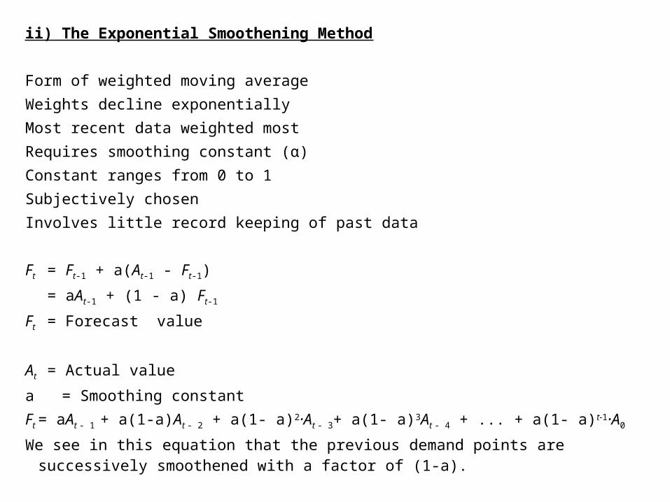
ii) The Exponential Smoothening Method Form of weighted moving averageWeights decline exponentiallyMost recent data weighted mostRequires smoothing constant (α)Constant ranges from 0 to 1Subjectively chosenInvolves little record keeping of past data Ft = Ft-1 + a(At-1 - Ft-1)
= aAt-1 + (1 - a) Ft-1
Ft = Forecast value
At = Actual value
a = Smoothing constantFt = aAt - 1 + a(1-a)At - 2 + a(1- a)2·At - 3+ a(1- a)3At - 4 + ... + a(1- a)t-1·A0
We see in this equation that the previous demand points are successively smoothened with a factor of (1-a).

Example:-You’re organizing a meeting. You want to forecast
attendance for year 2000 using exponential smoothing (a=.10). The 1995 (made in 1994) forecast was 175.Actual data: 1995 180
1996 1681997 1591998 1751999 190
Ft = Ft-1 + · (At-1 - Ft-1)

Time Actual Forecast, Ft (a=.10)
1995 180 175 (Given)
1996 168 175.00 + .10(180 - 175.00) = 175.50
1997 159 175.50 + .10(168 - 175.50) = 174.75
1998 175 174.75 + .10(159 - 174.75)= 173.18
1999 190 173.18 + .10(175 - 173.18) = 173.36
2000 173.36 + .10(190 - 173.36) = 175.02
By choosing a higher value of a , the model weights recent demand points more.Relation between the smoothing constant and response to error:Exponential smoothing is one of the most widely used techniques in forecasting.The quickness of the forecast adjustment to error is determined by the smoothing constant α.The closer the value of α to zero, the slower the forecast will respond to error- more smoothingThe closer the value of α to 1.00., the greater the forecast will respond to error -> less smoothing
iii) Linear RegressionThe simplest method to estimate the trend in a time series
is to treat the time periods as independent variables and the actual demand as a dependent variable. Using the standard method of least squares, it is possible to estimate the trend component.
Establishes a relationship between a dependent variable and one or more independent variables.
In simple linear regression analysis there is only one independent variable.
If the data is a time series, the independent variable is the time period.
The dependent variable is whatever we wish to forecast. (e.g. sales)

Delta Y
Delta X
a
b = Delta Y / Delta X = Slope
Example: b= ..0 means that for
every one unit increase in X , ..0
unit will increase in Y

Y = a + b X
Y = dependent variable (example: Company Sales)X = independent variable (example: time periods, sales of other related company) a = Y-axis interceptb = Slope of regression line = delta Y/ delta X
Constants a and b: The constants a and b are computed using the following equations:
22 XnX
YXnXYb
XbYa
Once the a and b values are computed, a future value of X (time, or sales of other elated product) can be entered into the regression equation and a corresponding value of Y (the forecast) can be calculated.
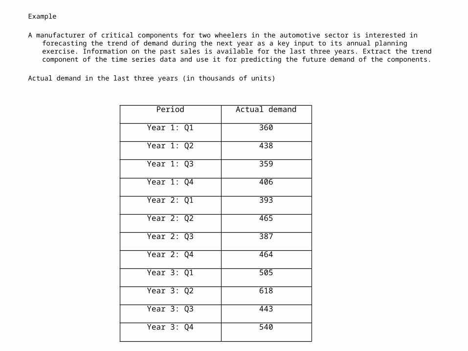
Example A manufacturer of critical components for two wheelers in the automotive sector is interested in forecasting the trend of demand
during the next year as a key input to its annual planning exercise. Information on the past sales is available for the last three years. Extract the trend component of the time series data and use it for predicting the future demand of the components.
Actual demand in the last three years (in thousands of units)
Period Actual demand
Year 1: Q1 360
Year 1: Q2 438
Year 1: Q3 359
Year 1: Q4 406
Year 2: Q1 393
Year 2: Q2 465
Year 2: Q3 387
Year 2: Q4 464
Year 3: Q1 505
Year 3: Q2 618
Year 3: Q3 443
Year 3: Q4 540

Solution
The model for forecasting using linear trend is denoted byY=a+ bX
From the above table, we compute the following:
X = 78/12=6.50
Y =5379/12=448.25
Computations for trend extraction using the method of least squares
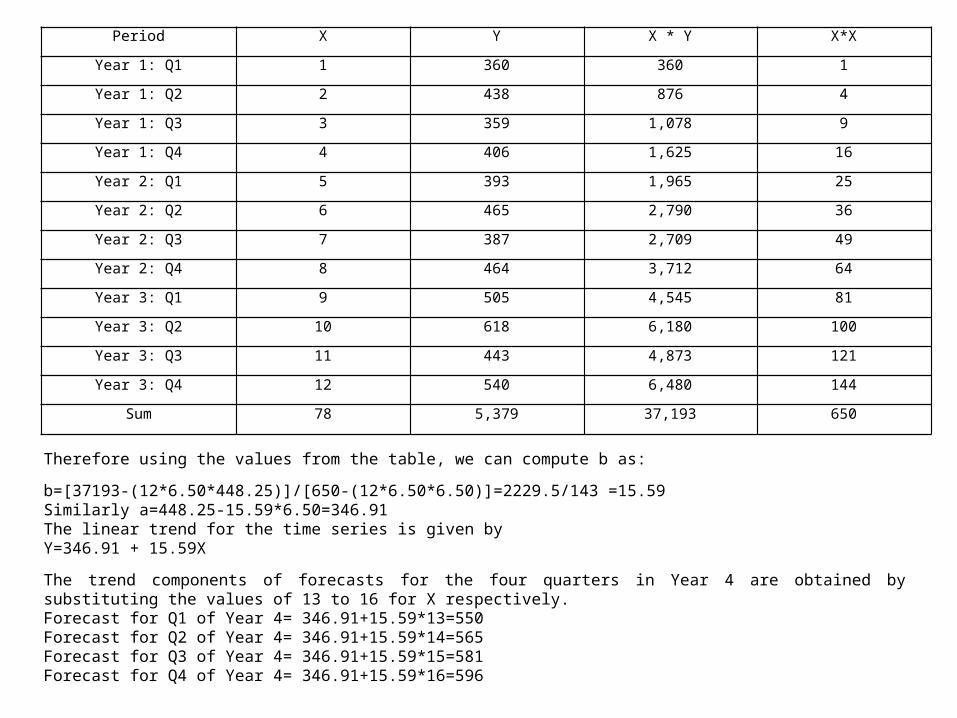
Period X Y X * Y X*X
Year 1: Q1 1 360 360 1
Year 1: Q2 2 438 876 4
Year 1: Q3 3 359 1,078 9
Year 1: Q4 4 406 1,625 16
Year 2: Q1 5 393 1,965 25
Year 2: Q2 6 465 2,790 36
Year 2: Q3 7 387 2,709 49
Year 2: Q4 8 464 3,712 64
Year 3: Q1 9 505 4,545 81
Year 3: Q2 10 618 6,180 100
Year 3: Q3 11 443 4,873 121
Year 3: Q4 12 540 6,480 144
Sum 78 5,379 37,193 650
Therefore using the values from the table, we can compute b as:
b=[37193-(12*6.50*448.25)]/[650-(12*6.50*6.50)]=2229.5/143 =15.59Similarly a=448.25-15.59*6.50=346.91The linear trend for the time series is given byY=346.91 + 15.59X
The trend components of forecasts for the four quarters in Year 4 are obtained by substituting the values of 13 to 16 for X respectively.Forecast for Q1 of Year 4= 346.91+15.59*13=550Forecast for Q2 of Year 4= 346.91+15.59*14=565Forecast for Q3 of Year 4= 346.91+15.59*15=581Forecast for Q4 of Year 4= 346.91+15.59*16=596


