Forecasting Hurricane Intensity: Lessons from

Application of the Coupled Hurricane Intensity Prediction

System (CHIPS)

Coupled Model DesignCoupled Model Design

Atmospheric Component: (from Emanuel, 1995)– Gradient and hydrostatic balance– Potential radius coordinates give very fine (~ 1 km)

resolution in eyewall– Interior structure constrained by assumption of moist

adiabatic lapse rates on angular momentum surfaces– Axisymmetric– Entropy defined in PBL and at single level in middle

troposphere– Convection based on boundary layer quasi-equilibrium

postulate– Surface fluxes by conventional aerodynamic formulae– Thermodynamic inputs: Environmental potential

intensity and storm-induced SST anomalies

Ocean Component:((Schade, L.R., 1997: A physical interpreatation of SST-feedback.

Preprints of the 22nd Conf. on Hurr. Trop. Meteor., Amer. Meteor. Soc., Boston, pgs. 439-440.)

• Mixing by bulk-Richardson number closure• Mixed-layer current driven by hurricane model

surface wind

Ocean columns integrated only Along predicted storm track.Predicted storm center SST anomaly used for input to ALLatmospheric points.

Data Inputs:–Weekly updated potential intensity (1 X 1 degree)–Official track forecast and storm history (NHC & JTWC)–Monthly climatological ocean mixed layer depths (1 X 1 degree)–Monthly climatological sub-mixed layer thermal stratification (1 X 1 degree)–Bathymetry (1/4 X 1/4 degree)

Initialization:

• Synthetic, warm core vortex specified at beginning of track

• Radial eddy flux of entropy at middle levels adjusted so as to match storm intensity to date

• This matching procedure effectively initializes middle tropospheric humidity as well as balanced flow

Comparison with same atmospheric model coupled to 3-D ocean model; idealized runs:

Full model (black), string model (red)

Mixed layer depth and currents

SST Change

Landfall Algorithm:

• Enthalpy exchange coefficient decreases linearly with land elevation, reaching zero when h = 40 m

• This accounts in a crude way for heat fluxes from low-lying, swampy or marshy terrain

Real-Time Forecasts Posted athttp://wind.mit.edu/~emanuel/storm.html

2002 Atlantic Intensity ErrorsOverall Forecast Performance:

12 14 16 18 20 22 2410

20

30

40

50

60

70M

axim

um s

urfa

ce w

ind

spee

d (m

/s)

Gert, 1999

September

ObservedModel Initialization period

Hurricane Gert occurred in a low-shear environmentand moved over an ocean close to its climatologicalmean state.

Same simulation, but with fixed SST:

Sensitivity to initial intensity error and length of matching period:

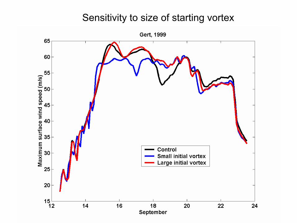
Sensitivity to size of starting vortex

Model performs poorly when substantial shear is present, as in Chantal, 2001:

16 17 18 19 20 21 22 23 240

10

20

30

40

50

60

70

August

Max

imum

sur

face

win

d sp

eed

(m s

-1)

Chantal, 2001

Best trackModel

Initialization period

16 17 18 19 20 21 22 23 240

2

4

6

8

10

12

August

Shea

r (m

s-1

)Chantal, 2001

850 – 200 hPa environmental shear:

Add “ventilation” term to model equationgoverning middle level θe. Coefficientdetermined by matching model to long

record of observations:

( )0e

e et

θθ θ

∂= − −

∂… V

2 2V Vmax shear=V

Result:

But model sensitive to shear: This shows the results of varyingShear magnitude by +/- 5 kts and +/- 10 kts:

Presence of shear also makes model sensitive to initial conditions.Here the initial intensity is varied by +/- 3 m/s and +/- 6 m/s:

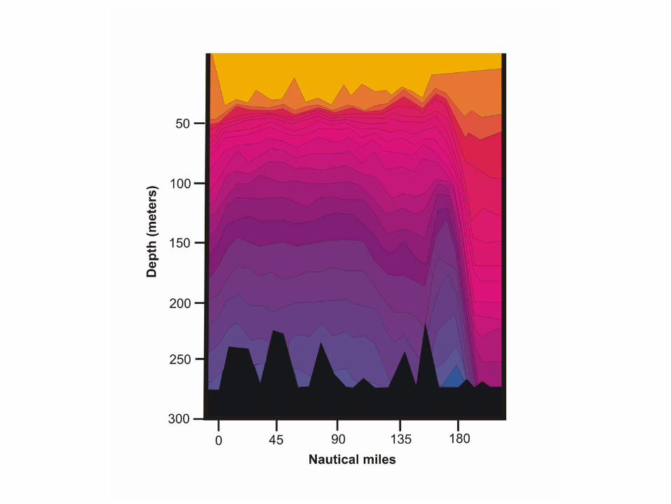
Some storms are influenced by upper ocean anomalies from monthly climatology. An example is that of Typhoon Maemi of 2003, which passed over a warm eddy in the western North Pacific:

Typhoon Maemi, 2003

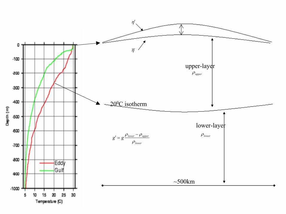
upper-layer

lower-layer

lower

upperlowerggρ

ρρ −=′

200C isotherm

upperρ

lowerρ

η′

η

~500km

Standard Simulation:

Using Sea Surface Altimetry to Estimate Upper Ocean Thermal Structure:

This shows model hindcasts with and without the ocean eddy,as estimated from sea surface altimetry data:

As TCs approach shore, shoaling water isolates surface mixed layer... surface cooling ceases.

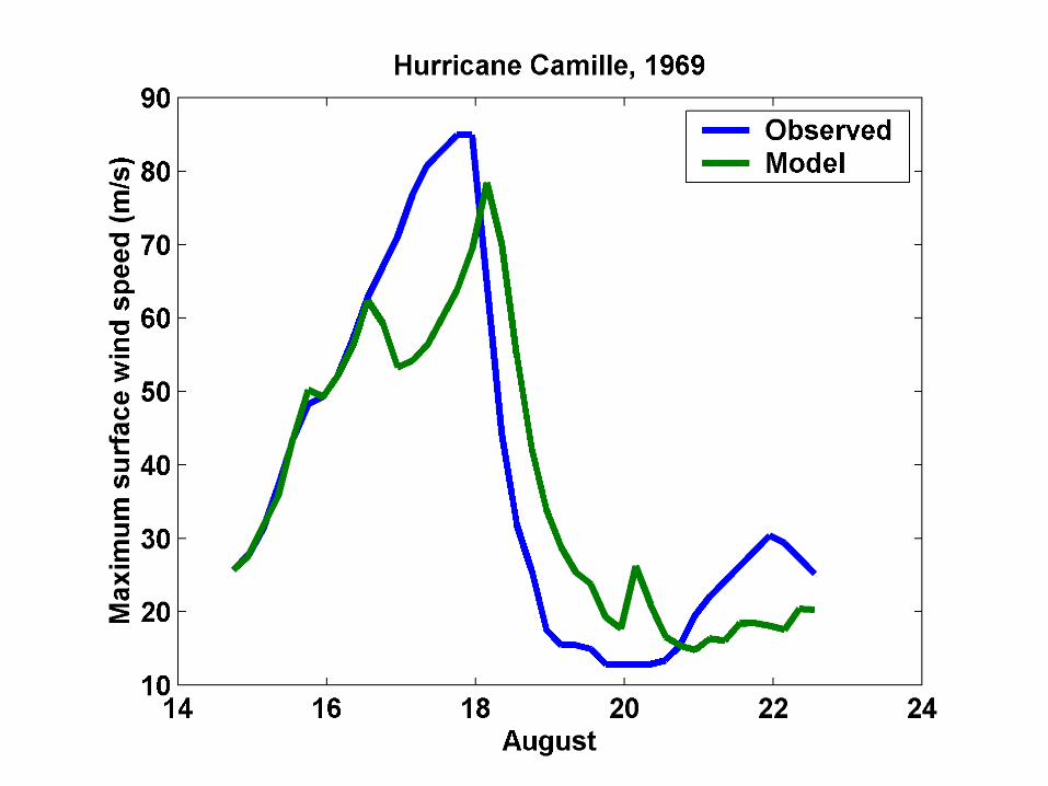
A good simulation of Camille can only be obtained by assuming thatit traveled right up the axis of the Loop Current:

Mitch was also influenced by an ocean eddy. The red curve used TOPEXaltimetry modified by de-aliasing the estimated peak amplitude:

Effect of standing water can be seen in these idealizedsimulations of storm landfall over dry land and overswamps with indicated depths of standing water:

Hurricane Andrew, with and without the effect of the Everglades,as represented by a elevation-dependent heat exchange coefficient:

Some storms may have large internal fluctuations (e.g. Allen). CHIPS may predict the existence of these, but not their phase:

Concentric eyewalls in Hurricane Gilbert, 1988 (from Black and Willoughby, Mon. Wea. Rev., 1992)

Solid: Beginning of fllight; Dashed: End of flight; Dotted: Change/6hr

Environmental factors critical to intensity prediction:

• Potential intensity along track• Upper ocean thermal structure• Environmental wind shear• Bathymetry• Land surface characteristics

Major sources of uncertainty:

• Uncertain forecasts of vertical shear• Shear reduces predictability• Little real-time knowledge of upper

ocean thermal structure• Low predictability of internal variability

Hurricanes and Climate

80 82 84 86 88 90 92 94150

160

170

180

190

200

210

220

230

240

Sea Surface Temperature (F)

Max

imum

Win

d Sp

eed

(MPH

)

0 2 4 6 8 10 1210

20

30

40

50

60

70

Time (days)

Max

imum

sur

face

win

d sp

eed

(m/s

)

ANDREW,1992

Control 2 X CO2

Empirical Index:

5

33 23

210 1 0.1 ,50 70

VpotI V

shearη

−= +H

1)850 ( ,hPa absolute vorticity sη −≡

1( ),V Potential wind speed mspot−≡

600 (%),mb relative humidity≡H1( ).

850 250V msshear

−≡ −V V

Atlantic

Western North Pacific

Paleotempestology

barrier beach

backbarrier marshlagoon

barrier beach

backbarrier marsh lagoon

a)

b)

Donnelly – Figure 2

upland

upland

flood tidal deltaterminal lobes

overwash fan

overwash fan

fine sand

mud withS. alterniflora

salt marsh peat

Dep

th (c

m)

0

50

100

150

200

250

300

350

WB2WB1 WB3

Whale Beach

??

1962 nor’easter

late 1700s or early 1800sprobably 1821 Hurricane

1278-1434 A.D.

pre-1932

(560 +50)1301-1370 A.D.1376-1434 A.D.

(680 +30)1278-1319 A.D.1353-1389 A.D.

Jeffrey Donnelly, WHOI

Beach DepositsNott and Hayne, 2001

250 750 1250 1750 2250 27500

1

2

3

4

5

6

7

Years before present

Num

ber o

f eve

nts

Lake Inwash DepositsNoren et al., 2002

Core stratigraphies

Sedimentation event histogram

GISP2 sea salt

GISP2 non-sea salt

Hummocky Cross-StratificationDuke, 1985

Brandt and Elias, 1989

Do tropical cyclones play a role in the climate system?

••The case for tropical cyclone control The case for tropical cyclone control of the thermohaline circulationof the thermohaline circulation

••Feedback of tropical cyclone activity Feedback of tropical cyclone activity on climateon climate

Tropical Cyclone-Climate Feedback

• Sensitive dependence of tropical cyclone frequency and intensity on tropical SSTs

+• Dependence of tropical SSTs on global

tropical cyclone activity

= Tropical thermostat

Ocean Feedback

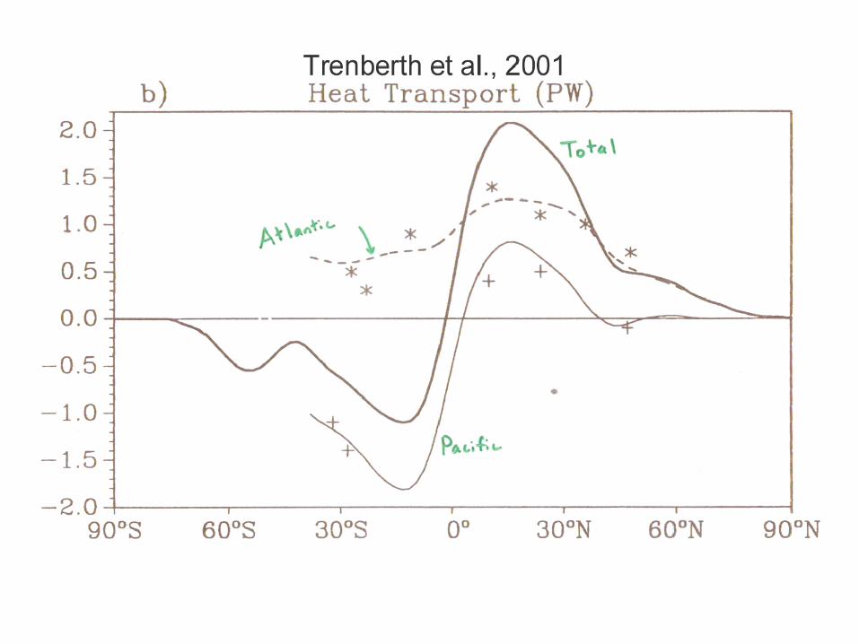
Ocean Thermohaline Circulation

Heat Transport by Oceans and Atmosphere

A hot plate is brought in contact with the left half of the surface of a swimming pool of cold water. Heat diffuses downward and the warm water begins to rise. The strength of the circulation is controlled in part by the rate of heat diffusion. In the real world, this rate is very, very small.

Adding a stirring rod to this picture greatly enhances the circulation by mixing the warm water to greater depth and bringing more cold water in contact with the plate. The strength of the lateral heat flux is proportional to the 2/3 power of the power put into the stirring, and the 2/3 power of the temperature of the plate.

Coupled Ocean-Atmosphere model run for67 of the 83 tropical cyclones that occurredin calendar year 1996

Accumulated TC-induced ocean heatingdivided by 366 days

Result:

Net column-integrated heating of oceaninduced by global tropical cyclone activity:

( ) 151.4 0.7 10 W± ×

Veronique Bugnion used an ocean model to calculate the sensitivity of the total poleward heat flux by the world oceans to the strength and distribution of vertical mixing. This sensitivity, shown here, is concentrated in the Tropics, where hurricanes occur.

These diagrams show the currents generated by a very localized source of vertical mixing at 20o N and 25o E. The upper diagram shows the currents near the top of the ocean, while the bottom diagram show currents closer to the bottom. Note in particular the strong northward flow of warm water along the western boundary of the ocean, near the surface. These plots have been generated using a complex ocean model set in a simple rectangular basin.

Courtesy of Jeff Scott

Implications for Climate:2

3Poleward Heat Flux FP∼

3F PI∼

3P PI∼

5Poleward Heat Flux PI→ ∼May be conservative, in view of Nolan’s results

This plot shows a measure of El Niño/La Niña (green) and a measure of the power put into the far western Pacific Ocean by tropical cyclones (blue). The blue curve has been shifted rightward by two years on this graph. There is the suggestion that powerful cyclones in the western Pacific can trigger El Niño/La Niña cycles.