30
By Srikavya Ravi teja Arun Nayak Karthik Amit Nayak
| Date post: | 15-Jul-2015 |
| Category: |
Data & Analytics |
| Upload: | srikavya-chowdary |
| View: | 347 times |
| Download: | 1 times |
BySrikavyaRavi teja
Arun Nayak Karthik
Amit Nayak

Forecasting lays a ground for reducing the risk in all decision making because many of the decisions need to be made under uncertainty.
In business applications, forecasting serves as a starting point of major decisions in finance, marketing, productions, and purchasing.
Method or technique for estimating many future aspects of a business or other operation.
It is used in the practice of customer demand planning in every day business forecasting for manufacturing companies.
There are three types of forecasting 1.Qualitative or Judgmental methods 2.Extrapolative or Time series methods 3.Causal or Explanatory methods

A time series is a sequence of data points, measured typically at successive points in time spaced at uniform time intervals.
Time series forecasting is the use of a model to predict future values based on previously observed values.
In this measurements are taken at successive points or over successive periods.

Time-Series
Cyclical Component
Random Component
Trend Component
Seasonal Component
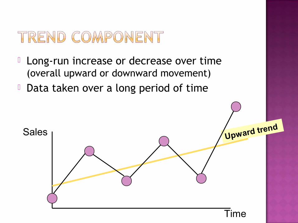
Long-run increase or decrease over time (overall upward or downward movement)
Data taken over a long period of time
Upward trendSales
Time

Trend can be upward or downward Trend can be linear or non-linear
Downward linear trend
Sales
Time Upward nonlinear trend
Sales
Time
(continued)
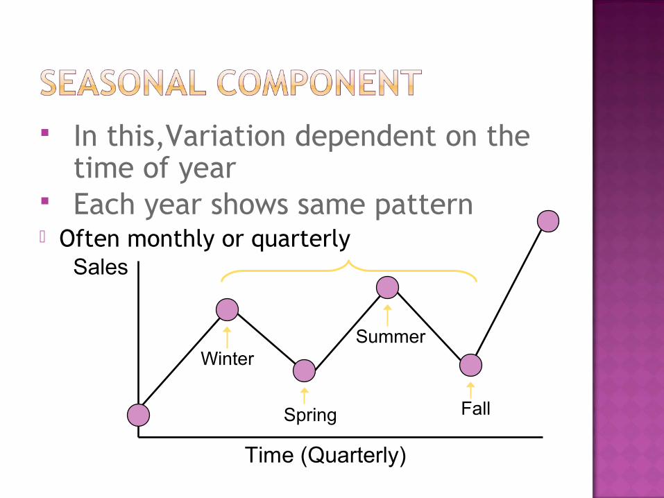
In this,Variation dependent on the time of year
Each year shows same pattern Often monthly or quarterly
Sales
Time (Quarterly)
Winter
Spring
Summer
Fall

Up & down movement repeating over long time frame
Regularly occur but may vary in length Each year does not show same pattern
Sales1 Cycle
Year
Unpredictable, random, “residual” fluctuations
Due to random variations of Nature Accidents or unusual events
“Noise” in the time series

Moving Average Method - average of demands occurring in several of the most recent periods.
Weighted Moving Average - allows for varying weighting of old demands.
Exponential Smoothing – exponentially decreases the weighting of old demands.
Linear method

The Simple Moving Average smooth past data by arithmetically averaging over a specified period and projecting forward in time. This is normally considered a smoothing algorithm and has poor forecasting results in most cases.
A moving average is commonly used with time series data to smooth out short-term fluctuations and highlight longer-term trends or cycles.
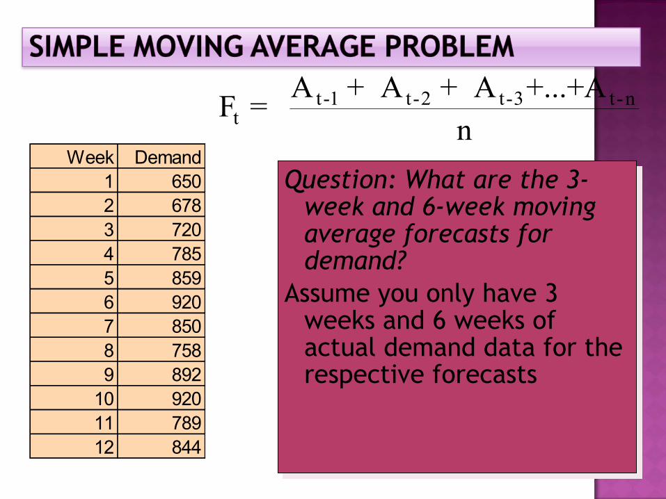
Question: What are the 3-week and 6-week moving average forecasts for demand?
Assume you only have 3 weeks and 6 weeks of actual demand data for the respective forecasts
Question: What are the 3-week and 6-week moving average forecasts for demand?
Assume you only have 3 weeks and 6 weeks of actual demand data for the respective forecasts
Week Demand1 6502 6783 7204 7855 8596 9207 8508 7589 892
10 92011 78912 844
F = A + A + A +...+A
ntt-1 t-2 t-3 t-n
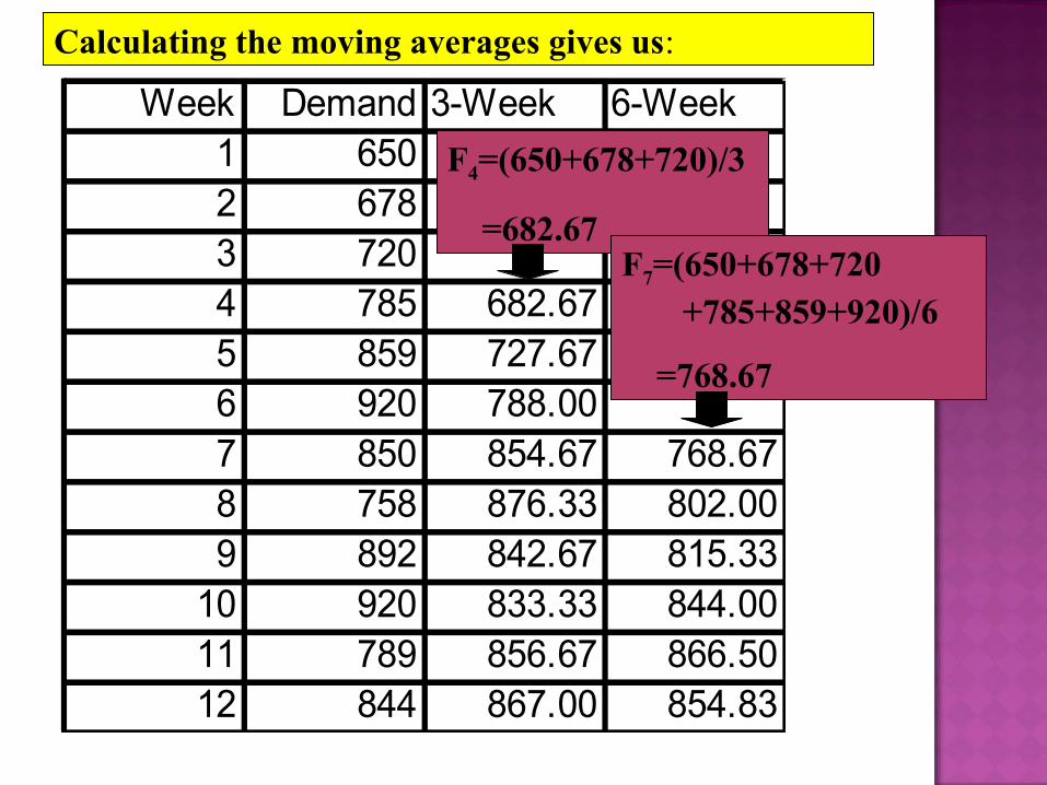
Week Demand 3-Week 6-Week1 6502 6783 7204 785 682.675 859 727.676 920 788.007 850 854.67 768.678 758 876.33 802.009 892 842.67 815.33
10 920 833.33 844.0011 789 856.67 866.5012 844 867.00 854.83
F4=(650+678+720)/3
=682.67F7=(650+678+720 +785+859+920)/6
=768.67
Calculating the moving averages gives us:
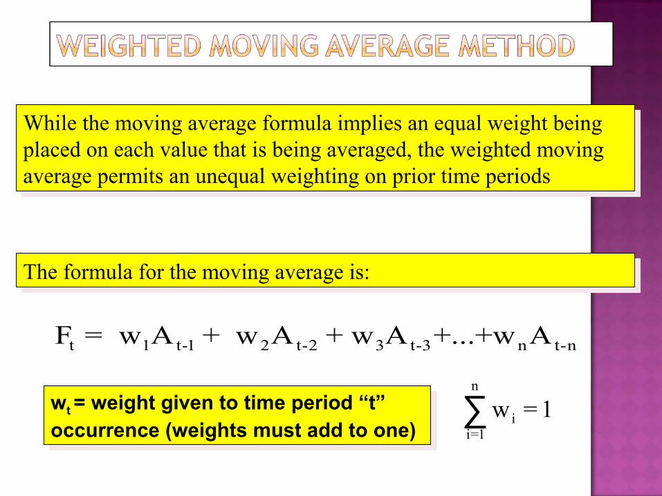
F = w A + w A + w A +...+w At 1 t-1 2 t-2 3 t-3 n t-n
w = 1ii=1
n
∑
While the moving average formula implies an equal weight being placed on each value that is being averaged, the weighted moving average permits an unequal weighting on prior time periods
While the moving average formula implies an equal weight being placed on each value that is being averaged, the weighted moving average permits an unequal weighting on prior time periods
wt = weight given to time period “t” occurrence (weights must add to one)
wt = weight given to time period “t” occurrence (weights must add to one)
The formula for the moving average is:The formula for the moving average is:

Weights: t-1 .5t-2 .3t-3 .2
Week Demand1 6502 6783 7204
Question: Given the weekly demand and weights, what is the forecast for the 4th period or Week 4?
Question: Given the weekly demand and weights, what is the forecast for the 4th period or Week 4?
Note that the weights place more emphasis on the most recent data, that is time period “t-1”
Note that the weights place more emphasis on the most recent data, that is time period “t-1”
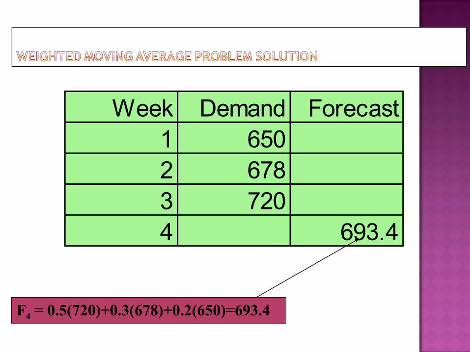
Week Demand Forecast1 6502 6783 7204 693.4
F4 = 0.5(720)+0.3(678)+0.2(650)=693.4

Drawback of previous models is carrying large amount of Data.As new data is added to this method, oldest observation is dropped and the new forecast is calculated. In many applications the most recent occurrences are more indicative of the future than those in the more distant past.If this premise is valid then Exponential smoothing may be the most logical method to use.Most used and widely used in retail firms, wholesale companies and service agencies.

Exponential smoothing is a technique that can be applied to time series data, either to produce smoothed data for presentation, or to make forecasts. Exponential smoothing methods give larger weights to more recent observations, and the weights decrease exponentially as the observations become more distant.

Premise: The most recent observations might have the highest predictive value
Therefore, we should give more weight to the more recent time periods when forecasting
Ft = Ft-1 + α(At-1 - Ft-1)Ft = Ft-1 + α(At-1 - Ft-1)
constant smoothing Alpha
period epast t tim in the occurance ActualA
period past time 1in alueForecast vF
period t timecoming for the lueForcast vaF
:Where
1-t
1-t
t
===
=
α
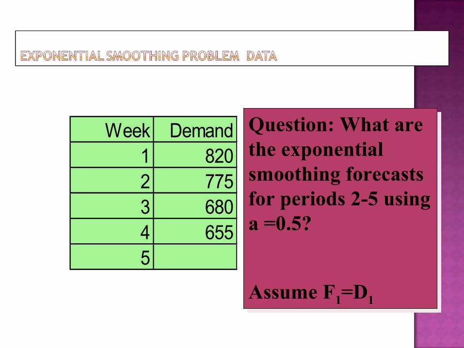
Question: What are the exponential smoothing forecasts for periods 2-5 using a =0.5?
Assume F1=D1
Question: What are the exponential smoothing forecasts for periods 2-5 using a =0.5?
Assume F1=D1
Week Demand1 8202 7753 6804 6555

Week Demand 0.51 820 820.002 775 820.003 680 797.504 655 738.755 696.88
F1=820+(0.5)(820-820)=820 F3=820+(0.5)(775-820)=797.75
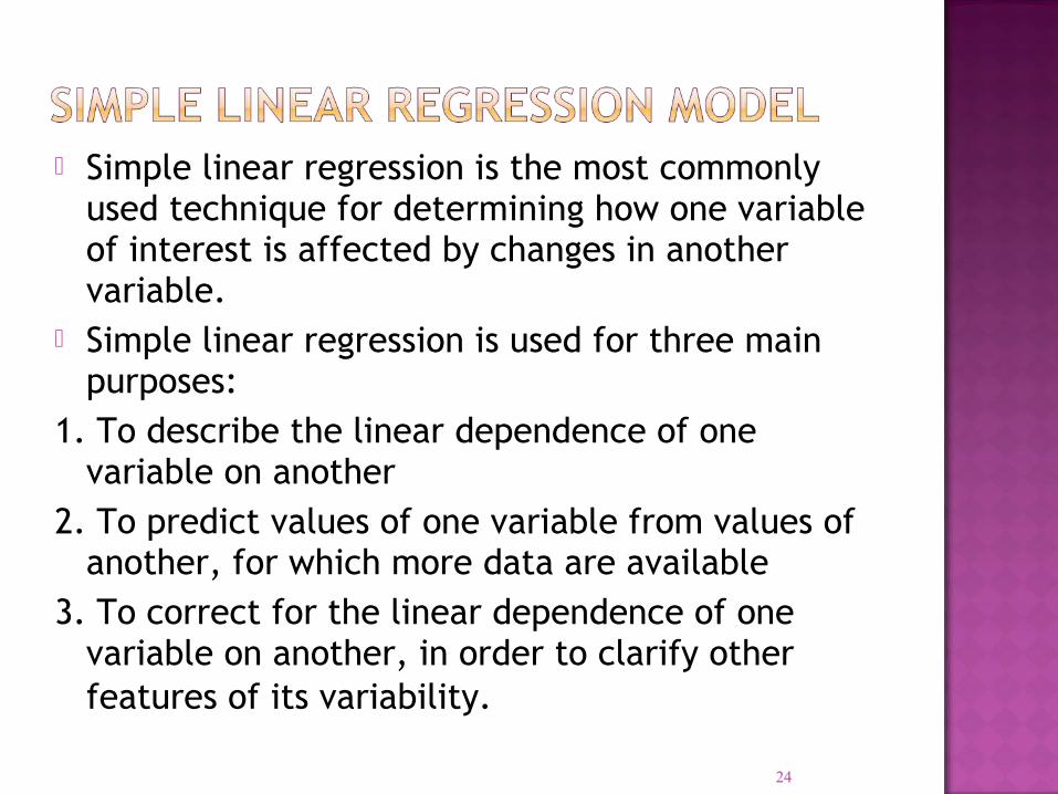
Simple linear regression is the most commonly used technique for determining how one variable of interest is affected by changes in another variable.
Simple linear regression is used for three main purposes:
1. To describe the linear dependence of one variable on another
2. To predict values of one variable from values of another, for which more data are available
3. To correct for the linear dependence of one variable on another, in order to clarify other features of its variability.
24
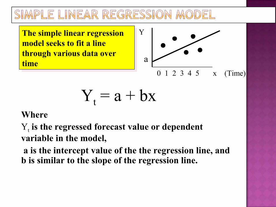
Yt = a + bx
0 1 2 3 4 5 x (Time)
YThe simple linear regression model seeks to fit a line through various data over time
The simple linear regression model seeks to fit a line through various data over time a
Where Yt is the regressed forecast value or dependent variable in the model, a is the intercept value of the the regression line, and b is similar to the slope of the regression line.

a = y- bx
b =xy - n(y)(x)
x - n(x2 2
∑
∑ )
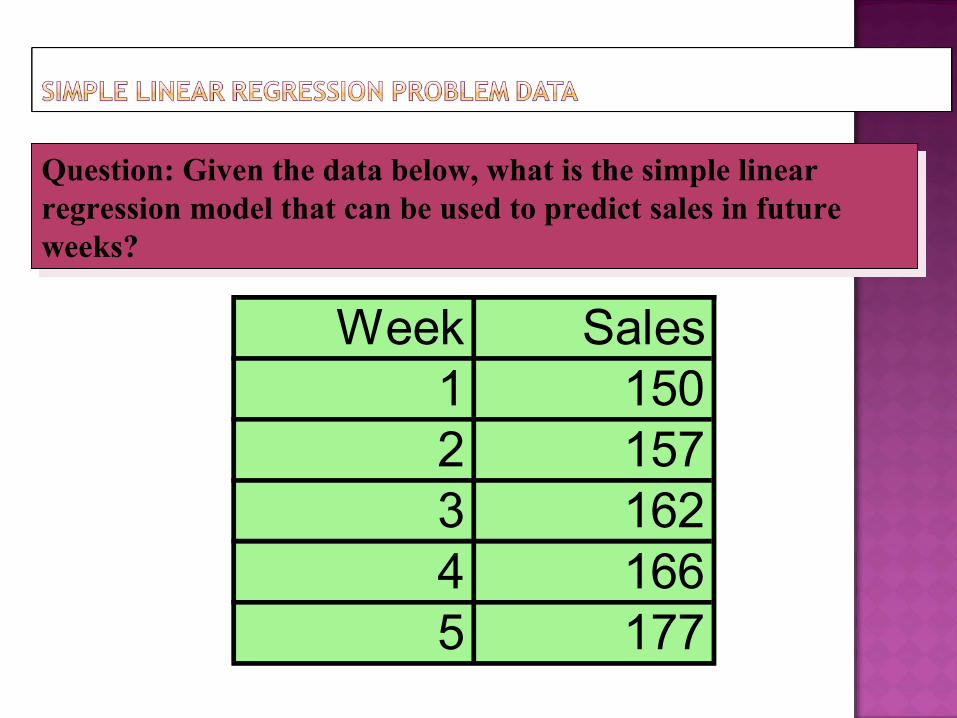
Week Sales1 1502 1573 1624 1665 177
Question: Given the data below, what is the simple linear regression model that can be used to predict sales in future weeks?
Question: Given the data below, what is the simple linear regression model that can be used to predict sales in future weeks?
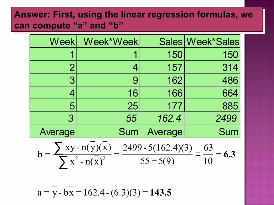
Week Week*Week Sales Week*Sales1 1 150 1502 4 157 3143 9 162 4864 16 166 6645 25 177 8853 55 162.4 2499
Average Sum Average Sum
b =xy - n(y)(x)
x - n(x=
2499 - 5(162.4)(3)=
a = y - bx = 162.4 - (6.3)(3) =
2 2
∑∑ −
=) ( )55 5 9
63
106.3
143.5
Answer: First, using the linear regression formulas, we can compute “a” and “b”
Answer: First, using the linear regression formulas, we can compute “a” and “b”

Yt = 143.5 + 6.3x
180
Period
135140145150155160165170175
1 2 3 4 5
Sal
es
Sales
Forecast
The resulting regression model is:
Now if we plot the regression generated forecasts against the actual sales we obtain the following chart:

30


