2006 VOLUME 130M O N T H L Y W E A T H E R R E V I E W

q 2002 American Meteorological Society

Forecasting Skill Limits of Nested, Limited-Area Models: A Perfect-Model Approach

RAMON DE ELIA AND RENE LAPRISE

Departement des Sciences de la Terre et de l’Atmosphere, Universite du Quebec a Montreal, Montreal, Quebec, Canada

BERTRAND DENIS

Recherche en Prevision Numerique, Meteorological Service of Canada, Dorval, Quebec, Canada

(Manuscript received 16 July 2001, in final form 12 December 2001)

ABSTRACT

The fundamental hypothesis underlying the use of limited-area models (LAMs) is their ability to generatemeaningful small-scale features from low-resolution information, provided as initial conditions and at theirlateral boundaries by a model or by objective analyses. This hypothesis has never been seriously challenged inspite of some reservations expressed by the scientific community. In order to study this hypothesis, a perfect-model approach is followed. A high-resolution large-domain LAM driven by global analyses is used to generatea ‘‘reference run.’’ These fields are filtered afterward to remove small scales in order to mimic a low-resolutionrun. The same high-resolution LAM, but in a small-domain grid, is nested within these filtered fields and runfor several days. Comparison of both runs over the same region allows for the estimation of the ability of theLAM to regenerate the removed small scales.

Results show that the small-domain LAM recreates the right amount of small-scale variability but is incapableof reproducing it with the precision required by a root-mean-square (rms) measure of error. Some success isattained, however, during the first hours of integration. This suggests that LAMs are not very efficient in accuratelydownscaling information, even in a perfect-model context. On the other hand, when the initial conditions usedin the small-domain LAM include the small-scale features that are still absent in the lateral boundary conditions,results improve dramatically. This suggests that lack of high-resolution information in the boundary conditionshas a small impact on the performance.

Results of this study also show that predictability timescales of different wavelengths exhibit a behavior similarto those of a global autonomous model.

1. Introduction

Limited-area models (LAMs) are powerful tools forpredicting and studying weather patterns and have beenused by the scientific community for some time (seereferences provided by White et al. 1999). Over the lastdecade there has been an explosion in the use of thesemodels in a variety of research and operational appli-cations because of their ability to perform, in local high-resolution studies, without the enormous computationalcost of a global model at the same resolution. In somecases the objective is to run simulations or forecasts ata higher resolution than that given in the initial andboundary conditions, with the expectation that the in-crease in model resolution, which sometimes implies animprovement in both the dynamics and physics, en-hances the quality of the simulation. A fundamental

Corresponding author address: Ramon de Elıa, Departement desSciences de la Terre et de l’Atmosphere, Universite du Quebec aMontreal, B.P. 8888, Succ. Centre-ville, Montreal, QC H3C 3P8,Canada.E-mail: relia@sca.uqam.ca

hypothesis underlying the use of LAMs is, hence, theirability to generate meaningful small-scale features thatare absent in the initial and boundary conditions. Inshort, this implies that small-scale features are generatedby the model independently of the small-scale featurespresent in reality but absent in the initial and lateralboundary conditions. This independence may be attri-buted to the ability of the larger scales to regenerate thesmaller scales (as if they remain in a ‘‘latent’’ state), ormay mean that surface forcings (e.g., mountains, lakes,etc.) play an important role in their excitation.

In spite of the importance of the aforementioned hy-pothesis, a surprisingly small number of studies havebeen devoted to proving it. However, a number of stud-ies carried out within the last 15 years have producedresults that are relevant for this topic, especially thoserelated to predictability in LAMs. Anthes et al. (1985)proposed two opposite points of view: a pessimistic one,which argues using turbulence theory that predictabilityin smaller scales is more limited than it is in larger scalesdue to the shorter overturning time; and an optimisticone, which suggests that relevant mesoscale meteoro-logical phenomena are highly organized (far from tur-

AUGUST 2002 2007D E E L I A E T A L .

bulent) and therefore exhibit long-term predictability.Several researchers performed experiments that wereinterpreted as favorable to the optimistic approach. An-thes et al. (1985) reported that predictability in nestedLAMs is different from that of global forecast models.Using ensemble integrations of a LAM nested with ob-jective analyses at the lateral boundaries, they showedthat errors in the initial conditions do not grow beyondan asymptotic value that is much smaller than the valueexpected for the case of total loss of correlation (aswould the case with a global model). This result sug-gested the possibility that LAMs possess some kind of‘‘extended predictability.’’ Errico and Baumhefner(1987) expanded this work to study individual scalesby means of spectral analyses, and confirmed the resultsfor each spatial scale.

Shortly after, this particular characteristic of LAMswas widely acknowledged. Vukicevic and Paegle (1989)mention in their introduction that, ‘‘All the studies ofpredictability which uses local models show decay orno growth of the domain integrated root mean squarederror throughout the forecast.’’ Further research in thisarea by Anthes et al. (1989), Warner et al. (1989), Vuk-icevic and Errico (1990), Berri and Peagle (1990), Zengand Pielke (1993), Giorgi et al. (1993), Jones et al.(1995), Giorgi and Marinucci (1996), and Peagle et al.(1997) confirmed previous results and described the sen-sitivity of the results to different parameters such asdomain size, topography, etc. The influence of errors inthe boundary conditions was also studied and was foundto be much more important than sensitivity to initialconditions. In addition, Peagle et al. (1997) found that,without the existence of the driving boundaries, errorsin small scales tend to grow, confirming that extendedpredictability is not a property of the scales understudy—usually meso-a—but is a consequence of nest-ing. However, Boer (1994) did find an increase in pre-dictability of small scales in a global model, attributablemostly to the stationarity of mountain-induced distur-bances.

Notwithstanding the evidence gathered by years ofresearch, part of the scientific community remains un-convinced of the capability of nested LAMs to repro-duce small scales faithfully. In a report of the WorkingGroup on Numerical Experiment (WGNE 1999), it isargued that questions concerning this point remain tobe answered. A review of the articles already mentionedin this introduction lends support to this point of view,since authors found some results that did not allow fora simple interpretation. In one of the experiments ofAnthes et al. (1985), errors in some variables grow lin-early for 72 h. Since several sources of error were pre-sent in this experiment, subsequent experiments con-centrate on simpler, better-defined problems that showedno error growth. However, the first result is not ex-plained in light of the others. In Vukicevic and Paegle(1989) part of the article is devoted to a theoretical studyin which it is shown, using a simple barotropic model,

that short Rossby–Haurwitz (R–H) waves have less pre-dictability than long ones. They concluded that, ‘‘Thedifference between R–H wavenumber 2 and R–H wave-number 4 results suggests that the boundary constraintmay not be enough to suppress the error growth if theflow contains smaller scale waves.’’ Van Tuyl and Errico(1989) found, using a mesoscale model, that the self-interaction of large scales does not contribute signifi-cantly to small scales, which suggests that the recreationof small scales may not be controlled by the large scales.In Berri and Peagle (1990), experiments with a small-domain high-resolution model display sensitivity to ini-tial conditions, while experiments with the same modelat 10 times lower resolution and larger domain do not.

It is interesting to note that in most articles concerningthis topic, the problem of the effect of one-way nestingis not thoroughly analyzed. In few articles (e.g., Antheset al. 1985) there is a comparison between the outputfields of the nested model and the driving fields. Ingeneral, several runs of the LAM are performed for thesame boundary conditions but for slightly different ini-tial conditions, and the outputs of these runs are thenused for predictability studies. Unfortunately, this wide-spread procedure leaves the study of the nesting per seout of the question. For this reason, the informationprovided by such experiments does not shed much lighton the question of the LAMs ability to recreate small-scale information; it only describes the internal vari-ability of the model.

The WGNE (1999) in its annual report suggested toconstruct an experiment to study the downscaling inLAMs. Following this suggestion, Laprise et al. (2000)presented results of such an experiment using a LAM-generated dataset to drive the same LAM but in a smallerdomain. In order to replicate the effect of low-resolutionnesting data, fields provided by the driving model to beused as lateral boundary and initial conditions weresmoothed. The authors found ‘‘no evidence for extendedpredictability of scales that are not forced through thelateral boundary conditions,’’ challenging most of theresults presented to date. On the other hand Denis et al.(2001), following a similar approach, studied the abilityof a regional climate model to reproduce the high-res-olution variability that had been removed form its lateralboundary conditions, and found that the model repro-duced rather well the original small-scale information;in this case, the model was not asked to simulate thedata in a deterministic day-by-day basis but to simulateits climate statistics. The present study continues themethodology followed by the last two previously men-tioned articles, but concentrates on the short-term evo-lution of weather systems, as in Laprise et al. (2000).

As discussed by Giorgi and Bi (2000) when studyingsensitivity experiments with LAMs, the presence of in-ternal variability should be taken into consideration. Forthis reason, a predictability study precedes the analysisof the downscaling abilities of the model. Each one isdiscussed using a different set of experiments with a

2008 VOLUME 130M O N T H L Y W E A T H E R R E V I E W

FIG. 1. Schematic of the experimental design. (left) Low-resolution global analyses are used to drive the LAM in the largedomain. Fields obtained by this simulation are then used to drive the LAM in a small domain (located within the largedomain), after being filtered to mimic low resolution conditions. (right) After a time T of integration, fields from both runscan be compared for the overlapping region to evaluate small-scale regeneration.

perfect-model approach, in which a LAM is nested withdata generated by the same model, but in a larger do-main. Section 2 describes the experimental design andthe characteristics of the LAM, while section 3 presentsthe description and results of predictability and down-scaling experiments. A summary and conclusions aregiven in section 4.

2. The experimental framework

The original proposal in the WGNE (1999) reportsuggested the approach of the ‘‘identical twin’’ para-digm, with ‘‘a very high resolution global model as acontrol and a simulation with a LAM identical to thatof the global model.’’ Such an experiment would permita comparison between the two models inside the re-gional grid and, hence, an assessment of the ability ofthe regional model to replicate the global model. Manyother experiments can also be performed with this setup.For example, by smoothing the global fields, a realisticrepresentation of the data sparseness may be achieved.

By driving the LAM with this filtered data, it wouldthen be possible to evaluate the ability of the arrange-ment to re-create the small-scale features present in theglobal model prior to filtering.

There are many factors that make such an experimentimpractical, however, especially the computational cost.Furthermore, it may be considered unnecessary sincethe only area of interest in the global grid is the sur-roundings of the regional grid. A more pragmatic ap-proach could be to run a single regional model on twodifferent domain sizes: a large one that plays the roleof the global model, and a small one located inside theprevious one. The large-size domain LAM can be nestedwith objective analyses for a given period of time, andafter a spinup time it will develop its own variability.The second domain, small enough to be far from theboundaries, can be driven by the large one, using exactlythe same model and the same grid spacing. Figure 1 isa schematic of the experimental design. On the left, thetime evolution of the large-domain LAM driven by low-resolution global analyses is represented. On the right,

AUGUST 2002 2009D E E L I A E T A L .

TABLE 1. Parameters in model simulations.

Parameter Value

Time stepGrid-point spacingLarge domainSmall domainLarge domain driven bySmall domain driven by

15 min45 km (true at 608N)196 3 196 grid points 3 18 levels100 3 100 grid points 3 18 levels12-h NCEP analyses3-h large-domain simulation

FIG. 2. Large and small integration domains.

the time evolution of the small-domain LAM, driven byfiltered large-domain LAM-produced fields, is shown.Since both the small-domain and the large-domain runhave the same grid spacing, a comparison at all resolvedscales is possible.

The LAM used in the following experiments is theCanadian Regional Climate Model (CRCM) describedin Caya and Laprise (1999). It consists of a limited-areagridpoint nonhydrostatic model that uses a three-time-level semi-Lagrangian semi-implicit time-marchingscheme. The nesting technique is one way, and wasdeveloped by Robert and Yakimiw (1986) and tested byYakimiw and Robert (1990), based on the work of Da-vies and Turner (1977). The nesting zone region is ninepoints wide along the lateral boundaries, in which thehorizontal velocity components are relaxed toward thosefrom the driving model. The grid uses a polar-stereo-graphic projection true at 608 latitude, and a Gal-Chenvertical coordinate. A complete description of the dy-namical formulation of the CRCM, including the nestingimplementation, can be found in Bergeron et al. (1994)and Laprise et al. (1997). The physical parameterizationis described in Caya and Laprise (1999), although thepresent version includes the moist convective schemeof Kain and Fritsch (1990). The time evolution of thesea surface temperature (SST) was imposed by linearlyinterpolating monthly mean climatological data. Table1 describes some important parameters used in the sim-ulations of both the large and small domains. The choiceof updating the boundary information of the small-do-main LAM every 3 h came as a compromise betweenthe necessity of not affecting the short waves enteringthe domain, and the intention to resemble operationalsetups. With this value, in a weather system with a speedof 10 m s21, wavelengths shorter than 100 km are af-fected, while the grid spacing allows for wavelengthslonger than 90 km. Figure 2 shows the layout and lo-cation of the domains. The ratio between domain sizesfollows the recommendations of Giorgi and Mearns(1999), who suggest that in order to study an area ofinterest of length scale L, the boundaries should be re-moved by a distance L/2. Considering the small domainas the area of interest with length scale L, the largedomain should then have a length scale 2L.

A 35-day integration of the CRCM is performed overthe large domain, nested with National Centers for En-vironmental Prediction (NCEP) objective analyses start-ing 27 January 1993. This high-resolution simulation

(‘‘reference run’’ hereafter) becomes the ‘‘truth’’ withwhich other runs will be compared. Several experimentswith the small domain are performed in which somevariation is introduced either in the boundary conditionsor in the initial conditions. For all cases, 24 4-day in-tegrations of the LAM are performed in the small do-main starting on 1 February and then at successive 24-h intervals. Figure 3 describes the integration schedule.In order to achieve statistical stability, results are esti-mated using the 24 runs of the small-domain CRCM.In this way, for example, an n-h integration ensembleaverage implies the average over 24 different n-h in-tegrations, beginning 1 day apart.

3. Results

In order to gain further physical insights a scale anal-ysis was performed on the obtained fields, and this con-stitutes an important part of this study. Difficulties inproducing meaningful spectra from nonglobal gridshave forced researchers to seek reliable algorithms (e.g.,Errico 1985). In this work, results obtained using thediscrete cosine transform (DCT) are presented (Deniset al. 2001, 2002). Computations were also performedusing the algorithm of Errico (1985), and these providedcomparable results.

The subregion of the nested LAM computational do-main over which the spectral analysis must be per-formed is also a delicate matter. If the entire compu-tational domain is used, the influence of lateral boundarynesting information will contaminate the results. If thearea chosen to carry the spectral analysis is very farfrom the boundaries, the amount of data is reduced con-siderably, resulting in poor spectra. Experiments showed

2010 VOLUME 130M O N T H L Y W E A T H E R R E V I E W

FIG. 3. Schematic of the models’ integration schedule. The reference run is represented by the upper and lower long horizontal lines. Shorthorizontal lines depict the beginning and ending of small-domain LAM runs. The dashed line indicates the cases considered for a study ofaverage error after 24 h of integration. Small squares inside dotted boxes signal the individual comparisons.

that by avoiding the nesting zone, variability inside thesubregion was almost uniform. Hence, results are basedon the analysis of a subregion of 80 3 80 within the100 3 100 small domain.

Results presented below will concentrate on the anal-ysis of the vorticity fields at 850 hPa. Other levels andother variables were carefully inspected, and results didnot vary substantially. Nevertheless, certain advantagesin the selected field and level influenced our decision:(i) the vorticity spectra has considerable energy in thesmall scales, which permits clear visibility of small per-turbations and minimizes the error of the spectra esti-mation, as shown by Denis et al. (2002); (ii) the 850-hPa level is high enough not to be disrupted by topog-raphy, but low enough to display substantial energy inthe small scales. For purposes of illustration, other var-iables are also shown in some cases. It is worth men-tioning that by choosing a pressure level far from thesurface, the topographic effects are less noticeable. Thisimplies that results should be interpreted cautiously, notallowing a straightforward generalization to the surfacefields.

a. Predictability

Predictability was studied by performing model in-tegrations over the small domain without filtering thedriving data (from the large domain), but introducing asmall perturbation into the initial conditions. This was

done by interpolating the driving data from model Gal-Chen levels into pressure levels, and then back to modellevels. This procedures mimics, to some extent, theGCM–LAM mode of operation. As expected, inertio–gravity waves are generated in the first few time stepsbut disappear promptly. As Errico and Baumhefner(1987) explained, ‘‘the fastest gravity waves do notstrongly interact with the more slowly varying, andmore important synoptic systems. Therefore, they onlyweakly affect the solution differences of such systems.’’

Figure 4a shows a time sequence of the square rootof the average spectrum, for the difference between the850-hPa vorticity fields of the reference run and theperturbed simulations, normalized by the average vor-ticity spectrum of the reference run. This normalizedspectrum may be interpreted as the normalized root-mean-square (rms) difference between the fields as afunction of wavenumber. It can be seen that the growthis highly dependent on wavenumber, being very limitedfor small wavenumbers and almost reaching the criticalvalue associated with uncorrelated signals ( ) forÏ2large wavenumbers. This behavior, found in all studiedvariables (wind, temperature, geopotential, specific hu-midity, precipitation, and divergence), suggests the ex-istence of three different regimes: (i) synoptic-scale fea-tures that remain highly correlated after many hours ofintegration owing to forcing exerted by the lateralboundary conditions, (ii) mesoscale features that behaverandomly after less than 2 days because of inherent

AUGUST 2002 2011D E E L I A E T A L .

FIG. 4. Normalized RMS difference for the 850-hPa vorticity fields, between the reference run and the perturbed small-domain run. (a)The rms as a function of wavenumber for days 0–4; (b) the time evolution of four chosen wavelengths, as well as an example of the curvedefined in (1) fitting wavenumber k 5 20; (c) the asymptotic values obtained by fitting each wavenumber with (1); and (d) the values ofthe parameters t0 and t obtained by fitting the time evolution of the different wavenumbers with (1), the dashed line indicating a linear fit,for wavenumbers larger than k 5 4, with the slope value printed at the lower bottom right.

predictability limits, and (iii) an intermediate bandwhose properties seem to resist a simple interpretation.

The temporal evolution of selected wavenumbers isdisplayed in Fig. 4b. It shows that, although all wav-enumbers tend to reach different asymptotic values, eachscale possesses a particular timescale in which thesevalues are reached. The time evolution of the normalizedrms has been fit with a curve defined as

2t/tRMS 5 B 2 Ae , (1)where the parameter t is related with the timescale ofthe error growth and B is the asymptotic value to whichthe RMS converges after long integration times. Theparameter A can be better understood if expressed as A5 B exp (2t0/t), where t0 represents the time before t5 0 when the RMS for a given wavelength was iden-tically zero. Then (1) can be rewritten as

2012 VOLUME 130M O N T H L Y W E A T H E R R E V I E W

2(t 2 t )/t0RMS 5 B[1 2 e ]. (2)

The degree of freedom represented by t0 could havebeen removed, but exploration of results suggestedkeeping it. Since the size of errors at the initial time arescale dependent, there are regions of the spectrum inwhich RMS is already large at t 5 0 (see solid line inFig. 4a). The parameter t0 can be interpreted as theamount of time it should have taken a very small butfinite perturbation at a given wavenumber to reach theactual size of the perturbation present at time zero. Sincethis number is a function of the size of the initial per-turbation, we considerer it as physically unimportant.

Figure 4c shows the asymptotic value B obtained foreach wavenumber. The curve, as expected, resemblesthose observed in Fig. 4a after 4 days of integration.Figure 4d displays the obtained values of the timescalet as a function of wavenumber in a log–log diagram.The straight line fitted to wavenumbers larger than k 54 suggests that t can be expressed as

dt 5 ck , (3)

with a slope d 5 20.67. This power law was not specificto the vorticity at 850 hPa but was present in all thestudied variables and at all levels. As an additional ex-ample of this, the parameter t for temperature, geopo-tential, specific humidity (all of them at 850 hPa), and3-h precipitation are shown in Fig. 5. It can be seen thatfor temperature (Fig. 5a) and geopotential (Fig. 5b) re-sults are noisy for small wavelengths. This is due to thefact that variables that contain very little energy in theshortest wavelengths are sensitive to error in the spectralestimation, as discussed in Denis et al. (2002). Specifichumidity (Fig. 5c) and precipitation (Fig. 5d), with lesssteep spectra, display results very similar to that of vor-ticity (Fig. 4d).

Lorenz (1969) found that each scale of motion hasan intrinsic finite period of predictability; for a globalmodel it was shown that this limit varies inversely withwavenumber, which implies a relation t ; kd, with sloped 5 21. Since our experiment provided only one timeseries, the error in the estimation of d is unknown. How-ever, estimations using different periods of the time se-ries, as well as different variables, gave values differingby about 0.4. Because of the inaccuracy of this esti-mation it would be unrealistic to claim that this LAMexhibits a different behavior from the global model.However, results for all variables seem to suggest a slopeof d . 21, which may indicate a slower loss of pre-dictability. These results imply that sensitivity to initialconditions is present at all wavelengths.

This sensitivity, however, does not evolve toward atotal loss of correlation. Because of the information pro-vided at the lateral boundaries, differences asymptoteto values smaller than or equal to , with smallerÏ2values at large scales. A complete parameterization ofthe evolution of the normalized RMS according towavelength can be obtained by using (1), where the

parameter B can be approximated by fitting the curveobtained in Fig. 4c with the function used in (1), whilet can be expressed as in (3). In this way, the normalizedRMS can be approximated by

d2k/k 2t/ckRMS (k, t) 5 C(1 2 e )(1 2 e ), (4)

where C and k are obtained by fitting the curves asdescribed above. Results show that the asymptotic valuefor long periods of times and large wavenumbers, theparameter C, is always close to , as expected, butÏ2some small variations were found. Figure 6 depicts theparameterized normalized RMS for vorticity as a func-tion of wavenumber k and time t, which may be com-pared to the experimental data displayed in Fig. 4a.Although this curve has been obtained for vorticity at850 hPa, all variables analyzed (wind, temperature, geo-potential, specific humidity, precipitation, and diver-gence) display similar characteristics. This parametricrepresentation seems to summarize well the averageproperties of the normalized RMS as a function of wave-number and time. In fields with very steep spectra (e.g.,geopotential), the ‘‘deterministic’’ region predominates,resulting in low values for the total rms error. In noisierfields such as vorticity, the ‘‘turbulent’’ region has moreimportance, resulting in larger values for the total rms.

The shape of the curve presented in Fig. 6 shows thatone-way nesting mostly controls the error growth atlarge scales, despite the presence of all wavenumbersin the boundary conditions. This curve can be inter-preted as the highest level of accuracy that this modelcan achieve under this configuration and, therefore, isa landmark to be compared to in other experiments.

Results show that for the shorter scales the loss ofcorrelation is almost total. This seems to contradict theexperience of many forecasters who claim that the ex-istence of surface forcing enhances the predictability ofsmall scales, and which was confirmed more than adecade ago by Vukicevic and Errico (1990). In fact, tworeasons might help to make this effect unnoticeable here:(i) as is mentioned in the beginning of this section, thechosen level may not contain much information re-garding the surface forcing, and (ii) one distinctive fea-ture of the spectral analysis is that it gives integratedvalues over the entire domain, diluting the localizedeffects of the surface forcings (e.g., Appalachians, land–ocean contrast) with the surrounding homogeneity.

b. Downscaling ability

When small-scale information is absent in the bound-ary and initial conditions, the challenge to the LAM isto regenerate small scales that are similar to the originaldata. In order to perform these experiments, the refer-ence run was filtered and later used as the initial andboundary conditions for the small-domain LAM. Thesmoothing of data was performed with the same DCTspectral filtering mentioned in the beginning of section3 (see Fig. 8, where the responses for different cut fre-

AUGUST 2002 2013D E E L I A E T A L .

FIG. 5. Values of the parameters t0 and t obtained by fitting the time evolution of wavenumbers larger than k 5 4, as in Fig. 4d but for(a) temperature at 850 hPa, (b) geopotential at 850 hPa, (c) specific humidity at 850 hPa, and (d) 3-h precipitation.

quencies of the low-pass filter are displayed as solidlines). This particular shape of the filter was chosenbecause of its similarity to the way in which data fromlow-resolution global models project into LAMs: Sincenot all wavenumbers present in the sphere exist in theregional grid, the abrupt truncation of wavenumbers inthe global grid is reflected in a smoother way in theregional domain.

Several experiments with different cut frequencieswere performed. Table 2 lists the different cases, indi-cating the minimum resolved wavelength in kilometers

and grid points, the equivalent jump J between reso-lutions of the driving data and the LAM, and the equiv-alent resolution for a global model. Figure 7 shows anexample of data in the small domain before and afterfiltering for J8.

Before studying the rms differences between the fil-tered small-domain runs and the reference runs, an eval-uation of the variability created by the small-domainLAM is needed. For this purpose, it is useful to analyzethe evolution of the spectrum of the small-domain runnormalized by the reference run spectrum (average of

2014 VOLUME 130M O N T H L Y W E A T H E R R E V I E W

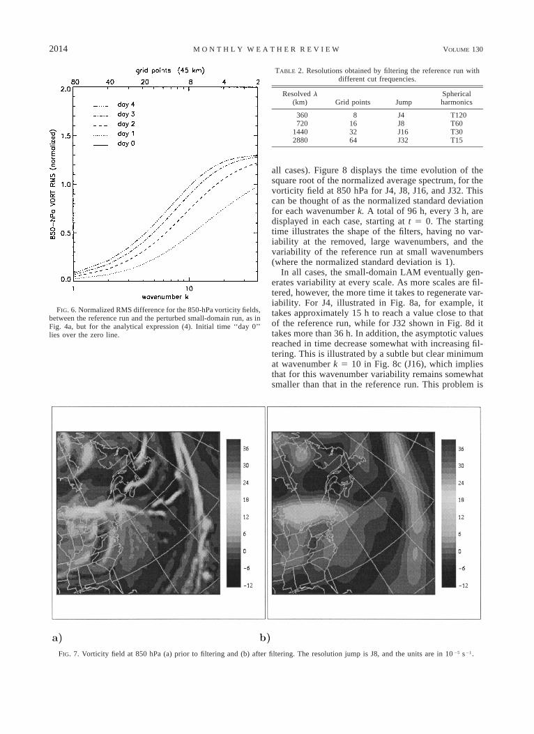
FIG. 6. Normalized RMS difference for the 850-hPa vorticity fields,between the reference run and the perturbed small-domain run, as inFig. 4a, but for the analytical expression (4). Initial time ‘‘day 0’’lies over the zero line.

TABLE 2. Resolutions obtained by filtering the reference run withdifferent cut frequencies.

Resolved l(km) Grid points Jump

Sphericalharmonics

360720

14402880

8163264

J4J8J16J32

T120T60T30T15

FIG. 7. Vorticity field at 850 hPa (a) prior to filtering and (b) after filtering. The resolution jump is J8, and the units are in 10 25 s21.

all cases). Figure 8 displays the time evolution of thesquare root of the normalized average spectrum, for thevorticity field at 850 hPa for J4, J8, J16, and J32. Thiscan be thought of as the normalized standard deviationfor each wavenumber k. A total of 96 h, every 3 h, aredisplayed in each case, starting at t 5 0. The startingtime illustrates the shape of the filters, having no var-iability at the removed, large wavenumbers, and thevariability of the reference run at small wavenumbers(where the normalized standard deviation is 1).

In all cases, the small-domain LAM eventually gen-erates variability at every scale. As more scales are fil-tered, however, the more time it takes to regenerate var-iability. For J4, illustrated in Fig. 8a, for example, ittakes approximately 15 h to reach a value close to thatof the reference run, while for J32 shown in Fig. 8d ittakes more than 36 h. In addition, the asymptotic valuesreached in time decrease somewhat with increasing fil-tering. This is illustrated by a subtle but clear minimumat wavenumber k 5 10 in Fig. 8c (J16), which impliesthat for this wavenumber variability remains somewhatsmaller than that in the reference run. This problem is

AUGUST 2002 2015D E E L I A E T A L .

FIG. 8. Normalized standard deviation of the 850-hPa vorticity field for all wavenumbers. Values are plotted every 3 h for (a) J4, (b) J8,(c) J16, and (d) J32. The initial time (first solid line starting from the bottom) illustrates the corresponding filter response.

even more evident in Fig. 8d (J32), where wavenumbersk 5 1 and k 5 2 were strongly affected by filtering.

It is interesting to note that, for a given filtering value,the variance in all wavenumbers that are absent in theinitial and lateral boundary conditions seems to growin time at the same rate. This is evinced by the fact that,for larger wavenumbers, the curves representing dif-ferent times are almost parallel horizontal straight lines.An estimation of the timescale of the downscaling pro-cess can be obtained by fitting the time evolution of thestandard deviation of the wavelengths affected by trun-

cation with (1) as was done for Fig. 4b. These fittingsshowed that the timescale t is weakly dependent onwavelength, and was found to be for all the studiedvariables: J4, t ; 6 h; J8, t ; 8 h; J16, t ; 12 h; andJ32, t ; 18 h. The values for J4 and J8 are smallerthan those of the predictability timescales depicted inFig. 4d, which shows variations between 10 and 40 hfor different wavelengths. This is a necessary result ifthe aim is to recreate the small scales before the internalvariability takes over.

The results presented above show that the one-way

2016 VOLUME 130M O N T H L Y W E A T H E R R E V I E W

FIG. 9. Normalized RMS difference for the 850-hPa vorticity fields as a function of wavenumber for days 0–4, as in Fig. 4a, but for (a)J4, (b) J8, (c) J16, and (d) J32.

nesting develops finescale features when nested withsufficiently high resolution in the initial and in the lateralboundary conditions. The almost exact reproduction ofthe variance of the reference run (ratio close to 1) canbe explained by the fact that both the reference run andthe filtered run use the same LAM and similar but dif-ferently truncated boundary conditions.

The evaluation of the forecasting skill requires morethan studying the ability to reproduce the right level ofvariability: the quality of the small scales generated alsoneeds to be studied. To study the accuracy of the re-

created small-scale features, we now examine the nor-malized RMS difference between the filtered small-do-main run and the reference run. Figure 9 shows thenormalized RMS difference as is defined for Fig. 4a butfor different resolution jumps in initial and lateralboundary conditions. The normalized RMS 5 1 for theremoved length scales at the initial time illustrates wellthe effect of filtering.

For nearly all scales error increases with time, al-though there is a narrow band of scales near the limitof filtering where the error decreases in time for a short

AUGUST 2002 2017D E E L I A E T A L .

FIG. 10. Time evolution of the normalized RMS difference for the 850-hPa vorticity fields for four chosen wavenumbers, as in Fig. 4b,but for (a) J4, (b) J8, (c) J16, and (d) J32.

period. After around 2 days of integration, values be-come nearly asymptotic, and by days 3 and 4 they seemalready quite stable. In comparison with Fig. 4a, thefour cases reach asymptotic values at a higher RMS,although cases J4 and J8 (panels a and b) appear to bequite similar. Figure 10 displays the temporal evolutionof four selected wavenumbers for each of the resolutionjumps shown in Fig. 9. In general it can be seen thatsome wavenumbers affected by filtering (e.g., k 5 10,in Figs. 10a and 10b) tend to diminish the normalizedRMS during the first hours of integration, and soon after

this a loss of precision takes over. The amount of timeit takes this minimum to be reached varies with caseand wavenumber, ranging from 6 h for k 5 10 in J4(Fig. 10a) to 24 h for k 5 5 in J16 (Fig. 10c).

Comparisons between Figs. 10 and 4b shed some lightregarding the behavior of the downscaling. As was notedin the previous section, the time evolutions displayedin Fig. 4b represent the landmark against which thequality of the downscaling should be compared. Theoptimal situation would have been a rapid reduction inthe RMS of those wavelengths affected by filtering, until

2018 VOLUME 130M O N T H L Y W E A T H E R R E V I E W

FIG. 11. Normalized RMS as a function of wavenumber for anaverage solid shift in a hypothetical field. Plotted lines illustrate val-ues for different distributions of shifts, having standard deviations S5 [0.5, 1.0, 1.5, 2.0, 2.5, 3.0] in gridpoint units.

loss of predictability brings up the RMS in a way similarto that in the slightly perturbed case of Fig. 4b. Resultsshow that the reduction of RMS in all cases shown inFig. 10 is not as fast and marked as might have beenexpected. For example, the lowest RMS value for k 510 in the case J4 (reached at 6 h, as shown in Fig. 10a)is 0.6, while at the same time and the same wavelengthfor the slightly perturbed experiment RMS 5 0.2 (Fig.4b). For shorter wavelengths the situation is even worse,as can be seen with k 5 20 in J8 case (Fig. 10b). Here,there is only a hint of a reduction of RMS at 6 h, andafterward this values increase monotonically (with theexception of a few minor oscillations that might be as-sociated with a daily wave).

Although it is difficult to evaluate the importance ofthe RMS reduction in the first hours of integration, thereis no doubt that some wavelengths do not show anyrelevant sign of reduction. These results suggest that thedownscailing is, from a deterministic point of view, notas efficient as had been hoped.

c. Interpreting the error

In order to evaluate the importance of the errors dis-played in Figs. 4a and 9 we propose two different butrelated ways of interpreting the results. The first methodconsists of a theoretical evaluation of the impact on therms of a solid shift of a field, while the second studiesthe effect of a temporal displacement with exact data.

1) SOLID SHIFT

Let us first consider a two-dimensional field f (x, y)that can be written as a Fourier series as

N

i2p (kx1ly)f (x, y) 5 Re A e , (5)O kl[ ]k,l50

where Akl is the amplitude; k and l are wavenumbers inthe x and y directions, respectively; and i the imaginaryunit. A solid shift in the field can be represented as f (x2 Dx, y 2 Dy), where Dx and Dy are the displacementin the x and y directions, respectively. Then the differ-ence f (x, y) 2 f (x 2 Dx, y 2 Dy) can be written as

f (x, y) 2 f (x 2 Dx, y 2 Dy)

N

i2p (kDx1lDy) i2p (kx1ly)5 Re A [1 2 e ]e . (6)O kl5 6k,l50

After rearranging the terms it can be shown that thespectral variance Skl of this difference can be ex-pressed as

2 i2p (kDx1lDy) 2S 5 | A | | 1 2 e | .kl kl (7)

Defining SM as the average spectrum with M 2 5 k2 1l2 we then obtain

M1S 5 S 2 2OM kÏM 2kM k51

M225 A [1 2 cos2p (kDx 1 lDy)]. (8)2 2O kÏM 2kM k51

Since the normalized 5 SM/A2, by assuming for2RMSM

simplicity that the amplitudes Akl are identical, that thedisplacement is in only one direction, and using theidentity

M sin2p (M 1 1/2)Dx 1cos ka 5 2 , (9)O

2 sin2pMDx/2 2k51

we obtain

1 sin2p (M 1 1/2)Dx2RMS 5 2 1 2 2 1 . (10)M 5 6[ ]2M sin2pMDx/2

We can estimate an average value of for several2RMSM

cases assuming, for example, that the shift Dx followsa normal distribution N0,S with nil average value (nosystematic shift) and a variance S 2. Then,

`

2 2RMS 5 RMS (x)N (x) dx. (11)M E M 0,S

2`

Figure 11 displays a numerical solution of the previousintegral for S 5 [0.5, 1.0, 1.5, 2.0, 2.5] in gridpointunits. The curves represent the average normalized RMSfor solid displacements Dx of the field, having a normal

AUGUST 2002 2019D E E L I A E T A L .

FIG. 12. Normalized RMS as a function of wavenumber for anaverage temporal shift. Plotted lines illustrate values for differentshifts Dt 5 [30, 60, 90, 120, 150, 180] min.

distribution with zero mean displacement and standarddeviation S. Since the mean displacement is nil, bothpositive and negative directions are allowed.

This diagram may be thought of as the effect of phaseerror of weather systems on the RMS for each wave-length. As expected, an error in the position of theweather system affects more strongly the shorter wave-lengths. It can be seen that for S 5 0.5 (i.e., a standarddeviation of half grid point in the distribution of spatialshifts), the rms error obtained is similar to that of 1 dayof integration in the LAM for k 5 1 and k 5 2 (seeFig. 4a). For larger wavenumbers, it is clear that a 1-day integration produces errors closer to S 5 1.0. Forlonger integration periods, it can be seen that for smallwavenumbers, rms errors are comparable to those pro-duced by S , 1, while for intermediate wavenumbers(e.g., k 5 10), rms errors correspond to larger valuesof S.

Larger error for the intermediate wavenumbers maycome from error in the relative position of short waveswith respect to the weather system, or in their intensity.It is important to note that since error asymptotes nearnormalized RMS 5 , a comparison of large RMSÏ2values gives little information regarding overall fielddifferences.

2) TEMPORAL DISPLACEMENT

In order to complement the previous study of solidspatial displacement, a temporal shift is also performed.The rms difference between successive fields of thesame time series can also be interpreted as the rms errorof a delayed perfect forecast. The normalized RMS dif-ference between successive fields Dt apart for the vor-ticity field at 850 hPa is therefore computed. Averagesof 4 days’ worth of data, 30 min apart, are displayedin Fig. 12 for different values of Dt 5 [30, 60, 90, 120,150, 180] min.

It is interesting to notice that a 60-min delay of aperfect forecast (Fig. 12) seems to have a similar effecton all wavenumbers as an integration of a LAM during1 day (Fig. 4a). It can be seen that a 90-min delay ofa perfect forecast generates an error in the long wavessimilar to that of many days of integration in the pre-dictability study of Fig. 4a. A longer time delay is re-quired to generate an error in intermediate wavenumbers(e.g., wavenumber k 5 7), comparable to that of a fewdays of integration: to reach a comparable rms error tothat found in the predictability study, the perfect forecastshould be delayed by around 180 min. Large waven-umbers reach saturation error in both cases, makingcomparison unprofitable.

Results from both the solid and temporal shift suggestthat an important part of the error in small scales mightbe explained as a small error in the phase of the weathersystems, and visual inspection confirmed that this wasthe case in several instances. This happens in spite ofthe fact that the long waves are imposed at the bound-

aries, and that both simulations use the same LAM. Itis also clear from these computations that the rms is avery sensitive error measurement tool and that resultsshould be interpreted under this perspective.

One issue that surfaces in this analysis is that therequirement that short wavelengths be ‘‘in phase’’ im-poses restrictions beyond what is necessary for a veryacceptable weather forecast (e.g., a delay of less than30 min). What is implicit in this discussion is that bygoing into smaller scales the forecaster not only desiresa good spatial resolution of weather phenomena but alsoa higher accuracy in the timing. This may not neces-sarily be the case since even if the future allows for agrid spacing of 40 m, the forecaster will not be con-cerned with delays of the order of the 2 s. Continualimprovement in spatial resolution does not change thefact that human activities remain mostly the same.

d. Experiments with high-resolution initial conditionsand low-resolution boundary conditions

In some cases, a region of dense data is surroundedby an area of relatively sparse data (e.g., continentalUnited States). When a LAM is utilized over this kindof region, the initial conditions include small-scale fea-tures while the lateral boundary conditions that drivethe model have coarser resolution.

This particular distribution of data was representedby running a set of experiments identical to the onespresented in Table 2, with the exception that in this case

2020 VOLUME 130M O N T H L Y W E A T H E R R E V I E W

FIG. 13. As in Figs. 4b and 10 but for the case where only lateral boundary conditions are filtered (initial conditions remain unfiltered).

the initial conditions were not filtered, thus maintainingthe quality of the reference run at initial time. Figure13 shows the time evolution for selected wavenumbersfor the same resolution jumps in lateral boundary con-ditions as were shown in Fig. 10. Comparisons betweenthe respective panels indicate that cases with similarresolution in the boundaries (e.g., Fig. 10a and Fig. 13a)reach the same asymptotic values, suggesting, as shownby previous studies, that the rms difference becomesindependent of the initial conditions after a certain pe-riod. On the other hand, for the first 24 h the RMSgrowth for J4 and J8 (Figs. 13a and 13b, respectively)

does not differ much from the case with high-resolutioninformation in both initial and boundary conditions (Fig.4b). These experiments show the very important impactof the initial conditions on the rms difference in the firsthours of integration. This is quite striking for the caseswith smaller resolution jumps (J4 and J8), in which asimilar growth rate of the rms difference with respectto the high-resolution driven model is found. This seemsto suggest that if boundaries are set, as is usually rec-ommended, far from the region of interest, the qualityof the simulation is rather insensitive to the resolutionof the driving data. This can be interpreted in two ways,

AUGUST 2002 2021D E E L I A E T A L .

as good news highlighting the remarkable job of a LAMgiven the right initial conditions, and as a warning thatincreasing resolution in the lateral boundary driving datamay only have a very limited impact on the rms error.

In this experiment the model was not required todownscale information but to generate a reliable sim-ulation from filtered lateral boundary conditions. Thesuccess may be due to either the ability to maintain theevolution of small-scale features, despite the degradedlateral boundary conditions, or that the rate of degra-dation due to the internal variability is faster than thecorruption introduced by the lateral boundary condi-tions. In either case the results seem to support the ra-tionale of limited-area modeling provided that goodquality high-resolution initial and good quality low-res-olution lateral boundary conditions are provided.

4. Concluding remarks

The ability of LAMs to recreate small-scale featuresthat were absent in the initial and/or the lateral boundaryconditions was studied. For this purpose, a regionalmodel (CRCM) was used to perform several runs of thesame resolution in two different domains: one large,nested with NCEP analyses, and one a small, locatedwithin the large one and nested with the values obtainedby this large-domain simulation. This experimental set-up allowed us to perform different studies in a perfect-model environment, thus concentrating on the nestingeffect rather than on intrinsic model errors. Hence ourresults can be interpreted as the upper limit of skillachievable with an imperfect LAM nested with imper-fect initial and lateral boundary conditions. Results pre-sented here are essentially based in the analysis of vor-ticity at 850 hPa, but results in other variables showedsimilar characteristics.

Our predictability studies suggest that the initialgrowth rates in nested LAMs may not differ substan-tially from those of global models. In global models,however, the asymptotic limit of the normalized RMSdifference reaches , while for LAMs, the asymptoticÏ2value reached by the normalized RMS is less than orequal to , varying with length scale. For small scalesÏ2the asymptotic values is close to , while for largeÏ2scales the asymptotic value is much smaller than ,Ï2illustrating the concept of ‘‘extended predictability’’first introduced by Anthes et al. (1985). Results showthat one-way nesting mostly controls the error growthat large scales, even when all wavenumbers are presentin the boundary conditions. No signal was found tosuggest that surface forcings extend the predictability,although it is discussed that the chosen height level, theselected region, and the characteristics of the spectralanalysis do not highlight it.

When the initial and lateral boundary conditions ofthe LAM are degraded by smoothing or filtering, theLAM is able to regenerate the variability lost by filter-ing. The recreated small scales, however, differ from

the original ones as revealed by the rms study. Differ-ences with the reference run grow with time in mostwavenumbers, with the exception of a narrow band closeto the truncation wavenumber whose RMS decreasesduring the first hours. This decrease in RMS is not verypronounced, and after some time, all wavenumbersreach asymptotic RMS values that are higher than initialvalues. The importance of the decrease in RMS seemsdifficult to assess, and may require a different approachto the data analysis. However, it is clear that from adeterministic point of view the downscaling is not veryefficient.

When the initial conditions contain high-resolutioninformation and the boundary conditions are filtered,the normalized RMS difference evolves similarly to theone produced by the unfiltered case. This suggests thatthe quality of the simulation is rather insensitive to theresolution of the driving data, which implies on onehand that the rationale behind the LAMs is sound, andon the other the inefficiency of increasing the resolutionin the lateral boundary conditions as a means of im-proving the simulation quality.

An important point is suggested by the study in sec-tion 3c, which compares the effect of both a solid dis-placement of the weather system and a delayed perfectforecast on the rms. These comparisons suggest thatphase delays of the order of some hours may producethe same error as that produced by a lack of predict-ability after a few days of integration. This comparisonraises the question of the fairness of demanding pre-cision in time proportional to wavelength, which is animplicit assumption in our scale analysis.

It may be of interest to repeat these experiments bynesting the model through the nudging of large scales(von Storch et al. 2000; Biner et al. 2000) and therebyeliminating completely the error in the large scales. Withthis approach, error in the smaller scales could not comefrom phase errors induced by slight errors at largerscales.

Throughout the text it has been mentioned that theuse of an rms error measure imposes restrictions on thegeneralizability of the conclusions. Of no less impor-tance is the difficulty of this or any other score skill tosummarize the predominant features of a given exper-iment. This is why the visual inspection of meteoro-logical fields has been carried out carefully. In the pre-dictability and in the J4 and J8 downscaling experi-ments, fields with sharp spectra (e.g., geopotential) lookalmost identical, with some differences in phase or in-tensity when the field includes an intense weather sys-tem. Variables that allowed for small-scale inspectionbecause of their spectral characteristics (e.g., vorticity)show that small scales associated with weather systemsare normally recreated but sometimes at the wrong placeand with a different shape.

High-resolution LAMs have been used for many dif-ferent applications. If the application aims to increasethe accuracy of the prediction in intensity and phase at

2022 VOLUME 130M O N T H L Y W E A T H E R R E V I E W

a given point, results presented here suggest there is alimited gain by running a high-resolution model becauseof the short predictability limit of small scales and theinefficiency of the downscaling phenomena. Some ad-ditional research, however, is needed to estimate thesignificance of the gain in the first hours of integration,which may be of importance according to the subjectiveexperience of many forecasters. As White et al. (1999)put it: ‘‘numerical products available from recentlyemerging mesoscale model guidance provide valuableinsight, but still lack the specificity to justify point-wisewarnings’’.

The results of Denis et al. (2001), which employeda similar methodology to the one presented here but forclimate timescales, do lend confidence as to the abilityof high-resolution LAMs to gain accuracy in a statisticalsense.

Caution must be exerted in generalizing these ten-tative conclusions because too little is known about theirsensitivity to factors not considered here, such as do-main size, grid spacing, nesting frequency, dynamics,physics, nesting method, season, geographical location,topography, score skill, etc. These results, however, con-stitute a warning against overenthusiastic expectationsregarding mesoscale predictions with LAMs.

Acknowledgments. We are very grateful to the sci-entific and technical staff of the Canadian Regional Cli-mate Model Group (CRCM) at UQAM for their unlim-ited accessibility, and to Claude Desrochers for main-taining an efficient computing environment for theCRCM group. This work has been financially supportedby Canadian NSERC, funding from the U.S. Departmentof Energy Climate Change Prediction Program (CCPP),and the UQAM regional climate modeling group. Wegratefully acknowledge the Meteorological Service ofCanada for granting an education leave to the third au-thor during this study and for providing access to itscomputer facilities.

REFERENCES

Anthes, R. A., Y. H. Kuo, D. P. Baumhefner, R. M. Errico, and T.W. Bettge, 1985: Predictability of mesoscale motions. Advancesin Geophysics, Vol. 288, Academic Press, 159–202.

——, ——, S. Low-Nam, and T. W. Bettge, 1989: Estimation of skilland uncertainty in regional numerical models. Quart. J. Roy.Meteor. Soc., 115, 763–806.

Bergeron, G., R. Laprise, and D. Caya, 1994: Formulation of theMesoscale Compressible Community (MC2) model. CooperativeCentre for Research in Mesometeorology Internal Rep., 165 pp.[Available from Dr. D. Caya, Groupe des Sciences del’Atmosphere, Departement des Sciences de la Terre et del’Atmosphere, Universite du Quebec a Montreal, B.P. 8888,Succ. Centre-ville., Montreal, QC H3C 3P8, Canada.]

Berri, G. J., and J. Paegle, 1990: Sensitivity of local predictions toinitial conditions. J. Appl. Meteor., 29, 256–267.

Biner, S., D. Caya, R. Laprise, and L. Spacek, 2000: Nesting of RCMsby imposing large scales. Research Activities in Atmosphericand Oceanic Modeling, WMO Rep. 30, CAS/JSC Working

Group on Numerical Experimentation (WGNE), WMO/TD-987,7.3–7.4.

Boer, G. J., 1994: Predictability regimes in atmospheric flow. Mon.Wea. Rev., 122, 2285–2295.

Caya, D., and R. Laprise, 1999: A semi-implicit semi-Lagrangianregional climate model: The Canadian RCM. Mon. Wea. Rev.,127, 341–362.

Davies, H. C., and R. E. Turner, 1977: Updating prediction modelsby dynamical relaxation: An examination of the technique.Quart. J. Roy. Meteor. Soc., 103, 225–245.

Denis, B., R. Laprise, J. Cote, and D. Caya, 2001: Downscaling abilityof one-way nested regional climate models: The big-brother ex-periment. Climate Dyn., 18, 627–646.

——, J. Cote, and R. Laprise, 2002: Spectral decomposition of two-dimensional atmospheric fields on limited-area domains usingthe discrete cosine transform (DCT). Mon. Wea. Rev., 130, 1812–1829.

Errico, R., 1985: Spectra computed from a limited area grid. Mon.Wea. Rev., 113, 1554–1562.

——, and D. Baumhefner, 1987: Predictability experiments using ahigh-resolution, limited-area model. Mon. Wea. Rev., 115, 488–504.

Giorgi, F., and M. R. Marinucci, 1996: An investigation of the sen-sitivity of simulated precipitation to model resolution and itsimplications for climate studies. Mon. Wea. Rev., 124, 148–166.

——, and L. Mearns, 1999: Introduction to special section: Regionalclimate modeling revisited. J. Geophys. Res., 104, 6335–6352.

——, and X. Bi, 2000: A study of internal variability of a regionalclimate model. J. Geophys. Res., 105, 29 503–29 521.

——, M. R. Marinucci, G. T. Bates, and G. De Canio, 1993: De-velopment of a second generation regional climate model(REGCM2). Part II. Convective processes and assimilation oflateral boundary conditions. Mon. Wea. Rev., 121, 2814–2832.

Jones, R. G., J. M. Nurphy, and M. Noguer, 1995: Simulation ofclimate change over Europe using a nested regional climate mod-el. I. Assesment of control climate, including sensitivity to lo-cation of boundary conditions. Quart. J. Roy. Meteor. Soc., 121,1413–1449.

Kain, J. S., and J. M. Fristch, 1990: A one-dimensional entraining/detraining plume model and its application in convective param-eterization. J. Atmos. Sci., 47, 2784–2802.

Laprise, R., D. Caya, G. Bergeron, and M. Giguere, 1997: The for-mulation of Andre Robert MC2 (Mesoscale Compressible Com-munity) model. Atmos.–Ocean, 35 (Andre Robert Memorial Vol-ume), 195–220.

——, M. R. Varma, B. Denis, D. Caya, and I. Zawadzki, 2000:Predictability of a nested limited-area model. Mon. Wea. Rev.,128, 4149–4154.

Lorenz, E. N., 1969: The predictability of a flow which possessesmany scales of motion. Tellus, 21, 289–307.

Paegle, J., Q. Yang, and M. Wang, 1997: Predictability in limitedarea and global models. Meteor. Atmos. Phys., 63, 53–69.

Robert, A., and E. Yakimiw, 1986: Identification and elimination ofan inflow boundary computational solution in limited area modelintegrations. Atmos.–Ocean, 24, 369–385.

Van Tuyl, A. H., and R. M. Errico, 1989: Scale interaction and pre-dictability in a mesoscale model. Mon. Wea. Rev., 117, 495–517.

von Storch, H., H. Langerberg, and F. Feser, 2000: A spectral nudgingtechnique for dynamical downscaling purposes. Mon. Wea. Rev.,128, 3664–3673.

Vukicevic, T., and J. Paegle, 1989: Influence of one-way interactinglateral boundary conditions upon predictability of flow in bound-ed numerical models. Mon. Wea. Rev., 117, 340–350.

——, and R. Errico, 1990: The influence of artificial and physicalfactors upon predictability estimates using a complex limited-area model. Mon. Wea. Rev., 118, 1460–1482.

AUGUST 2002 2023D E E L I A E T A L .

Warner, T. T., L. E. Key, and A. M. Lario, 1989: Sensitivity of amesoscale-model forecast skill to some initial-data characteris-tics, data density, data position, analysis procedure, and mea-surement error. Mon. Wea. Rev., 117, 1281–1310.

WGNE, 1999: Report of Fifteenth Session of the CAS/JSC WorkingGroup on Numerical Experimentation. WGNE Rep. 14, NavalResearch Laboratory, Monterey, CA, 29 pp.

White, B. G., J. Paegle, W. J. Steerburgh, J. D. Worel, R. T. Swanson,

L. K. Cook, D. J. Onton, and J. G. Myles, 1999: Short-termforecast validation of six models. Wea. Forecasting, 14, 84–108.

Yakimiw, E., and A. Robert, 1990: Validation for a nested grid-pointregional forecast model. Atmos.–Ocean, 28, 466–472.

Zeng, X., and R. A. Pielke, 1993: Error-growth dynamics and pre-dictability of surface thermally induced atmospheric flow. J. At-mos. Sci., 50, 2817–2844.