Page 1
Forecasting spare parts demand using
condition monitoring information
Nzita Alain Lelo
Submitted in partial fulfilment of the requirement for the
degree
MSc Applied Science Mechanics
Supervisor: Prof P S Heyns
Co-Supervisor: Prof J Wannenburg
University of Pretoria
Department of Mechanical and Aeronautical Engineering
Page 2
i
Acknowledgements
I would like to thank and acknowledge the following for their support and guidance in
the completion of this work:
• My supervisors, Prof P.S. Heyns and Prof J. Wannenburg for their assistance,
advice and guidance throughout my studies.
• The Eskom Power Plant Engineering Institute (EPPEI) and the Mastercard
Foundation for their support.
• Mr Gerrit Visser and Mr Jacob Brits for their assistance during the numerical
investigation.
I also gratefully acknowledge the assistance of the following people that made it
possible for me to succeed in my studies:
• My wife Diba Lelo and children Ed and Gad Lelo for their sacrifices and
encouragement throughout my studies in South Africa.
• But most of all to God, my Creator, for keeping me alive and allowing me to
reach the end of this project despite of challenges on my path.
Page 3
ii
Abstract
Title: Forecasting spare parts demand using condition monitoring
information.
Author: Nzita Alain Lelo
Student Number: 12281141
Supervisors: Prof P.S. Heyns
Co-Supervisor: Prof J. Wannenburg
The control of an inventory where spare parts demand is infrequent has always been
complex to manage because of the randomness of the demand, as well as the existence
of a large proportion of zero values in the demand pattern. However, considering the
importance of spare parts demand forecasting in production manufacturing and
inventory management, several forecasting methods have been developed over the years
to allow decision makers in industry to optimize the management of inventory where
the demand pattern is infrequent. The Croston method is one of the traditional
forecasting method, known because of its ability to take into consideration periods with
zero demands. Yet, despite the Croston method’s advantage over other traditional
methods, there are still shortcomings in the method because it does not consider the
condition of the components to be replaced.
This dissertation proposes an alternative forecasting method to the traditional methods,
by means of condition monitoring. This method overcomes the Croston method’s
shortcomings by considering the condition information of the component under
operation. A statistical model, the so-called proportional hazards model (PHM), which
is a regression model, blending event and condition monitoring data, is used to estimate
the risk of failure for the component under analysis, while subjected to condition
monitoring. To obtain optimal decision making on spare parts demand, a blending of the
hazard or risk with the economics is performed, and an optimal risk point is specified.
The optimal risk point guides optimal decision making on spare parts policy for the
component under analysis.
To generate the data needed to construct the proportional hazards model, a numerical
investigation was performed on a fan axial bade where a crack was inserted and
Page 4
iii
propagated to estimate the fatigue crack life and corresponding natural frequencies. The
simulation was run using MSC.MARC/MENTAT 2016 software. To validate the finite
element model, an experiment was run by using a 50kN Spectral Dynamics
electrodynamics shaker to apply base excitation to the fan axial blade specimens. The
treatment and computation of data generated from experimental and numerical
approaches allowed the construction of the proportional hazards model, with the fatigue
lifetime as event data and the blade natural frequencies as covariates or condition
monitoring information. The baseline Weibull parameters were estimated by
maximizing the likelihood function using the Newton Raphson method and the
MATLAB package. This allowed the computation of an objective function to determine
the shape, scale and location parameters. Instead of defining the covariate behaviour
needed to build the cost function by means of the Markov process, a simulation
procedure was utilized to define the cost function and determine the optimal risk which
minimizes the cost. Furthermore, as the proportional hazards model depends on both,
time and covariates, it was also shown how the PHM behaves when time or covariates
carry more weight.
The added value of the proportional hazard model as forecasting spare parts method lies
in the fact that it allows one to proactively gather failure information which enables a
‘just in time’ supply of spare parts as well as an optimal maintenance plan.
Forecasting spare parts demand, using condition information, performs better than
traditional methods because it reduces an overly large spare parts stock pile. By
allowing a ‘just in time’ part availability, the spare parts management becomes more
related to the condition of the asset. Additionally, the supply chain management and
maintenance cost are optimized, and the preventive replacement of components is
optimized compared to the time-based method where a component can be replaced
while still having a useful life.
Page 5
iv
Contents
Chapter 1 Introduction ............................................................................................................... 1
1.1 Problem statement ................................................................................................................ 1
1.2 Literature review .................................................................................................................. 2
1.2.1 Spare parts forecasting overview ...................................................................................... 2
1.2.2 Spare parts features, demand pattern and classifications .................................................. 2
1.2.3 Traditional forecasting method ......................................................................................... 5
1.2.4 Condition monitoring ........................................................................................................ 8
1.2.5 Introduction to the proportional hazards model ................................................................ 9
1.2.6 Integrating condition monitoring and spare parts forecasting ........................................ 10
1.2.7 Selection of the proportional hazards model for this work ............................................. 15
1.3 Scope of the work .............................................................................................................. 15
1.4 Document overview ........................................................................................................... 17
Chapter 2 An integrated spare parts forecasting method using condition monitoring .......... 19
2.1 Introduction ........................................................................................................................ 19
2.1.1 Regression modelling approach ...................................................................................... 20
2.2 Proportional hazards model (PHM) ................................................................................... 20
2.2.1 Development of the proportional hazards model ............................................................ 20
2.2.3 The fully parametric PHM and maximum likelihood ..................................................... 22
2.2.4 Economical approach with the PHM .............................................................................. 28
2.2.5 Goodness of fit for the PHM ........................................................................................... 30
2.3 Flowchart illustration of the integrated method ................................................................. 32
Chapter 3 Case study description ............................................................................................. 34
3.1 Introduction ........................................................................................................................ 34
3.2 Numerical investigation ..................................................................................................... 35
3.2.1 FEM set up ...................................................................................................................... 36
3.2.2 Crack insertion ................................................................................................................ 40
3.2.3 Summary of the results from Brits (2016) dissertation ................................................... 41
3.2.4 Method validation ........................................................................................................... 44
3.3 Experimental investigation ................................................................................................ 45
3.3.1 Experimental set up......................................................................................................... 45
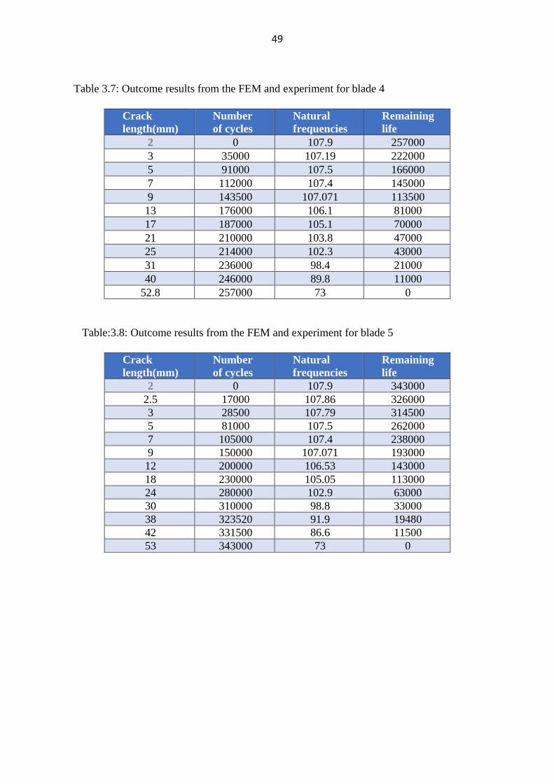
3.3.2 Tables of results generated from finite element model and experiment ......................... 46
Page 6
v
3.8 Conclusion ......................................................................................................................... 52
Chapter 4 Case study implementation of new method ............................................................ 53
4.1 Introduction ........................................................................................................................ 53
4.2 Maximum likelihood estimate ........................................................................................... 53
4.2.1 Maximum likelihood for a simple Weibull (2 parameters) ............................................ 53
4.2.2 Maximum likelihood Estimate for 3 Weibull parameters using Newton method .......... 56
4.2.3 Computation of the data using fmincon algorithm under MATLAB .......................... 61
4.2.4 Optimal decision making with the PHM ........................................................................ 62
4.2.5 Application of the optimal decision making using simulation procedure ...................... 62
Chapter 5 Interpretation of results ........................................................................................... 68
5.1 Interpretation of the results ................................................................................................ 68
5.1.1 Interpretation of the K-S test results ............................................................................... 68
5.1.2 Interpretation of the obtained PHM curve ...................................................................... 69
5.1.3 Introduction of noise in the covariate of the PHM .......................................................... 70
5.1.4 Randomising the failure level ......................................................................................... 71
Chapter 6 Conclusion and recommendations .......................................................................... 76
6.1 Conclusion ......................................................................................................................... 76
6.2 Recommendations .............................................................................................................. 77
References ................................................................................................................................ 79
Page 7
vi
Notation
ADI Average inter- demand interval
AHM Additive hazards model
ARL Applied research laboratory
AFTM Accelerated failure time models
CM Condition monitoring
CMS Condition monitoring system
CV Coefficient of variation
𝐶𝑓 Cost of unexpected failure renewal
𝐶𝑝 Cost of planned preventive renewal
DIC Digital image correlation
𝐸(𝐹𝑡) Expected value
EWMA Exponentially weighted moving average
FEM Finite element method
FGP Fault growth parameters
𝐹𝑡+1 Forecast demand per period at a given time
FCL Fatigue crack length
𝐺𝑡 Time inter demand at time t
ℎ(𝑡, 𝑍(𝑡)) Instantaneous conditional probability of failure at time t, given the
value of the covariate.
IMS Intelligent maintenance system
IPDSS Intelligent prediction decision support system
K Stress intensity factor
K-S test Kolmogorov Smirnov test
L Likelihood
ML Maximum likelihood
MDTB Mechanical diagnostic test bed
PHM Proportional hazards model
POM Proportional odds model
𝑃𝑡 Time inter demand interval
PWP Prentice William Peterson model
Page 8
vii
𝑄(𝑑) Probability that failure replacement will occur
R (𝑇𝑖) Reliability of the component function of time
𝑅(𝑇, 𝑍(𝑡)) Reliability at time 𝑇𝑖 considering the time dependent covariate
RNN Recurrent neural network
RUL Remaining useful life
SBA Syntetos Boylan approximation
SES Single exponential smoothing (SES)
TPM Transition probability matrix
𝑊(𝑑) Expected time until replacement
𝜙(𝑑) Expected average cost per unit time
𝑋𝑡 Actual demand at a given time
𝑍𝑡 Magnitude of the demand
𝜶 Smoothing constant
𝛽 Weibull shape parameter
𝛾 Weibull location parameter
𝜂 Weibull scale parameter
𝜇 Mean of historical demand
Page 9
1
Chapter 1 Introduction
1.1 Problem statement
Nowadays, the management of assets is becoming a point of central interest for the
competitiveness of organizations. One of the most important life-cycle phases in asset
management is the operation and maintenance of the asset. An efficient maintenance
program also assumes proper management of spare parts inventory.
When managing an asset, it is critical to plan and control the spare parts inventory to
avoid premature part replacement and overstocking of unnecessary spare parts (Yam, et
al., 2001). That is why forecasting the demand of spare parts is important. In fact,
forecasting is vital to every business organization and for every spare parts inventory, for
it enables estimating the spare parts stock as accurately as possible. A better forecasting
technique might allow a more efficient spare parts management policy, as well as cost
optimization.
However, several traditional forecasting methods, applied for spare parts management,
are inefficient for intermittent demand patterns and cannot accomplish reliable
forecasting results. This includes methods such as the time series method, the Croston
method and the exponential smoothing method.
Instead of using the classical methods to forecast spare parts demand, recent research
proposes an integrated method that combines condition monitoring information with
event data associated with the spare parts. The advantage related to this integrated
method is the precision estimation of parts failure, and it also avoids downtime of
machinery and stock-out. It detects potentially broken parts sufficiently early and allow a
just-in-time maintenance and spare parts availability when managing a supply system
(Hellingrath & Cordes, 2014).
The aim of this dissertation is to propose an alternative forecasting method based on
condition-based maintenance instead of using the traditional methods. The proposed
alternative method will be mixing both, event and condition monitoring data by means of
a statistical model called the proportional hazards model which is a prognostic model,
able to estimate the risk of failing for a component subject to condition monitoring.
Page 10
2
The added value brought by this alternative method is that it improves the shortcomings
and bridges the gap present in the traditional approach method, for the condition
monitoring will track the progressive advance of failure in the component.
Afterward, as soon as the prognostics result from the proportional hazards model is
available, the result will serve as input to effectively forecast the spare parts demand. The
proactive failure information received through the condition monitoring model allows
just-in-time maintenance and spare parts availability to be regulated in such a way that
the inventory management avoids premature part replacement and overstocking of
unnecessary spare parts.
1.2 Literature review
1.2.1 Spare parts forecasting overview
During the life cycles of equipment, they are used and eventually become obsolete, or fail
because of age related failure mechanisms such as fatigue, which necessitates component
replacement (Callegaro, 2010). Nowadays, with the growth of technology in industry, the
problem of spare parts management is becoming important in maintenance, not only from
a technical perspective but also from financial and economic points of view.
Companies where capital goods are made or used, typically have large inventories
(Dekker, et al., 2011). In the aerospace and automotive industries, a wide range of service
parts are held in stock, and the implication of holding spare parts in the inventory is
important for the equipment performance. Wang and Syntetos (2011), reported that in the
United States Air Force (USAF), the cost of recoverable spare parts amounted billions of
dollars in the past years, which represents 52 percent of the total cost inventory.
The interest in forecasting spare parts demand is therefore growing at an unprecedented
rate. Given that insufficient inventory stock lead to the extension of the equipment
downtime, and excessive inventory stocks lead to the immobilization of money, it is
important to determine an optimal level of spare parts to keep the equipment operating
profitably. This makes forecasting spare parts demand a crucial field for researchers.
1.2.2 Spare parts features, demand pattern and classifications
a. Spare parts features
Page 11
3
There are characteristics that distinguish spare parts from all other materials in the
industries or service system (Callegaro, 2010). The main characteristic resides in the
consumption aspect: the demands of spare parts in a company can follow very different
patterns. One of the patterns described by the demand of spare parts is intermittency (it
means the demand takes place irregularly with variable quantity). Another distinctive
characteristic of spare parts concerns the specificity of their use. They must be used only
for the use of the function for which they have been acquired. This exposes one to the
risk of obsolescence which is faced when decisions are made on replacement of capital
equipment. Very often a set of spare parts cannot be re-used on newly acquired
equipment (Callegaro, 2010).
b. Spare part demand and classification
Service spare parts are complex in modern companies. According to the type of
maintenance which is performed (i.e. preventive or corrective maintenance) it is
important to highlight that the demand which arises from preventive maintenance can be
scheduled, but remains stochastic in terms of size, whereas demand arising from
corrective maintenance is stochastic in terms of failure occurrence but deterministic in
size (Wang & Syntetos, 2011). However, both preventive and corrective maintenance
imply the intermittent nature of the demand.
Often, spare parts forecasting is complicated because the demand takes place with
irregular times, as well as the number of spare parts also vary with every instance. Such
type of demand is also intermittent, meaning that the demand occurs infrequently with
long periods of time without demand at all.
In the study of spare parts forecasting, intermittent demand patterns are very complex to
deal with because of the dual sources of variation, namely, demand arrival and demand
size (Wang & Syntetos, 2011). In the following paragraph, attention will be paid to
determine parameters which affect the spare parts demand pattern.
To evaluate and classify the two main sources of variation, namely demand arrival and
demand size causing the complexity of dealing with the intermittent demand, two
parameters are generally used:
Page 12
4
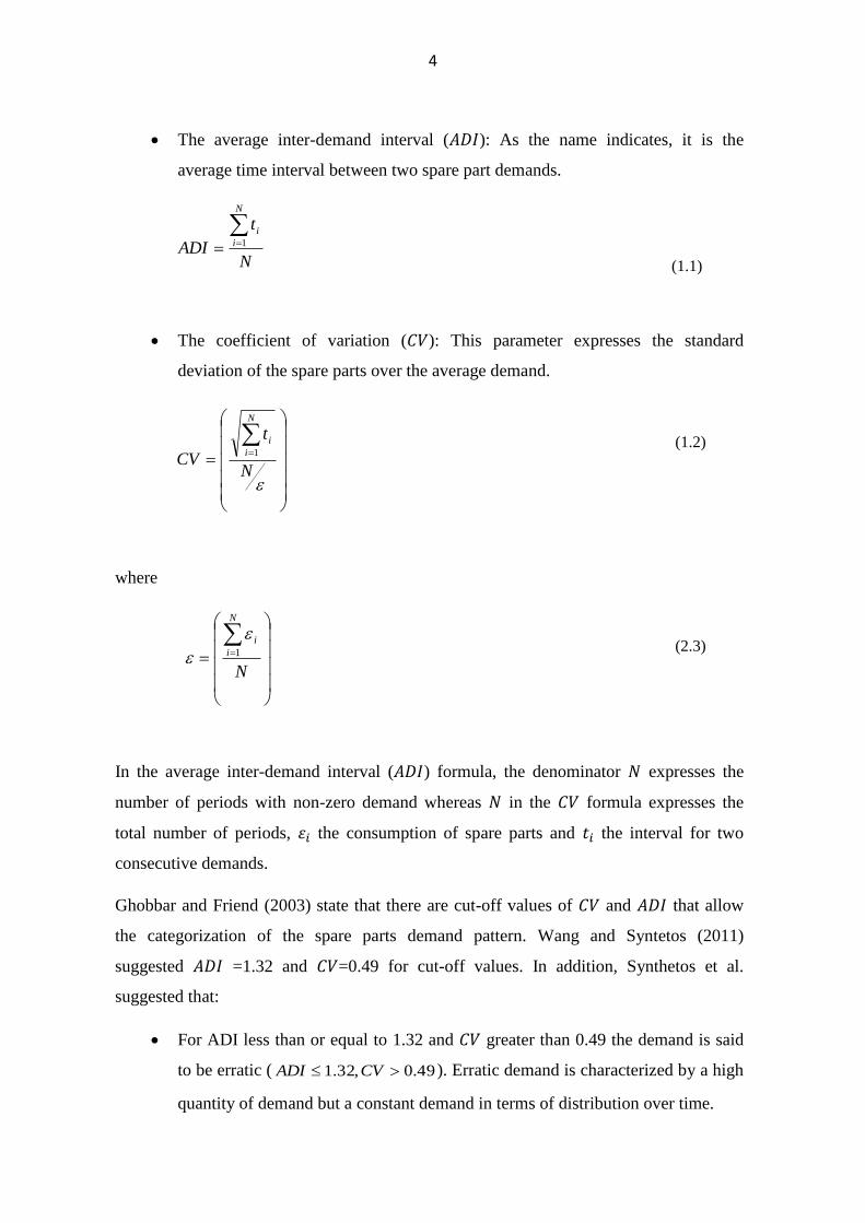
• The average inter-demand interval (𝐴𝐷𝐼): As the name indicates, it is the
average time interval between two spare part demands.
N
t
ADI
N
i
i== 1
(1.1)
• The coefficient of variation (𝐶𝑉): This parameter expresses the standard
deviation of the spare parts over the average demand.
=
=
N
t
CV
N
i
i
1
(1.2)
where
=
=
N
N
i
i
1
(2.3)
In the average inter-demand interval (𝐴𝐷𝐼) formula, the denominator 𝑁 expresses the
number of periods with non-zero demand whereas 𝑁 in the 𝐶𝑉 formula expresses the
total number of periods, 𝜀𝑖 the consumption of spare parts and 𝑡𝑖 the interval for two
consecutive demands.
Ghobbar and Friend (2003) state that there are cut-off values of 𝐶𝑉 and 𝐴𝐷𝐼 that allow
the categorization of the spare parts demand pattern. Wang and Syntetos (2011)
suggested 𝐴𝐷𝐼 =1.32 and 𝐶𝑉=0.49 for cut-off values. In addition, Synthetos et al.
suggested that:
• For ADI less than or equal to 1.32 and 𝐶𝑉 greater than 0.49 the demand is said
to be erratic ( 49.0,32.1 CVADI ). Erratic demand is characterized by a high
quantity of demand but a constant demand in terms of distribution over time.
Page 13
5
• For 𝐴𝐷𝐼 strictly greater than 1.32 and 𝐶𝑉 strictly greater than 0.49 the demand is
said lumpy ( 49.0,32.1 CVADI ), lumpy demand is one of the more complex
demand patterns to control because of many intervals with zero demand as well
as great change in the quantity.
• For 𝐴𝐷𝐼 less than or equal to 1.32 and 𝐶𝑉 less than or equal to 0.49
)49.0,32.1( CVADI the demand pattern is said to be smooth moving which
is characterized by low rotation of the system.
• For ADI, strictly greater than 1.32 and CV less than or equal to 0.49
)49.0,32.1( CVADI ) the demand pattern is said to be intermittent. The
categorization of the demand pattern will be based on the characteristics of
demand data derived from the CV and ADI parameters.
Source: From thesis: “Forecasting method for spare part demand” (Callegaro, 2010).
1.2.3 Traditional forecasting method
Forecasting can be classified into four basic types: Causal relationship, qualitative, time
series and simulation (Jacobs & Chaise, 2013).
When considering the future demand of spare parts in the production industries, decision
makers use classical statistical methods to forecast future spare parts demand. Some of
the well-known forecasting methods are exponential smoothing and regression analysis.
However, it is crucial to highlight the uncertainty in forecasting spare parts because of the
Page 14
6
long period with zero demand. The Croston method is one of the common methods to
address the intermittent demand pattern problem.
Croston (1972) found shortcomings in the single exponential smoothing methods. He
showed that a bias related to putting the most weight on the most recent demand, led to
the highest demand estimates just after the occurrence of the demand and lowest before
one (Callegaro, 2010). Croston proposed a solution to the problem by using the average
interval between demand and the average size of non-zero demand. Johnston and Boylan
(1996) worked on a revision of the Croston method by establishing that the ADI must be
greater than 1.25 for seeing the benefit of Croston over exponential smoothing.
Furthermore Syntetos & Boylan (2005) highlighted an error in the derivation done by
Croston and introduced a factor to correct the Croston formula. The modified Croston
method by Syntetos and Boylan is known as Syntetos Boylan approximation (SBA).
The focus of the following section is the time series which is a type of forecasting that is
based on data relating to past demand. Several methods belong to the time series class,
such as: simple moving average, weighted moving average, and exponential smoothing.
The following section addresses only the Croston method which is used for intermittent
demand of spare parts.
Croston Method
The single exponential smoothing method (SES) did not explicitly consider the important
parameter of the period with zero demands, whereas this is most common for spare parts
(Dekker, et al., 2011). The Croston method proposes a solution to cope with this problem
by using an alternative approach that considers both demand size and inter-arrival time
between demands. The Croston method is today well-known in industry and is
incorporated in several forecasting software packages (Teunter & Sani, 2009).
Several authors have assessed the Croston method since 1972. In 1973 Rao corrected
some expressions in the Croston paper but this did not affect the conclusion. Syntetos and
Boylan (2005) found that Croston method is biased. In 2005 they proposed an improved
version of Croston’s method, the SBA. A new Croston type method was proposed by
Teunter and Sani (2009) but did not affect considerably the conclusion of the original
one.
Page 15
7
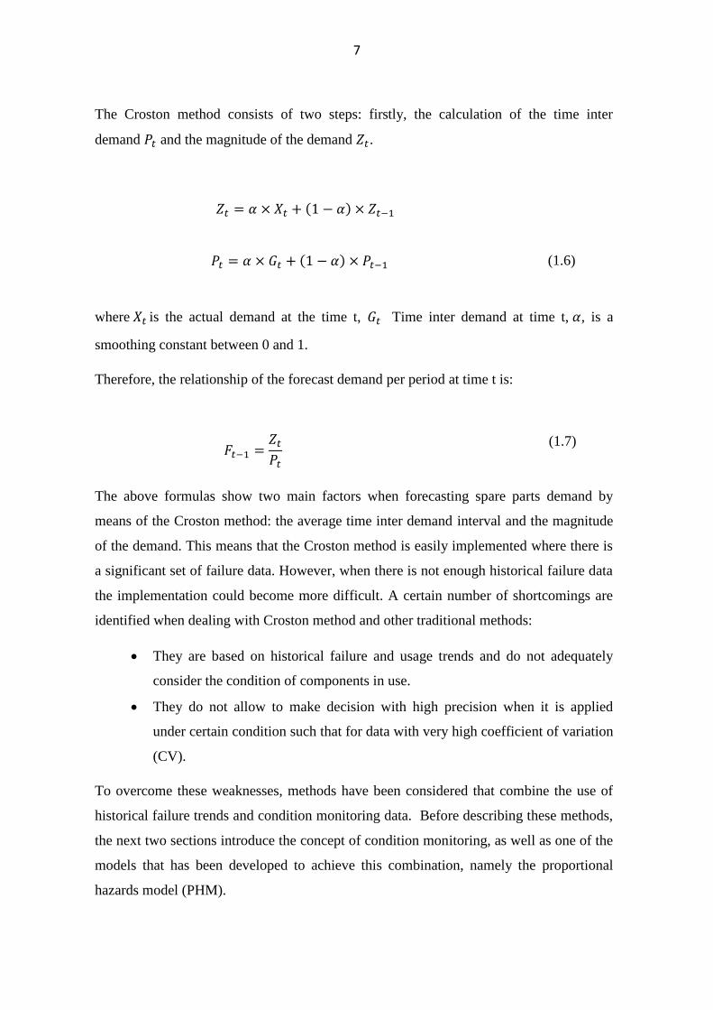
The Croston method consists of two steps: firstly, the calculation of the time inter
demand 𝑃𝑡 and the magnitude of the demand 𝑍𝑡.
𝑍𝑡 = 𝛼 × 𝑋𝑡 + (1 − 𝛼) × 𝑍𝑡−1
(1.5)
𝑃𝑡 = 𝛼 × 𝐺𝑡 + (1 − 𝛼) × 𝑃𝑡−1
(1.6)
where 𝑋𝑡 is the actual demand at the time t, 𝐺𝑡 Time inter demand at time t, 𝛼, is a
smoothing constant between 0 and 1.
Therefore, the relationship of the forecast demand per period at time t is:
𝐹𝑡−1 =𝑍𝑡
𝑃𝑡
(1.7)
The above formulas show two main factors when forecasting spare parts demand by
means of the Croston method: the average time inter demand interval and the magnitude
of the demand. This means that the Croston method is easily implemented where there is
a significant set of failure data. However, when there is not enough historical failure data
the implementation could become more difficult. A certain number of shortcomings are
identified when dealing with Croston method and other traditional methods:
• They are based on historical failure and usage trends and do not adequately
consider the condition of components in use.
• They do not allow to make decision with high precision when it is applied
under certain condition such that for data with very high coefficient of variation
(CV).
To overcome these weaknesses, methods have been considered that combine the use of
historical failure trends and condition monitoring data. Before describing these methods,
the next two sections introduce the concept of condition monitoring, as well as one of the
models that has been developed to achieve this combination, namely the proportional
hazards model (PHM).
Page 16
8
Time series methods
The focus of the following section is the time series which is a type of forecasting that is
based on data relating to past demand. Time series forecasting predict the future using
past data. A certain number of methods belong to time series, such as: simple moving
average, weighted moving average, exponential smoothing etc. The following section
addresses only methods used for intermittent demand for spare parts.
Single exponential smoothing (SES)
When forecasting the future by the mean of the SES method, the most recent occurrences are
more important than the distant past data (Jacob et al., 2014).
Concerning spare parts forecasting, SES is particularly suited for low period forecast and uses a
series of weights, where the values of the weights are decreasing in an exponential manner.
1.2.4 Condition monitoring
Condition monitoring can be described as using external parameters such as vibration,
acoustics, oil analysis, temperature, pressure, moisture, humidity, weather, or
environmental data to measure the condition of a system (Hellingrath & Cordes, 2014)
Considering the present growth of competitiveness in the industrial environment, most
organizations plan to increase their performance and productivity. However, for them to
reach the set goal and deliver the intended service required by customers, attention must
be focused on the condition of assets in the organization. To better assess the condition of
the asset or component, condition monitoring is viewed as the most effective tactic. Over
the past few decades condition monitoring became popular because of its efficient role in
detecting potential failures, and the use of condition monitoring results in the
improvement of the availability of the plant production as well as the decrease of the cost
of downtime.
Condition monitoring is a cornerstone of condition-based maintenance. When dealing
with condition-based maintenance, which is a proactive maintenance strategy, two
aspects should be considered: diagnostics and prognostics. Diagnostics uses recorded
condition information to identify, detect and isolate a fault condition whereas prognostics
consists of predicting the occurrence of the failure and estimate the remaining useful life
Page 17
9
of the asset or component to make a suitable decision concerning the optimal replacement
time of the component.
In this dissertation, a case study is presented that focuses on constructing a prognostic
model for fan axial blades, prone to fatigue failure.
1.2.5 Introduction to the proportional hazards model
(Cox, 1972) presented a model to estimate mortality risk, called the proportional hazards
model (PHM). The PHM incorporates the effects of covariates or explanatory variables
on the distribution of the lifetimes. Covariates are any measured parameters that are
thought to be related to the lifetimes of components. For each given time, the covariate
provides an increase or decrease in the hazard. proportional to the baseline hazard rate.
The model proposed by Cox (1972), was first applied for biomedical data. Some years
later the model was considered as a revolution in reliability engineering. In this context
PHM is defined as a statistical procedure for the estimation of the risk for a component to
fail when its condition is monitored (Jardine & Tsang, 2013).
The PHM is now one of the most popular statistical models used for survival analysis. Its
popularity arises from the fact that the proportional hazards model is part of a broader
class of survival analysis which provides information on the duration of time between the
identifiable start and the occurrence of an event (Leclere, 2005). A key feature when
using a proportional hazards model is that it can utilize time series variation in the
covariates. The information can be provided based on the change in explanatory variables
over time, that influence the probability of the event occurring.
The PHM is often presented in terms of the hazard model formula:
ℎ(𝑡, 𝑍(𝑡)) = ℎ0(𝑡)𝑒∑ 𝛾𝑖𝑍𝑖(𝑡)𝑝𝑖=1
(2.1)
where )(tZ i is the explanatory or predictor variable expressing the hazard at time t for
an item or a component with a given specification of a set of predictor variables denoted
by covariate. The ℎ0(𝑡) part is the baseline hazard; it includes time but not covariates, the
second part 𝑒∑ 𝛾𝑖𝑍𝑖𝑝
which is the exponential part includes covariates but not time,
therefore the Cox model equation says that the hazard at a given time is the product of
Page 18
10
two important quantities whose the baseline hazard function and the exponential
expresses the linear sum of 𝛾𝑖𝑍𝑖.
The PHM formulation assumes that:
• The renewal times (event times) are iid (independent and identically distributed.
• All the significant covariates must be part of the model.
The PHM provides the possibility of incorporating condition monitoring results into the
calculation of failure risk, where the condition parameters will be considered as
covariates. As discussed in the next section, it is considered as one of the possible
techniques that may be used to integrate the use of condition monitoring data into spare
parts forecasting.
1.2.6 Integrating condition monitoring and spare parts forecasting
To overcome the shortcomings of the traditional spares forecasting methods, (Hellingrath
& Cordes, 2014) explored the conceptualization of an approach for integrating condition
monitoring information and spare part forecasting methods. In this work it was first
shown that progress has been made in maintenance by forecasting the occurrence of
failure for a component or a technical system, estimating the remaining useful life (RUL)
using models such as the Proportional hazards models, neutral networks, etc. In addition,
it was shown that the main problem today lies on forecasting spare part demand. In fact,
several classical forecasting methods exist and are used, such as the time series,
explanatory variable and hybrid methods; but these methods present a certain number of
limitations which reduce the quality and accuracy of forecasting, to solve the problem
related to the accuracy of the spare parts demand. Hellingrath and Cordes (2014) in their
work decided to integrate condition monitoring information captured from the intelligent
maintenance system (IMS) with the “traditional” forecasting methods.
To be able to implement the integrated model, many factors should be considered
(Hellingrath & Cordes, 2014):
• The category of spare parts (for each category, different forecasting methods
are used)
• The type of output data from the IMS (it affects the modality)
• Identification of the parameters that must be adapted
Page 19
11
Regarding the above, it is important to notice that for each forecasting method, numerous
requirements and parameters can be identified, independent of the type of the IMS output
data. This implies that it is difficult to establish a guideline or general approach for the
integration needed (Hellingrath & Cordes, 2014).
Nevertheless, the spare parts demand forecasting can be addressed in different ways
(Hellingrath & Cordes, 2014):
• The first, which is the focus of this dissertation, consists of building a
proportional hazards model from the condition-based information, then
determine from there the ordering decision for spare parts when the related
component is monitored by a condition monitoring system (CMS).
• The second way, which was the aim of Hellingraph and Cordes (2014) consists
of integrating CM data with the classical forecasting model. This approach is
called CBMF and follows a sequence of steps proposed by Bacchetti &
Saccani (2011).
Pre-processing is performed to categorize of the spare parts as slow moving, intermittent,
erratic or lumpy. In addition, the main idea in this step consists of integrating CM
information and forecasting methods to generate a hybrid two step estimation
(Hellingrath & Cordes, 2014). The first step refers to the determination of the forecasting
parameters. The CM information is analysed regarding the distribution parameter of
potential breakdowns, for the second step, a Bayesian approach is used to provide a
probability function of the spare parts demand.
Wang and Aris (2011) worked on linking forecasting to equipment maintenance. Their
approach consisted of answering two main questions:
• Why is the demand for spare parts intermittent?
• How can we use models developed in maintenance research to forecast such
demand?
Furthermore, it was shown in their work that it is difficult to forecast intermittent demand
patterns because of the dual source of variation (demand arrival and demand size). In
addition, their work attempts to answer the second question by comparing demand
forecast methods and maintenance-based method (time delay forecasting methods).
Page 20
12
Forecasting spare parts demand is becoming a huge area of research in maintenance, the
main purpose in this work is to improve quality of the spare parts forecasting by making
it as accurate as possible.
Considering the weaknesses related to the usual traditional methods, Romeijnders et al.
(2012) proposed a method called two step forecast method. The advantages related to this
method is first the fact that it considers the type of component repaired, moreover
contrary to other methods, the two-step method can use information on planned
maintenance and repair operations to reduce forecast error by up to 20 % Romeijnders et
al. (2012). The first step of the method it is all about forecasting, for each type of
component the number of repairs per time unit and the number of spare part needed per
repair. Secondly these forecasts are combined to forecast demand of the spare part
Romeijnders et al. (2012).
Real data from Fokker Services (which is a company that maintains and repairs aircraft
components) captured for a period of 10 years was used to compare the two-step method
with several traditional methods.
Even though the two-step method offers better results than the Croston forecasting
method and the Syntetos Boylan approximation, which are among the best, the two- step
method still does not consider the actual condition of the component (condition
information) but it uses the historical data set.
Bacchetti and Saccani (2011) explored spare parts classification and demand forecasting
for stock control. Finally, they concluded that a gap still exists between research and
practice concerning the field addressed in this work. In their investigation, they recognize
that several aspects concur in making demand and inventory management for spare parts
a complex matter. Some of these aspects are the high number of parts managed, and the
presence of intermittent or lumpy demand patterns.
It is important to highlight that little progress has been made to date in terms of
integrating condition monitoring information into spare parts management. Bacchetti and
Saccani (2011) report that there still exists a gap between research and practice in spare
parts management. Integrating condition monitoring information captured from a
computerised maintenance management system with the traditional forecasting method,
promises possible improvement of the traditional forecasting method. The following table
Page 21
13
displays the classification of forecasting methods for sporadic demand referring to
Hellingrath and Cordes (2014).
Page 22
14
Table 1.1: Classification of forecasting methods for sporadic demand
(Hellingrath & Cordes, 2014)
Forecasting method
Classification
Consideration of the sporadic characteristic of spare parts demand
Usage of condition related information T E H O
SMA, SES × No No
EWMA × No No
Holt and Holt-Winters
× Yes No
Croston and its modifications
× Yes No
Bootstrapping × Yes No
Filtering /clustering
× Yes No
Advance demand information
× No No
Failure rate analysis
× Yes Utilizing historical data of the installed base of technical systems
Operating condition analysis
× Yes Considering influence of the environment (e.g. temperature)
Regression × Yes No
Neural networks
× No No
Bayesian approaches
× Yes Condition information is used to adjust to the demand value
Proportional hazards model
× Yes Condition information is used to adjust the demand value
Installed base forecasting
× × × × Yes Utilizing data about the condition of the installed base of technical systems
Forecasting methods in table 1.1 are classified in time series (T), explanatory (E), hybrid
(H), and other methods (O), (Bacchetti & Saccani, 2011). The proportional hazards
model is the focus in this research, for reasons outlined below.
Page 23
15
1.2.7 Selection of the proportional hazards model for this work
Several traditional forecasting methods applied to spare parts management are inaccurate
and cannot accomplish appropriate forecasting results. Methods such as Croston,
exponential smoothing, moving average and single exponential smoothing are traditional
time series method and still the most commonly used in business practice. However, the
issue with these methods is that they overestimate the mean level of intermittent demand
if applied immediately after a demand occurrence. The aim of the present study is to
develop an integrated method that combines condition monitoring information and spare
parts forecasting methods by means of PHM, as per the highlighted forecasting method
shown in Table 1.1 above. The advantages of such an integrated model would be the
precise estimation of part failure because it considers the condition of the component,
thereby avoiding downtime of machinery and stock out, by sufficiently early detection of
potential failures and allowing a just in time maintenance and spare parts availability.
1.3 Scope of the work
The demand for spare parts in industry can follow different patterns. Forecasting
intermittent demand patterns with a long period of zero demand remains particularly
challenging. One of the traditional forecasting methods which manages to address the
matter properly is the Croston method, but the shortcoming of the Croston method is that
it does not consider the condition of the component. To deal with this weakness, the
present dissertation proposes an alternative method to overcome the problem.
The approach developed in this study consists of integrating condition monitoring data
with event data by means of a proportional hazard model (PHM), to estimate the risk of
failure occurring for a component subject to condition monitoring. The statistical model
called PHM serves to forecast the spare parts demand and define spare parts management
policy.
Knowing that building a PHM requires event and condition data, both experimental and
numerical investigations were run to generate the data needed to build a PHM.
Optimal decision making is performed by means of the cost function built and based on
the PHM. It is important to highlight at this point that this dissertation does not address
aspects of the spare parts management, such as lead time, stock holding etc. It only serves
Page 24
16
to give to the inventory management the best information possible, required to make
optimal decisions.
The following approach is adopted in this dissertation:
• A numerical investigation was conducted which consisted of a modal analysis
performed with MSC.MARC2015.0 nonlinear finite element software, to
determine the coupling between natural frequency and mode shape for a 30 and
40-degree axial fan blade. A 2mm crack was initiated in the blade, then
propagated to failure. Information such as natural frequencies and mode shapes
were recorded as the crack propagated into the axial fan blade. For the purposes
of this dissertation only the natural frequency was considered as a covariate to
build the PHM.
• An experimental investigation run in the laboratory consisted of estimating the
lifetime and Paris law material constants. The setup was designed in such a way
that an initiated crack in the axial fan blade was propagated and measurements
were performed using digital image correlation (DIC). The stress intensity
factor was calculated analytically, and the measured crack length was used to
determine the Paris law constants. Furthermore, a statistical analysis was
performed on the determined material constants and lifetimes. This study was
done as a separate master’s degree study by (Brits, 2016). The experiment
served not only for validation of the finite element model (FEM) but also to
determine the Paris material constants and lifetimes which served as event data
to build the PHM.
• Both the natural frequencies generated by the FEM and the lifetimes from the
experimental investigation served as covariates and event data respectively in
the PHM.
• Instead of establishing the covariate behaviour and specifying the probability
of shifting from one state to another by means of the transition probability
matrix (TPM), a simulation procedure was performed to determine the cost
function.
• Optimal decision making is performed by means of the cost function built and
based on the PHM. An optimal risk point d was set up and served as input to
define a spare parts demand policy. It is important to highlight at this point that
Page 25
17
this dissertation does not address aspects of spare parts management which deal
with the lead time, stock holding etc. It only provides the inventory manager
information needed to make right demand of the component in a right time.
When the process described above is properly performed, it results in reduction of the
overestimation of spare parts demand, compared to the traditional forecasting methods
and a just in time spare parts management and maintenance policy is established.
Moreover, an early indication of failure provides more time for proper maintenance
planning and scheduling.
1.4 Document overview
Traditional forecasting methods as well as limitations related to these methods are
discussed in chapter 1. The advantages that these methods offer is also discussed in the
chapter. The proportional hazard model (PHM) is subsequently introduced in chapter 2 as
an appropriate statistical model to allow the integration of condition information to the
spare parts forecasting method. Chapter 2 also describes the proposed forecasting method
based on the PHM and its economics approach.
In chapter 3, an overview of a case study is presented focused on the generation of data
by means of numerical and experimental investigation. Condition monitoring data are
generated by means of the MSC.MARC/MENTAT 2016.0 software package. As the
PHM requires two types of data to be built, the event data in this work was supplied by
the experiment which is the number of loading cycles, whereas condition monitoring
data, which comprise natural frequencies, are generated by running 30-degree axial fan
blades with a 2mm initial crack inserted in the FEM.
Both event and condition monitoring data being available, in chapter 4, the
implementation of the proposed method on the case study is described. Chapter 4 also
deals with the important matter of the construction of the PHM, and the goodness of fit
testing, using the K.S test.
After constructing the PHM in chapter 4, an estimate of the risk of failure for the case
study components (fan blades) is known. Chapter 5 then discusses how to use
information from the PHM to obtain economic benefits which will lead one to define a
suitable policy for the demand or the replacement of the blades.
Page 26
18
The work is concluded in chapter 6 by showing how to use the PHM outcome for the
need of component replacement (spare parts demand). Recommendations for future work
are also made in this chapter.
Page 27
19
Chapter 2 An integrated spare parts forecasting
method using condition monitoring
2.1 Introduction
Over the past few decades, preventive maintenance decisions have been optimized by
means of statistical analysis of failure data, while condition-based maintenance has been
optimized by utilizing sophisticated methods such as vibration and oil analysis. The
present research consists of building a mixed model which combines event and condition
monitoring data into a mathematical model to predict the risk of failure occurrence for an
asset, and then use the outcome from the prediction model to forecast spare parts demand.
Reliability analysis is known as the analysis of event data only, which consists of fitting
event data to a time between probability distribution, and the fitted distribution can be
utilized for further analysis (Vlok, 1999). However, it is beneficial to combine event data
and condition monitoring data by building a mathematical model that allows maintenance
decision support (diagnostics or prognostics). In this dissertation a time dependent
proportional hazard model (PHM), which is a popular regression model is described and
utilized as a tool to forecast spare parts demand.
Renewal theory consist of estimating the reliability of a component using the recorded
time to failure and computing the renewal time that minimize the mean life cycle cost of
the future components (Vlok, 1999). When dealing with renewal theory the reliability
concepts such as failure density, cumulative failure density, reliability function and the
instantaneous failure rate are important to model the history of data in possession.
To model the reliability function of a renewable system, several approaches are used:
• A probabilistic modelling approach;
• A non-probabilistic modelling approach;
• A regression modelling approach.
The following paragraph addresses the regression modelling and particularly the
proportional hazard model.
Page 28
20
2.1.1 Regression modelling approach
Regression modelling entails merging probabilistic and non-probabilistic modelling
approaches. The following properties define the regression modelling approach:
• Like non-probabilistic models the regression models directly recognize the
existence of the survivor function or hazard rate but do not utilize the existence
of an underlying failure distribution as primary assumption.
• The regression models are not only the primary use parameter modelled but
also the concomitant information surrounding failure or covariates.
Several regressions models were identified in the literature for renewal theory:
• Accelerated failure time models (AFTM) during 1966;
• Proportional hazard model (PHM) during 1972;
• Prentice William Peterson model (PWP model) during 1981;
• Proportional Odds model (POM) during 1983;
• Additive hazard model (AHM) during 1990.
Literature shows that all the five named regression models have the same structure. The
baseline function first which is a time-based part estimated either as parametric or non-
parametric techniques, secondly an explanatory part, this part has a direct influence on
the baseline function to estimate the overall reliability of the system.
(Vlok, 1999) presented a decision matrix showing that the proportional hazard model is
the most suitable out of all the named regressions models. The criteria of evaluation were:
(1) Theoretical foundation; (2) Previous practical success in reliability modelling; (3)
Potential to lead to the dissertation objective; (4) Achievability of numerical
implementation; (5) Future potential in reliability modelling.
2.2 Proportional hazards model (PHM)
2.2.1 Development of the proportional hazards model
a. Cox proportional hazards model
The PHM is a regression model for survival time that allows for covariates, but he did not
impose a parametric form for the distribution of survival times (Crumer, 2008). Cox
(1972) assumed that the survival distribution satisfies the condition given by the formula
(2.1).
Page 29
21
b. Extension of the Cox proportional hazards model for time dependent variables
With the extended Cox proportional hazards model, covariate Z is considered as time
dependent variable. Time dependent variables are defined as variables whose values may
differ over time t , whereas time independent variables are variables which remain
constant over time.
When modelling the hazard function ℎ(𝑡), the baseline hazard function ℎ0(𝑡) can be
represented in parametric or non-parametric form. A commonly used parametric baseline
hazard function is the Weibull hazard function. To model the PHM is like the process of
regression analysis. A set of significant covariates is needed and only the significant
covariates are inserted in the models.
For a given PHM, the choice of the type of covariate to be used depend on the theoretical
assumption about the relationship between the covariate value and the hazard function
(Leclere, 2005). When the hazard function is mostly dependent on the value of the
covariates at time zero or some fixed time point, then time independent covariates are the
right choice. But when the covariates change over time and the hazard function depends
more on the current values of the covariates, then the time dependent covariates are the
right choice.
Considering errors yielded by the situation where covariates change over time, many
studies ignore the time dependence and deal with time dependent covariates as time
independent, by fixing its value at a given point in time or setting the value of the
covariate to an average value for the period that is studied. Likely problems when using
time dependent covariates as time independent or time invariant covariates are:
• As several covariates are likely to change before the advent of the event, the
variation is eliminated, and important information is lost.
• Several phenomena are generated by dynamic, longitudinal processes, because
the value of a covariate along the time path affects the probable event
happening.
• The model does not include the value of the covariate observed at the time of
event occurrence, although it may be this actual value that generate the event.
A few notes are relevant:
Page 30
22
• With the availability of software today, there are some which directly deal with
time dependent variables and the need for considering time dependent variables
as time independent is reduced.
• For the purposes of this research, event and covariate data are generated by
laboratory experiments because of the difficult access to industry data. This is
dealt with in Chapter 3.
For this dissertation, the covariates are considered time dependent and the PHM will be
addressed as follows:
• First determine the Weibull parameters (𝛽, 𝜂, 𝛾) constituting the baseline
function. This computation is done by applying the maximum likelihood
estimation method.
• Secondly the changes in the measurements of the covariate characteristics in
the explanatory part will not be modelled according to the semi–Markov
process, but through a simulation procedure.
• The third step deals with the economics - it is all about specifying the optimal
inspection time that minimizes the cost.
In the parametric PHM one of the most important operations to be done is to estimate the
𝛾′𝑠 to access the effect of explanatory variable, the corresponding estimate parameters are
determined by means of the maximization of the likelihood function Kleinbaum (1999).
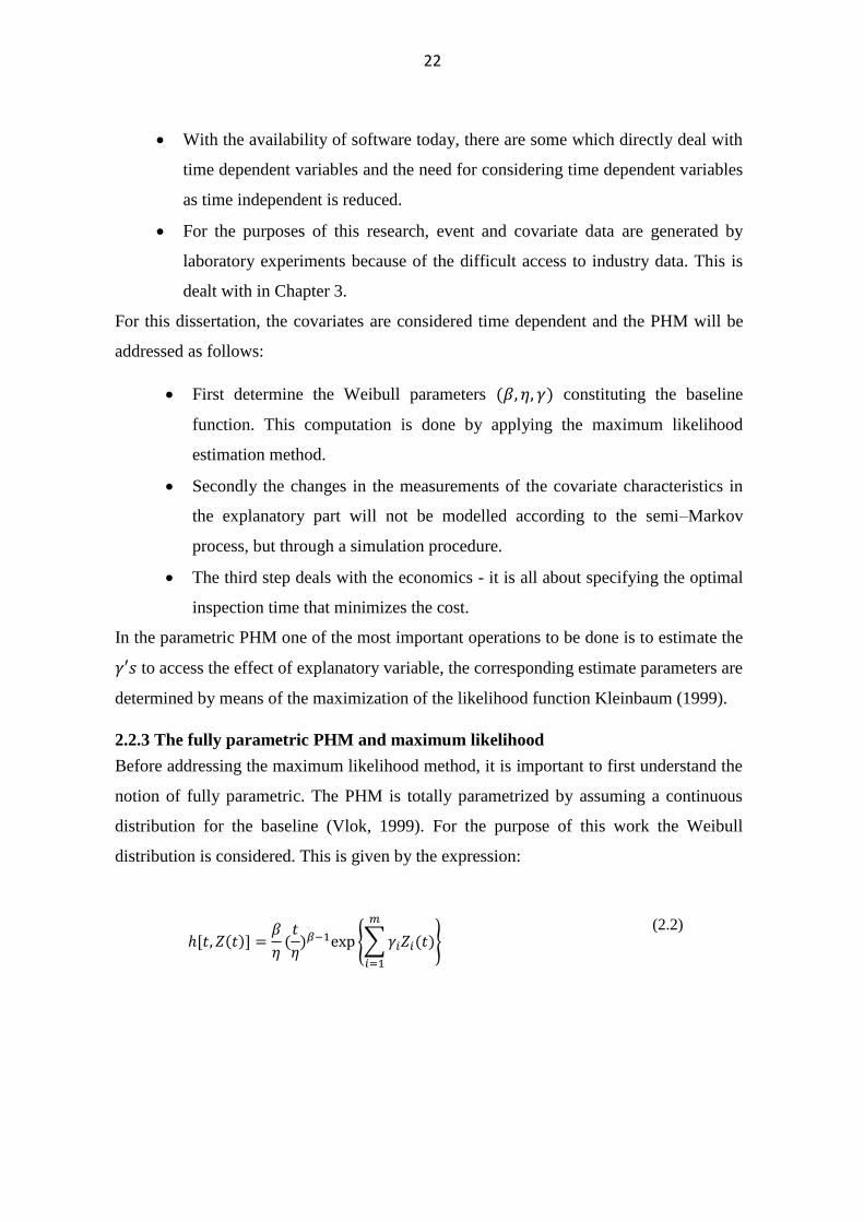
2.2.3 The fully parametric PHM and maximum likelihood
Before addressing the maximum likelihood method, it is important to first understand the
notion of fully parametric. The PHM is totally parametrized by assuming a continuous
distribution for the baseline (Vlok, 1999). For the purpose of this work the Weibull
distribution is considered. This is given by the expression:
ℎ[𝑡, 𝑍(𝑡)] =𝛽
𝜂(
𝑡
𝜂)𝛽−1exp {∑ 𝛾𝑖𝑍𝑖(𝑡)
𝑚
𝑖=1
}
(2.2)
Page 31
23
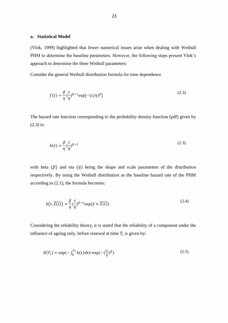
a. Statistical Model
(Vlok, 1999) highlighted that fewer numerical issues arise when dealing with Weibull
PHM to determine the baseline parameters. However, the following steps present Vlok’s
approach to determine the three Weibull parameters:
Consider the general Weibull distribution formula for time dependence
𝑓(𝑡) =𝛽
𝜂(
𝑡
𝜂)𝛽−1exp [−(𝑡/𝜂)𝛽]
(2.3)
The hazard rate function corresponding to the probability density function (pdf) given by
(2.3) is:
ℎ(𝑡) =𝛽
𝜂(
𝑡
𝜂)𝛽−1
(2.3)
with beta (𝛽) and eta (𝜂) being the shape and scale parameters of the distribution
respectively. By using the Weibull distribution as the baseline hazard rate of the PHM
according to (2.1), the formula becomes:
ℎ(𝑡, 𝑍(𝑡) ) =𝛽
𝜂(
𝑡
𝜂)𝛽−1exp (�� × 𝑍(𝑡) )
(2.4)
Considering the reliability theory, it is stated that the reliability of a component under the
influence of ageing only, before renewal at time 𝑇𝑖 is given by:
𝑅(𝑇𝑖) = exp (− ∫ ℎ(𝑡)𝑑𝑡𝑇𝑖
0)=exp (−(
𝑇𝑖
𝜂)𝛽)
(2.5)
Page 32
24
If 𝑈𝑖 = (𝑇𝑖
𝜂)𝛽, 𝑈𝑖 has a unit negative exponential distribution. As for (2.5), at time 𝑇𝑖 the
reliability of the component under the influence of time independent covariates according
to the PHM is estimated by:
𝑅(𝑡, ��)=𝑒𝑥𝑝 [− ∫𝛽
𝜂
𝑇𝑖
0(
𝑡
𝜂)𝛽−1dt exp (�� × 𝑍) ]
(2.6)
By solving (2.6) it gives:
𝑅(𝑡, ��)=𝑒𝑥𝑝 [−(𝑇𝑖
𝜂)𝛽exp (�� × ��]
(2.7)
Equation (2.6) is about the time independent covariate. For the time dependent 𝑈𝑖 =
(𝑇
𝜂)𝛽exp (𝛾, 𝑍��), again with unit exponential distribution. When dealing with this case with
time dependent covariates, the reliability at time 𝑇𝑖 for the component, considering the
time dependent covariate will be:
𝑅(𝑡, 𝑍(𝑡) =𝑒𝑥𝑝 [− ∫𝛽
𝜂
𝑇𝑖
0(
𝑡
𝜂)𝛽−1exp (�� × 𝑍(𝑡) 𝑑𝑡]
(2.8)
Equation (2.8) gives:
𝑅(𝑡, 𝑍(𝑡) =𝑒𝑥𝑝 [− ∫ exp (��𝑇𝑖
0× ��𝑖 (𝑡)𝑑(
𝑡
𝜂)𝛽]
(2.8)
Considering 𝑈𝑖= ∫ exp (��𝑇𝑖
0× ��𝑖 (𝑡)𝑑(
𝑡
𝜂)𝛽, with unit negative exponential distribution. In
practice (2.8) and (2.9) are approximated by:
𝑅(𝑡, 𝑍(𝑡) =𝑒𝑥𝑝 {∑ exp (𝛾 𝑖𝑘=1 × 𝑍𝑖
∗ (𝑡𝑘)) × [(𝑡𝑘+1
𝜂)𝛽 − (
𝑡𝑘
𝜂)𝛽]}
(2.9)
with 0=𝑡0 < 𝑡𝑖 < ⋯ < 𝑇𝑖 inspection points where covariate measurement was performed
and 𝑍𝑖∗ = 0.5 × (𝑍𝑖 (𝑡𝑘
) + 𝑍𝑖 (𝑡𝑘+1)).
Page 33
25
a. Maximum likelihood (Parameter estimation)
As indicated in the literature, the maximum likelihood of the Cox model parameters is
found by maximizing a likelihood function. The likelihood function is a mathematical
expression which describes the joint probability of obtaining the data observed on the
subjects in the study as a function of the unknown parameters (the 𝛾′𝑠) in the model
being considered (Kleinbaum, 2000). Some literature such as, (Vlok, 1999), addressed
the optimization of the likelihood equation to determine the Weibull parameters.
The Weibull parameters are estimated by maximizing the likelihood equation given by:
𝐿(𝛽, 𝜂, ��)=∏ ℎ(𝑇𝑖, 𝑍𝑖 (𝑇𝑖
𝑖 ) × ∏ 𝑅(𝑇𝑗, 𝑍𝑗(𝑡)) 𝑗
(2.10)
with the 𝑖 index referring to failure times and where 𝑗 = 1,2 … … … . . 𝑛 indicate failure
and suspension times. It is important to highlight that for the aim of this dissertation it
deals with complete data.
The Weibull parameters 𝛽, 𝜂, 𝛾 which maximize (2.19), can also maximize
log (𝐿(𝛽, 𝜂, 𝛾) or 𝑙(𝛽, 𝜂, 𝛾). It is numerically appropriate to maximize 𝑙(𝛽, 𝜂, 𝛾) which is
given by:
𝑙(𝛽, 𝜂, 𝛾 ) = 𝑟𝑙𝑛 (𝛽
𝜂⁄ ) + ∑ 𝑙𝑛 [(𝑇𝑖
𝜂⁄ )𝛽−1] + ∑ ��
𝑖𝑖
× 𝑍𝑖 ( 𝑇𝑖) − ∑ ∫ exp (��
𝑇𝑗
0𝑗
× 𝑍 ��(𝑡) 𝑑(𝑡
𝜂⁄ )𝛽
(2.11)
where r is the number of failure renewals.
In this dissertation, equation (2.11) or (2.12) are solved numerically using a Newton-
Raphson optimization procedure.
𝑙(𝛽, 𝜂, 𝛾 ) = 𝑟(−𝛽𝑙𝑛𝜂) + 𝑟𝑙𝑛𝛽 + (𝛽 − 1) × ∑ 𝑙𝑛𝑡𝑖 + ∑ 𝛾𝑏𝐵𝑏 − [exp(𝑎) × (∑ 𝛾𝑔𝑍𝑗𝑔𝑖 ) × (𝑡𝑖(𝑗+1)
𝛽− 𝑡𝑖𝑗
𝛽
𝑛
𝑖=1
)]𝑚
𝑏=1
𝑟
𝑖=1
(2.12)
Page 34
26
To maximize equation (2.12) and estimate the three Weibull parameters, a number of
techniques have been tested successfully. Among these are:
• A Nelder-Mead method
• A BFGS Quasi-Newton method
• Snyman’s dynamic trajectory method
• A modified Newton-Raphson method
The performance of the above-mentioned methods was assessed regarding their economy,
which means according to the number of iterations needed to converge, the number of
objective function evaluations and the number of partial derivative evaluations, as well as
robustness. The outcome from the evaluation of the above-mentioned methods was such
that the Newton Raphson method was found more suitable and economic for optimization
of the maximum likelihood function. This dissertation uses the Newton Raphson method
to optimize the equation (2.12).
b.1 Newton Raphson method for a 3 parameters Weibull
Vlok (1999) proposed a template to simplify the computation of the Newton Raphson
optimization technique for vibration monitoring data. Referring to the suggested
template, 𝑛 expresses the number of histories, which is seven for this dissertation, and i
indicates the history number such that: 𝑖 = 1,2 … . . 𝑛.
The time to failure or suspension in each history, as expressed by 𝑇𝑖, and 𝐶𝑖, are used as
indications making the difference between failure and suspension. For 𝐶𝑖=1, 𝑇𝑖 is a failure
and for 𝐶𝑖 = 0, 𝑇𝑖 is a suspension. For the aim of this dissertation, data are complete,
means without suspensions.
The number of inspections 𝑘𝑖 must be set to be able to model the scenario associated to
the time dependent covariate which is the natural frequency. For the aim of this
dissertation a 50000 cycle is set as interval between inspection to build the proposed
templates.
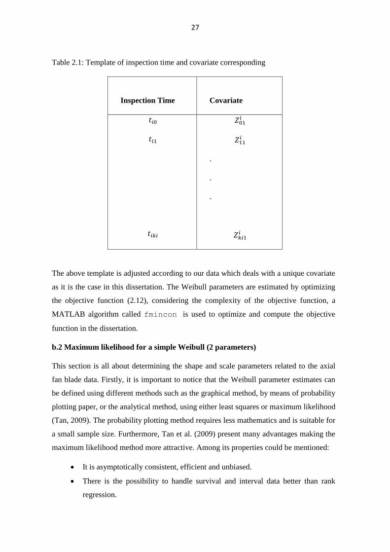
Below in table 2.1 at the sample of the template associated to our data is given.
Page 35
27
Table 2.1: Template of inspection time and covariate corresponding
Inspection Time
Covariate
𝑡𝑖0
𝑡𝑖1
.
.
.
𝑡𝑖𝑘𝑖
𝑍01𝑖
𝑍11𝑖
.
.
.
𝑍𝑘𝑖1𝑖
The above template is adjusted according to our data which deals with a unique covariate
as it is the case in this dissertation. The Weibull parameters are estimated by optimizing
the objective function (2.12), considering the complexity of the objective function, a
MATLAB algorithm called fmincon is used to optimize and compute the objective
function in the dissertation.
b.2 Maximum likelihood for a simple Weibull (2 parameters)
This section is all about determining the shape and scale parameters related to the axial
fan blade data. Firstly, it is important to notice that the Weibull parameter estimates can
be defined using different methods such as the graphical method, by means of probability
plotting paper, or the analytical method, using either least squares or maximum likelihood
(Tan, 2009). The probability plotting method requires less mathematics and is suitable for
a small sample size. Furthermore, Tan et al. (2009) present many advantages making the
maximum likelihood method more attractive. Among its properties could be mentioned:
• It is asymptotically consistent, efficient and unbiased.
• There is the possibility to handle survival and interval data better than rank
regression.
Page 36
28
Considering that the lifetime T of the axial fan blades follows a Weibull distribution with
𝛽 and 𝜂 parameters, the probability density function could be given by:
𝑓(𝑡) =𝛽
𝜂(
𝑡
𝜂)𝛽−1𝑒
−(𝑡𝜂
)𝛽
(2.13)
with t , the failure time, beta the shape parameter strictly greater than zero and eta the
scale parameter. Considering 7=N failures as shown in the data, the log likelihood
function is given by:
Λ = 𝑁𝑙𝑛(𝛽) − 𝑁𝛽 ln(𝜂) + (𝛽 − 1) ∑ ln(𝑡𝑖) − ∑(𝑡𝑖
𝜂)𝛽
𝑁
𝑖=1
𝑁
𝑖=1
(2.14)
Referring to the Newton Raphson method, the above (2.14) log likelihood function
maximization, gives:
1
𝛽=
∑ 𝑡𝑖𝛽
𝑙𝑛𝑡𝑖𝑁𝑖=1
∑ 𝑡𝑖𝛽𝑁
𝑖=1
−1
𝑁∑ 𝑙𝑛𝑡𝑖
𝑁
𝑖=1
(2.15)
As the log likelihood function maximization is dealt with numerically, a MATLAB
optimization code is used to solve (2.15).
The estimated parameters obtained from the likelihood function maximization are utilized
to build the PHM. The PHM obtained is tested to know how well it fits the data, therefore
the goodness of fit is applied to assess the constructed model.
2.2.4 Economical approach with the PHM
The PHM provides us with the approximate risk of failing for the component based on
the age and covariates (the natural frequency for the case study in this dissertation). The
information which is made available by the PHM should be utilized to obtain economic
benefits
Page 37
29
a. How to use PHM outcome for economic benefit?
Vlok (1999) states: “Economical benefits from a statistical failure analysis can be
guaranteed with a high confidence level if the minimum long-term life cycle cost LCC of
a component is determined and pursued’’.
Long term life cycle cost (LCC) concept
The LCC in renewal analysis arise from two important quantities in practice:
• The cost of unexpected renewal (failure cost 𝐶𝑓)
• The cost of preventive replacement (𝐶𝑝)
Equilibrium must be obtained between the risk of having to spend 𝐶𝑓 and the advantages
in the cost difference between 𝐶𝑓 and 𝐶𝑝 without wasting useful life of a component. The
optimum economic preventive renewal time will be at this balance point.
b. LCC for Weibull PHM
For optimal decision making with the PHM in reliability, Makis and Jardine (2013) made
a model available. The model specifies the optimal renewal policy in terms of an optimal
hazard leading to the minimum LCC. To be able to determine the hazard rate which leads
to the minimum LCC it is needed to predict the behaviour of covariates.
Makis and Jardine’s model assumes the covariate behaviour to be stochastic and
approximating it by a non - homogeneous Markov chain in a finite space. Referring to
that model, the expected average cost per unit time is a function of the threshold risk level
given by:
∅(𝑑) =𝐶𝑝 + 𝐾𝑄(𝑑)
𝑊(𝑑)
(2.16)
where, 𝑄(𝑑) = 𝑃(𝑇𝑑 ≥ 𝑇) represents the probability that failure replacement will occur
and 𝑊(𝑑) the expected time until replacement and 𝐾 = 𝐶𝑓 − 𝐶𝑝.
Jardine et al. (1997) state that the calculation of the functions defined by the probability
that failure replacement will occur Q(d) and the expected time until replacement W(d),
Page 38
30
can sometimes take a long time, due to the covariates quantity and structure, sometimes a
simulation procedure could be used to determine the cost function, in this project such a
simulation procedure is used to determine the cost function and the optimal risk point
which minimizes the risk.
2.2.5 Goodness of fit for the PHM
The assumptions characterizing PHM are well defined for the time independent
covariates: (1) Renewal times are iid (identically distributed); (2) The influential
covariates are inserted in the model building; (3) the ratio of two hazard rates for given
covariates should be constant over time.
Several approaches can be used to evaluate the goodness of fit for the PHM, more often
residual analysis using graphical methods as well as statistical tests are used to assess at
which point the PHM fits the data.
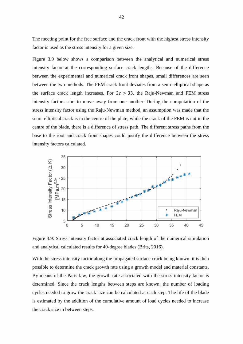
The advantage of the analytical method is that it provides statistical tests with a
corresponding p-value to assess the PHM assumptions for covariates. It also gives the
ability to make a correct and clear decision (Kleinbaum, 2000).
a. Graphical methods
To test the assumptions of the PHM, several graphical methods can be used. These
include:
• Cumulative hazard plots
• Average hazard plots
• Residual plots
Out of the three mentioned categories of graphical methods mentioned, residual plots are
the more common. To construct these residual plots, the Cox- generalized residuals for
PHM are used.
Several methods are performed to calculate the residual in Cox regression model, among
them are (1) Schoenfeld; (2) score residuals; (3) Martingale and (4) deviance. Each of
these has a specific utilization, such as goodness of fit, which serves to identify possible
outliers and the influential observations (Jin, 2014).
In survival analysis the diagnostics procedure for the model checking is focused on
residuals. In this dissertation graphical techniques will not be used to assess the goodness
Page 39
31
of fit for the PHM even though in many publications residual plots are often used under
different ways such as: (1) the residual against order of appearance; (2) ordered residuals
against expectation etc.
a. Analytical methods
The use of graphical tests is often mixed with the analytical or statistical test as it is the
case with the EXAKT software which uses the graphical residual analysis and the K-S
test. However, because of the diversity of interpretation from analysts, the analytical
approach seems more advantageous for decision making. Several statistical tests can be
used, below are discussed some:
b.1 Wald test
The Wald test allows one to assess the quality of the parameters obtained from the
maximum likelihood. Therefore, for the PHM, this method can test the values of 𝛽, 𝜂 and
𝛾 that are obtained. The Wald test statistic for a given coefficient is given by:
𝑊𝑖 =𝑛(𝜃𝑖)2
𝑣𝑎𝑟(𝜃𝑖)
(2.17)
𝑣𝑎𝑟(𝜃𝑖) being the variance of the regression coefficient for a sample size expressed by n.
The calculation of the p-value is made from the 𝜒2 distribution.
b.2 K-S test (Kolmogorov Smirnov)
The K-S test is a statistical hypothesis test. It is a non-parametric method used to
generally compare the actual data to a normal distribution; the cumulative probability
function of the data is compared with the cumulative probability function of a theoretical
normal distribution.
However, in the context of the PHM this test is applied on the residual of the PHM. As it
is known that the residual of the proportional hazard model must have an exponential
distribution, the K-S test is then used to compare the cumulative distribution function of
the PHM, residuals and the cumulative distribution function of an exponential
distribution.
Page 40
32
The null hypothesis: The cumulative distribution function of the PHM residuals is equal
to the cumulative distribution function of an exponential distribution fitted on the
residuals.
The null hypothesis testing is made by checking whether the critical value 𝐷𝛼, which is
found in the K-S table according to the level of significance, set is less or greater than 𝐷
which is the calculated (𝐷-statistic).
The 𝐷 − statistics is defined as the largest absolute difference between the PHM
residuals cumulative distribution function and the cumulative exponential distribution.
The 𝑝 − value is the probability of obtaining a sample more extreme than the ones
observed.
Acceptance criteria: If 𝐷 < 𝐷𝛼 for a given significance level, the null hypothesis should
be accepted;
Rejection criteria: If 𝐷 > 𝐷𝛼 the null hypothesis should be rejected.
2.3 Flowchart illustration of the integrated method
The following diagram expresses the use of PHM to forecast spare parts demands:
PHM BUILDING
ECONOMIC APPROACH
Step 1: It consists of building the PHM with the outcome from the maximum likelihood
function, in this dissertation a MATLAB algorithm allowed the computation of the
Newton Raphson objective function.
GOODNESS OF FIT TEST
SELECT THE SUITABLE ‘d’
DECISION MAKING
JIT SPARE DEMAND
Page 41
33
Step 2: The goodness of fit testing is performed to assess how well the PHM fits the data,
the Kolmogorov Smirnov is the statistical test used in this dissertation.
Step 3: The blending of the PHM and economic consideration is performed at this level.
The outcome from this step is the optimal risk point that minimizes the cost during the
simulation procedure d.
Step 4: The selected d point allows gives the critical number of loading cycle
corresponding to each component.
Step5: The information obtained from the previous step is used to make decisions about
the right time to make the component replacement.
Step 6: The replacement is performed according to the critical point pre-defined, which
means there is no need of stocking too much spares because the right time for
replacement is known, means JIT (just-in-time) spare parts demand.
The integrated forecasting method being proposed in this chapter, before the
implementation of the given method in a case study in chapter 4, the following chapter
introduces the case study and describes the generation of data needed to implement the
new method on the case study.
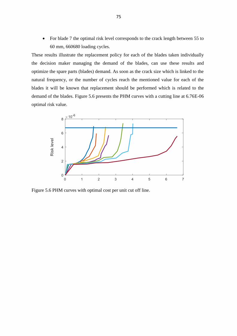
Page 42
34
Chapter 3 Case study description
3.1 Introduction
This chapter addresses the numerical and experimental investigation carried out to make
available event and condition monitoring (CM) data needed to build the PHM. The case
study focuses on a turbomachinery 30-degree fan axial blade.
The reason for considering the turbomachine blade failure case in this study, was simply
to capitalise on the numerical models and experimental results that were already available
from a prior study conducted by Brits (2016). In his work Brits worked on estimating the
fatigue crack life (FCL) of turbomachine blades by means of a fatigue tests in the
laboratory. As part of this study Brits conducted extensive numerical investigations and a
very comprehensive experimental study. Because of the dearth of results of this nature in
the open literature, these results were used for the current investigation. The author of this
dissertation also assisted Brits in executing the experiments described here, to make sure
that he has a full understanding of the intricacies of the data.
However, unlike the work by Brits where the main goal was to estimate the fatigue crack
life of turbomachinery blades, here the same blades were considered with a focus on
updating the finite element model to get the natural frequencies corresponding to the
FCL. Then both the FCL and natural frequencies obtained were used as inputs to build a
PHM prognostic model. The choice of natural frequency as covariate is since it is easy to
measure, compared to the actual crack size which is difficult to directly measure in
practice. The numerical investigation which was conducted by the current author, using
the models generated by Brits, allowed calculation of the natural frequencies related to
the crack propagation.
It is important to note that blade lifetime was not obtained from the finite element model
(FEM). Only the stress intensity factors were used as input to the Paris Law model and a
modal analysis was run by means of MSC.MARC/MENTAT 2016.
The experimental investigation by Brits was carried out in the C-AIM Labs at the
University of Pretoria and entailed the use of a 50 kN spectral dynamics electrodynamics
shaker to apply base excitation to the axial fan blade specimens. The fatigue lifetime
recorded from the experimental approach served as event data required to build the PHM.
Page 43
35
After having obtained the outcomes from both numerical and experimental investigations,
the PHM could be constructed from both types of data made available through numerical
and experimental investigations.
Tables and curves associated with both the numerical and experimental approaches are
provided in this dissertation. The CM and event data generated are computed as a
’likelihood’. The outcome from the likelihood function are Weibull estimate parameters
needed to build the PHM.
3.2 Numerical investigation
(Brits, 2016) followed a FEM approach to identify the natural frequencies corresponding
to the crack growth. Furthermore, from the FEM, he calculated the stress intensity factor
(SIF) that correlate to specific surface crack lengths. The calculated SIF and material
constant obtained after the experiment served as input to a Paris law growth model to
specify the crack growth rate. The number of loading cycles were correlated to the crack
propagation. Figure 3.1 shows the mains steps characterizing the numerical investigation:
• FEM set up
• Crack insertion
• SIF calculation
• Growth rate
• Life prediction
Figure3.1: Numerical investigation approach (Brits, 2016)
This dissertation utilized the FEM designed by Brits (2016), the FEM was performed to
estimate the fatigue crack life of an axial fan blade. However, for the aim of this
dissertation the mentioned FEM was extended to obtain the natural frequency
Page 44
36
corresponding to the propagation of the crack, then the obtained natural frequencies
served as covariate to the PHM.
3.2.1 FEM set up
Two types of the axial fan blade specimen are considered in this dissertation: the 30 and
40-degree but only the 30-degree is used for building the PHM at the end of the work.
Considering the computational cost, a static structural analysis was run with a set periodic
tip displacement of ±10mm. The base of the blade was clamped in all directions at the
attachment point, whereas a single point displacement is utilized at the extreme tip of the
blade. The location of that point is selected similarly as the laser displacement transducer
was in the experiments.
Table 3.1 shows the material properties, and figure 3.2 the model of a 40-degree blade,
including the boundary condition.
Figure 3.2: Finite Element Model of a 40-degree blade with boundary conditions (Brits,
2016)
The table below gives the material properties for the finite element model
Table3.1: Material properties chosen for FE model
Structural Property Values Elasticity Modulus E 69 GPa
Tensile Strength 220 MPa Yield Stress 165 MPa
Density 2830 kg/m3 Poisson Ratio 0.33
Page 45
37
The following flowchart shows systematic process to build the finite element model for
an axial fan blade using MSC.MARC/MENTAT2015.0 with an initiated and propagated
crack.
Figure 3.3: Flowchart of model set up in MSC.MARC/ MENTAT 2016 (Brits, 2016).
The validation of the boundary conditions and material properties were done by means of
mesh convergence and modal analysis. To establish the maximum size of 4-nodded
tetrahedral elements for having an accurate result within a reasonable computational time,
a mesh convergence study was performed.
The result of the finite element and experimental modal analysis was that the first three
modes and their natural frequencies are similar. The FEM natural frequency result shows
a maximum error of 7.92% on the second mode compared to the experimental modal
analysis result, which is the mean between the test specimens.
Table 3.2 results indicate that the modelling parameters selected approach those of the
real blades, thus, it is used further in the study.
Page 46
38
Table 3.2: Natural Frequency results for 40-degree blades
Experiment (Hz) FEM (Hz)
Error (%)
Mode 1 105,3 104,92 3,19 Mode 2 428,5 462,44 7,92 Mode 3 667,5 674,82 1,1
For final validation, the experimental and numerical strains at 10mm tip displacement are
compared. Figure 3.4 to Figure 3.7 below respectively show the strain field before the
initiation of the crack for the experimental and numerical approaches.
When there is no load applied, the noise floor of the readings is measured, since it is an
offset in the strain readings. Considering figure 3.4 the determination of the strain noise
gives +0.0793 percent and –0.0042 percent. The maximum strain of 0.274 percent was
measured on the base of the blade as shown at figure 3.5.
The major strain field was obtained from the numerical approach, where the base of the
blade gives a maximum strain of 0.2078 percent. Regarding the noise floor, the
experimental and numerical strain fields for the test specimen differ by 6.73 percent for
the maximum major strain. The results in our possession shows that the finite element
model set up is right and can accurately represent the axial fan blades.
Figure 3.4: Experimental maximum principal strain fields of a 40-degree blade at (a) Zero
load and at (b) 10mm tip displacement.
Page 47
39
Figure 3.5: Experimental maximum principal strain fields of a 30-degree blade at (a) Zero
load and at (b) -10mm tip displacement.
Figure3.6: Numerically computed major strain field of a 40-degree blade at -10mm tip
displacement (Brits, 2016).
Page 48
40
Figure 3.7: Numerically computed major strain field of a 30-degree blade at -10mm tip
displacement (Brits, 2016).
3.2.2 Crack insertion
The MSC.MARC/ MENTAT software gives the user the ability to freely add cracks into
the model, the size and shape of the crack to be added are arbitrary. Regarding the model
under analysis in this dissertation, a crack with a surface length of 2 mm was seeded. The
crack propagation was used to obtain the natural frequencies and was not used to obtain
lifetime information.
After each load cycle at an increment of 1 mm, the crack propagates from the initial seed.
The crack growth is done by the means of a scaling function which scales the crack by
taking the relationship of the stress intensity factor (MSC software, 2016, pp.158-162).
Page 49
41
Where d is the scaled crack growth size, and 𝑑0 is the user defined crack growth size per
increment.
The software automatically does the remeshing, while the crack is propagating. The
remeshing works along with the global meshing and focuses on the mesh at and around
the crack front.
The cracked finite element axial fan blade showing an extended crack with its meshes
shown below.
Figure 3.8: Cracked FE model axial fan blade showing extended crack with mesh. (Brits,
2016) To reduce errors when remeshing, the direction of the crack growth was chosen
only as mode 1. Same results were obtained when the maximum hoop stress theory was
used to determine the crack growth.
3.2.3 Summary of the results from Brits (2016) dissertation
With the propagation of the crack in the blade, the stress intensity factors are computed at
distinct points in the crack front for each crack size by the means of 3D VCCT.
𝑑 = 𝑑0(∆𝐾𝐼
∆𝐾𝑀𝐴𝑋)𝑚
(3.1)
Page 50
42
The meeting point for the free surface and the crack front with the highest stress intensity
factor is used as the stress intensity for a given size.
Figure 3.9 below shows a comparison between the analytical and numerical stress
intensity factor at the corresponding surface crack lengths. Because of the difference
between the experimental and numerical crack front shapes, small differences are seen
between the two methods. The FEM crack front deviates from a semi–elliptical shape as
the surface crack length increases. For 2𝑐 > 33, the Raju-Newman and FEM stress
intensity factors start to move away from one another. During the computation of the
stress intensity factor using the Raju-Newman method, an assumption was made that the
semi–elliptical crack is in the centre of the plate, while the crack of the FEM is not in the
centre of the blade, there is a difference of stress path. The different stress paths from the
base to the root and crack front shapes could justify the difference between the stress
intensity factors calculated.
Figure 3.9: Stress Intensity factor at associated crack length of the numerical simulation
and analytical calculated results for 40-degree blades (Brits, 2016).
With the stress intensity factor along the propagated surface crack being known. it is then
possible to determine the crack growth rate using a growth model and material constants.
By means of the Paris law, the growth rate associated with the stress intensity factor is
determined. Since the crack lengths between steps are known, the number of loading
cycles needed to grow the crack size can be calculated at each step. The life of the blade
is estimated by the addition of the cumulative amount of load cycles needed to increase
the crack size in between steps.
Page 51
43
The surface crack length at the number of load cycles predicted using the mean values of
𝑚 and 𝐵 from the 40- degree test specimens as shown in figure 3.11.
Finally, the predicted FCL (fatigue crack length) correlates well with the mean of the
experimental FCL result. Thus, the determined Paris law material constants are valid and
the approach to predict FCL shows real promise.
Figure 3.10: Predicted fatigue crack length vs number of load cycles compared to
experimental results for a 30-degree blade (Brits, 2016).
Figure 3.11: Predicted fatigue crack length vs number of load cycles compared to
experimental Results for a 40-degree blade (Brits, 2016).
Page 52
44
3.2.4 Method validation
For the reason of validation, the 30-degree blade geometry was used with the same model
parameters as the 40-degree blade, with the only difference in the validation model the
geometry. Boundary conditions, material properties as well as the mesh configuration
being the same for the 30 and 40-degree model. This would allow us to determine the
model sensitivity for changes in geometry.
Furthermore, this would also provide insight in why the 30-degree test specimen had a
longer FCL than the 40-degree test specimens.
a. Natural frequencies
A modal analysis was performed to ensure that the material properties and modelling
constraints have been chosen correctly so that the model represents the real blade.
Table 3.3 shows the numerical and the average experimental natural frequencies. A
maximum error of 5.8 percent exists between the two, and it can be concluded that the
parameters chosen are close enough.
Table 3.3: Natural frequency result for the 30-degree blades
Experiment
(Hz) FEM (Hz)
Error
(percent)
Mode 1 107.2 107.86 4.79
Mode 2 506.3 483.7 4.46
Mode 3 768.8 724.2 5.8
a. Strain
Considering the 30-degree blade, the major strain fields from the FEM and the
experiments as shown in Fig 3.4 and 3.5 respectively, the noise floor during the test is +
0.0833 percent and -0.0006 percent. The maximum strain at -10 mm tip displacement is
0.2292 percent at the base of the blade. The maximum computed strain is 0.158 percent,
also present at the base of the blade, which means that the numerical strain values differ
by 8.5 percent from that of the experiment.
The errors values being small, it can be concluded that the physics-based model of the
30-degree blade does indeed approximate a real 30-degree axial fan blade.
Page 53
45
The major strain in the 30-degree test specimens is lower than the 40-degree test
specimens, it implies a lower stress and a longer fatigue crack life. In the figure 3.8 is
shown the bending stress results for the 30-degree blade, as well as the maximum stress is
123.1MPa, 31.4MPa less than the stress experienced by the 40-degree blade.
c. Life prediction
Similarly, for the 40-degree blade, the stress intensity factor calculates as function of
surface crack length and the FCL estimation was done for the 30-degree blade. Figure
3.10 and 3.11 shows the predicted crack growth using FEM and the mean material
constant values is obtained in the experimental investigation.
3.3 Experimental investigation
Lifetime and Paris law material constants are obtained by means of the experimental
investigation. In this section an experimental setup is designed and utilized for the
initiation and propagation of the crack. Figure 3.12 shows an overview of steps undertook
to obtain lifetime:
• Experimental set up
• Crack growth measurement
• Stress intensity calculation
• Material constant determination
• Statistical analysis
3.3.1 Experimental set up
Figure 3.12: Experimental investigation overview (Brits, 2016)
During the experiment, to apply the base excitation to the test specimens, a 50 kN
Spectral dynamics electrodynamics shaker was used. The advantage of the chosen shaker
is that it has a larger displacement at high frequencies compare to other available
Page 54
46
equipment in the laboratory. The acquisition of data during the experiment was
performed by means of a 4M DIC system from Gesellschaft fur Optische Messtechnik
(GOM) by taking images of the test specimens before and during loading. Figure 3.13
shows the experimental setup.
Figure 3.13: Experimental setup showing (a) Right side view, (b) Left side view, (c) The
mounted test specimen. (Brits, 2016)
3.3.2 Tables of results generated from finite element model and experiment
In this section the data generated from the experiment performed by Brits (2016) and the
natural frequency results were generated by the reviewed finite element model. It is
important to highlight that the finite element analysis was extended to allow for the
Page 55
47
calculation of the natural frequencies for the first mode from the initiated crack to the
failure for 30-degree and 40-degree axial fan blade, because this was not included in Brits
(2016) study.
Table of experimental and numerical data
Figure 3.12 presents an overview of the steps taken to determine the constants used in the
Paris Law to obtain the lifetime. Figure 3.8 shows that the design of the experimental set
up was such that a crack initiates and propagates in an axial fan blade. The use of DIC
(digital image correlation) allowed the measurement of the crack during a post processing
procedure. The measured crack growth and the analytically determined stress intensity
factors were then used to determine the material constants for the Paris Law. Several
experiments with the same loading parameters were conducted, after which a statistical
analysis on lifetime and Paris Law material constant was possible. Tables below represent
the results from section 3.2.3 and the extended FEM that was performed in this
dissertation to generate natural frequency related to the crack propagation.
Table 3.4: Outcome results from the FEM and experiment for blade 1
Crack
length(mm)
Number
of cycles
Natural
frequencies
Remaining
life
2 0 107.9 169700
2.5 21400 107.86 148300
4 43200 107.59 125800
6 59400 107.53 110300
9 75700 107.071 94000
11 91200 106.7 78500
18 108200 105.05 61500
24 121900 102.9 47800
27 128200 100.6 41500
31 141900 98.4 27800
38 148900 91.9 20800
45 162890 81.7 6810
53 169700 73.1 0
Page 56
48
Table 3.5: Outcome results from the FEM and experiment for blade 2
Crack
length(mm)
Number
of cycles
Natural
frequencies
Remaining
life
2 0 107.9 185000
2.6 16000 107.85 169000
3.5 39000 107.6 146000
5 67000 107.56 118000
6 75000 107.53 110000
10 91000 106.9 94000
13 97000 106.1 88000
15 112000 105.6 73000
19 127000 104.5 58000
25 142000 102.3 43000
31 157000 98.4 28000
39 179000 91.4 6000
52.9 185000 73.1 0
Table 3.6: Outcome results from the FEM and experiment for blade 3
Crack
length(mm)
Number
of cycles
Natural
frequencies
Remaining
life
2 0 107.9 240000
2.3 12000 107.86 228000
3 35000 107.79 205000
4 45000 107.59 195000
7 80000 107.4 160000
9 95000 107.071 145000
12 113000 106.53 127000
15 128000 105.6 112000
19 167000 104.5 73000
25 198000 102.3 42000
30 205000 98.8 35000
40 230000 89.8 10000
53.1 240000 73.1 0
Page 57
49
Table 3.7: Outcome results from the FEM and experiment for blade 4
Crack
length(mm)
Number
of cycles
Natural
frequencies
Remaining
life
2 0 107.9 257000
3 35000 107.19 222000
5 91000 107.5 166000
7 112000 107.4 145000
9 143500 107.071 113500
13 176000 106.1 81000
17 187000 105.1 70000
21 210000 103.8 47000
25 214000 102.3 43000
31 236000 98.4 21000
40 246000 89.8 11000
52.8 257000 73 0
Table:3.8: Outcome results from the FEM and experiment for blade 5
Crack
length(mm)
Number
of cycles
Natural
frequencies
Remaining
life
2 0 107.9 343000
2.5 17000 107.86 326000
3 28500 107.79 314500
5 81000 107.5 262000
7 105000 107.4 238000
9 150000 107.071 193000
12 200000 106.53 143000
18 230000 105.05 113000
24 280000 102.9 63000
30 310000 98.8 33000
38 323520 91.9 19480
42 331500 86.6 11500
53 343000 73 0
Page 58
50
Table 3.9: Outcome results from the FEM and experiment for blade 6
Crack
length(mm)
Number
of cycles
Natural
frequencies
Remaining
life
2 0 107.9 402000
3 12500 107.79 389500
5 89000 107.5 313000
7 134000 107.4 268000
10 209000 106.9 193000
13 239000 106.1 163000
20 303000 104.1 99000
26 339000 101.6 63000
32 374000 97.9 28000
40 389000 89.8 13000
46 397000 79.5 5000
49 399500 75.1 2500
53.05 402000 73 0
Table 3.10: Outcome results from the FEM and experiment for blade 7
Crack
length(mm)
Number
of cycles
Natural
frequencies
Remaining
life
2 0 107.9 665000
3 50000 107.79 615000
5 130000 107.56 535000
7 180000 107.4 485000
9 254000 107.071 411000
13 330000 106.1 335000
17 430000 105.1 235000
21 500000 103.9 165000
25 550000 102.3 115000
33 600000 97.4 65000
38 630000 91.9 35000
44 654000 82.7 11000
52.95 665000 73 0
Tables 3.11 and 3.12 document the natural frequencies as functions of crack lengths that
were not included in the analyses performed by Brits (2016). He did not focus on
presenting the natural frequencies trend as the crack was propagating. However, this
project needs two types of data, namely event data (lifetime of the blades) and condition
monitoring data (natural frequencies).
Page 59
51
Table 3.11: Natural frequencies and corresponding crack length for 30- degree fan axial
blade
Increment
Crack Length
(mm)
Natural
Frequencies (Hz)
1 0.0020 107.900
2 0.0037 107.649
3 0.0057 107.595
4 0.0075 107.449
5 0.0093 107.071
6 0.0109 106.938
7 0.0126 106.532
8 0.0141 106.101
9 0.016 105.601
10 0.0177 105.050
11 0.0195 104.525
12 0.0212 103.917
13 0.0229 103.181
14 0.0245 102.389
15 0.0261 101.592
16 0.0278 100.644
17 0.029 99.723
18 0.0304 98.874
19 0.032 97.910
20 0.0347 95.576
21 0.0357 94.228
22 0.0372 92.949
23 0.0386 91.438
24 0.0401 89.892
25 0.0406 87.934
26 0.0423 86.027
27 0.0436 83.935
28 0,0454 81.685
29 0.0469 79.117
30 0.0473 76.446
31 0.0530 73.000
Page 60
52
Table3.12: Natural frequencies and corresponding crack length for 40-degree fan axial
blade
Increment Crack Length (mm)
Natural Frequency
(Hz)
1 4.194 104.923
2 7.963 103.36
3 11.413 101.774
4 15.197 100.142
5 18.757 97.157
6 21.979 94.560
7 25.075 91.973
8 27.876 89.476
9 30.603 87.06
10 33.437 84.329
11 35.839 80.601
12 38.879 76.832
13 42 73.180
3.8 Conclusion
Having the event data from the experiment and the condition monitoring data available
from the FEM, all inputs required to build the PHM are now available. The following
chapter therefore deals with the implementation of the PHM for the case study presented
in chapter 3.
The choice of natural frequency as covariate is justified by the fact that it is relatively
easy to measure (i.e can be measured at different points on the structure without affecting
the results). Natural frequency is a global parameter of a structure, as opposed to a local
parameter such as mode shape. It is further uniquely related to the stiffness of the
structure if one may assume that mass is essentially constant - which is for practical
purposes the case except in erosive or very dirty environments. Natural frequency can
therefore be indicative of change of stiffness, which may again be assumed to indicate
damage.
Page 61
53
Chapter 4 Case study implementation of the
proposed method
4.1 Introduction
This chapter covers the implementation of the integrated forecasting method by following
steps described in section 2.3.2 expressing the use of the PHM to forecast the spare parts
demand. The chapter commences by estimating the parameters required to build the
proportional hazard model (PHM), after conducting statistical tests to evaluate how well
the PHM fits the data. Parameter estimates are determined by maximizing the likelihood
function by means of the Newton Raphson method. Risks are then blended with the
economics to optimize the decision making with the proportional hazards model, by
setting a threshold point which is referred to as the ‘d’ point. This point may finally be
used by decision makers in inventory to forecast spare parts demand and do a just in time
spare parts management.
The failure of the 30-degree blade as was described in chapter 3 is used as the case study
to demonstrate the proposed method to forecast spare parts demand.
4.2 Maximum likelihood estimate
As described in section 2.2.3 b, maximum likelihood estimation is a well-known method
to allow estimation of the regression coefficients needed to build a PHM. Having event
and condition data available from the numerical and experimental investigation, the
Weibull parameters of equation (2.2) may be estimated by maximization of equation
(2.10).
4.2.1 Maximum likelihood for a simple Weibull (2 parameters)
In section 2.2.3, the maximum likelihood of the log function (2.14) gives the following
equation:
1
𝛽=
∑ 𝑡𝑖𝛽
𝑙𝑛𝑡𝑖𝑁𝑖=1
∑ 𝑡𝑖𝛽𝑁
𝑖=1
−1
𝑁∑ 𝑙𝑛𝑡𝑖
𝑁
𝑖=1
To determine the shape parameter 𝛽 in the above equation requires the log likelihood
function maximization. As the equation is dealt numerically, a MATLAB code was
Page 62
54
written related to the above formula to determine the shape parameter, the output from
the MATLAB code gave a shape parameter 𝛽 = 2.17.
The differentiation of the equation (4.5) with respect to 𝜂 gives:
𝜂 = (1
𝑁∑ 𝑡𝑖
𝛽𝑁𝑖=1 )
1𝛽⁄
=1
7∑ 𝑡𝑖
2.177𝑖=1 = 366700.8 cycles
The following steps are required to determine the simple (2 parameters) Weibull model:
Step 1: With 𝛽 = 2.17 and 𝜂 = 366700.8 cycles the hazard function for the fan axial
blades are given by:
ℎ(𝑡) =2.17
366700.8(
𝑡
366700.8)1.17
Step 2: Economical approach for 2 Weibull parameters (Application on the axial fan
blade data).
In this section, a time-based approach is presented that can be used to optimize the axial
fan blade replacement decision making and the economic implications.
Referring to Jardine et al. (2013), the optimal preventive replacement age of an item
subject to breakdown is given by:
𝐶(𝑡𝑝) =𝐶𝑝 × 𝑅(𝑡𝑝) + 𝐶𝑓 × (1 − 𝑅(𝑡𝑝))
𝑡𝑝 × 𝑅(𝑡𝑝) + 𝑀(𝑡𝑝)(1 − 𝑅(𝑡𝑝))
(4.1)
Considering 3/1 cost ratio which describes such that the failure cost 𝐶𝑓 in South African
Rands (ZAR) is three times the preventive cost 𝐶𝑝 with 𝐶𝑝 = 20000 𝑍𝐴𝑅 and 𝐶𝑓 =
60000 𝑍𝐴𝑅, below is given a sample of results table for blade 7.
Page 63
55
Table 4.1: Table of result for blade 7 (time-based approach)
Time (cycles)
Reliability R(t)
Cumulative distribution
F(t)
Cost per unit Time
C(tp)
1 0 1 0 Inf
2 50000 0,9868 0,0132 0,4151
3 130000 0,9 0,1 0,2026
4 180000 0,8078 0,1922 0,1815
5 254000 0,6372 0,3628 0,1902
6 330000 0,4514 0,5486 0,2185
7 430000 0,2435 0,7565 0,3574
8 500000 0,1409 0,8591 0,5819
9 550000 0,0898 0,9102 0,8319
10 600000 0,0544 0,9456 1,3957
11 630000 0,3993 0,9607 1,9113
12 654000 0,0299 0,9701 2,6871
13 665000 0,0263 0,9737 2,7521
The cost curve corresponding to the above blade is given by:
Cost
Figure 4.1: Curve of cost versus Time for blade 7
For 2 Weibull parameters or the time-based approach the optimal time which minimizes
the cost is 0.1889 ZAR per unit.
The table below 4.2 is the summary of all blade results, showing the optimal replacement
time, which minimizes the cost.
Time
e 0.1889
Page 64
56
Table 4.2: Table of results for all blades (time-based approach)
Optimal Time Reliability
Minimal Cost per Unit time
Blade1 169700 0.8 0.18
Blade 2 185000 0.79 0.18
Blade 3 167000 0.83 0.1886
Blade 4 187000 0.79 0.188
Blade 5 200000 0.76 0.188
Blade 6 239000 0.67 0.1889
Blade 7 180000 0.81 0.1815
Average 189571 0.78 0.185
Considering the time-based result presented in table 4.4, it is important to highlight that
the simple Weibull calculation, which is a time-based approach, shows that the optimal
replacement time for the blades which minimizes the cost varies between 169700 to
239000 cycles, with an average of 189571 cycles. The surprise in the above table is that
most of the blades are still reliable at the indicated replacement time. The following
section will consider the use of a proportional hazard model.
4.2.2 Maximum likelihood Estimate for 3 Weibull parameters using Newton method
Section 2.2.3 illustrate a template proposed by (Vlok, 1999) adjusting the inspection time
to the corresponding covariate. These templates are arranged in such way that they can be
easily computed in the objective function given by formula (2.12). Below is given the
summary of data for all histories in the proposed template.
Page 65
57
History 1: Table of inspection time with corresponding natural frequency
(with natural frequency as covariate)
𝑡𝑖 𝑍𝑘1 ∑ 𝑡𝑖 ∑ 𝑍𝑘
1
𝑡𝑖(𝑗𝑚)
− 𝑡𝑖𝑗
0 107.9 50000
50000 107.56 50000
100000 105.875 50000
150000 86.8 150000 300.235 50000
History 1: Table of inspection time with corresponding crack size
(with crack size as covariate)
𝑡𝑖 𝑍𝑘1 ∑ 𝑡𝑖 ∑ 𝑍𝑘
1
𝑡𝑖(𝑗𝑚)
− 𝑡𝑖𝑗
0 2 50000
50000 5 50000
100000 14.5 50000
150000 41.5 150000 61 50000
Page 66
58
History 2: Table of inspection time with corresponding natural frequency
(with natural frequency as covariate)
𝑡𝑖 𝑍𝑘2 ∑ 𝑡𝑖 ∑ 𝑍𝑘
2
𝑡𝑖(𝑗𝑚)
− 𝑡𝑖𝑗
0 107.9 50000
50.000 107.58 50000
100.000 105 50000
150.000 100.35 150.000 312.93 50000
History 3: Table of inspection time with corresponding natural frequency
(with natural frequency as covariate)
𝑡𝑖 𝑍𝑘3 ∑ 𝑡𝑖 ∑ 𝑍𝑘
3
𝑡𝑖(𝑗𝑚)
− 𝑡𝑖𝑗
0 107.9 50000
50.000 107.5 50000
100.000 106.8 50000
150.000 105.05 50000
200000 100 200000 419..35 50000
Page 67
59
History 4: Table of inspection time with corresponding natural frequency
(with natural frequency as covariate)
𝑡𝑖 𝑍𝑘3 ∑ 𝑡𝑖 ∑ 𝑍𝑘
3
𝑡𝑖(𝑗𝑚)
− 𝑡𝑖𝑗
0 107.9 50000
50.000 107.6 50000
100.000 107.45 50000
150.000 106.5 50000
200000 104.45 200000 426 50000
History 5: Table of inspection time with corresponding natural frequency
(with natural frequency as covariate)
𝑡𝑖 𝑍𝑘3 ∑ 𝑡𝑖 ∑ 𝑍𝑘
3
𝑡𝑖(𝑗𝑚)
− 𝑡𝑖𝑗
0 107.9 50000
50.000 107.70 50000
100.000 107.4 50000
150.000 107.071 50000
200000 106.53 50000
250000 103.975 50000
300000 100 300000 632.976 50000
Page 68
60
History 6: Table of inspection time with corresponding natural frequency
(with natural frequency as covariate)
𝑡𝑖 𝑍𝑘3 ∑ 𝑡𝑖 ∑ 𝑍𝑘
3
𝑡𝑖(𝑗𝑚)
− 𝑡𝑖𝑗
0 107.9 50000
50.000 107.3 50000
100.000 107.2 50000
150.000 107 50000
200000 106.5 50000
250000 105.9 50000
300000 104 50000
350000 101 50000
400000 73 400000 811.9 50000
History 7: Table of inspection time with corresponding natural frequency
(with natural frequency as covariate)
𝑡𝑖 𝑍𝑘3 ∑ 𝑡𝑖 ∑ 𝑍𝑘
3
𝑡𝑖(𝑗𝑚)
− 𝑡𝑖𝑗
0 107.9 50000
50.000 107.59 50000
100.000 107.56 50000
Page 69
61
150.000 107.52 50000
200000 107.1 50000
250000 107.071 50000
300000 106.1 50000
350000 106 50000
400000 106 50000
450000 104.5 50000
500000 103.9 50000
550000 102.3 50000
600000 97.4 50000
650000 73 650000 1110.5 50000
The computation of all histories in the objective function (2.12) is performed by means of
MATLAB package using the fmincon algorithm.
4.2.3 Computation of the data using fmincon algorithm under MATLAB
To determine the Weibull parameters 𝛽, 𝜂, 𝛾 needed to construct the PHM, the likelihood
equation (2.11) is solved numerically using Newton Raphson method which gives the
equation (2.12) which is the objective function that has been solved with the algorithm
fmincon.
fmincon algorithm is a nonlinear programming solver which allows finding the
minimum of constrained nonlinear multivariable function.
For the aim of this dissertation, the objective function given by the equation (2.12) was
minimized using the syntax: 𝑥 = 𝑓𝑚𝑖𝑛𝑐𝑜𝑛(𝑓𝑢𝑛, 𝑥0, 𝐴, 𝑏, 𝐴𝑒𝑞, 𝑏𝑒𝑞, 𝑙𝑏, 𝑢𝑏). The results
from the simulation gives: (1) 𝛽 = 1.0012 ; (2) 𝜂 = 7.10𝑒 + 05; (3) 𝛾 = 0.0293.
The PHM construction obtained from the maximum likelihood output is:
Page 70
62
ℎ(𝑡, 𝑧(𝑡)) =1.0012
7.1004𝑒 + 05(
𝑡
7.1004𝑒 + 05)(1.0012−1)exp [0.0293 × 𝑧(𝑡)]
In this dissertation, only the K-S test is performed on the residual of the data for a 30-
degree blade in the software R to evaluate how well the PHM fit the data, the output
results obtained from R was:
𝐷 = 0.49659 , 𝑝 − value = 0.06873
The above result shows that at 5 percent level of significance the null hypothesis is
accepted for 𝐷 is less than 𝐷𝛼 which is 0.565, and the 𝑝 − value being greater than 0.05,
the null hypothesis is accepted which means that the PHM fit well the data.
4.2.4 Optimal decision making with the PHM
It was specified in section 2.2.4 that after receiving the outcome from PHM which
presents the risk that the component will fail based on the integration of age and
covariate, this outcome from the PHM could only serves when using it for an economical
benefit, this introduces the notion of blending the PHM with economics addressed by
Jardine and Makis (2013). However, in this dissertation does not address the TPM
approach but a simulation approach as shown in section 4.2.5.
4.2.5 Application of the optimal decision making using simulation procedure
a. Tables of the resulting proportional hazard values for the seven experimental
blades
Table 4.3: Risk versus loading cycles for blade 1
N(cycles) PHM (Risk)
1 0 0
2 21400 1.51E-06
3 43200 1.58E-06
4 56400 1.68E-06
5 75700 1.83E-06
6 91200 1.94E-06
7 108200 2.38E-06
8 121900 2,84E-06
9 128200 3.10E-06
10 141900 3.49E-06
Page 71
63
Table 4.4: Risk versus loading cycle for blade 2
N(cycles) PHM(Risk)
1 0 0
2 16000 1.52E-06
3 39000 1.56E-06
4 67000 1.63E-06
5 75000 1.68E-06
6 91000 1.89E-06
7 97000 2.06E-06
8 112000 2.18E-06
9 127000 2.46E-06
10 142000 2.93E-06
11 157000 3.49E-06
12 179000 4.41E-06
13 185000 6.63E-06
Table 4.5: Risk versus loading cycle for blade 3
N(cycles) PHM (Risk)
1 0 0
2 12000 1.50E-06
3 35000 1.53E-06
4 45000 1.58E-06
5 80000 1.73E-06
6 95000 1.83E-06
7 113000 2.00E-06
8 128000 2.18E-06
9 167000 2.46E-06
10 198000 2.93E-06
11 205000 3.39E-06
12 230000 4.55E-06
13 240000 6.67E-06
11 148900 4.29E-06
12 162890 5.26E-06
13 169700 6.65E-06
Page 72
64
Table 4.6: Risk versus loading cycle for blade 4
N(cycles) PHM (Risk)
1 0 0
2 35000 1.53E-06
3 91000 1.63E-06
4 112000 1.73E-06
5 143500 1.83E-06
6 176000 2.06E-06
7 187000 2.32E-06
8 210000 2.61E-06
9 214000 2.93E-06
10 236000 3.49E-06
11 246000 4.55E-06
12 257000 6.62E-06
Table 4.7: Risk versus loading cycle for blade 5
N(cycles) PHM(Risk)
1 0 0
2 17000 1.51E-06
3 28500 1.53E-06
4 81000 1.63E-06
5 105000 1.73E-06
6 150000 1.83E-06
7 200000 2.00E-06
8 230000 2.39E-06
9 280000 2.85E-06
10 310000 3.39E-06
11 323520 4.29E-06
12 331500 4.82E-06
13 3433000 6.66E-06
Page 73
65
Table 4.8: Risk versus loading cycle for blade 6
N(cycles) PHM(Risk)
1 0 0
2 12500 1.53E-06
3 89000 1.63E-06
4 134000 1.73E-06
5 209000 1.89E-06
6 239000 2.06E-06
7 303000 2.53E-06
8 339000 3.02E-06
9 374000 3.60E-06
10 389000 4.55E-06
11 397000 5.42E-06
12 399500 5.92E-06
13 402000 6.67E-06
Table 4.9: Risk versus loading cycle for blade 7
N(cycles) PHM (Risk)
1 0 0
2 50000 1.54E-06
3 130000 1.63E-06
4 180000 1.73E-06
5 254000 1.83E-06
6 330000 2.06E-06
7 430000 2.32E-06
8 500000 2.61E-06
9 550000 2.93E-06
10 600000 3.31E-06
11 630000 4.29E-06
12 654000 5.12E-06
13 665000 6.65E-06
By fitting time and the corresponding covariate to the constructed PHM we get tables 4.3
to 4.9, these tables represent the risk of failing for all the blades and the corresponding
time expressed in term of number of loading cycle.
Page 74
66
b. Plotting of the resulting proportional hazard values for the seven experimental
blades
The risk ℎ(𝑡, 𝑧(𝑡)) is an instantaneous conditional probability of failure for the blade at
time 𝑡, given the value 𝑍(𝑡). Figure 4.2 indicates the plotting of risk versus the number of
loading cycles for the obtained PHM represented in section 4.2.3. Tables 4.3 to 4.9 show
the fitting of the PHM to the corresponding data which are time and covariate for all
blades:
Figure 4.2 Risk versus loading cycles for all the blades.
After determining the PHM and plotting it as shown in Figure 4.2 for all the 30- degree
axial fan blades, the following step is to establish optimal replacement decisions,
including economic considerations, based to the PHM values, where these values would
be a function of both age of the components, as well as the condition parameter. This
basically entails finding an optimum PHM risk value at which components would be
replaced. It is normally expected that such optimisation would be achieved by balancing
the risk of expensive failures (when the replacement PHM value is chosen at a too high a
level and some components may fail before reaching this value) and wasting remaining
useful life of components (when the replacement PHM value is chosen at a low level).
The trends of the PHM shown in Figure 4.2, however, show that, in this case, the
optimisation problem seems to be trivial and that the optimal replacement PHM level
would be at almost the constant PHM failure value (with some small safety factor) and
Page 75
67
that this result seems to be independent of age. With such PHM trend, the application of
PHM for spare part demand becomes useless because time does not have influence and
the forecast could be performed straight with covariate trending. In Figure 4.2 all the
blades have the risk of failing at almost the same PHM level. Table 3.4 to Table 3.10
confirm the PHM trend because the outcome from the experiment and FEM is showing
that all the blades failed at almost equal crack length 52 to 53mm and the natural
frequency at that failure point was around 72 to 73 Hz, independent of age. This is
discussed further in the next chapter.
Page 76
68
Chapter 5 Interpretation of results
The event and condition monitoring data generated in Chapter 3 for the axial flow fan by
means of the experiment and numerical simulations were processed in Chapter 4. The
Weibull parameters were obtained by minimizing the objective function given by
equation (2.12). The optimal Weibull parameters are: (1) the shape parameter 𝛽 =
1.0012 , (2) the scale parameter 𝜂 = 7.1004𝑒 + 05 and the location parameter 𝛾 =
0.0293. The mentioned Weibull parameters results served as input to construct the PHM
shown in Chapter 4, section 4.2.3.
ℎ(𝑡, 𝑧(𝑡)) =1.0012
7.1004𝑒 + 05(
𝑡
7.1004𝑒 + 05)(1.0012−1)exp (0.0293
× 𝑧(𝑡))
(5.1)
The model presented in equation (5.1) was tested to see how well it represents the data.
For this the K-S test served to verify how well the PHM fits the data. At 5% significance
level with 𝐷∞ = 0.565, the calculated 𝐷-statistic was equal to 0.49659 with a
corresponding 𝑝 −value of 0.06873. The following paragraph proposes results
interpretation starting by the K-S test.
5.1 Interpretation of the results
5.1.1 Interpretation of the K-S test results
The test statistic 𝐷 applied is simply the maximum absolute difference between two
cumulative distributions, and the p-value the area under the cumulative distribution. For
the PHM in this dissertation the null hypothesis is that the cumulative distribution
function of the PHM residuals is equal to the cumulative distribution function of an
exponential distribution. The inferences on the goodness of fit for the model (5.1) is made
on the 𝐷-statistic an 𝑝 −value. The following is the meaning of the results:
The calculated 𝐷-statistic obtained is 0.49659 and at 5% significance level the 𝐷∞ =
0.565, the corresponding p-value obtained is 0.06873. The calculated 𝐷-statistic being
less than 0.565 implies that the null hypothesis should not be rejected, moreover the p-
value obtained also goes in the same direction than the 𝐷-statistic test. By not rejecting
the null hypothesis, it means that the cdf of the PHM residuals is equal to the cumulative
Page 77
69
distribution function of the exponential distribution; therefore, the PHM constructed fits
the data well.
5.1.2 Interpretation of the obtained PHM curve
Figure 4.2 expresses the resulting PHM curves for the seven experimental blades, the
implication of the characteristics of the PHM displayed in that figure is that time has no
influence, only the covariate has influence in the obtained model. This means that the
decisions can be made based only on the covariate. In this case it would be sufficient to
advice that spare parts must be ordered when the covariate reaches a critical value. The
following curve in figure 5.1 demonstrate that the baseline of the obtained PHM is a
constant.
Figure 5.1 Hazard curve, without considering the covariate (Only baseline of the PHM).
Figure 5.1 indicates how the baseline of the PHM behaves, and since the baseline of the
Weibull PHM is essentially time based, it can be concluded that time does not have
influence on the PHM, only the covariate has an influence. Therefore, the economical
optimisation will be trivial, for the decision can be made only based by the observation of
the covariate. It is important to highlight that this situation where age does not have an
influence, would lead to the most economical replacement strategy, since replacement
decisions are then based on a highly predictive covariate measurement, with little risk of
failure or wasted life.
This result does demonstrate the universality of the PHM method for a wide range of
situations where, on the one extreme, the predictive capability of the covariate is very
Page 78
70
high (implying that the mathematics reduces the influence of age in the parameter
solution, by solving to 𝛽= 1), towards the other extreme, where the predictive capability
of the covariate is very low (and the parameter solution would yield 𝛽 >1 and 𝛾 very
small, to reduce the influence of the covariate on the age-based hazard rate).
In practice, it may be expected that to have a condition measurement which would be so
accurate in predicting the failure (which in the present case was done in laboratory
conditions), would not be common. To be able to demonstrate the application of the
PHM method (where both condition monitoring results and age plays a role) for decision-
making with economical consideration, it was decided to introduce noise or randomness
progressively in the PHM so that the risk for the seven blades is different. Two methods
were considered, namely to introduce noise on the covariate (simulating inaccurate (real-
life) measurements and secondly, to randomise the failure points (the crack size at which
failure would take place).
5.1.3 Introduction of noise in the covariate of the PHM
To introduce the noise in the covariate, we assumed the data subjected to a Gaussian
process with each of the covariate taken singularly as mean, and the standard deviation
being the product of each mean by the value which expresses the percentage. For
example, given, if the natural frequency equals 72Hz or the crack size equal to 52 mm,
the noise levels are defined as follows:
• Mean = 72 and the standard deviation = 72 × 0.1 means 10 % noise;
• Mean = 52 and the standard deviation = 52 × 0.3 means 30 % noise.
The expected outcome of the investigation is to see that as the covariate is randomised, it
would lose its influence on the PHM by a relative reduction of the covariate weight
parameter and the shape parameter increasing progressively from the initial value.
In a first attempt, the noise level as defined in the previous section was varied between
0.1 and 0.9 percent. Figure 5.2 is a sample for 0.2% of noise, table 5.1 expresses the
corresponding shape, weight and scale parameters corresponding to the noise level.
Page 79
71
Figure 5.2: Risk versus loading cycles for data expressing 0.2% noise level.
Table 5.1 below displays the result of all the Weibull parameters corresponding to each
level of noise, from 0.1 to 0.9 percent.
Table 5.1: Level of noise results
Noise
(%) Beta (𝜷) Eta (𝜼)
Gamma
(𝜸)
Initial 1.0012 7.10E+05 0.0293
0.1 1.0016 6.23E+05 -0.0582
0.2 1.0014 6.45E+05 0.0357
0.3 1.0201 8.32E+05 0.1523
0.4 1.0188 8.36E+05 0.1535
0.5 1.0014 6.07E+05 -0.0748
0.6 1.0014 6.53E+05 -0.0265
0.7 1.0014 6.88E+05 0.0109
0.8 1.0014 6.45E+05 0.0407
0.9 1.0016 6.32E+05 -0,0501
As may be observed, the weak noise introduction did not make any significant difference
to the PHM results. Higher noise levels caused instabilities in the PHM parameter
solving algorithms, which could not be solved.
5.1.4 Randomising the failure level
As the final purpose of this work is to use the PHM as a tool to make optimal decision for
axial fan blades replacement when managing spare parts, it is at least important to present
Page 80
72
a scenario which better approaches a practical scenario. Significant differences in the
failure time of the blades are required and therefore we randomised the failure levels
(critical crack sizes). This was done in a similar way than with the introduction of noise
on the covariate (using the typical failure level as a mean and introducing a variance of a
percentage of this mean. For each blade, the failure level is then randomly sampled from
the arising normal distribution.
The result with 10% randomisation is illustrated by figure 5.4 below.
Figure 5.4: PHM at 10% failure level randomisation
Compared to Figure 4.2 and Figure 5.2, Figure 5.4 represents a situation where the PHM
is no longer based on the covariate only with time being constant. In contrast it shows a
situation where there is an influence of time and the covariate. This situation requires the
economic approach to determine the optimal risk point because the blades are failing at
different risk levels. If we set the replacement risk level (d) at 4E-06 all blades will be
replaced before failure, but there will be some blades with significant remaining life. If
we set the risk point at 6.5 E-06, blade 2, blade 4 and blade 7 will fail before reaching the
risk point that has been set, which will be expensive. The purpose is then to find an
optimal choice for (d).
Optimal decision policy with PHM using simulation procedure (with randomised
failure data).
Makis and Jardine, (2013) addressed the optimal decision making with PHM
successfully. To build the cost function, they stated that the determination of the risk
Page 81
73
value which will lead to an optimal cost requires the prediction of the covariate
behaviour. Their model was constructed based on the hypothesis that the covariate
behaviour was stochastic and approximating a non-homogeneous Markov chain in a finite
state space. The covariate behaviour was demonstrated using a Transition Probability
Matrix (TPM).
Instead of using the approach that track the covariate behaviour using a Markov Chain, a
simulation approach is utilized. Referring to Figure 5.6, the approach consisted of:
• Selecting from the lowest to the highest a given value of risk expressed by ‘d’
• Draw a straight line passing through the selected ‘d’
• Interpolate in the x-axis the intercession of ‘d’ to the risk curve to find either
the number of cycle (time) for preventive replacement or for failure
replacement.
• Apply the following formula to calculate the cost per unit time
𝐶𝑜𝑠𝑡/𝑢𝑛𝑖𝑡 𝑡𝑖𝑚𝑒 =(𝐴 × 𝐶𝑝) + (𝐵 × 𝐶𝑓)
𝐴𝑣𝑒𝑟𝑎𝑔𝑒 𝑐𝑜𝑠𝑡
(5.2)
In this equation A is the number of blades falling under the preventive replacement time,
B is the number of blades falling under the failure time, and 𝐶𝑝 and 𝐶𝑓 respectively are
the preventive replacement cost and failure cost.
Among the set of risk values selected, choose the optimal, means the one that is
minimizing the cost. Below is given an illustration applying the simulation procedure on
the 0.2 % noise level data.
The risk of failing at a time t given the covariate is expressed by d.
After doing the computation, the following results were obtained:
Page 82
74
Figure 5.5 Cost per unit time versus risk point for 10% noise level.
Figure 5.5 above shows that the optimum Risk level for replacement can be obtained
between 4.5E-06 and 6.76E-06 because in that region the values of the optimal cost are
almost the same, however, for less wasted life 6.76E-06 better.
For the sample of data that was treated for 10 % level of randomisation, the optimal risk
point which minimizes the cost per unit time was found to be at 6.76e-06. Referring to
the set risk point in terms of each blade, the following results are obtained:
• For blade 1 the optimal risk level corresponds to the crack length varying
between 50 to 58.332 mm crack length and 165650 loading cycles. This implies
less wasted life. The decision maker could adjust the replacement of the blade
accordingly, then the management of the spare parts can be done efficiently.
• For blade 2, the optimal risk level corresponds to the crack length varying
between 42.6 and 54.168 mm, 184620 loading cycles, therefore less wasted life.
• For blade 3 it failed before reaching the optimal risk level.
• For blade 4 it failed before reaching the optimal risk level.
• For blade 5 the optimal risk level corresponds to the crack length varying
between 60 to 64.5 mm, 336870 loading cycles.
• For blade 6 it failed before reaching the optimal risk.
Page 83
75
• For blade 7 the optimal risk level corresponds to the crack length between 55 to
60 mm, 660680 loading cycles.
These results illustrate the replacement policy for each of the blades taken individually
the decision maker managing the demand of the blades, can use these results and
optimize the spare parts (blades) demand. As soon as the crack size which is linked to the
natural frequency, or the number of cycles reach the mentioned value for each of the
blades it will be known that replacement should be performed which is related to the
demand of the blades. Figure 5.6 presents the PHM curves with a cutting line at 6.76E-06
optimal risk value.
Figure 5.6 PHM curves with optimal cost per unit cut off line.
Page 84
76
Chapter 6 Conclusion and recommendations
6.1 Conclusion
This dissertation originated from an inventory management challenge, where the demand
for spare parts is infrequent. The randomness of the demand when managing the
inventory makes it difficult to forecast spare parts. Several forecasting methods have been
developed over the years aiming to address the challenge. One of the more efficient
traditional forecasting methods that tries to address the challenge is the Croston method.
However, despite its performance, it does not consider the condition of the component to
be replaced which is inefficient.
The purpose of this dissertation was to develop an alternative forecasting method to the
traditional method. To reach this goal, a PHM approach was suggested that integrates
condition-based maintenance with to the spare parts forecasting method, so that the
condition of the component is also considered to motivate the demand. A PHM was used
with condition monitoring data to calculate the risk of failure for the component under
monitoring. The added value of this new method is that it tracks the failure arrival and
makes the forecasting more accurate because of the condition of the component which is
well known but also it is suitable for critical component where there is not enough
historical data to forecast.
To demonstrate the expected solution from the PHM and to be able to determine the
optimal risk point used to forecast the spare parts, an investigation was performed to
calculate the demand for 30-degree fan axial blades from Fatigue Crack Life (FCL) data.
Fatigue tests was performed by Brits (2016) on the 30-degree fan axial blades which
resulted in cracks to develop and to grow until the blades failed. FCL data, consisting of
crack length over the number of loading cycles, were acquired during the tests. In this
work, a finite element model is used to estimate the natural frequencies of the blades over
crack length and time from the FCL data. Both FCL data and natural frequency data
served as inputs in a PHM to predict the failure arrival which is essential for forecasting
spare parts.
The procedure used in this dissertation on the 30-degree fan axial blades and the benefits
of using it, are summarized as follows:
Page 85
77
• Estimate the parameters needed to construct the PHM by means of maximizing
the likelihood function. The maximization was performed with the Newton-
Raphson method.
• To test how well the PHM fits the data, the K-S test was used with a 5% level
of significance. the obtained 𝐷- statistic and 𝑝 −value obtained with the R
package confirmed that the PHM fits the data well.
• The economic approach was investigated because the outcome from the PHM
could be useless when applied without the context of economic considerations.
A blending of the PHM with the economics allows one to determine the optimal
risk level which minimizes the cost. The optimal risk point found was the main
tool to define a spare parts management policy.
• The proposed procedure has the benefit that it uses natural frequency data as
opposed to the Paris law parameters used in the work by (Brits, 2016) to predict
fatigue crack life. Another contribution of this work is that in the previous work
by Brits (2016) the optimal point to replace a blade was not investigated.
• The benefits of this proposed alternative forecasting method is that it gives the
ability to proactively have information which can allow a ‘just- in- time’ supply
of spare parts. This implies that a component can be replaced without wasting
useful life because the component replacement is no longer time- based only,
but also condition - based.
6.2 Recommendations
From the observations and experiences obtained during this dissertation, the following
recommendations are made for future investigation:
• As the spare parts approach in this dissertation was oriented to a single
component replacement, it is required to extend the application to more than
one component because most of the machines in the industry have more than
one critical component. Parameters such as lead time, stock holding, and cost
related needs to be considered as well.
• Compare the PHM outcome with other regression models which also consider
the condition of the component. An example is the Prentice William Peterson
model (PWP) model which has additional benefits to the PHM because it
Page 86
78
considers also the previous replacement of the item under analysis as well.
Vlok, (2006) briefly presented the benefits of this model in his work.
• Investigate on the influence of increasing the noise in the covariate and evaluate
its impact on the three Weibull parameters and give physical meaning related to
that. Because we assume that the noisy data are closer to the real situation than
the experimental data which can be submitted to some constraint due to the
measurement condition.
Page 87
79
References
Al-Najjar, B. (2000). Impact of real-time measurements of operating conditions on
effectiveness and accuracy of vibration-based maintenance policy – A case study in paper
mill. Journal of Quality in Maintenance Engineering, vol.6, pp.275- 287.
Al-Najjar, B. (2007). The lack of maintenance and not maintenance which cost: A model
to describe and quantify the impact of vibration-based maintenance on company’s
business. International Journal of Product Economics, vol. 107, pp. 260-273.
Adebar, P. (1994). Testing structural concrete beam elements. Materials and Structures,
vol. 27, pp. 445-451.
Bacchetti, A., Saccani, N. (2012). Spare parts classification and demand forecasting for
stock control: Investigating the gap between research and practice. Journal Omega,
pp.722-737.
Barata, J., Soares, C.G., Marseguerra, M.& Zio, E. (2002). Simulation modelling of
repairable multi-component deteriorating systems for ‘on condition’ maintenance
optimization. Reliability Engineering & System Safety, vol. 76, pp. 255-264.
Borgonovo, E., Marseguerra, M.& Zio, E. (2000). A Monte Carlo methodological
approach to plant availability modeling with maintenance, again and obsolescence.
Reliability Engineering & System safety, vol. 67, pp. 61-73.
Brits, J.C.P. (2016). An experimental and stochastic approach to estimate the fatigue
crack life of a turbomachinery blade using finite element modelling. Pretoria: University
of Pretoria.
Bunday, B.D., Kiri, V.A.& Stoodley, K.D.C. (1992). The Reliability of artificial heart
valves- A case study for the proportional hazards model. International Journal of Quality
& Reliability Management, vol. 9, pp. 56-68.
Callegaro, A., 2010. Forecasting methods for spare parts demand. Universita Degli Studi
di Padova.
Cheng, T., Qiao, R., & Xia, Y. (2004). A Monte Carlo simulation of damage and failure
process with crack saturation for unidirectional fiber reinforced ceramic composites.
Composites Science and Technology, vol. 64, pp. 2251-2260.
Cox, D.R. (1972). Regressions models and life tables. Journal of the Royal Statistics
Society, Imperial college, vol.34, pp.187-220.
Page 88
80
Croston, J.D. (1972). Forecasting and stock control for intermittent demands. Operational
Research Quaterly.
Crumer, A.M. (2011). Comparison between Weibull and Cox proportional hazards
models. Master Thesis, Kansas: Southeast Missouri State University.
Dekker, R., Pince, C., Zuidwijk, R., Jalil, M.N. (2013). On the use of installed base
information for spare parts logistics: A review of ideas and industry practice. Int. J.
Production Economics. 143, pp. 536-545.
De Almeida, A.T. (2001). Multicriteria decision making on maintenance: spare and
contracts planning. European Journal of Operational Research, vol. 129, pp. 235-241.
Dohi, J.W. (2003). Estimating the mixture of proportional hazards model with incomplete
failure data. Journal of Quality in Maintenance Engineering, vol. 9, pp. 265-278.
Elfaki, F.A.M., Daud, I.B., Ibrahim, N.A.& Abdullah, M.Y., Usman. M. (2007). Competing
risks for reliability analysis using Cox’s model. International Journal for Computer – Aided
Engineering and Software vol. 24, pp. 373-383.
Elwany, A.H., Gebraeel, N.Z. (2008). Sensor-driven prognostic models for equipment
replacement and spare parts inventory. IIE Transactions, pp. 629-639.
Grall, A., Berenguer C., and Dieulle, L. (2002). A condition-based maintenance policy
for stochastically deteriorating systems. Reliability Engineering & System Safety, vol.
76, pp. 167-180.
Gardin, C., Fiordalisi, S., Baudoux, C.S., Gueguen, M., & Petit, J. (2016). Numerical
prediction of crack front shape fatigue propagation considering plasticity-induced crack
closure. International Journal of Fatigue, vol. 88, pp. 68-77.
Galar, D., Gustafson, A., Tormos, B. & Berges, L. (2012). Maintenance Decision Making
based on different types of data fusion. Maintenance and Reliability, 14(2), pp.135-144.
Ghobbar, A.A., Friend, C.H. (2003). Evaluation of forecasting methods for intermittent
parts demand in the field of aviation a predictive model. Computers & Operation Research,
vol.30, pp. 2097-2114.
Golmakani, H.R. (2011). Cost-effective condition-based inspection scheme for condition-
based maintenance. IEEE, pp. 327- 330.
Page 89
81
Haitao, L., Rausch, M. (2010). Spare part inventory control driven by condition-based
maintenance. IEEE, pp. 1-6.
Hertzberg, R.W., 1996. Deformation and fracture mechanics of engineering materials. 4th
ed, John Wiley &sons.
Hecker, M. Hentschel, R., Hensel, M. & Lehr, M.U (2011). Crack propagation and
delamination analysis within the die by camera- assisted double cantilever beam technique.
IEEE, pp. 1-7.
Huynh, T.K., Barros, A., Berengeur, C. & Castro, I.T. (2010). Value of condition
monitoring information for maintenance decision-making. IEEE, pp. 1-6.
Hellingraph, B., Cordes, A.K. (2014). Conceptual approach for integrating condition
monitoring information and spare parts forecasting methods. Production & Manufacturing
Research, pp. 725-737.
Jardine, A.K.S. & Tsang, A.H.C. (2013). Maintenance, replacement, and reliability: theory
and applications. 2nd ed, Boca Raton, USA: CRC Press.
Jardine, A.K.S., Lin, D. & Banjevic, D. (2006). A review on machinery diagnostics and
prognostics implementing condition- based maintenance. Mechanical Systems and Signal
Processing, vol. 20, pp. 1483-1510.
Jardine, A.K.S., Banjevic, M., Wiseman, S.& Joseph, B.T. (2001). Optimizing a mine haul
truck wheel motors’ condition monitoring program use of proportional hazards modelling.
Journal of Quality in Maintenance Engineering, vol.7, pp. 286-302.
Jardine, A.K.S., Banjevic, D., Makis, V. (1997). Optimal replacement policy and the
structure of software for condition-based maintenance. Journal of Quality in Maintenance
Engineering, vol. 3, pp. 109-119.
Jardine, A.K.S., Zhang, F. & Yan, H. (1996). Enhancing system reliability through
maintenance decision making. IEEE, pp. 1004-1007.
Jardine, A.K.S. (2002). Optimizing condition-based maintenance decision. IEEE, pp. 90-
97.
Jacobs, F.B., Chaise, R.B. (2013). Operations and supply management. 13 ed, Global
Edition.
Jin, T.S., Song, G.X., Qiang, Y.C., Jie, Z.Z., Fa, Z.Z., Cheng, Z.B. (2014). Real time
remaining useful life prediction based on nonlinear Wiener based degradation with
measurement error. Journal of Central South University, vol. 21, pp. 4509-4517.
Johnston, F.R. & Boylan, J. (1996). Forecasting for items with intermittent demand. Journal
of the operational Research Society. Journal of the Operational Research Society, vol.47,
pp.113-121.
Jun, D., Jianchen, Q. (1989). On crack initiation life during low cycle fatigue. Fatigue of
Engineering Materials, vol. 12, pp. 627- 630.
Page 90
82
Kobayashi, K., Kaito, K. (2011). Random proportional Weibull hazard model for large-
scale information systems. Journal of Quality in Maintenance Engineering, vol. 29, pp. 611-
627.
Klysz, S., Gmurczyk, G., Lisiecki, J. (2010). Investigations of some properties of material
samples taken from the aircraft withdrawn from service. Fatigue of Aircraft Structures,
Institute of Aviation Scientific Publication, pp.52-58.
Kleinbaum, D.G., (1999). Survival analysis: A self-learning text. Springer-Verlag, New
York.
LeClere, M.J. (2005). Time-dependent and time-Invariant covariates within a Proportional
hazards model: A financial distress application. Review of Accounting and Finance, Vol.4,
pp. 91-109.
Li, Z., Zhou, S., Sievenpiper, C.& Choubey, S. (2010). Change detection in the Cox
proportional hazards models from different reliability data. Quality and reliability
Engineering international, pp. 677-689.
Marseguerra, M., Zio, E., Podofillini, L. (2002). Condition-based maintenance optimization
by means of genetic algorithms and Monte Carlo simulation. Reliability Engineering &
System Safety, vol. 77, pp. 151-166.
Meng, M.Y.G. (2011). Updated proportional hazards model for equipment residual life
prediction. International Journal of Quality & Reliability Management, Vol. 28, pp. 781-
795.
Michael, W., Steinberg, L.L. (2001). Maintenance of mobile mine equipment in the
information age. Journal of Quality in Maintenance Engineering, Vol.7, pp. 264-274.
Montgomery, N., Lindquist, T., Garnero, M.A., Chevalier, R.& Jardine, A.K.S. (2006).
Reliability function and optimal decisions using condition data for EDF primary pumps.
IEEE, pp. 1-6.
Montanari, M.B.A. (2004). Mutti- attribute classification method for spare parts inventory
management. Journal of Quality in Maintenance Engineering, Vol. 10, pp. 55-65.
Moon, S., Hicks, C., Simpson, A. (2012). The development of a hierarchical forecasting
method for predicting spare parts demand in the South Korean Navy – A case study, Int. J.
Production Economics, vol. 140, pp. 794-802.
Makis, V., Jiang, X., & Cheng, K. (2000). Optimal preventive replacement under Minimal
repair and random repair cost. Mathematics of Operations Research vol.25, pp. 141-156.
Makis, V., Jardine, A.K.S. (1992). Optimal replacement policy for a general model with
Imperfect Repair. The Journal of the Operational Research Society, vol.43, pp. 111-120.
Page 91
83
Romeijnders, W., Teunter, R. & Jaarsveld, W.V. (2012), A two-step method for forecasting
spare parts demand using information on component repairs. European Journal of
Operational Research, vol. 220, pp. 386-393.
Sheng Si, X., Wang, W., Hu, C.H., Zhou, D.H (2011). Remaining useful life estimation – A
review on the statistical data driven approaches. European Journal of Operational Research,
pp. 1-14.
Salunkhe, T., Jamadar, N.J. & Kivade, S.B. (2014). Prediction of remaining useful life of
mechanical components-A review. International Journal of Engineering Science and
Innovative Technology, Vol. 3, pp. 125-135.
Shinozuka, M. (1972). Monte Carlo solution of structural dynamics. Computers &
structures, vol. 2, pp. 855-874.
Syntetos, A.A., Boylan, J. (2005). The accuracy of intermittent demand estimate.
International Journal of Forecasting, vol.21, pp. 303-314
Tanaka, K., Matsuoka, S. (1977). A tentative explanation for two parameters, C and m, in
Paris equation of fatigue crack growth. International Journal of Fracture, vol. 13, pp. 563-
583.
Teunter, R., Sani, B. (2009). On the bias of Croton forecasting method. European Journal of
Operational Research, pp. 177-183.
Vlok, P.J. (1999). Vibration covariate regression analysis of failure time data with the
Proportional Hazards Model. Master thesis, University of Pretoria.
Vlok, P.J. (2006). Dynamic residual life estimation of industrial equipment based on
failure intensity proportions. PhD thesis, University of Pretoria.
Vlok, P.J., Coetzee, J.L. (2006). Advances in renewal decision- making utilising the
proportional hazards model with vibration covariates. University of Pretoria.
Wang, Yi, Wang, H. & He, B. (2010). Calculation of power equipment reliability for
condition-based maintenance decision-making. International Conference on Power System
Technology, pp.1-7.
Wang, X., Chiang, M.Y.M., & Snyder, C.R (2004). Monte-Carlo simulation for the
fracture process and energy release rate pf unidirectional carbon fiber-reinforced polymers
at different temperatures. Composites Part A: Applied Science and Manufacturing, Vol.
35, pp. 1277-1284.
Wang, W., Syntetos, A.A. (2011). Spare parts demand: Linking forecasting to equipment
maintenance. Transportation Research Part, vol.47, pp. 1194-1209.
Page 92
84
Waeyenbergh, G.M.H., Pintelon, L. (2002). A framework for maintenance concept
development. International Journal of Production Economics, 77(3), pp.299-313.
Waeyenbergh, G.M.H., Pintelon, L. (2003). Maintenance concept development: A case
study. International Journal of Production Economics, 89(3), pp.395-313.
Willman, T.R., Smart, C.N., Schwarz, H.F. (2004). A new approach to forecasting
intermittent demand for service parts inventories. International Journal of Forecasting 20,
pp. 375-387.
William, W.S. Wei. (2006). Time series analysis: Univariate and multivariate methods. 2nd
Edition. Pearson Education.
Xu, X., Tang, J. (2005). Analysis of response of the micro-machined poly-silicon
cantilever subjected to vibration environment. IEEE, pp.1-5.
Xue, Y. modeling fatigue small-crack growth with confidence- A multistage approach.
International Journal of Fatigue, vol.32, pp.1210-1219.
Yam, R.C.M., Tse, P. W., Li, L. & Tu, P. (2001). Intelligent predictive decision support
system for condition- based maintenance. The International Journal of Advanced
Manufacturing Technology, vol 17, pp. 383-391.
Zhou, Y., Baseer, M.A., Mahfuz, H. Jeelani, S. (2006). Monte Carlo simulation on tensile
failure process of unidirectional carbon fiber reinforced nano-phased epoxy. Materials
Science and Engineering, pp. 63-71.