Page 1
1
Forecasting the Intermittent Demand for
SlowMoving Items
Ralph D. Snyder1, J. Keith Ord2 and Adrian Beaumont1
1 Department of Econometrics and Business Statistics, Monash University, Clayton, VIC 3800, Australia 2 McDonough School of Business, Georgetown University, Washington, DC 20057, USA E-mail addresses:
[email protected]
[email protected]
[email protected]
Page 2
2
Abstract
Organizations with large-scale inventory systems typically have a large proportion of
items for which demand is intermittent and low volume. We examine different approaches
to forecasting for such products, paying particular attention to the need for inventory
planning over a multi-period lead-time when the underlying process may be non-
stationary. This emphasis leads to consideration of prediction distributions for processes
with time-dependent parameters. A wide range of possible distributions could be
considered but we focus upon the Poisson (as a widely used benchmark), the negative
binomial (as a popular extension of the Poisson) and a hurdle shifted Poisson (which
retains Croston’s notion of a Bernoulli process for times between orders). We also develop
performance measures related to the entire predictive distribution, rather than focusing
exclusively upon point predictions. The three models are compared using data on the
monthly demand for 1,046 automobile parts, provided by a US automobile manufacturer.
We conclude that inventory planning should be based upon dynamic models using
distributions that are more flexible than the traditional Poisson scheme.
Author Keywords: Croston's method; Exponential smoothing; Hurdle shifted Poisson distribution; Intermittent demand; Inventory control; Prediction likelihood; State space models
Page 3
3
1 Introduction
Modern inventory control systems may involve thousands of items, many of which show
very low levels of demand. Furthermore, such items may be requested only on an
occasional basis. When events corresponding to positive demands occur only sporadically,
we refer to demand as intermittent. When the average size of a customer order is large, a
continuous distribution is a suitable description, but when orders are placed for a relatively
small number of items a discrete distribution is more appropriate. In this paper the term
“order” will refer only to orders from customers as distinct from replenishment orders
placed with a supplier.
In this paper our interest focuses upon intermittent demand with low volume. On occasion,
such stock keeping units (SKUs) may be very high value as, for example, spare aircraft
engines. But even when individual units are of low value, it is not unusual for such
components to represent a large percentage of the number of SKUs, so that collectively
they represent an important element in the planning process. Johnston and Boylan (1996a,
p 121) cite an example where the average number of purchases by a customer for an item
was 1.32 occasions per year and that “For the slower movers, the average number of
purchases was only 1.06 per item [per] customer.” Similarly, in the study of car parts
discussed in section 6, out of 2,509 series with complete records for 51 months, only
1,046 had (a) ten or more months with positive demands, and (b) at least some positive
demands in the first 15 and the last 15 months.
Demand forecasting for high volume products is successfully handled using exponential
smoothing methods, for which a voluminous literature exists; see, for example Ord,
Koehler and Snyder (1997) and Hyndman, Koehler, Ord and Snyder (2008). When
volumes are low, the exponential smoothing framework must be based upon a distribution
that describes count data, rather than the normal distribution. Further, as recently
emphasized by Syntetos, Nikolopoulos and Boylan (2010), it is not sufficient to look at
point forecasts when making inventory decisions. Those authors recommend the use of
stock control metrics. We accept their viewpoint completely, but since such metrics
depend upon the underlying prediction distribution, we have opted to work directly with
Page 4
4
such distributions. This choice is reinforced by the observation that prediction distributions
are applicable to count problems beyond inventory control. Moreover, the necessary
information on costs and lead times necessary to use inventory criteria were not available
for the data considered in section 6.
The paper is structured as follows. It begins in section 2 with a review of the literature on
forecasting intermittent demand. The focus here is upon models that allow for non-
stationary as well as stationary features. For example, the demand for spare parts may
increase over time as machines age and then decline as they fail completely or are
withdrawn from service. In section 3, we summarize the different models that will be
considered in the empirical analysis, examine how they might be estimated, and also how
they might be used to simulate various prediction distributions. Since our particular focus
is on the ability of a model to furnish the entire prediction distribution, and not just point
forecasts, we examine suitable performance criteria in section 4. Issues relating to model
selection are briefly examined in section 5. In section 6 we present an empirical study
using data on monthly demand for 1,046 automobile parts. Then, in section 7, we examine
the links between forecasting and management decision making, with an illustration of the
use of prediction distributions in inventory management. Finally, conclusions from our
research are briefly summarized in section 8.
2 Review of literature on intermittent demand
The classic paper on this topic is that of Croston (1972; with corrections by Rao, 1973).
Croston’s key insight was that:
When a system is being used for stock replenishment, or batch size ordering, the
replenishment will almost certainly be triggered by a demand which has occurred
in the most recent interval. (Croston, 1972, p. 294)
The net effect of this phenomenon when forecasting demand for a product that is required
only intermittently is that the mean demand is over-estimated and the variance is under-
estimated. Thus, an inventory decision based upon application of the usual exponential
smoothing formulae will typically produce inappropriate stock levels. Croston proceeded
to develop an alternative approach based upon:
Page 5
5
• an exponential smoothing scheme to update expected order size
• an exponential smoothing scheme to update the time gap to the next order
• an assumption that timing and order size are independent.
Since the original Croston paper, a number of extensions and improvements have been
made to the method, notably by Johnston and Boylan (1996a) and Syntetos and Boylan
(2005). Syntetos and Boylan (2001) had shown that the original Croston estimators were
biased; they then (Syntetos and Boylan, 2005) developed a new method, which we refer to
as the bias-adjusted Croston method, and evaluated its performance in an extensive
empirical study. Out-of-sample comparisons indicate that the new method provides
superior point forecasts for “faster intermittent” items; that is, those with relatively short
mean times between orders.
Snyder (2002) identifies some logical inconsistencies in the original Croston method and
examines the use of a time-dependent Bernoulli process. Unlike Croston, distinct
smoothing parameters were used for the positive demands and the time gaps. Snyder went
on to develop a simulation procedure that provides a numerical determination of the
predictive distribution for lead-time demand. Shenstone and Hyndman (2005) show that
there is no possible model leading to the Croston forecast function unless we allow a
sample space for order size that can take on negative as well as positive values.
2.1 Low volume, intermittent demand
There is an extensive literature on low count time series models that are potentially
applicable to forecasting the demand for slow moving items. Most expositions rely on a
Poisson distribution to represent the counts but introduce serial correlation through a
changing mean (and variance). Models based upon lagged values of the count variable
essentially have a single source of randomness (Shephard, 1995; Davis, Dunsmuir and
Wang, 1999; Heinen, 2003; Jung, Kukak and Leisenfield, 2006). By contrast, models that
are based upon unobservable components have an additional source of randomness driving
the evolution of the mean (West, Harrison and Migon, 1985; Zeger, 1988; Harvey and
Fernandes, 1989; West and Harrison, 1997; Davis, Dunsmuir and Wang, 2000; Durbin and
Koopman, 2001). In addition there are several multiple source of error approaches based
Page 6
6
upon integer-valued autoregressive (INAR) models (Al-Osh and Alzaid, 1987; McKenzie,
1988; McCabe and Martin, 2005).
Single and dual-source of error models for count data were compared by Feigin, Gould,
Martin and Snyder (2008), who found the dual source of error model to be more flexible,
something that is not true for Gaussian measurements (Hyndman, Koehler, Ord and
Snyder, 2008). However, their analysis was conducted under a stationarity assumption.
As noted earlier, demand series are typically non-stationary. The results in section 6
suggest that non-stationary single source of error models are competitive with other
approaches for count time series.
2.2 Evaluation of the Croston method
Willemain, Smart, Shockor and DeSautels (1994) conducted an extensive simulation study
that violated some of the original assumptions (such as cross-correlations between order
size and the time between orders) and found that substantial improvements were possible.
When they tested the method on real data the benefits were modest for one-step-ahead
forecasts. However, as Johnston and Boylan (1996b) point out in a comment,
improvements are to be expected only when the average time between orders is
appreciably longer than the periodic review time. Willemain, Smart and Schwartz (2004)
describe a bootstrap–based approach that allows for a Markov chain development of the
probability of an order and indicate that their method produces better inventory decisions
than either exponential smoothing or the Croston method. However, Gardner and Koehler
(2005) point out that Willemain et al. (2004) did not use the correct lead-time distributions
for either of these benchmark methods, nor did they examine extensions to the Croston
method. Finally, from the perspective of prediction intervals, Willemain et al. provided an
incorrect variance expression.
Sani and Kingsman (1997) also conducted a sizeable simulation study that compared
various methods. They used multiple criteria including overall cost criteria and service
level; they too found that the Croston method performed well, although a simple moving
average provided the best overall performance. In an empirical study, Eaves and Kingman
(2004) found little difference between exponential smoothing and the bias-adjusted
Croston method when using traditional point measures (mean absolute deviation, root
Page 7
7
mean squared error and mean absolute percentage error). They go on to argue that a better
measure is to examine average stock holdings for a given safety stock policy. Their
simulation results suggest the bias-adjusted Croston method works significantly better in
this context.
Syntetos and Boylan (2005) provide a new method, in the spirit of the Croston approach,
which they find to be more accurate at issue points, although the results are inconclusive at
other time points.
Teunter and Duncan (2009) provide a comparative study of a number of methods. They
also conclude that their modified Croston method is to be preferred, based upon a
comparison of target and realized service levels.
2.3 Point Predictions versus Prediction Distribution
An interesting aspect of the empirical work done thus far is the heavy emphasis on point
forecasts. Given that the main purpose behind forecasting intermittent demands is to plan
inventory levels, a more compelling analysis should examine service levels or, more
generally, prediction distributions. Indeed, as Chatfield (1992) has pointed out, prediction
intervals, which can be derived from prediction distributions if required, deserve much
greater prominence in forecasting applications. Furthermore, the limited empirical
evidence available, as cited above is consistent with the notion that Croston-type methods
may provide more accurate prediction distributions even if they offer little or no advantage
for point forecasts.
When we consider processes with low counts, the discrete nature of the distributions can
lead to prediction intervals whose actual level may be higher than the nominal level.
Accordingly, we focus upon complete prediction distributions rather than intervals in this
paper.
3 Models for intermittent demand and low volume
The literature contains relatively little discussion of this case, although interestingly at the
end of their paper Johnston and Boylan (1996a) indicate that a simple Poisson process
might suffice for slow movers. We follow a different direction in two respects: first, we
Page 8
8
will retain the idea that demands are measured at the end of regular periods of time.
Second, we wish to allow for lumpy demand so that the measured demand may exceed
one.
3.1 The Basic Models
Two possible ways of viewing time are encompassed by our framework. The first assumes
that time is continuous and that transactions occur sporadically. Nevertheless, demands are
observed periodically so that the number of transactions in each review period has a
Poisson distribution. In cases where transaction sizes always equal 1, the quantity
demanded in each period also has the same Poisson distribution. To allow for the
possibility that transaction sizes are random, we also consider the possibility that they are
governed by a logarithmic series distribution. Then the combined demand Y in a time
period has a negative binomial distribution (Quenouille, 1949; Stuart and Ord, 1994, pp.
179 – 187). It belongs to the family of compound Poisson distributions and is also known
as a randomly stopped sum distribution, which describes the mechanism just outlined.
The second approach assumes that time is discrete and divided into equal or approximately
equal periods of time such as a month. When transactions take place in a particular period
their combined size Y is assumed to follow a shifted Poisson distribution defined by
Y=Z+1 where Z is Poisson-distributed. The probability of no transaction in a period is
assumed to be constant. We call the result a hurdle shifted Poisson process (HSP). It will
be seen that an advantage of the HSP is that it provides a link with the modified Croston
method outlined in section 3.1.2.
Other possibilities have been proposed over the years including other compound Poisson
forms such as the stuttering Poisson distribution. We view the Poisson, negative binomial
and shifted hurdle Poisson distributions, however, as a reasonable representation of the set
of possible distributions. The three distributions are summarized in Table 1 and are used in
the empirical comparisons in section 6.
In the table y designates the values that can be taken by a discrete random variable Y . Its
potential probability distributions are all defined over the domain 0,1, 2,y = … .
Table 1 about here
Page 9
9
For each distribution, we allow for the possibility that the mean of a demand distribution
may change randomly over time to reflect the effects of possible structural change.
Although the random variable is discrete we assume that the mean is continuous. Three
possibilities are summarized in Table 2, corresponding respectively, to a static or constant
mean model, a damped dynamic mean (which may be thought of as a stationary
autoregressive model for the mean), and an undamped dynamic model (which corresponds
to an integrated moving average model for the mean).
The dynamic cases involve a local or short-run mean tμ . The damped case, being
stationary, also includes a long-run mean μ . Additional lags are conceivable but are likely
to be of dubious benefit relative to the gains achieved by allowing the mean to evolve over
time.
Table 2 about here
The undamped dynamic relationship has no long-run mean because the process is non-
stationary; the associated updating relationship corresponds to that for simple exponential
smoothing.
The distribution parameter (or )aλ is determined from the mean using the following
conversion formulae.
Table 3 about here
There are two versions of the dynamic negative binomial model: the so-called unrestricted
case which uses the full parameterization as presented in these tables and the restricted
case where the restriction ( )1 1 bα = + is applied to reduce the number of parameters.
This restriction is included so that we can explore its links with the Harvey-Fernandes
method (outlined in the next section).
There is one disadvantage in using undamped models. The simulation of prediction
distributions from such models is hampered by a general problem that applies to all non-
stationary count models defined on the non-negative integers: the simulated series values
stochastically converge to zero (Grunwald, Hazma and Hyndman, 1997) where they get
trapped over moderate to long prediction horizons; a behavior which is further examined
Page 10
10
by Akram, Hyndman and Ord (2009). This problem does not occur with the damped
stationary models.
It will be noted that in the case of the hurdle shifted Poisson distribution we allow the
probability of non-zero demand in a period to change over time. Designated by tp , it may
be viewed as a local or short-run probability. The damped case is governed by the
recurrence relationship
1 1(1 )t t tp p p xφ α φ α− −= − − + + (1)
where 0tx = if there is no demand and 1tx = if there is a demand in period t . It involves
a long-run probability designated by p . The parameters φ and α are the same as those
used in the corresponding recurrence relationship for mean demand, consistent with the
parametrization originally used by Croston. The effect is to reduce the proliferation of
parameters. Both the seed probability 1p and the long-run probability p are restricted to
the unit interval.
The undamped analogue of (1), with 1α δ+ = , is
1 1t t tp p xδ α− −= + (2)
It corresponds to a simple exponential smoothing recurrence relationship for the
probability. Again, α and δ are the same as the parameters used in the corresponding
recurrence relationship for the mean.
Several other models have been considered in the literature on count time series, as noted
earlier and those included in the simulation study are now briefly summarized.
3.1.1 The HarveyFernandes model
Harvey and Fernandes (1989) describe a method based on a local level state space model
with Poisson measurements. Their method does not allow for intermittent demands but is a
Poisson analogue of the Kalman filter based upon a negative binomial distribution defined
as a mixture of Poisson distributions with a gamma mixture distribution. The negative
Page 11
11
binomial distribution has a time dependent mean given by the finite exponentially
weighted average
2 31 2
13
2
11t t
tt
tty y yyδ δ δμ
δδ
δδ− − −
−
−
…+…+ +
+ +=
+ (3)
where δ is a parameter called the discount factor satisfying the condition 0 1δ≤ ≤ . The
numerator and denominator of this expression are designated by ta and tb respectively.
Used as the parameters a and b of the negative binomial distribution (see Table 1) in
typical period t , they are calculated recursively with the expressions:
1 ( )t t ta a yδ+ = + and 1 ( 1)t tb bδ+ = +
where 1 1 0a b= = .
As t increases in (3), tb converges to a constant value ( )1b δ δ= − and the mean
t t tb aμ = is then governed by the simple exponential smoothing update
relationship 1t t tyμ δμ α+ = + . The negative binomial probability parameter is
( )1p b b δ= + = and consequently 1q p α= − = . The smoothing and discount parameters
used for the update of the mean also become an integral part of the negative binomial
distribution formula. This corresponds to what we have earlier called the restricted
undamped negative binomial model. Given that this is effectively the asymptotic form of
the Harvey-Fernandes method, both approaches should give similar predictions.
3.1.2 The modified Croston model
The original Croston method examined a series of the time gaps between those periods
with demand occurrences and a series of the non-zero demand quantities. Simple
exponential smoothing is applied to the two derived series to obtain estimates of their
means. A point prediction is then established from the two results. The same parameters δ
and α are used in both simple exponential smoothing recurrence relationships.
Page 12
12
Building on earlier ideas in Snyder (2002) and Shenstone and Hyndman (2005), the
Croston method was modified in Hyndman et al (2008, pp281-283) to incorporate
probabilistic assumptions. It was envisaged that
1. The time gaps are governed by a shifted geometric distribution
{ } 1Pr p 1,2,tt q tτ −= = = … (4)
where p is the probability of a positive demand in a given period and 1q p= − . It
was also envisaged that the non-zero demands are governed by a shifted Poisson
distribution.
2. The positive demands Y + are governed by a shifted Poisson distribution
{ } ( )( ) ( )
1
Pr | exp y 1, 2,1 !
y
Y yyλ
μ λ−
+ += = − =−
… (5)
where 1μ λ+ = + is the mean of the positive demands.
Moreover, it was envisaged that the parameters of these distributions change over time,
their values being derived from the mean time gaps and mean non-negative demands
obtained from the application of simple exponential smoothing as described above.
The main advantage of the stochastic assumptions is that it expands the Croston method to
enable it to produce whole prediction distributions by simulation rather than point
predictions alone. It also enables the derivation and use of maximum likelihood estimates
of the parameters δ and α .
3.2 Estimation
All unknown model parameters were estimated using the method of maximum likelihood.
The likelihood function is based on the joint distribution ( )1 1| ,, , nyp y μ θ… where θ
represents all unknown parameters other than the first mean 1μ . Using induction in
conjunction with the conditional probability law { } { } { }Pr , Pr | PrA B B A A= it can be
established for all the models considered that
Page 13
13
( ) ( )1 1 11
, , | |n
n n t tt
p y y I p y I− −=
=∏K (6)
where { }10 ,I μ θ= and { }1 , , 2,3, , .t tI t nμ θ− = = K The univariate distributions in this
decomposition are a succession of one-step-ahead prediction distributions. In the case of
the static models the maximum likelihood estimate of the common mean is just a simple
average. In the other cases the appropriate dynamic relationship is applied to obtain the
means of these univariate distributions.
The same basic approach was used for the Harvey-Fernandes model (HF) method. In this
case the initial mean 1μ is not needed and the likelihood is calculated from the period with
the first demand. Successive means are calculated with equation (3) and the term
corresponding to 1t = in (6) is dropped. In the case of the modified Croston method,
estimates of the parameters were also obtained using the prediction decomposition of the
likelihood (6). The details are provided in Hyndman et al (2008, pp 281-283).
3.3 Prediction distributions
A simulation approach is used to obtain all the prediction distributions, although for static
models, analytical methods may be developed, see Snyder, Ord and Beaumont (2010).
Given that the models involve first-order recurrence relationships, the joint prediction
distribution may be decomposed into a product of univariate one-step-ahead prediction
distributions, as follows
( ) ( )1 11
, , | |n h
n n h n t tt n
p y y I p y I+
+ + −= +
= ∏K
(7)
In the simulation approach future series values are then generated from each future one-
step-ahead distribution in succession. This process is repeated 100,000 times to give a
sample from the joint distribution. Marginal and lead time relative frequency distributions
are then used as approximations for the prediction distributions.
Page 14
14
4 Prediction performance measures
Many different measures can be used to evaluate prediction performance but we had a
primary focus on three: the mean absolute scaled error, the prediction likelihood score and
the discrete ranked probability score. Each of these will be defined in the next sub-
sections. For the moment we consider these measures from a general perspective.
Let M denote a measure of prediction performance that may be calculated for all models
under consideration. If this measure is defined so that an increase means an improved
prediction, we write 1=S ; otherwise, when a decrease signifies an improvement, we
let 1= −S .
It is convenient to benchmark all models against the static Poisson model. We use pM and
iM to represent the measure for a static Poisson distribution and another model
i respectively. Moreover it makes sense to use a scale-free summary statistic to facilitate
comparisons. We therefore recommend the use of statistics of the form
( )100 log logip i p= −R M MS . (8)
ipR may be interpreted as the percentage change in the measure for model i relative to the
static Poisson model. 0ip >R indicates that model i is a better predictor of 1,n n hy y+ +…
than the static Poisson model.
Once the statistic (8) is in place, it is straightforward to compare any two
models. 12 1 2p p= −R R R measures the percentage difference between any two models 1
and 2 . Hence 12 0>R , or equivalently 1 2p p>R R , indicate that model 1 is a better
predictor than model 2.
4.1 Mean absolute scaled error
A performance measure in common use is the mean absolute percentage error (MAPE)
defined as
Page 15
15
( )
1
ˆ100MAPEh
n n j
j n j
y j yh y
+
= +
−= ∑
(9)
where ( )ˆny j designates the prediction made at origin n of the series value n jy + and h is
the prediction horizon. It fails for low count data whenever the value of zero is
encountered in the series. We used instead the mean absolute scaled error (Hyndman and
Koehler, 2006):
( ) 11 2
1 1ˆMASEh n
n j n t tj t
y y j y yh n+ −
= =
= − −∑ ∑ . (10)
In section 6, the empirical study is based upon 6h = ; that is, lead times 1 – 6 are
employed in the calculations. Other measures such as the geometric mean absolute error
(GMAE) or geometric root mean square error (GRMSE) could be employed but may be
expected to give similar results. In all cases extreme values may result if the number of
actual orders in the estimation sample is very small (or even zero); it is for this reason that
we required a minimal level of order activity in the empirical work reported in section 6.
4.2 Distribution based scores
Although the MASE and similar measures are useful in determining the performance of
point forecasting methods, they do not provide any information regarding other
characteristics of the predictive distributions. In the next sections we describe two criteria
that can be used to measure forecasting performance relative to the predictive distribution.
Typically such measures might be used with fairly small numbers of hold-out observations
for a single series but would be averaged over a number of series to determine overall
performance for a group of series, as in section 6.
4.2.1 Prediction Likelihood Score (PLS)
The joint prediction distribution ( )1, , |n n h np y y I+ +K summarizes all the characteristics of
a future series including central tendency, variability, autocorrelation, skewness and
kurtosis. Since we are interested in prediction distributions rather than point forecasts, this
joint distribution is a natural criterion to use. Here nI consists of all quantities that inform
Page 16
16
the calculation of these probabilities including the estimation sample 1, , ny yK , the
parameters, and the states of the process at the end of period n . Assuming that we
withhold the series values 1,n n hy y+ +… for evaluation purposes, ( )1, , |n n h np y y I+ +K is the
likelihood that these values come from the model under consideration. We call this the
prediction likelihood score (PLS) although it is more commonly called the logarithmic
score (Gneiting and Raftery, 2007). Note that Czado, Gneiting and Held (2009) use this
measure in a study of cross-sectional Poisson and negative binomial regression models,
but with constant coefficients.
The PLS could be evaluated in several ways. We consider the joint distribution of
1{ , , }n n hy y+ +K given the information up to and including period n , namely nI . Applying
the same logic as in the derivation of equation (6), it can be established that
( ) ( )*1 1
1
, , | |n h
n n h n t tt n
p y y I p y I+
+ + −= +
= ∏K . (11)
where *1{ , , , }t n n tI I y y −= K ; the change in notation serves to indicate that the parameters
are estimated using only the first n observations, whereas the means are updated each time.
Each univariate distribution describes the uncertainty in typical ‘future’ period t as seen
from the beginning of this period with the ‘past’ information contained in *1tI − . Thus, the
joint prediction mass function can be found from the product of h one-step-ahead
univariate prediction distributions. This is the forecasting analogue of the prediction error
decomposition of the likelihood function used in estimation; see Hyndman et al. (2008).
The means of these one-step prediction distributions are calculated using the various forms
of exponential smoothing implied by the damped and undamped transition relationships
given in Table 2. Since interest may focus upon forecasts for the demand over lead-time
as well as one-step-ahead, we also examine the PLS for the sum over the lead-
time 1( )n n n hS h y y+ += + +K with prediction distribution ( ( ) | )n np S h I . In section 6 the
PLS is averaged over all the series we consider to provide an overall assessment of each
model rather than as a selection criterion for individual series.
The following simple example illustrates why it is important to use a measure such as PLS
rather than one that focuses exclusively on point forecasts.
Page 17
17
Example 1: Model choice using PLS
Consider two competing static Gaussian forecasting models, indexed as 1 and 2, with
common mean μ and their variances, from the estimation sample, are estimated as
1 2< .V V (For example, the two models might correspond to estimation with and without
removal of outliers). From equation (10) the comparative form of the PLS reduces to
12 2 1
2 1
100 log log V Vh V VV V
⎛ ⎞= − + −⎜ ⎟
⎝ ⎠R
(12)
where V denotes the one-step-ahead forecast mean squared error evaluated over the
hold-out sample for periods 1, ,n n h+ +K .
If an insample criterion, based upon forecast variances is used to select a
model, clearly model 1 would be selected. However, if we are interested
in the validity of the prediction distribution (or more specifically in
making a safety stock decision) we need to ensure that the selected
model properly represents the uncertainty in the forecasts. In this
simple case, both procedures would give rise to the same value of V. It
may be shown that expression (12) is positive at 1V V= and negative at
2V V= so that the choice of model depends upon the prediction
distribution. Thus, expression (12) indicates that we should choose
model 1 only if V is sufficiently close to 1V ; that is, if 12 0.>R . 4.2.2
Discrete Rank Probability Score (DRPS)
Another possible measure is the rank probability score (Epstein, 1969; Murphy, 1971). It
uses the 2L -norm to measure the distance between two distributions:
( ) ( ) ( )( )2
20
ˆ,y
L x F F y F y∞
=
= −∑
where ( )F̂ y is the sample based approximation. When F is discrete and there is only a
single observation x
Page 18
18
( )0 if ˆ1 if
y xF y
y x≤⎧
= ⎨ >⎩.
In our calculations the infinite sum was truncated at 100y = ; the numerical error caused
by this truncation is negligible.
In section 6, we calculate the DRPS for each one-step-ahead forecast relating to the
withheld sample and then average over the ( 6)h = values; the procedure follows the same
logic as for PLS. The DRPS for the total lead-time demand is also considered.
5 Model selection
There are two principal approaches to model selection. The first uses an information
criterion such as AIC or BIC (see, for example, Hyndman et al., 2008, pp. 105 – 108) and
relies upon the fit of the data to the estimation sample, with suitable penalties for extra
parameters. The second method, known as prediction validation, uses an estimation
sample to specify the parameter values and then selects a procedure based upon the out-of-
sample forecasting performance of the competing model. Despite the popularity of
prediction validation (e.g. Makridakis and Hibon, 2000), Billah, King, Snyder and Koehler
(2006) found that method to be generally inferior to other methods for point forecasting,
particularly those based upon information criteria. This conclusion is unaffected by the
particular choice of out-of-sample point forecasting criterion selected, such as those
described in the previous section. We ran several small simulation experiments for the
distributions currently under consideration, which confirmed the conclusions of Billah et
al. (2006). This conclusion is especially true in the present case when the hold-out sample
for a single series is based upon only six observations.
Although the prediction validation methods are not recommended for model selection for
individual series, they are useful for assessing overall performance across multiple series
when we use criteria such as PLS and DRPS to evaluate the prediction distributions. Such
comparisons are common in forecasting competitions and are useful when a decision must
be made on a general approach to forecasting a group of series such as a set of SKUs.
Accordingly, the comparisons in the next section are made using the criteria discussed in
section 4 to compare overall model performance.
Page 19
19
6 An empirical study of auto parts demand
The study used data on slow-moving parts for a US automobile company; these data were
previously discussed in Hyndman et al. (2008, pp. 283-286). The data set consists of 2,674
monthly series of which 2,509 had complete records. The data cover a period of 51
months; 45 observations were used for estimation and 6 were withheld for comparing
forecasting performance one to six steps ahead. Restricting attention to those series with at
least two active periods, the average time lapse or gap between positive demands is 4.8
months. The average positive demand is 2.1 with an average variance-to-mean ratio of
2.3, meaning that most of the series are over-dispersed relative to the Poisson distribution.
As noted earlier, 1,046 of these series had (a) ten or more months with positive demands,
and (b) at least some positive demands in the first 15 and the last 15 months; our
forecasting study was restricted to these 1,046 series for which the average time lapse was
2.5, with an average variance-to-mean ratio of 1.9. The purpose of these restrictions was to
ensure that each part had some inventory activity during the estimation and forecasting
periods.
We examined the performance of the models defined in Tables 1, 2 and 3 for one-step,
multiple-step and lead time demand predictions. For purposes of comparison, we also
included the Harvey-Fernandes and the modified Croston models described in section 3.1,
as well as the simplistic all-zeros forecast which ignores the data and simply forecasts zero
demand for all periods. The required prediction distributions were obtained using the
simulation approach outlined in section 3.4. The measures PLS, DRPS and MASE were
calculated using withheld data from periods 46 to 51.
These measures were computed for the 1046 series and benchmarked against the static
Poisson case using Equation (8), but the computational process differed between them. In
the case of the PLS, equation (8) was applied to each series and then averaged. Given the
form of the log likelihood ratio, this is equivalent to averaging the log-likelihood across all
series and then taking the ratios for different models. We would have liked to have applied
a series-by-series approach to the DRPS and MASE, but the single series measures could
take on zero values. Therefore the DRPS and MASE were averaged across series before
the application of equation (8) to the resulting averages.
Page 20
20
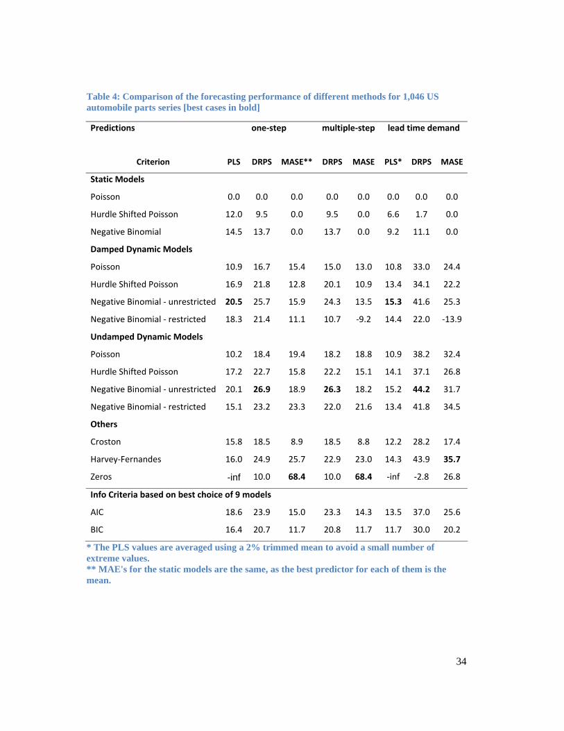
A summary of the results, in terms of percent improvements, is reported in Table 4. In all
cases larger values are better. A summary using medians instead of averages was also
produced but they were found to lead to similar conclusions and so are not reported here.
The summary for the PLS of lead-time demand was based on a trimmed mean to avoid
distortions from a few extreme cases. The zeros prediction method has Pr( 0) 1Y = = and
0P ( 0,r )Y ≠ = so its PLS results are reported as minus infinity.
Table 4 about here
A number of interesting observations can be made. First, the results in Table 4 are
reasonably consistent across the different types of forecasts. Second, the PLS and the
DRPS results suggest that the traditional static Poisson distribution can be too restrictive
for intermittent inventories. They confirm that better predictions may be obtained from
distributions which allow for over-dispersion, the negative binomial distribution being the
best option. This outcome was to be expected because the negative binomial distribution
has been widely used in inventory control for slow moving items, presumably because it
has been found to work in practice. Interestingly, the MASE and similar measures based
on point predictions, fail to reflect this important conclusion. They imply that the zero
prediction is best for one-step and multi-step predictions, which would result in zero safety
stocks for all items!
The main aim of this study was to assess methods that allow for serial correlation through
the use of dynamic specifications. The performance measures all indicate that there is a
significant improvement and the PLS and DRPS are reasonably consistent in their
rankings. Each measure indicates that the unrestricted negative binomial distribution is
best, although there is no clear indication of whether damped or undamped dynamics
should be used. The difference between both forms of dynamics is small according to both
criteria. Undamped dynamics gets our vote because it has strong links with the widely
used simple exponential smoothing forecasting method and because it has been found that
most business and economic time series are not stationary. Further, fewer parameters need
to be estimated which is important when series are short. However, as indicated in Section
3.4, there is an inconvenient aspect to this choice: simulated series values eventually
converge to a fixed point of zero.
Page 21
21
One interesting finding is that the Harvey-Fernandes method out-performed the widely
used Croston method of forecasting, or at least our adaption of it that allows for maximum
likelihood estimation of its parameters. It was shown in Section 3.2.1 that the Harvey-
Fernandes method has a limiting form corresponding to our restricted version of the
negative binomial model with undamped dynamics. Not surprisingly, both models had a
similar forecasting performance, the Harvey-Fernandes method having a slight edge.
However, the unrestricted version of the negative binomial model was markedly better
than both these approaches. What clearly emerges from this study is that, based upon the
PLS and DRPS criteria, our undamped negative binomial model significantly out-performs
both the adapted Croston method and the Harvey-Fernandes method.
The assumptions underlying the hurdle shifted Poisson distribution, as outlined in Section
3.1, appear to make it a strong candidate for intermittent demand forecasting. Yet, the
results from Table 4 indicate that its performance according to all the measures lags behind
the damped negative binomial model. In earlier numerical studies using the same data set,
a similar outcome (not reported here) was obtained for the zero-inflated Poisson
distribution.
The undamped hurdle shifted Poisson model is the closest model in our framework to the
modified Croston model. Instead of smoothing time gaps, we smooth the demand
occurrence indicator variable using equation (2). Interestingly, the undamped hurdle
shifted Poisson model does better than the adapted Croston method.
Multi-model approaches using information criteria for model selection were also explored
in the study. The methods designated as Others and the restricted versions of our negative
binomial models in Table 4 were excluded from the set of possible models for this part of
the project. Both the Akaike (AIC) and the Bayesian information criteria (BIC) were
considered. As might be expected, the AIC approach yielded the better forecasts on
average. Nevertheless, the unrestricted damped negative binomial case employed as an
encompassing model out-performed the multi-model approaches.
Tables 5 and 6 about here
The percentage breakdowns of the models selected by the AIC and BIC criteria are shown
in Tables 5 and 6. Static models proved to be quite adequate for about 60 percent of the
Page 22
22
series according to AIC and 77 percent according to the more stringent BIC criterion. We
need to keep in mind that the asymptotic justification for AIC is based upon forecasting
performance, whereas BIC is a consistent criterion for selecting the true model. Given the
forecasting focus of this study, AIC seems more appropriate. Moreover, no particular
distribution dominated. It is not clear how much emphasis should be placed on these
particular outcomes when the multi-model approach did not work as well as the
encompassing approach. Nevertheless, at first sight the prominence of static and Poisson
selections may be surprising. For those series, it is likely that all the models (except
‘zeros’) would perform well and AIC is simply guiding the modeler to the simpler scheme.
In the remaining cases the static or Poisson versions are inadequate and more complex
models are needed. With a different mix of series, the AIC may well outperform the
encompassing approach but it needs to be kept in mind that non-stationary models are
better able to adapt to structural changes in a series and may thus be preferable as an
‘insurance policy’.
There may be concern that our initial culling of the series has had a distorting effect on the
results. If all the series had have been included, the results for MASE and DRPS would
have shifted in the direction of the zeros method, the latter still having the value minus
infinity for PLS. In practice, items with such low levels of demand would often be covered
simply by placing special orders as needed.
7 Use of simulated demands in inventory control
Forecasts of demand, once they are obtained, can be fed into the decision processes for
inventory control. In this section we shall provide an example of how this can be done. A
more comprehensive exposition may be found in Hyndman et al. (2008, Chapter 18).
Our focus is on an SKU inventory, the demands for which are governed by a Poisson
distribution, the mean of which changes according to the undamped dynamic equation
underlying simple exponential smoothing, as defined in Tables 1 and 2. We assume that
the maximum likelihood estimate of the smoothing parameter α has been found using 55
months of data and is 0.1. It is now the beginning of month 56, a simple exponential
smoothing forecasting routine has yielded a point prediction for this month of 0.75, and a
replenishment order must be placed with a supplier. There is a delivery lead time of 2
Page 23
23
months, so any order placed now is not delivered until the beginning of month 58. The size
of the order is found by comparing the current total supply (current supply and outstanding
replenishment orders) with a pre-determined order-up-to level (OUL). The size of the
OUL determines the size of the order which in turn determines the level of service
provided to customers in month 58. The problem is to find a value for the OUL which
ensures that the expected fill rate in month 58 is at least 90 percent. Demands occurring
during shortages are backlogged.
The analysis begins by assigning a trial value to the OUL and determining the consequent
expected fill rate in month 58. Then we adjust the OUL until the expected fill rate equals
the target value of 90 percent. To begin, the analysis ignores the integer property of the
stock and treats the OUL as a continuous quantity. This search procedure is typically
automated by the use of a solver such as Goal-Seeker in Microsoft Excel.
Since predicted demand is 0.75 for each future month, as seen from the beginning of
month 56, and the extended lead time of interest is 2+1=3 months, we set the initial trial
value of the OUL equal to 3 X 0.75 which is 2.25. In other words, the initial trial value of
the OUL is set equal to mean extended lead time demand. There is no safety stock for this
initial situation.
We can then simulate future demands for months 56, 57 and 58 as shown in Table 7. The
first value of 0 was simulated from a Poisson distribution with a mean of 0.75. The mean
was revised in the light of this new simulated demand using simple exponential smoothing
to give a new mean of 0.675, this change being a reflection of presumed permanent
changes in the market for the inventory. The second value of 2 was simulated from a
Poisson distribution with a mean of 0.675. This procedure was again repeated (new mean
=0.8075), resulting in a simulated demand of 1 for month 58.
Given these three simulated future demands it is then possible to find the corresponding
sales in month 58, as shown in Table 8. The OUL represents the total stock available to
meet demand over the extended lead time of 3 months. After the OUL of 2.25 is used to
meet demands of 0 and 2 in months 56 and 57, month 58 begins with stock of 0.25. This is
insufficient to meet the simulated demand of 1 in month 48. Simulated sales immediately
Page 24
24
from stock can only be 0.25. The unsatisfied demand must be deferred until the next
delivery.
Insert Table 7 about here
This experiment can be repeated to create say 100 hypothetical future ensembles of
demand and sales in month 58. The ratio of the ensemble average of sales to the ensemble
average demand in month 58 can be viewed as an estimate of the fill-rate. This is unlikely
to exactly equal the target fill-rate with the initial trial value for the OUL. So, keeping the
demand scenarios unchanged, the OUL is adjusted by a solver until the estimated fill rate
equals the target value of 90 percent. The deviation of OUL from its initial value of the
mean extended lead time demand represents the safety stock. For practical reasons, any
resulting non-integer values of the OUL are rounded to the next highest integer, in which
case the target fill rate is usually exceeded.
Insert Table 8 about here
Regardless of which dynamic demand model is used, a simulation approach is needed
because the analytical form of future distributions of demands, as seen from the forecast
origin, are unknown, the exception being the distribution for the first future period.
Because of the associated computational loads, an approach like this would have been
completely impractical in the era when most of the basic ideas underpinning inventory
control theory were originally developed, ideas which still form the mainstay of most texts
on the subject. Analytical approaches were once a necessity for tractable computations, but
now the raw computational power provided by modern computers enables us to find
ordering parameters such as the OUL using approaches like the one described here in
under a second. Approaches like this are now feasible even for large numbers of SKUs.
8 Conclusions
In this paper we introduced some new models for forecasting intermittent demand time
series based on a variety of count probability distributions coupled with a variety of
dynamic specifications to account for potential serial correlation. These models were
Page 25
25
compared to established forecasting procedures using a database of car parts demands.
Particular emphasis was placed on prediction distributions rather than point forecasts from
these models because the latter ignores features such as variability and skewness which
can be important for safety stock determination.
The empirical results suggest that although many series may be adequately modeled using
traditional static schemes, substantial gains may be achieved by using dynamic versions
for many of the others. A similar argument favors the use of richer models than the
Poisson. Thus, an effective forecasting framework for SKUs that have low volume,
intermittent demands must look beyond the traditional static Poisson format.
Our study indicated that simple exponential smoothing can work well in conjunction with
an unrestricted negative binomial distribution. It also indicated that little advantage is
gained from using a multi-model approach with information criteria for model selection.
The usual caveat that such results are potentially data dependent must be made.
Nevertheless, it is our expectation that similar results would emerge for other datasets.
This being the case, it would appear that the Croston method, even in an adapted form,
should possibly be replaced by exponential smoothing coupled with a negative binomial
distribution.
There are a number of series, mostly excluded from the sample of 1,046 SKUs used here,
for which demand is very low, perhaps the order of one or two units per year. In such
cases, a static model might be preferable, although from the stock control perspective the
decision will often lie between holding one unit of stock or holding zero stock and
submitting special orders as needed.
There remains the important issue of what to do with new SKUs that have no or only
limited demand data. Then maximum likelihood methods applied to single series are going
to be ineffective. This is the subject of an on-going investigation into the forecasting of
demand for slow moving inventories where explore the possibility of extending the
maximum likelihood principle to multiple time series in a quest to overcome the paucity of
data.
Page 26
26
References
M. Akram, M., Hyndman, R.J. and Ord, J.K. (2009) Exponential smoothing and non-
negative data. Australia and New Zealand Journal of Statistics 51, 415 – 432.
Al-Osh M.A. and Alzaid, A.A. (1987) First-order integer valued autoregressive (INAR(1))
process. Journal of Time Series Analysis, 8, 261-275.
Billah, B., King, M.L., Snyder, R.D. and Koehler, A.B. (2006) Exponential smoothing
model selection for forecasting. International Journal of Forecasting, 22, 239 – 247.
Chatfield, C. (1992) Calculating interval forecasts. Journal of Business and Economic
Statistics, 11, 121-144.
Croston, J.D. (1972) Forecasting and stock control for intermittent demands. Operational
Research Quarterly, 23, 289-303.
Czado, C. Gneiting, T. and Held, L. (2009) Predictive model assessment for count data.
Biometrics, 65, 1254-1261.
Davis, R. A., Dunsmuir, W.T. and Wang, Y. (1999) Modelling time series of count data.
In Asymptotics, Nonparametrics & Time Series, Ed. S. Ghosh, pp 63-114. Marcel Dekker:
New York.
Davis, R.A., Dunsmuir, W.T.M, and Wang, Y. (2000) On autocorrelation in a Poisson
regression model. Biometrika, 87, 491-505
Durbin, J. and Koopman, S.J. (2001) Time Series Analysis by State Space Methods. Oxford
University Press: Oxford.
Eaves, A.H.C. and Kingsman, B.G. (2004) Forecasting for the ordering and stock-holding
of spare parts. Journal of the Operational Research Society 55, 431-437.
Epstein, E.S. (1969) A scoring system for probability forecasts of ranked categories.
Journal of Applied Meteorology, 8, 985-987.
Page 27
27
Feigin, P.D., Gould, P., Martin, G.M. and Snyder, R.D. (2008) Feasible parameter regions
for alternative discrete state space models. Statistics and Probability Letters 78 2963-2970.
Gardner, E.S. and Koehler, A.B. (2005) Comment on a patented bootstrapping method for
forecasting intermittent demand. International Journal of Forecasting, 21, 617-618.
Gneiting, T. and Raftery, A.E. (2007), Strictly proper scoring rules, prediction and
estimation, Journal of the American Statistical Association, 102, 359-378.
Grunwald, G.K., Hazma, K and Hyndman, R.J. (1997) Some properties and
generalizations of Bayesian time series models. Journal of the Royal Statistical Society, B
59, 615-626.
Harvey, A.C. and Fernandes, C. (1989) Time series models for count or qualitative
observations. Journal of Business and Economic Statistics, 7, 407-422.
Heinen, A. (2003) Modelling Time Series Count Data: An Autoregressive Conditional
Poisson Model. Working Paper, University of California, San Diego.
Hyndman, R.J. and Koehler, A.B. (2006) Another look at measures of forecast accuracy.
International Journal of Forecasting, 22, 679-688.
Hyndman, R.J., Koehler, A.B., Ord, J.K and Snyder, R.D. (2008) Forecasting with
Exponential Smoothing: The State Space Approach. Springer-Verlag: Berlin and
Heidelberg.
Johnson, N.L., Kotz, S. and Kemp, A.W. (1992) Univariate Discrete Distributions. Wiley:
New York. Second edition.
Johnston, F.R. and Boylan, J.E. (1996a) Forecasting for items with intermittent demand.
Journal of the Operational Research Society, 47, 113-121.
Johnston, F.R. and Boylan, J.E. (1996b) Forecasting intermittent demand: A comparative
evaluation of Croston’s method. Comment. International Journal of Forecasting, 12, 297-
298.
Page 28
28
Jung, R.C., Kukuk, M. and Leisenfeld, R. (2006) Time series of count data: modeling,
estimation and diagnostics. Computational Statistics and Data Analysis, 51, 2350-2364.
Makridakis, S. and Hibon, M. (2000). The M3-Competition: Results, conclusions and
implications. International Journal of Forecasting, 16, 451–476.
McCabe, B.P.M. and Martin, G.M. (2005) Bayesian predictions of low count time series.
International Journal of Forecasting, 21, 315-330.
McKenzie, E. (1988) Some ARMA models for dependent sequences of Poisson counts.
Advances in Applied Probability, 20, 822-835.
Murphy, A.H. (1971) A note on the ranked probability score. Journal of Applied
Meteorology, 10, 155-156.
Ord, J.K., Koehler, A.B. and Snyder, R.D. (1997) Estimation and prediction of a class of
dynamic nonlinear statistical models. Journal of the American Statistical Association, 92,
1621-1629.
Ord, J. K, Snyder, R.D. and Beaumont, A. (2010), Forecasting for Intermittent Demand
for Slow-Moving Items, Department of Econometrics and Business Statistics, Monash
University Working Paper 12/10.
Rao, A.V. (1973) A comment on: Forecasting and stock control for intermittent demands.
Operational Research Quarterly, 24, 639-640.
M. H. Quenouille (1949), A Relation between the logarithmic, Poisson, and negative
binomial series. Biometrics, 5, 162-164.
Sani, B. and Kingsman, B.G. (1997) Selecting the best periodic inventory control and
demand forecasting methods for low demand items. Journal of the Operational Research
Society, 48, 700-713.
Shenstone, L. and Hyndman, R.J. (2005) Stochastic models underlying Croston’s method
for intermittent demand forecasting. Journal of Forecasting, 24, 389-402.
Page 29
29
Shephard, N. (1995) Generalized Linear Autoregressions. Working Paper, Nuffield
College, Oxford.
Snyder, R.D. (2002) Forecasting sales of slow and fast moving inventories. European
Journal of Operational Research, 140, 684-699.
Snyder, R.D., Koehler, A.B. and Ord, J.K. (1999) Lead Time Demand for Simple
Exponential Smoothing: An Adjustment Factor for the Standard Deviation, Journal of the
Operational Research Society, 50, 1079-1082.
Stuart, A. and Ord, J.K. (1994) Kendall’s Advanced Theory of Statistics. London: Edward
Arnold. Sixth edition.
Syntetos, A.A. and Boylan, J.E. (2001) On the bias of intermittent demand estimates.
International Journal of Production Economics, 71, 457-466.
Syntetos, A.A. and Boylan, J.E. (2005) The accuracy of intermittent demand estimates.
International Journal of Forecasting, 21, 303-314.
Syntetos, A.A., Nikolopoulos, K. and Boylan, J.E.(2010) Judging the judges through
accuracy implication metrics: The case of inventory forecasting. International Journal of
Forecasting, 26, 134-143.
Teunter, R.H. and Duncan, L. (2009) Forecasting intermittent demand: a comparative
study. Journal of the Operational Research Society, 60, 321-329.
West, M, Harrison, J. Migon, H. S. (1985). Dynamic generalized models and Bayesian
forecasting (with discussion). Journal of the American Statistical Association, 80, 73-97.
West, M. and Harrison, J. (1997), Bayesian Forecasting and Dynamic Models, second
edition, Springer-Verlag, New York.
Willemain, T.R., Smart, C.N., Shockor, J.H. and DeSautels, P.A. (1994) Forecasting
intermittent demand in manufacturing: a comparative evaluation of Croston’s method.
International Journal of Forecasting, 10, 529-538.
Page 30
30
Willemain, T.R., Smart, C.N. and Schwartz, H.F. (2004) A new approach to intermittent
forecasting demand for service parts inventories. International Journal of Forecasting, 20,
375-387.
Winklemann, R. (2008) Econometric Analysis of Count Data, 5th edition, Springer-Verlag,
New York.
Zeger, S.L. (1988) A regression model for time series counts. Biometrika, 75, 621-629.
Page 31
31
Table 1 Count distributions used in the empirical study
Distribution Mass Function Parameter
Restrictions
Mean, µ
Poisson ( )exp
!
y
yλ λ−
0λ > λ
Negative
Binomial ( )( )
1! 1 1
a ya y ba y b b
Γ + ⎛ ⎞ ⎛ ⎞⎜ ⎟ ⎜ ⎟Γ + +⎝ ⎠ ⎝ ⎠
0, 0a b> > a
b
Hurdle Shifted
Poisson 1
0exp( ) / ( 1)! 1,2,y
q yp y yλ λ−
=⎧⎨ − − = …⎩
0, 0,0, 1
p qp qλ
≥ >> + =
( 1)p λ +
Notes: When the iterative estimation procedure generated an estimated value of b that exceeded 99, the negative binomial was replaced by the Poisson distribution. Typically this condition was the result of under-dispersion, which would lead to the Poisson as a limiting case. The negative binomial form was chosen for consistency with the Harvey-Fernandes version, rather than the more orthodox version with / (1 ).p b b= +
Page 32
32
Table 2: Recurrence relationships for the mean
Relationship Recurrence Relationship
Restrictions
Static 1t tμ μ −=
Damped dynamic 1 1t t tc yμ φμ α− −= + + 0, 0, 01
c φ αφ α> > >+ <
Undamped dynamic 1 1t t tyμ δμ α− −= + 0, 01
δ αδ α> >+ =
Page 33
33
Table 3: Conversion of latent factors to distribution parameters
Distribution Formula
Poisson t tλ μ=
Negative Binomial t ta bμ=
Hurdle Shifted Poisson 1tt
tpμλ = −
Page 34
34
Table 4: Comparison of the forecasting performance of different methods for 1,046 US automobile parts series [best cases in bold]
Predictions one‐step multiple‐step lead time demand
Criterion PLS DRPS MASE** DRPS MASE PLS* DRPS MASE
Static Models
Poisson 0.0 0.0 0.0 0.0 0.0 0.0 0.0 0.0
Hurdle Shifted Poisson 12.0 9.5 0.0 9.5 0.0 6.6 1.7 0.0
Negative Binomial 14.5 13.7 0.0 13.7 0.0 9.2 11.1 0.0
Damped Dynamic Models
Poisson 10.9 16.7 15.4 15.0 13.0 10.8 33.0 24.4
Hurdle Shifted Poisson 16.9 21.8 12.8 20.1 10.9 13.4 34.1 22.2
Negative Binomial ‐ unrestricted 20.5 25.7 15.9 24.3 13.5 15.3 41.6 25.3
Negative Binomial ‐ restricted 18.3 21.4 11.1 10.7 ‐9.2 14.4 22.0 ‐13.9
Undamped Dynamic Models
Poisson 10.2 18.4 19.4 18.2 18.8 10.9 38.2 32.4
Hurdle Shifted Poisson 17.2 22.7 15.8 22.2 15.1 14.1 37.1 26.8
Negative Binomial ‐ unrestricted 20.1 26.9 18.9 26.3 18.2 15.2 44.2 31.7
Negative Binomial ‐ restricted 15.1 23.2 23.3 22.0 21.6 13.4 41.8 34.5
Others
Croston 15.8 18.5 8.9 18.5 8.8 12.2 28.2 17.4
Harvey‐Fernandes 16.0 24.9 25.7 22.9 23.0 14.3 43.9 35.7
Zeros -inf 10.0 68.4 10.0 68.4 ‐inf ‐2.8 26.8
Info Criteria based on best choice of 9 models
AIC 18.6 23.9 15.0 23.3 14.3 13.5 37.0 25.6
BIC 16.4 20.7 11.7 20.8 11.7 11.7 30.0 20.2
* The PLS values are averaged using a 2% trimmed mean to avoid a small number of extreme values. ** MAE's for the static models are the same, as the best predictor for each of them is the mean.
Page 35
35
Table 5: Percentage breakdown of AIC model selections
Dynamics Distribution Static Damped Undamped TotalPoisson 15 18 1 34 Negative binomial 21 11 4 36 Hurdle Poisson 24 5 0 30 Total 60 34 6 100
Page 36
36
Table 6: Percentage breakdown of BIC model selections
Dynamics Distribution Static Damped Undamped TotalPoisson 31 10 5 46 Negative binomial 24 2 5 31 Hurdle Poisson 22 0 0 23 Total 77 13 10 100
Page 37
37
Table 7 Simulation of Future Demands from Undamped Dynamic Poisson Model
Period
Point Prediction
(Mean) Simulated Demand
56 0.75 0 57 0.675 2 58 0.8075 1
Page 38
38
Table 8 Sales calculation from simulated demands
Period Variable Value
56 Order-Up-To Level 2.25
Trial value specified by user (OUL)
56 Demand 0 Simulated demand (D56) 57 Demand 2 Simulated demand (D57) 58 Open Stock 0.25 max(OUL-D56-D57,0) 58 Demand 1 Simulated demand (D58) 58 Sales 0.25 min(Open Stock, D58)