Foreign Currency Loans and Credit Risk: Evidence from U.S. Banks * Friederike Niepmann and Tim Schmidt-Eisenlohr † September 19, 2017 Abstract When firms borrow in foreign currency but collect revenues in local currency, exchange rate changes can affect their ability to repay their debt. Using loan-level data from U.S. banks’ regulatory filings, this paper studies the effect of exchange rate changes on firms’ loan payments. A 10 percent depreciation of the local currency makes a firm with foreign currency debt 69 basis points more likely to become past due on its loans than a firm with local currency debt. This result implies that firms do not perfectly hedge against exchange rate risk and that this risk translates into credit risk for banks. The findings lend support to both the balance sheet channel and the financial channel of exchange rates. Keywords : cross-border banking, exchange rates, credit risk, corporate loans JEL-Codes : F31, G15, G21 * The authors are grateful to Mark Carey, Ricardo Correa, Wenxin Du, Caroline Pflueger, and Jesse Schreger for helpful comments as well as participants in the Board’s IFS Lunch Workshop. The authors also thank Tyler Bodine-Smith, Patrick Russo, Elizabeth Doppelt, Stefan Walz, and Beau Bressler for excellent research assistance. † The authors are staff economists in the Division of International Finance, Board of Governors of the Federal Reserve System, Constitution Avenue NW, Washington, D.C. 20551, USA. Emails: [email protected]and [email protected]. The views in this paper are solely the responsibility of the authors and should not be interpreted as reflecting the views of the Board of Governors of the Federal Reserve System or of any other person associated with the Federal Reserve System.
Transcript
Foreign Currency Loans and Credit Risk:
Evidence from U.S. Banks*
Friederike Niepmann and Tim Schmidt-Eisenlohr†
September 19, 2017
Abstract
When firms borrow in foreign currency but collect revenues in local currency, exchange
rate changes can affect their ability to repay their debt. Using loan-level data from U.S.
banks’ regulatory filings, this paper studies the effect of exchange rate changes on firms’
loan payments. A 10 percent depreciation of the local currency makes a firm with foreign
currency debt 69 basis points more likely to become past due on its loans than a firm with
local currency debt. This result implies that firms do not perfectly hedge against exchange
rate risk and that this risk translates into credit risk for banks. The findings lend support
to both the balance sheet channel and the financial channel of exchange rates.
*The authors are grateful to Mark Carey, Ricardo Correa, Wenxin Du, Caroline Pflueger, and Jesse Schreger
for helpful comments as well as participants in the Board’s IFS Lunch Workshop. The authors also thank Tyler
Bodine-Smith, Patrick Russo, Elizabeth Doppelt, Stefan Walz, and Beau Bressler for excellent research assistance.†The authors are staff economists in the Division of International Finance, Board of Governors of the Federal
and [email protected]. The views in this paper are solely the responsibility of the authors and
should not be interpreted as reflecting the views of the Board of Governors of the Federal Reserve System or of
any other person associated with the Federal Reserve System.
1 Introduction
Borrowing in foreign currency is a prevalent phenomenon, especially in emerging market economies.
While loans denominated in a foreign currency are typically cheaper than domestic currency
loans, they expose firms to exchange rate risk. Financial markets offer instruments to hedge
against this risk, but these instruments are costly, and firms often remain unhedged.1 In this
case, when the domestic currency depreciates, firms’ debt burden increases with negative conse-
quences for their economic performance (the so-called balance sheet channel).
Traditionally, currency devaluations have been thought of as enhancing firm performance
by increasing the foreign demand for domestic goods. However, because of the balance sheet
channel, devaluations can be contractionary (Bebczuk et al. (2010) and Kohn et al. (2015)),
cause or worsen currency crises (Aghion et al. (2001), Aghion et al. (2004), Ranciere et al.
(2010a)), and create systemic risk (Dell’Ariccia et al. (2016b) and Yesin (2013)). In addition,
they may feed back onto bank balance sheets through higher credit risk, causing a reduction in
cross-border lending (Bruno and Shin (2014) and Avdjiev et al. (2016)).2
Understanding the aggregate effects of exchange rate changes is highly relevant to policy
makers because exchange rates often respond to policy decisions; they can be a channel for
international spillovers of both monetary policy (Eichenbaum and Evans (1995) and Cushman
and Zha (1997)) and fiscal policy (Kim and Roubini (2008) and Corsetti and Muller (2006)).
For example, a divergence of the monetary policy stances of the United States and the euro
area may cause the USD to appreciate. Also, a destination-based cash flow tax (DBCFT) with a
border adjustment, which has been discussed in the United States, would likely lead to significant
USD appreciation, raising concerns about adverse effects on borrowers, especially in emerging
markets.3
Micro-level evidence on the relevance of the balance sheet channel is limited and mixed. Most
studies in the literature rely on firm balance sheet data from a small set of countries to study
this question. Aguiar (2005) uses Mexican balance sheet data, finding that firms with heavy
short-term foreign debt exposure had substantially lower investments after a large devaluation.
Along these lines, Kim et al. (2015) report that firms’ economic performance declined more
for firms with foreign currency debt during the 1997-1998 Korean crisis. In contrast, Bleakley
and Cowan (2008) do not find such differential effects, using accounting data for five Latin
American countries. Kalemli-Ozcan et al. (2016) document adverse effects of devaluations on firm
investment in the presence of foreign-denominated debt but only if there is a contemporaneous
banking crisis.
Using unique loan-level data derived from U.S. banks’ regulatory filings, this paper provides
1On the trade-offs involved in hedging, see, for example, Nance et al. (1993) and Geczy et al. (1997).2See also Eichengreen et al. (2007) for a general discussion of currency mismatch.3See Auerbach et al. (2017) for a discussion of the DBCFT.
1
direct evidence on the balance sheet channel. Specifically, we show that exchange rate changes
affect firms’ ability to service their debt when the firms’ debt is denominated in a foreign currency.
This study contributes to the existing literature in three distinct ways. First, it documents
the relevance of the balance sheet channel in normal times based on a sample of firms in 105
countries. As mentioned, previous papers have mainly focused on a single country or a small set
of countries during large devaluations. Second, the detailed loan-level data with broad country
coverage allow for a robust estimation with a large number of fixed effects. Third, because the
data are derived from bank loan portfolios, this paper provides the first direct evidence that
exchange rate fluctuations (exchange rate risk) translate into credit losses (credit risk) for banks.
The loan-level data come from Y-14 filings that banks subject to stress testing by the Federal
Reserve have to file on a quarterly basis. They are composed of corporate loans and leases with
a loan amount of at least $1 million and contain various characteristics of the loans, including
whether and how long they have been past due. We also observe the location of the borrower
and the currency denomination of the loan as well as loan size, maturity, and the interest rate,
among other characteristics. Importantly, 84 percent of the loans are not syndicated, meaning
that the majority of loans in our dataset cannot be found in syndicated loan databases, which
are often the data source of choice for cross-country loan-level studies. The sample period runs
from 2014q4 to 2016q2, a period of substantial USD appreciation.
Before exploring the balance sheet channel, we establish several facts. First, as of 2016q2, 75
percent of loans to non-U.S. residents are denominated in a different currency than the borrower’s
home currency. Second, only a small share of loans is ever past due, roughly 0.6 percent of loans.
Third, foreign currency loans are around 151 basis points cheaper. Fourth, foreign currency loans
are more prevalent in countries with higher inflation, lower exchange rate volatility, and a higher
credit-to-GDP ratio. Also, firms in industries with a higher share of foreign sales and a lower
share of foreign assets are more likely to borrow a foreign currency. Finally, foreign currency
loans are larger and of shorter maturity.
A key challenge in identifying the balance sheet channel is that exchange rates are correlated
with macroeconomic variables that also drive firm performance. Testing for the balance sheet
channel therefore requires isolating it from other confounding channels. We do this by comparing
firms with foreign debt with firms with domestic debt in the same country, industry, quarter,
and with the same bank-internal rating. Furthermore, we control for the size of loans and
their maturities. Our identification assumption is that, in the absence of foreign currency debt,
exchange rate changes would affect firms in the same industry, country, and quarter and with
the same bank-internal rating, loan size and maturity structure in the same way. Obviously, a
firm’s choice of currency is not random, and it is challenging to control for all possible factors.
But the key is that the selection of firms into currency happens in a way that makes it less likely
for us to find effects of exchange rate changes on loan payments. Firms tend to choose foreign
currency debt when they have foreign income or foreign assets (Brown et al. (2011), Bleakley
2
and Cowan (2008), Kedia and Mozumdar (2003), and Keloharju and Niskanen (2001)).4 And
in the absence of natural hedges, firms with larger foreign currency exposures are more likely to
buy protection against currency moves (for example, Geczy et al. (1997)). Also, banks have an
incentive to lend in foreign currency to firms that better tolerate exchange rate volatility.
Nevertheless, we find strong evidence that exchange rate movements affect firms’ ability
to service their debt, which indicates that firms remain significantly exposed to exchange rate
volatility. A 10 percent depreciation of the local currency increases the probability that a firm
becomes past due on its loans by 69 to 160 basis points more for firms with foreign currency debt
compared with firms with domestic currency debt. This effect mainly stems from local currency
depreciations and is stronger for firms in industries with a smaller share of foreign sales. Applying
these results to the total foreign currency loans of U.S. banks in our sample indicates that a 10
percent appreciation of the USD causes an increase in late loan payments of $2.5 billion for these
banks.
More related literature A considerable number of papers study the balance sheet channel
using macro and micro data. Starting with macro-level evidence, Edward (1986) finds short-term
contractionary effects of devaluations. Cespedes (2005) shows that devaluations have stronger
negative effects on output for countries that are more indebted. Bebczuk et al. (2010) analyze the
role of dollar denominated debt for the effect of real depreciations on GDP growth, documenting
that dollar debt can make devaluations contractionary.5 Studies using micro-level data have
analyzed the effect of foreign currency debt on firm investment and employment with mixed
evidence on the balance sheet channel, as mentioned before. Similar to Aguiar (2005), Carranza
et al. (2003), Echeverry et al. (2003), Benavente et al. (2003), and Galiani et al. (2003) find that
firms with higher foreign debt contract investment more after devaluations. Based on data from
Hungary, Varela and Salomao (2016) find that foreign currency borrowing is associated with
higher aggregate income, but at the expense of higher volatility.
The link between exchange rate changes and credit risk has been emphasized by macro-
oriented papers studying the causes of financial crises, but less so in the banking literature.
Bozovic et al. (2009) provide a model where exchange rate risk spills over into default risk,
resulting in reduced credit supply and growth. Bruno and Shin (2015) focus on the implications
of local currency depreciation and increased credit risk for global banks and these banks’ cross-
border lending.6
4See also Kamil (2012) and Brown et al. (2014a). See Galindo et al. (2003a) for a survey on the determinantsof debt currency denomination.
5In addition, see Kamin and Klau (1997).6Two recent papers investigate whether banks charge higher interest on loans when firms have foreign currency
exposures. See Francis and Hunter (n.d.) and Kim et al. (2016).
3
2 Background on Foreign Currency Debt
When a firm borrows in a foreign currency but its revenues are in local currency, this currency
mismatch can affect its performance. Without hedging through foreign exchange swaps or natural
hedges (that is, revenues in foreign currency), the firm faces a higher debt burden when the
local currency depreciates. In response, firms might lower their investment, reduce staff and,
ultimately, become unable to service their debt.7 The following section provides more background
information and summarizes evidence in the literature on foreign currency borrowing and the
balance sheet channel.
Foreign currency debt is a relevant phenomenon. It is especially prevalent in emerging
economies. Figure 1 illustrates this fact using data from the Bank for International Settlements
(BIS) on cross-border banking. Total cross-border borrowing from banks in BIS reporting coun-
tries by 67 borrowing countries was just below $18 trillion at the end of the second quarter of
2016. Figure 1 shows the share of cross-border borrowing denominated in foreign currency from
2012 to 2017, dividing countries into emerging and advanced economies.8 More than 70 percent
of funds borrowed cross-border from foreign banks by emerging countries are denominated in one
of the five major currencies. In contrast, less than 40 percent of funds borrowed by advanced
economies are denominated in a foreign currency. The dataset employed in this paper, which is
composed of U.S. banks’ corporate loans to non-U.S. residents, reveals a similar pattern, with
75 percent of loans denominated in a foreign currency in the second quarter of 2016.
Why do firms borrow in a foreign currency instead of the local currency? Foreign
currency loans may be cheaper than local currency loans. The U.S. bank-level data show that
foreign currency loans are in fact associated with lower interest rates during the 2014-2016 time
period, which the dataset derived from Y-14 data used in this paper covers. Table 1 shows a
regression of the interest rate of a loan on a dummy that is one when the loan is denominated in
a foreign currency controlling for a battery of fixed effects and additional variables. On average,
the interest rate on foreign currency loans is 151 basis points lower than on local currency loans,
as shown in column 5 of the table. The column displays the results when firm-time, loan-type,
and interest-rate-type fixed effects are included in the regression.
A second reason for foreign currency borrowing is firms’ desire to hedge against currency
risk arising from income in foreign currency or assets denominated in foreign currency. For
example, Brown et al. (2009) report that foreign currency income is the dominant reason for
foreign currency borrowing in Eastern Europe. Similarly, Bleakley and Cowan (2008), Kedia and
7For theoretical papers that model the balance sheet channel, see Jeanne (2000), Aghion et al. (2001), Caballeroand Krishnamurthy (2003), Ranciere et al. (2008), Kohn et al. (2015), and Dell’Ariccia et al. (2016a).
8The shares shown are lower bounds. The BIS Locational Statistics leave a portion of the cross-borderborrowing unallocated for countries that do not have the EUR, CHF, GBR, JYE, USD as the domestic currency.
4
Figure 1: Share of cross-border borrowing from banks denominated in foreign currency
Note: The chart is based on the Locational Banking Statistics maintained by the Bank for International Set-tlements. It shows the cross-border borrowing from banks in BIS reporting countries in a currency other thanthe borrowing country’s home currency as a share of total cross-border bank borrowing for two groups of coun-tries: 30 emerging economies and 27 advanced economies. For the emerging economies foreign borrowing includesborrowing in GBP, JPY, USD, EUR, and CHF.
5
Table 1: Interest rates on local currency versus foreign currency loans
(0.000532) (0.000514) (0.000755) (0.000751)Time FE Yes No No No NoCt-time FE No Yes No No NoFirm-time FE No No Yes Yes YesLoan type FE No No No Yes YesRate type FE No No No No YesObservations 11566 11405 3811 3178 3178𝑅2 0.057 0.320 0.885 0.898 0.899
Note: This table shows results of regressions of a loan’s interest rate on a dummy variable that takes a value of1 if the loan is denominated in a foreign currency. Other regressors are the loan’s log loan size and log maturity.Column 1 includes time fixed effects, column 2 country-time fixed effects, column 3 firm-time fixed effects, andcolumn 4 firm-time plus loan-type fixed effects. Finally, column 5 adds fixed effects for the type of interest rategrouped into variable-, floating- and mixed-rate loans. Standard errors are clustered by bank-quarter. *, ** and*** denote significance at the 10%, 5% and 1% level.
Mozumdar (2003), and Keloharju and Niskanen (2001) find that firms obtain foreign currency
debt to hedge against foreign currency income.9 Additional evidence suggests that banks also
influence the denomination of loans. Brown et al. (2014b) show that “foreign currency lending
is at least partially driven by bank eagerness to match the currency structure of assets with that
of liabilities,” indicating that supply factors can also play a role.
When does foreign currency debt give rise to a balance sheet channel? Several condi-
tions have to be met. First, foreign currency borrowing must lead to a currency mismatch. This
happens when firms are not hedged. As discussed above, firms with foreign currency loans often
have natural hedges. And even if they are not naturally hedged, they can buy protection against
local currency depreciation and engage in foreign exchange swaps.10 However, not all firms may
hedge because it is costly. While data on the foreign currency exposure of firms is generally
scarce, the literature agrees that currency mismatch is an issue and has played a significant role
in past crises. Currency mismatch is thought to have been a key amplifier during the Asian crisis
in the late 90s (for example, Corsetti et al. (1999)). Moreover, currency mismatch in Eastern
Europe has been documented and discussed as a source of systemic risk, for example by Ranciere
9For literature reviews, see Kamil (2012) and Galindo et al. (2003b).10Geczy et al. (1997) show that firms with foreign exchange rate exposures are more likely to use currency
derivatives.
6
et al. (2010b) and Yesin (2013).
A second condition for the balance sheet channel to operate relates to firms’ responses to a
higher debt burden. If firms have a currency mismatch and debt servicing costs rise because
the local currency depreciates, firms could pass on the higher cost to their customers through
higher prices. However, firms might not be able to increases prices either because of the market
structure and competitive pressures or because prices are sticky in the short-run. As the local
exchange rate depreciates, the cost of debt for these firms, which often face monthly interest
payments, rises but prices cannot be adjusted promptly to compensate the firms for the higher
cost. A large literature documents short-term price stickiness and less than perfect pass-through
of higher costs to consumers. (See, for example, Klenow and Kryvtsov (2008), Klenow and Malin
(2010), Nakamura and Steinsson (2013), and Gopinath and Rigobon (2008)).
3 The Dataset
3.1 The Data Source for Corporate Loans
The loan-level data used in this paper come from Y-14 reports that U.S. banks that are stress-
tested by the Federal Reserve have to file on a quarterly basis.11 Banks report corporate loans
that are held for investment and held for sale with a committed exposure above $1 million.
They report at the consolidated level, that is, we observe not only cross-border loans extended
to foreign firms by the parent bank but also those extended by the banks’ foreign subsidiaries
and branches (although we cannot distinguish them). Reporting of the loan-level information
started in 2011q3. However, information of the currency denomination of the loan, crucial for
our analysis, is only available from 2014q4 onwards. Therefore, the baseline sample covers a
smaller time period, running from 2014q4 to 2016q2. During this time, the dollar appreciated
significantly, as figure 2 illustrates. The sample includes 31 different banks. Some banks enter
the sample as they become part of the annual stress-testing exercise.
To obtain a consistent dataset, we subject the data to several cleaning procedures and collapse
the loan-level dataset to the borrower level.12 A borrower is identified as a combination of cus-
tomer identifier, location, and bank name.13 The least restrictive sample has 74,747 observations
and covers 19,210 borrowers residing in 105 different countries.14
11Banks report corporate loans on schedule H.1. The data are confidential but available to researchers withinthe Federal Reserve System.
12While borrowers may decide to delay payments on individual loans, the decision is taken at the borrower-level,making it the appropriate level for our analysis. Indeed, in our data, in almost all cases, borrowers are late withtheir payments on all of their loans at the same time.
13In general, when collapsing the data, we calculate utilized exposure-weighted averages for all variables. Detailson data cleaning can be found in the data appendix.
14We drop countries whose currencies are pegged to the USD.
7
Figure 2: USD index, 2011q3 to 2016q2
Note: This figure shows the USD broad index, an index of the trade-weighted USD exchange rate against a basketof currencies calculated by Federal Reserve Board staff. The period shown goes from 2011q3 to 2016q2.
3.2 Dataset Facts
A significant portion of the loans is in non-local currencies. 50 percent of firm-quarter
observations in the dataset borrow exclusively in USD. In contrast, 41 percent obtain loans in
their local currency only. 4.5 percent take loans in a foreign currency other than the USD. And
5.5 percent of firms borrow in a variety of currencies. Table 2 shows the average and median
loan size, maturity, probability of default and interest rate of lending in different currencies. As
the table highlights, firms that only borrow in foreign currency take out larger loans than firms
that borrow in the local currency. Firms that borrow in multiple currencies have the largest
loan volumes, likely because they are larger. The median maturity of the loans is between 4.3
and 5 years. Local currency loans carry a higher interest rate than foreign currency loans, as
also formally established in table 1, and have a slightly higher probability of default. Additional
details on foreign versus local currency loans are discussed in section 4.2.
The majority of loans is not syndicated or participated. A large number of papers in
the literature analyze syndicated loans. Information on these loans is available from commercial
sources and has been collected for many years. While the loan-level data obtained from banks’
Y-14 reports is only available for a relatively short time period, they have the advantage of
8
Table 2: Loan characteristics, by currency
(1) (2) (3) (4)USD oth foreign local mix
mean p50 mean p50 mean p50 mean p50util. exposure ($m) 30.8 7.71 29.1 5.64 14.9 3.67 64.8 27.7maturity (years) 5.79 4.53 5.61 4.70 4.93 4.32 6.19 5.00prob. of default (pct) 2.28 0.68 1.76 0.64 2.42 0.71 2.08 0.71interest rate (pct) 2.92 2.07 3.03 2.34 4.27 3.82 3.53 2.76loans newly past due (pct) 0.41 0 0.42 0 0.27 0 0.22 0loans past due (pct) 0.64 0 0.63 0 0.54 0 0.47 0Observations 37019 3339 30313 4076Share of obs. (pct) 49.5 4.5 40.6 5.5
Note: The table shows summary statistics of the baseline sample with 74,747 observations grouped by the currencydenomination of loans. Column 1 includes observations where the borrower has loans denominated exclusivelyin USD. Column 2 has observations where the borrowers has loans in a foreign currency other than the USD.Column 3 is based on borrowers with local currency loans. Column 4 includes observations where the borrowershas loans in multiple currencies. The table displays the means and the medians of the following variables: utilizedexposure, maturity, bank-internal probability of default, interest rate, a dummy variable which is one when theborrower becomes past due on (some of) its loans, and a dummy variable which is one when the borrower is pastdue on any of its loans in period 𝑡.
including a larger set of loans as table 3 points out. 84 percent of the observations in the sample
are not syndicated. The average size of these loans is less than half of that of syndicated loans.
Moreover, they have a slightly lower average maturity and carry higher interest. Interestingly, a
similar share of loans in both groups is in local versus foreign currencies.15
The event that a borrower does not service its debt is rare. The Y-14 reports contain
information on whether borrowers are late on their interest or principal payments, information
which forms the basis of our analysis. Only a small fraction of borrowers is ever late on their
loan payments: 0.6 percent of observations are associated with late payment status. For the
regression analysis, we construct a variable that takes the value of 1 if a borrower becomes late
on its loan payments in a given quarter. The event that a borrower misses a loan or principal
payment for the first time is very rare and happens 255 times in our dataset. Tables 2 and 3
show the percentage of observations that have past due or new past due status split by currency
and participation type. Of note, even though local currency loans have higher probabilities of
default, which measure the banks’ ex-ante assessment of their riskiness, they become less often
past due than foreign currency and USD loans, i.e. they are ex-post less risky over the sample
period. The fact that foreign currency loans turned out to be riskier than anticipated by banks
might be a result of the unanticipated appreciation of the USD over that period. That is, based
15Around 2 percent of borrowers have a mix of syndicated and non-syndicated loans. In this table, borrowerswith less than 50 percent of syndicated loans are classified as not syndicated.
9
Table 3: Loan characteristics, syndicated vs. non-syndicated
(1) (2)non-syndicated syndicatedmean p50 mean p50
util. exposure ($m) 21.7 4.59 48.6 24.8maturity (years) 5.35 4.09 5.97 5.01prob. of default (pct) 2.17 0.71 2.97 0.64interest rate (pct) 3.66 2.98 2.72 2.33loans newly past due (pct) 0.37 0 0.21 0loans past due (pct) 0.57 0 0.66 0loans in for. currency (pct) 0.57 1 0.61 1Observations 62439 12308Share of obs. (pct) 83.5 16.5
Note: The table shows summary statistics of the baseline sample with 74,747 observations grouped into syndicatedand non-syndicated loans. Column 1 includes observations where less than 50 percent of the borrower’s loansare syndicated. Column 2 has observations where at least 50 percent of the borrower’s loans are syndicatedor participated. The table displays the means and the medians of the following variables: utilized exposure,maturity, bank-internal probability of default, interest rate, a dummy variable which is one when the borrowerbecomes past due on (some of) its loans, a dummy variable which is one when the borrower is past due on any ofits loans in period 𝑡, and the share of a borrower’s loans that are not denominated in the currency of the countrywhere the borrower is located.
on our results, the appreciation made foreign currency loans relatively more risky than domestic
currency loans ex-post.
The dataset covers loans in a variety of countries and industries. The 105 countries
in the sample span various world regions. Table 4 shows loan characteristics by region. The
largest share of the loans goes to high-income OECD countries, followed by countries in Latin
America and the Caribbean. Borrowing in foreign currency is particularly prevalent in Europe
and Central Asia, Latin America and the Caribbean, and Sub-Saharan Africa.
Table 5 displays loan characteristics by industry. 34 percent of observations belong to manu-
facturing firms. 18 percent belong to the the finance and insurance industry. 14 percent each are
in other service industries and in wholesale and retail trade. Loans in the finance and insurance
sector are significantly larger and carry lower risk and interest compared to other industries.
The event that a borrower becomes past due on its loan payments is relatively evenly distributed
across regions and industries.
3.3 Additional Data Sources
The borrower-level dataset is complemented with several variables that come from a variety of
sources. Information on bilateral exchange rates are from the IMF’s International Financial
Time FE Yes Yes Yes Yes Yes NoCt-Time-Ind-Rat No No No No No YesObservations 7594 8250 11128 11645 6092 3513Pseudo 𝑅2 0.071 0.021 0.001 0.026 0.103 0.182
Note: This table explores the characteristics of foreign currency versus local currency loans. A dummy that takesa value of 1 if the loan is in foreign currency is regressed on macro variables (column 1), industry- (column 2),firm- (column 3), and loan-level characteristics (column 4). Column 5 includes all explanatory variables. Column6, includes country-time-industry-rating fixed effects, in contrast to the other columns that include time fixedeffects. Standard errors are clustered by country-time (columns 1, 5, and 7), industry-country (column 2), andfirm (columns 3 and 4). *, ** and *** denote significance at the 10%, 5% and 1% level.
macroeconomic and industry variation is now fully absorbed by the fixed effects. Also the rating
is now directly controlled for. The two remaining factors that are not absorbed by the extensive
fixed effects, loan size and maturity, however, remain significant predictors of currency choice.
4.3 Evidence on the Balance Sheet Channel
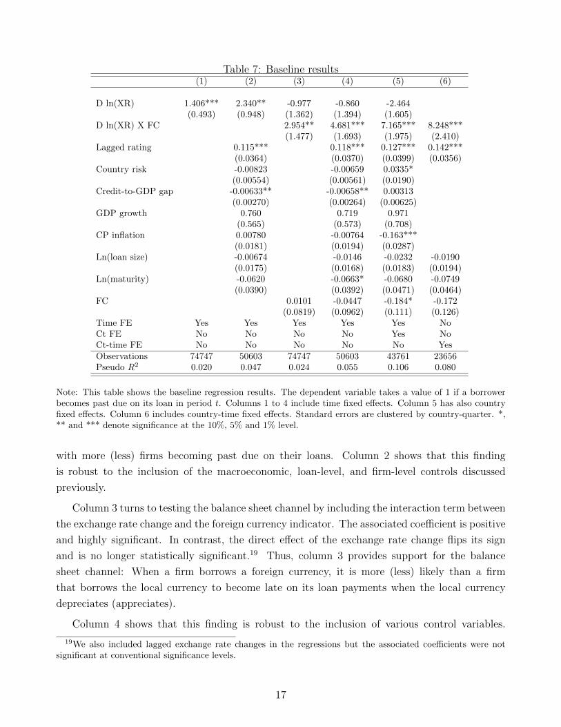
This section presents our main findings on the balance sheet channel. Table 7 displays the
baseline results.
Baseline results Column 1 shows that exchange rate changes are positively correlated with
firms’ payment status; that is, a depreciation (appreciation) of the local currency is associated
FC 0.0101 -0.0447 -0.184* -0.172(0.0819) (0.0962) (0.111) (0.126)
Time FE Yes Yes Yes Yes Yes NoCt FE No No No No Yes NoCt-time FE No No No No No YesObservations 74747 50603 74747 50603 43761 23656Pseudo 𝑅2 0.020 0.047 0.024 0.055 0.106 0.080
Note: This table shows the baseline regression results. The dependent variable takes a value of 1 if a borrowerbecomes past due on its loan in period 𝑡. Columns 1 to 4 include time fixed effects. Column 5 has also countryfixed effects. Column 6 includes country-time fixed effects. Standard errors are clustered by country-quarter. *,** and *** denote significance at the 10%, 5% and 1% level.
with more (less) firms becoming past due on their loans. Column 2 shows that this finding
is robust to the inclusion of the macroeconomic, loan-level, and firm-level controls discussed
previously.
Column 3 turns to testing the balance sheet channel by including the interaction term between
the exchange rate change and the foreign currency indicator. The associated coefficient is positive
and highly significant. In contrast, the direct effect of the exchange rate change flips its sign
and is no longer statistically significant.19 Thus, column 3 provides support for the balance
sheet channel: When a firm borrows a foreign currency, it is more (less) likely than a firm
that borrows the local currency to become late on its loan payments when the local currency
depreciates (appreciates).
Column 4 shows that this finding is robust to the inclusion of various control variables.
19We also included lagged exchange rate changes in the regressions but the associated coefficients were notsignificant at conventional significance levels.
17
Results become even stronger when country fixed effects and country-quarter fixed effects are
added as regressors (see columns 5 and 6, respectively).
Economic significance The size of the effect is economically meaningful. Column 2 of table
8 displays the marginal effects for the baseline regression in column 5 of table 7. For a foreign
currency borrower, a 10 percent decline in a country’s exchange rate increases the probability
of being late on a payment by 69 basis points. OLS, logit, and cloglog specifications give very
similar results with effects ranging from 61 to 66 basis points.
Table 8: Marginal effects and different estimation methods(1) (2) (3) (4) (5) (6) (7)
Probit Probit ME OLS Logit Logit ME CLogLog CLogLog ME
Note: This table shows regression coefficients and marginal effects for different estimators. Column 1 shows thebaseline regression results based on probit estimation. Column 2 presents the associated marginal effects. Column(3) is based on OLS regression. Column (4) and (5) report results from logit regressions. Column (6) and (7)employ the cloglog estimator. All regressions include country and time fixed effects. Standard errors are clusteredby country-quarter. *, ** and *** denote significance at the 10%, 5% and 1% level.
Controlling for differences across local vs. foreign currency loans In section 4.2, we
highlighted that the currency of a loan is not random but correlated with several observable
factors. In the following, we address selection into currency by including interaction terms
between the exchange rate change and the macroeconomic, industry-level, firm-level, and loan-
level controls. Results are presented in table 9.
Columns 1, 2, and 3 subsequently introduce the macro, industry/firm-level, and loan-level
interaction terms to the baseline regression. Column 4 includes all interaction terms. Columns 1
through 4 control for country and quarter fixed effects, while column 5 includes country-quarter
fixed effects. The coefficient on the interaction term between the exchange rate change and the
foreign currency indicator is highly significant and of a similar magnitude across all specifications,
lending robust support to the balance sheet channel.
18
Table 9: Controlling for currency choice(1) (2) (3) (4) (5)
D ln(XR) -0.771 -1.900 -5.227 -42.32**(5.959) (6.543) (8.957) (17.82)
D ln(XR) X FC 7.697*** 5.301*** 7.367*** 7.426*** 6.987***(1.979) (2.046) (1.965) (1.950) (2.192)
D ln(XR) X country risk -0.0175 0.391(0.189) (0.244)
D ln(XR) X credit-to-GDP gap -0.0525 0.103(0.0702) (0.0897)
D ln(XR) X GDP growth -20.67** -24.18**(9.867) (9.776)
D ln(XR) X CP inflation -0.214 -0.732(0.543) (0.623)
D ln(XR) X ln(vola) 0.437 -6.149***(0.681) (2.113)
D ln(XR) X lag. rating 0.418 0.619 0.722(1.318) (1.163) (1.162)
D ln(XR) X for. sales -0.0527 -0.106 -0.0671(0.0607) (0.0651) (0.0747)
D ln(XR) X for. ass. -0.116 -0.105 -0.182**(0.0788) (0.0815) (0.0860)
D ln(XR) X for. inc. 0.0827 0.0809 0.124(0.0717) (0.0758) (0.0846)
D ln(XR) X ln(loan size) -0.428 -0.871** -0.718(0.382) (0.397) (0.464)
D ln(XR) X ln(maturity) 1.296 3.860** 4.420**(1.024) (1.620) (1.844)
FC -0.204* -0.184 -0.195* -0.276** -0.234*(0.111) (0.123) (0.111) (0.123) (0.137)
Time FE Yes Yes Yes Yes NoCt FE Yes Yes Yes Yes NoCt-time FE No No No No YesObservations 43761 23658 43761 23658 14044Pseudo 𝑅2 0.109 0.106 0.107 0.126 0.102
Note: This table shows the regression results when macro variable as well as industry- and borrower-level variablesare interacted with the exchange rate change Δ𝑙𝑛(𝑋𝑅) and included in the estimation. Columns 1 to 4 includetime and country fixed effects. Column 5 has country-time fixed effects. Standard errors are clustered by country-quarter. *, ** and *** denote significance at the 10%, 5% and 1% level.
While not at the center of our analysis, the additional interaction terms provide some in-
teresting results. Exchange rate depreciations have smaller effects on payment status when
accompanied by strong GDP growth and in countries with higher exchange rate volatility. The
latter finding indicates that firms might be better hedged when there is substantial exchange
rate risk in their home countries. We also find that effects are smaller for firms in industries
that hold a larger share of their assets abroad and for firms whose loans have a shorter average
maturity.
19
Foreign sales as a natural hedge When firms sell a fraction of their production abroad,
this can shield them from the adverse effects of currency depreciation in the presence of foreign
currency debt. The higher debt burden resulting from local currency depreciation may be com-
pensated for by higher revenues from foreign sales when these are priced in foreign currency.
Table 10 tests for the role of foreign sales as a natural hedge. Columns 1 and 2 present results
Table 10: Sales as a natural hedge(1) (2) (3) (4) (5) (6)
low sales low sales high sales high sales triple triple
D ln(XR) -3.260* -2.760 0.218(1.810) (1.965) (1.729)
D ln(XR) X FC 8.782*** 9.544*** 6.236** 5.541 8.422** 11.52***(2.590) (2.992) (2.659) (3.424) (3.414) (3.864)
D ln(XR) X FC X for. sales -0.115* -0.184**(0.0681) (0.0793)
FC X for. sales 0.00100 0.00182(0.00337) (0.00409)
D ln(XR) X for. sales -0.0360 0.00351(0.0325) (0.0336)
Ct FE Yes No Yes No Yes NoTime FE Yes No Yes No Yes NoCt-time FE No Yes No Yes No YesObservations 15413 8591 17690 9833 23658 14044Pseudo 𝑅2 0.102 0.069 0.114 0.094 0.102 0.084
Note: This table analyzes whether the effect of exchange rate changes in the presence of foreign currency bor-rowing differs across industries with varying shares of international sales in total sales. Columns 1 and 2 includeobservations associated with borrowers in industries with low foreign sales (¡35 percent). Columns 3 and 4 arebased on a sample of borrowers in industries with high foreign sales. Columns 5 and 6 are based on the fullsample and include a triple interaction between the exchange rate change, the foreign currency indicator variableand the share of foreign sales in total sales of the industry in which the borrower is active. Columns 1 to 5include time and country fixed effects. Column 6 has country-time fixed effects. Standard errors are clustered bycountry-quarter. *, ** and *** denote significance at the 10%, 5% and 1% level.
for firms in industries that have a low share of sales abroad, whereas columns 3 and 4 show
results for firms in industries with high shares of sales abroad. Columns 5 and 6 present results
from triple interactions between the exchange rate, the foreign currency indicator, and the share
of sales abroad. All results imply that foreign sales reduce the adverse effects of exchange rate
changes on loan payments through the balance sheet channel, and foreign sales work as a natural
hedge.
Depreciations vs. appreciations Are firms affected differently depending on the direction of
the exchange rate change? One might expect effects to be stronger for depreciations, a conjecture
20
that is tested in table 11. Columns 1 and 2 focus on appreciations, while columns 3 and 4 are
Time FE Yes No Yes No Yes NoCt FE Yes No Yes No Yes NoCt-time FE No Yes No Yes No YesObservations 9149 5649 27689 18007 43761 23656Pseudo 𝑅2 0.084 0.090 0.110 0.078 0.107 0.081
Note: This table analyzes potential asymmetric effects of currency appreciations and depreciations. Columns1 and 2 include country-quarter observations where the local currency appreciated against the USD. Columns3 and 4 only include observations associated with local currency depreciation. Columns 5 and 6 are based onthe full sample and include a triple interaction between the exchange rate change, the foreign currency indicatorvariable, and a dummy variable that is one if the exchange rate change is positive (associated with a depreciation).Columns 1 to 5 include time and country fixed effects. Column 6 has country-time fixed effects. Standard errorsare clustered by country-quarter. *, ** and *** denote significance at the 10%, 5% and 1% level.
for depreciations. Columns 5 and 6 present results from triple interactions between the exchange
rate, the foreign currency indicator, and an indicator variable that is one if the local currency
depreciated and is zero otherwise. Note that over the sample period, the USD appreciated
significantly, so that more observations in our sample are associated with a depreciation of the
local currency. We find highly significant effects for depreciations but no significant effects
for appreciations. The triple interaction coefficient has the right sign but is not significant at
conventional levels. Still, these results suggest that the findings in favor of the balance sheet
channel are largely driven by local currency depreciations.
4.4 Robustness
This section presents several robustness exercises. In particular, we show that our main result
survives even more comprehensive fixed effects. It also persists when we drop the top three banks
from our sample, which constitute a large share of our observations. Results are also robust to
controlling for the interest rate charged and can be obtained from different estimators.
21
Adding more comprehensive fixed effects Results with more comprehensive fixed effects
are shown in table 12. The main effect is still highly significant and has a similar magnitude to
Table 12: More extensive fixed effects(1) (2) (3)
D ln(XR) X FC 8.248*** 9.103*** 9.785**(2.410) (3.216) (4.827)
FC -0.172 -0.255 -0.325(0.126) (0.176) (0.259)
Ct-time FE Yes No NoCt-Time-Ind FE No Yes NoCt-Time-Ind-Rat No No YesObservations 23656 5040 2563Pseudo 𝑅2 0.080 0.124 0.149
Note: This table shows the baseline regression results when more extensive fixed effects are included. Column1 corresponds to column 6 of table 7. Column 2 includes country-time-industry fixed effects. Column 3 hascountry-time-industry-rating fixed effects. Standard errors are clustered by country-quarter. *, ** and ***denote significance at the 10%, 5% and 1% level.
those resulting from the baseline regressions. Column 3 reports the results of the most compre-
hensive test, which compares differences in loan payments of firms in the same country, quarter,
and industry and with the same credit risk rating.
Controlling for the lagged interest rate One may be concerned that the credit risk rating
of a firm is not a perfect measure of its riskiness. To address this concern, we run regressions
that also include the lagged average interest rate charged to the firm. Results are reported in
table 13.
Controlling for the lagged average interest rate does not change the baseline results. In a next
step, we add an interaction term between the interest rate and the exchange rate change to the
regression. Results are presented in table 14. While the interest rate interaction is significant in
some specifications, its inclusion does not affect our main results.
Using different estimation methods Finally, we rerun our regressions, employing other
estimation methods besides probit. In particular, we use standard OLS, logit and cloglog esti-
mators, which all produce very similar results as shown in tables 8 and 15.20 Marginal effects
displayed in the two tables are significantly different from each other. While marginal effects
associated with the interaction term range from 61 to 69 basis points in table 8, they range from
110 to 161 basis points in table 15. This difference is due to a change in the sample that occurs
when country-time fixed effects are included in the regressions in table 15.
20Because we estimate a large number of fixed effects, logit estimation tends to be very slow. Due to thesecomputational reasons, we can rerun most but not all specifications with logit. Additional results are available
22
Table 13: Controlling for the interest rate I(1) (2) (3)
D ln(XR) -0.750 -2.256(1.351) (1.465)
D ln(XR) X FC 4.626*** 6.872*** 8.331***(1.620) (1.823) (2.295)
FC -0.0724 -0.216** -0.255**(0.0904) (0.108) (0.126)
Country risk -0.00578 0.0347*(0.00593) (0.0190)
Credit-to-GDP gap -0.00632** 0.00335(0.00273) (0.00617)
Time FE Yes Yes NoCt FE No Yes NoCt-time FE No No YesObservations 50438 43650 23218Pseudo 𝑅2 0.057 0.108 0.085
Note: This table shows the regression results when the borrower’s average interest rate is included in the baselineregressions. Columns 1 and 2 include time and country fixed effects. Column 3 has country-time fixed effects.Standard errors are clustered by country-quarter. *, ** and *** denote significance at the 10%, 5% and 1% level.
5 Conclusions
This paper exploits unique U.S. loan-level data to shed light on the balance sheet channel and
its feedback effects to bank balance sheets. Firm performance—in our case captured by missing
loan payments—deteriorates for firms with foreign currency debt relative to firms with domestic
currency debt when the local currency depreciates. We calculate that a 10 percent depreciation
of the USD leads to roughly $2.5 billion in late loan payments for U.S. banks.
Our findings of a strong balance sheet channel have implications for firms, banks and policy
makers. Even in relatively tranquil times, firms do not seem to hedge sufficiently against currency
swings, exposing both firms and banks to substantial risk. As a result, any economic policies
that move the exchange rates are likely to create additional costs through the balance sheet
upon request.
23
Table 14: Controlling for the interest rate II(1) (2) (3) (4)
D ln(XR) -6.710** -11.54**(2.646) (4.725)
D ln(XR) X FC 4.194*** 6.254*** 7.692*** 7.050***(1.551) (1.675) (2.155) (2.278)
D ln(XR) X ln(int. rate) -1.645*** -2.497** -1.568 -1.751(0.582) (1.141) (0.977) (1.255)
FC -0.0434 -0.179* -0.222* -0.238*(0.0891) (0.104) (0.121) (0.130)
Time FE Yes Yes No NoCt FE No Yes No NoCt-time FE No No Yes YesObservations 50438 43650 23218 13881Pseudo 𝑅2 0.060 0.113 0.087 0.107
Note: This table shows the regression results when the borrower’s average interest rate is included in the baselineregressions as well as an interaction term between the change in the exchange rate and the interest rate. Columns1 and 2 include time and country fixed effects. Columns 3 and 4 have country-time fixed effects. Standard errorsare clustered by country-quarter. *, ** and *** denote significance at the 10%, 5% and 1% level.
channel. Such unintended adverse effects could, for example, arise through monetary policy and
fiscal policy spillovers.
Our evidence on the balance sheet channel is consistent with the views that deprecations
might be contractionary, cause or worsen currency crises, and create systemic risk. In addition,
they directly support the view that depreciations feed back onto bank balance sheets through
higher credit risk, which in turn may cause a reduction in (cross-border) lending.
24
Table 15: Marginal effects and different estimation methods II(1) (2) (3) (4) (5)
Probit Probit ME OLS CLogLog ClogLog ME
D ln(XR) X FC 8.248*** 0.161*** 0.110*** 22.43*** 0.152***(2.410) (0.0469) (0.0316) (7.167) (0.0484)
FC -0.172 -0.00337 -0.00102 -0.635 -0.00430(0.126) (0.00245) (0.00176) (0.386) (0.00261)
Note: This table shows regression coefficients and marginal effects for different estimators. Column 1 showsthe baseline regression results based on probit estimation. Column 2 presents the associated marginal effects.Column (3) is based on OLS regression. Column (4) and (5) employ the cloglog estimator. All regressions includecountry-time fixed effects. Standard errors are clustered by country-quarter. *, ** and *** denote significance atthe 10%, 5% and 1% level.
25
References
Aghion, Philippe, Philippe Bacchetta, and Abhijit Banerjee, “Currency crises and mon-
etary policy in an economy with credit constraints,” European economic review, 2001, 45 (7),
1121–1150.
, , and , “A corporate balance-sheet approach to currency crises,” Journal of Economic
theory, 2004, 119 (1), 6–30.
Aguiar, Mark, “Investment, devaluation, and foreign currency exposure: The case of Mexico,”
Journal of Development Economics, 2005, 78 (1), 95–113.
Allayannis, George, Gregory W Brown, and Leora F Klapper, “Capital structure and
financial risk: Evidence from foreign debt use in East Asia,” The Journal of Finance, 2003,
58 (6), 2667–2710.
Auerbach, Alan J, Michael P Devereux, Michael Keen, and John Vella, “Destination-
Based Cash Flow Taxation,” 2017.
Avdjiev, Stefan, Wenxin Du, Catherine Koch, and Hyun Song Shin, “The dollar, bank
leverage and the deviation from covered interest parity,” BIS Working Papers 592, Bank for
International Settlements November 2016.
Bebczuk, Ricardo, Arturo Galindo, and Ugo Panizza, “An evaluation of the contrac-
tionary devaluation hypothesis,” in “Economic Development in Latin America,” Springer,
2010, pp. 102–117.
Benavente, Jose Miguel, Christian A Johnson, and Felipe G Morande, “Debt compo-
sition and balance sheet effects of exchange rate depreciations: a firm-level analysis for Chile,”
Emerging Markets Review, 2003, 4 (4), 397–416.
Bleakley, Hoyt and Kevin Cowan, “Corporate dollar debt and depreciations: much ado
about nothing?,” The Review of Economics and Statistics, 2008, 90 (4), 612–626.
Bozovic, Milos, Branko Urosevic, and Bosko Zivkovic, “On the spillover of exchange rate
risk into default risk,” Economic Annals, 2009, 54 (183), 32–55.
Brown, Martin and Ralph De Haas, “Foreign banks and foreign currency lending in emerging
Europe,” Economic Policy, 2012, 27 (69), 57–98.
, Karolin Kirschenmann, and Steven Ongena, “Bank funding, securitization, and loan
terms: Evidence from foreign currency lending,” Journal of Money, Credit and Banking, 2014,
46 (7), 1501–1534.
26
, , and , “Bank funding, securitization, and loan terms: Evidence from foreign currency
lending,” Journal of Money, Credit and Banking, 2014, 46 (7), 1501–1534.
, Steven Ongena, and Pinar Yesin, “Foreign Currency Borrowing by Small Firms,” Tech-
nical Report 2009.
, , and Pinar Yesin, “Foreign currency borrowing by small firms in the transition
economies,” Journal of Financial Intermediation, 2011, 20 (3), 285–302.
Bruno, Valentina and Hyun Song Shin, “Cross-border banking and global liquidity,” The
Review of Economic Studies, 2014, p. rdu042.
and , “Capital flows and the risk-taking channel of monetary policy,” Journal of Monetary
Economics, 2015, 71, 119–132.
Caballero, Ricardo J. and Arvind Krishnamurthy, “Excessive Dollar Debt: Financial
Development and Underinsurance,” The Journal of Finance, 2003, 58 (2), 867–893.
Carranza, Luis J, Juan M Cayo, and Jose E Galdon-Sanchez, “Exchange rate volatility
and economic performance in Peru: a firm level analysis,” Emerging Markets Review, 2003, 4
(4), 472–496.
Cespedes, Luis Felipe, “Financial frictions and real devaluations,” Documentos de Trabajo
(Banco Central de Chile), 2005, (318), 1–42.
Corsetti, Giancarlo and Gernot J Muller, “Twin deficits: squaring theory, evidence and
common sense,” Economic Policy, 2006, 21 (48), 598–638.
, Paolo Pesenti, and Nouriel Roubini, “What caused the Asian currency and financial
crisis?,” Japan and the World Economy, 1999, 11 (3), 305 – 373.
Cushman, David O and Tao Zha, “Identifying monetary policy in a small open economy
under flexible exchange rates,” Journal of Monetary economics, 1997, 39 (3), 433–448.
Dell’Ariccia, Giovanni, Luc Laeven, and Gustavo A Suarez, “Bank Leverage and Mone-
tary Policy’s Risk-Taking Channel: Evidence from the United States,” The Journal of Finance,
2016.
, , and , “Financial frictions, foreign currency borrowing, and systemic risk,” 2016.
Echeverry, Juan Carlos, Leopoldo Fergusson, Roberto Steiner, and Camila Aguilar,
“Dollardebt in Colombian firms: are sinners punished during devaluations?,” Emerging Mar-
kets Review, 2003, 4 (4), 417–449.
27
Edward, Sebastian, “Are Devaluations Contractionary?,” The Review of Economics and
Statistics, August 1986, 68 (3), 501–508.
Eichenbaum, Martin and Charles L Evans, “Some Empirical Evidence on the Effects of
Shocks to Monetary Policy on Exchange Rates,” The Quarterly Journal of Economics, 1995,
110 (4), 975–1009.
Eichengreen, Barry, Ricardo Hausmann, and Ugo Panizza, “Currency mismatches, debt
intolerance, and the original sin: Why they are not the same and why it matters,” in “Cap-
ital controls and capital flows in emerging economies: Policies, practices and consequences,”
University of Chicago Press, 2007, pp. 121–170.
Francis, Bill B and Delroy M Hunter, “Exchange Rate Exposure and the Cost of Debt:
Evidence from Bank Loans,” Technical Report.
Galiani, Sebastian, Eduardo Levy Yeyati, and Ernesto Schargrodsky, “Financial dol-
larization and debt deflation under a currency board,” Emerging Markets Review, 2003, 4 (4),
340–367.
Galindo, Arturo, Ugo Panizza, and Fabio Schiantarelli, “Debt composition and balance
sheet effects of currency depreciation: a summary of the micro evidence,” Emerging Markets
Review, 2003, 4 (4), 330–339.
, , and , “Debt composition and balance sheet effects of currency depreciation: a summary
of the micro evidence,” Emerging Markets Review, 2003, 4 (4), 330–339.
Geczy, Christopher, Bernadette A Minton, and Catherine Schrand, “Why firms use
currency derivatives,” the Journal of Finance, 1997, 52 (4), 1323–1354.
Gelos, R Gaston, “Foreign currency debt in emerging markets: firm-level evidence from Mex-
ico,” Economics Letters, 2003, 78 (3), 323–327.
Gopinath, Gita and Roberto Rigobon, “Sticky borders,” The Quarterly Journal of Eco-
nomics, 2008, 123 (2), 531–575.
Jeanne, Olivier, “Foreign currency debt and the global financial architecture,” European Eco-
nomic Review, 2000, 44 (4), 719–727.
Kalemli-Ozcan, Sebnem, Herman Kamil, and Carolina Villegas-Sanchez, “What Hin-
ders Investment in the Aftermath of Financial Crises: Insolvent Firms or Illiquid Banks?,”
Review of Economics and Statistics, 2016, 98 (4), 756–769.
Kamil, Herman, “How Do Exchange Rate Regimes Affect Firms’ Incentives to Hedge Currency
Risk? Micro Evidence for Latin America,” IMFWorking Papers 12/69, International Monetary
Fund March 2012.
28
Kamin, Steven B. and Marc Klau, “Some multi-country evidence on the effects of real ex-
change rates on output,” BIS Working Papers 48, Bank for International Settlements Septem-
ber 1997.
Kedia, Simi and Abon Mozumdar, “Foreign currency–denominated debt: An empirical
examination,” The Journal of Business, 2003, 76 (4), 521–546.
Keloharju, Matti and Mervi Niskanen, “Why do firms raise foreign currency denominated
debt? Evidence from Finland,” European Financial Management, 2001, 7 (4), 481–496.
Kim, Soyoung and Nouriel Roubini, “Twin deficit or twin divergence? Fiscal policy, current
account, and real exchange rate in the US,” Journal of international Economics, 2008, 74 (2),
362–383.
Kim, Young Sang, Alain Krapl, and Ha-Chin Yi, “Is Foreign Exchange Risk Priced in
Bank Loan Spreads?,” Technical Report 2016.
Kim, Yun Jung, Linda L. Tesar, and Jing Zhang, “The impact of foreign liabilities on
small firms: Firm-level evidence from the Korean crisis,” Journal of International Economics,
2015, 97 (2), 209 – 230.
Klenow, Peter J. and Benjamin A. Malin, “Microeconomic Evidence on Price-Setting,”
NBER Working Papers 15826, National Bureau of Economic Research, Inc March 2010.
Klenow, Peter J and Oleksiy Kryvtsov, “State-dependent or time-dependent pricing: Does
it matter for recent US inflation?,” The Quarterly Journal of Economics, 2008, 123 (3), 863–
904.
Kohn, David, Fernando Leibovici, and Michal Szkup, “Financial Frictions and Export
Dynamics in Large Devaluations,” Department of Economics Working Papers 2015 2, Univer-
sidad Torcuato Di Tella May 2015.
Mora, Nada, Simon Neaime, and Sebouh Aintablian, “Foreign currency borrowing by
small firms in emerging markets: When domestic banks intermediate dollars,” Journal of
Banking & Finance, 2013, 37 (3), 1093 – 1107.
Nakamura, Emi and Jon Steinsson, “Price rigidity: Microeconomic evidence and macroe-