ISSN 1745-8587 Birkbeck Working Papers in Economics & Finance School of Economics, Mathematics and Statistics BWPEF 1014 Foreign Exchange Reserves in a Credit Constrained Economy Kurmas Akdogan Birkbeck, University of London & Türkiye Cumhuriyet Merkez Bankasi September 2010 ▪ Birkbeck, University of London ▪ Malet Street ▪ London ▪ WC1E 7HX ▪
Transcript
ISSN 1745-8587 B
irkbe
ck W
orki
ng P
aper
s in
Eco
nom
ics
& F
inan
ce
School of Economics, Mathematics and Statistics
BWPEF 1014
Foreign Exchange Reserves in a Credit Constrained Economy
Kurmas Akdogan Birkbeck, University of London &
Türkiye Cumhuriyet Merkez Bankasi
September 2010
▪ Birkbeck, University of London ▪ Malet Street ▪ London ▪ WC1E 7HX ▪
Foreign Exchange Reserves in aCredit Constrained Economy
Kurmas Akdo¼gan�
Türkiye Cumhuriyet Merkez Bankas¬
September 2010
AbstractWe discuss the role of foreign exchange reserves as precautionary savings under an imperfect
market framework due to the presence of endogenously determined borrowing constraints. Weshow that cost of holding reserves is higher in borrowing constrained economies than uncon-strained ones as a result of the leverage e¤ect of the debt. We also argue that high global reserveholdings can even be welfare reducing for the world economy where �nancially constrained de-veloping countries are heavy borrowers in international lending markets.JEL Classi�cation: F32, F34.Keywords: Foreign Exchange Reserves, Credit Constraints.
1 Introduction
We examine the impact of foreign exchange reserve holdings under an imperfect market frame-work due to the presence of borrowing constraints. We suggest that cost of reserve holdings is higherin borrowing constrained economies than unconstrained ones as a result of the leverage e¤ect of thedebt. We also argue that high global reserve holdings can even be welfare reducing for the worldeconomy where �nancially constrained developing countries are heavy borrowers in internationallending markets.
The last decade witnessed a substantial increase in foreign exchange reserve holdings of centralbanks. The level of global reserve holdings reached to a peak of USD 7,3 billion at the end of 2008which is around 12 percent of the world GDP (Figures 1 and 2). This surge in reserves is mainlydriven by central banks of developing countries.
Central banks prefer safe and liquid assets while building up their reserve stocks which couldcushion the shock in cases where external borrowing is either ceased or limited. Accordingly, Figure3 reveals that a signi�cant portion of the international reserve stock is accumulated in US dollarsor Euros. The sizeable level of reserves points out a substantial �ow of capital from developingcountries to developed areas. This reverse capital �ow can be suggested as an explanation of LucasParadox. Standard neoclassical theory implies that capital should move from rich to poor areasuntil marginal product of capital is equalized in both. However, Lucas (1990) argues that, given thedi¤erence in return on capital, this �ow is not as strong as predicted by theory. A number of studiespoint to capital market imperfections as an explanation to Lucas Paradox 1. Gertler and Rogo¤
�Türkiye Cumhuriyet Merkez Bankas¬, Arast¬rma G.M., Ulus, 06100 Ankara, Turkey. Phone : 90 (312) 507 54 72Fax: 90 (312) 324 23 03. e-mail: [email protected]. I am grateful to Yunus Aksoy, Kosuke Aoki, GianlucaBenigno, Gülçin Özkan, seminar participants at Birkbeck College and Society for Computational Economics 2007Montreal conference for their helpful comments. I bear sole responsibility for the views expressed in this paper.
1See Reinhart and Rogo¤ (2004) and Alfaro, Özcan and Volosovych (2005) for a review of this literature.
Figure 3: Currency Composition of Foreign Exchange Reserves (End of 2008)
0
10
20
30
40
50
60
70
80
USD GBP JPY SWF EUR Other
%
All countries
Industrial countries
Developing countries
Source: IM F/Cofer Database
(1990) suggest that the asymmetric information problem between borrowers and lenders divertsthe capital from poor to rich countries. Reinhart and Rogo¤ (2004) present a historical reviewof countries that declared sovereign default and argue that default has further detrimental e¤ectson the institutional build up of a country, further increasing the credit risk of that country andthereby preventing capital in�ows. Similarly, Alfaro, Özcan and Volosovych (2005) emphasize theinstitutional quality as a factor determining capital �ows. Smaghi (2006), a member of executiveboard of European Central Bank, agrees with this view and adds that:
"Improving institutions is not easy... This is why several countries have lookedfor an alternative to the strengthening of institutions, consisting in accumulating largestocks of foreign reserves. Foreign reserve accumulation has been a (partial) substitutefor institution building, with a view to increase the country�s credibility in the eyes offoreign investors. In contrast to institution building, however, the sizable foreign reserveaccumulation has further contributed to the build-up of imbalances. Such a policy hasalso been very costly to the economy, taking into account e¢ ciency losses, and is notsustainable over time"
Taylor (2006) goes one step further and suggests that if we subtract reserves from capital in�owsto emerging economies, then Lucas paradox disappears (Figure 4).
Reserve accumulation is a costly policy for two reasons. First, reserves could be used for lessliquid but more productive investment in developing countries. In addition to this opportunitycost, under the presumption that most emerging markets are heavy borrowers in the internationalmarket, the positive spread between borrowing rates and return on reserves is another discouragingfactor behind accumulation of reserves. Rodrik (2006) calculates the cost of holding excess reservesas one percent of GDP for developing countries2. He argues that the costly reserve accumulationpreference of developing countries over reducing their short-term liabilities is puzzling.
2Excess reserves are de�ned as the amount exceeding three-months of imports.
3
Figure 4: Net Capital Flows to Emerging Economies
500
400
300
200
100
0
100
200
300
400
1980
1981
1982
1983
1984
1985
1986
1987
1988
1989
1990
1991
1992
1993
1994
1995
1996
1997
1998
1999
2000
2001
2002
2003
2004
2005
e
2006
f
Billions of US dollars
Private flows (net)
Official flows (net)
Resident lending
Reserves
Source: Source: Martin Wolf, “Fixing Global Finance”. SAIS Lectures, March 2006.
There are numerous empirical studies to �nd the optimum level of foreign exchange reserves3,though, less e¤ort is put on theoretical side. The main problem faced is the ad-hoc nature of foreignexchange reserve policies of central banks. Moreover, more often than not, changes in internationalreserves might be a residual of monetary policy actions, rather than a result of predetermined reservemanagement policies. A point worth to highlight here is the relation between reserve volatility andthe choice of exchange rate regime. Most countries have o¢ cially adopted �oating exchange rateregimes after epidemic �nancial crises of late 1990�s. This would supposedly lower reserve volatilitysince reserves were no longer required to support the level of exchange rate. Yet, as Calvo andReinhart (2002) argues, the pervasive fear of �oat reveals itself in managed �oating practices formany developing countries. Many countries utilize precautionary savings argument as an ex-postjusti�cation mechanism for the surge in reserves4. As Mishkin (2007) puts it:
�However, there are costs associated with such reserve accumulation and there isalso a danger that, under the guise of "insurance," countries will engage in activities�including intervention to keep their currencies weak�that are increasingly distortingglobal capital and trade �ows�
The adherents to this mercantilist view focus on Chinese case and argue that high reserveholdings of China stems from the preference of a depreciated currency to sustain the export-ledgrowth of the country (Dooley et al, 2003)). Aizenman and Lee (2007) conduct an empiricaltest for the determinants of reserve demand and suggest that only a small part of the reserveaccumulation can be explained by the mercantilist motive whereas precautionary saving motive is
3See Frenkel and Jovanovic (1981), Flood and Marion (2002), Jeanne and Ranciere (2006), Aizenmann, Lee andRhee (2005), Bar-Ilan, Marion and Perry (2007).
4This kind of a communication policy is apparently a risky one. If central banks do not have full control overreserves, and reserve accumulation is not a result of a precautionary policy but mostly a result of combination ofexogenous factors, then a possible reduction in the level of reserves in the future, due to a reversal of these exogenousfactors, would be hard to explain under a prudential framework.
4
still the dominant factor5.While the adequate level of reserves is still an issue under scrutiny, many developing countries
hold -and advised to hold- more reserves in the last ten years. To �ll this gap of indeterminateoptimal reserve level, Guidotti (1999), ex-minister of �nance of Argentina, comes up with a simplerule for reserve management. According to this external balance rule, countries should hold foreignexchange reserves to meet their foreign liabilities for a year. Later on, Greenspan (1999) favorsthis rule and adds that such a rule could also "...limit the size of international rescue packages,since the size of such packages is often related to the size of a countries short-term liabilities lessits reserves". Similarly, three months import rule tells that a certain amount of liquid assets isrequired for a country in case of a crisis, to sustain compulsory imports (like medicine or oil) for acertain amount of time (three months or more) until the political turbulence come to an end.
In this theoretical study, we �rst highlight the connection between the traditional precautionarysaving role of foreign exchange reserves and their e¤ect in mitigating the credibility problem ofdeveloping countries. A popular conjecture nowadays is that reserves can serve as an implicitcollateral against borrowing and lower the risk-premium associated with �nancial vulnerabilities ofemerging markets. In a recent study, Levy-Yeyati (2008) argues that one point increase in foreignexchange reserves lowers the borrowing spreads around 0.5 points in emerging markets.
We argue that the credibility enhancing role assigned to reserves is to some extent over-emphasized in presence of endogenously determined borrowing constraints. If reserves play therole of an implicit collateral as discussed above, then we start with the presumption that devel-oping countries face borrowing constraints in international lending markets. Provided that theseconstraints are endogenously determined by the level of net worth, then any choice that a¤ects theevolution of the net worth of the country, such as an ad-hoc reserve policy, might in turn intensifythe level of market imperfections in an intertemporal manner.
We develop a model that is similar to Kiyotaki (1998) to examine the impact of reserve hold-ing under an imperfect capital market framework due to the presence of borrowing constraints.Kiyotaki constructs a model with a propagation mechanism where small sectoral shocks amplify,persist and generate larger aggregate shocks. The core of his model includes endogenously deter-mined credit constraints which deteriorates the credit �ow from the relatively unproductive agentsto the productive ones. As a result of the commitment problem, all borrowing between productiveand unproductive agents takes place against collateral which is a part of the future returns frominvestment. The level of market imperfection (degree of credit constraints) is determined endoge-nously by two factors: the level of the productive country�s share in the world and the di¤erencein productivity level of countries. Productive agents facing a binding constraint provide all of theirnet worth to �nance the gap between the investment and borrowed amount. A higher net worthlowers the severity of the constraints and leads to a higher return in the next period. He showshow a small temporary productivity shock ampli�es through the leverage e¤ect and in turn resultsin lower output and growth for the economy.
Kiyotaki (1998) model �ts our framework for three important reasons. First, many emergingmarket countries are �nancially constrained in international lending markets, despite their highborrowing requirements. A solution to this friction is to provide collateral against borrowing.Reserves - provided that they are going to be used in a crisis- are a part of the net worth which
5Calvo and Talvi (2006) argues that this is even true for China, the largest international reserve holder in theworld in the last years. They tell that China will eventually liberalize its banking system in line with World TradeOrganization rules. Yet, many banks might face a high ratio of non-performing loans as a result of their signi�cantlending to bankrupt state owned enterprises so far. Therefore, if Bank of China prefers to bailout weak banks in sucha case, it is a prudent policy to stock up liquid reserves.
5
can be used as a collateral6. However, foreign exchange reserves are usually low return instrumentswith high liquidity. Holding excess reserves leaves fewer resources for investment every periodfor productive country and therefore a¤ects the evolution of the share of its net worth in worldeconomy. This a¤ects borrowing constraints in an endogenous framework and, in turn, might resultin lower output and growth rates. We compare cases with and without borrowing constraints andshow that the cost of holding reserves is higher in a constrained economy than an unconstrainedone, as a result of the leverage e¤ect.
One di¤erence between our approach and existing literature on foreign exchange reserve demandis that we focus on borrowing constraints that a developing country faces at non-sudden stop times.Many studies model sharp capital reversals as tightening of (or binding) borrowing constraints fordeveloping countries7. These sudden stops lead to signi�cant reversals in current account, sharpdeclines in aggregate output and consumption, corrections in asset prices and relative prices oftradable to non-tradable goods (Mendoza, 2006). The countries that experienced sudden stopsaccumulate reserves as a war chest under consumption smoothing motive under this framework.However, sudden stops are not the only source of binding borrowing constraints. Credit constraintsfaced by developing countries are an intrinsic characteristic of the international lending marketstructure at normal (non-sudden stop) times. In a world, where governments of the developingcountries have e¤ectively acted as �nancial intermediaries, channeling domestic saving away fromlocal uses and into international capital markets (Bernarke, 2005) through reserve holdings, en-dogenously determined borrowing constraints exacerbate this reverse north-south lending. In thisline, we focus on the role of reserve accumulation in determining the evolution of net worth, andin turn the severity of the constraints, in an endogenous framework, even when there are no sharpcapital reversals.
Mendoza (2006) argues that the ampli�cation mechanism due to credit constraints helps toproduce sudden stops in real business cycle models. A binding constraint due to a sudden stopresults in liquidation of assets, which in turn causes a decline in their prices and further tightensthe borrowing constraint. The ampli�cation of this e¤ect is similar to Fisher�s (1933) debt-defationmechanism which results in large drops in investment and output. Precautionary savings help tosmooth consumption by preventing sharp drops and reducing the probability of these rapid capitalreversals. However, probability of sudden stops is still positive in the long-run despite precautionarysavings.
Using a similar framework, Durdu et al. (2008) examine impacts of �nancial globalization,sudden stops and output variability on the demand for foreign exchange reserves under two di¤er-ent preference speci�cations. Their results suggest a positive impact of �nancial globalization inaddition to sudden stops on reserve demand while the relationship between output variability andreserves is not signi�cant. The e¤ect of credit constraints on producing sudden stops di¤ers underalternative speci�cations of time preference in their study.
Caballero and Panageas (2008) argue that if a country can identify variables that are correlatedwith sudden stops, then it can reduce the cost of reserve accumulation through engaging in con-tingent contracts which provide insurance at rapid reversals of capital �ows. They picture reserve
6An alternative to using reserves in case of a crisis is default, if the latter one seems less costly at the time ofthe crisis. We assume that emerging countries are aware of the fact that a default has further detrimental e¤ectsfor credibility and institutions, as stated in Reinhart and Rogo¤ (2004). They care about their reputation and arereluctant to be out of international borrowing system. Therefore, instead of assuming an outsider supranational legalauthority (as in Gertler and Rogo¤ (1990) or as discussed in Feldstein (1999)) we assume an implicit enforcementconstraint as in Kehoe and Perri (2002), which tells at any period the country always chose his current situationrelative to the autarky situation.
7See Caballero and Krishnamurthy (2001), Arellano and Mendoza (2002), Calvo, Izquierdo and Mejía (2004),Mendoza (2006), Durdu et al. (2008) or Caballero and Panageas (2008).
6
accumulation as a costly choice for a �nancially constrained country that has higher expected futureincome. However, their focus is on the portfolio decision rather than examining the endogenouse¤ect of reserve accumulation on net worth.
The second motivation for our model choice is that, as we picture in Figure 3, foreign exchangereserves of the developing countries are mostly held in US dollars or Euros. This suggests a capital�ow from developing countries with high productivity levels to the relatively unproductive devel-oped countries, corroborating with Lucas paradox (Figure 4). In our model, we have productiveand unproductive countries to model this north-south lending behavior. The external �nance re-quirement of productive ones is met by the funds from unproductive ones in equilibrium, which isguaranteed by a Markov-switching assumption on productivity levels. Moreover, we introduce anad-hoc reserve policy to this framework. We assume that productive ones have to hold bonds of theunproductive ones every period with a certain proportion of their net worths. These bonds work asreserves in our framework. Therefore, in addition to the commitment problem between borrowersand lenders, reserve policy also act as a factor that intensi�es borrowing constraints in a dynamicmanner.
In our study, we prefer a deterministic framework to capture the e¤ect of an ad-hoc reservepolicy rather than determining the optimal level of reserves under a stochastic framework8. Ourinterest lies in the e¤ect of credit constraints to a given reserve policy rather than searching forthe optimal level. Our ad-hoc reserve policy choice can be motivated by following suggestions ofexogenous external balance rules such as Guidotti-Greenspan rule or three months import rule9.
Third, as exposed in Figure 2, today�s level of international reserves is high enough to a¤ect theworld output and is one of the candidates for the determinants of global imbalances in the last years.Therefore, rather than picturing the model with a country and rest of the world (or investors), weassume that the world is populated by two kinds of agents, productive and unproductive ones.Productive ones, which are supposed to be borrowers, are credit constrained, so they hold bondsof unproductive ones, which works as reserves in our framework.
Aizenman et al. (2005) present a two country model where the second country is subject tocredit ceilings as a result of the probability of an output shock. Again, similar to our framework,a proportion of assets (excluding reserves) can be seized by lenders. The agent chooses the levelof debt and reserves to maximize consumption. Then, after the realization of shock the countrydecides whether to default or not. They show that reserve demand goes up with the use of reservesin reducing the probability of a crisis and alleviating the credit ceiling that the country faces.
Next section demonstrates the model and results. Third section examines dynamics. Fourthand the last section concludes10.
8See Frenkel and Jovanovic (1981), Flood and Marion (2002), Aizenman and Marion (2003) and Jeanne andRanciere (2006) for determination of optimal reserves within a stochastic model.
9As explained in the paragraph, we take the reserve policy as deterministic and refrain from specifying any re-lationship between precautionary savings and borrowing constraints. Yet, there is also a literature examining thee¤ects of borrowing constraints on precautionary savings. Technically, precautionary saving behavior in response touncertainly is captured by the convexity of the marginal utility function or a positive third derivative (Leland (1968),Sandmo (1970)). Moreover, recent studies show that existence of liquidity constraints increase precautionary savings(Deaton (1991), Xu(1995), Caroll and Kimball (2001)). Aiyagari (1994) argues that the existence of borrowing con-straints may lead to precautionary savings behavior regardless of a positive third derivative. Caroll (2001) argues thatmost important factor behind precautionary savings is the average degree of impatience rather borrowing constraints.Impatient consumers prefer current consumption to future consumption. Without any borrowing constraints, theywould like to borrow from the future and consume today or use their existing assets. However, introduction ofuncertainty and borrowing constraints may lead to precautionary savings for prudent consumers.
10A detailed appendix is available from the author upon request.
7
2 Model
The model is similar to Kiyotaki (1998)11. The world economy consists of two countries,country A and country B. There are two goods in each country, a consumption good and a capitalgood. Capital good can be turned into a consumption good one-to-one. Representative agent ofcountry A chooses a consumption plan fct+ig1i=0 to maximize:
1Xi=0
�i ln(ct+i); � 2 (0; 1) (1)
where ct+i is the consumption at date t + i. Similarly, representative agent of country B choosesconsumption plan
�c0t+i
1i=0
to maximize:
1Xi=0
�i ln(c0t+i) (2)
Both agents have constant returns to scale production functions. The productivity level ofthe agent in country A is higher than that of the country B. The productive agent in country Aproduces according to:
yt+1 = �kt (3)
which implies that kt unit of capital good at period t turns into yt+1unit of output at t + 1 withproductivity rate �. Similarly, production function of the unproductive agent of country B isspeci�ed as:
y0t+1 = k0t (4)
where � > > 1:We introduce shifts between productive and unproductive states for both agents into the model.
We assume that an agent who is productive this period may become unproductive next period withprobability � whereas an unproductive agent may become productive next period with probabilityn�. This assumption helps to di¤erentiate distribution of productive countries from distribution ofwealth in the world and guarantees the credit �ow from the relatively unproductive countries to theproductive ones in steady state equilibrium. The initial ratio of the population of the productive tounproductive agents is assumed to be n : 1 and constant over time. We also impose the followingcondition stating that the probability of shifts between states is not too large:
� + n� < 1 (A1)
Capital depreciates fully both for productive and unproductive country:
kt = it (5)
k0t = i0t (6)
where it and i0t are the investment for productive and unproductive countries respectively.There is a one period credit market where one unit of capital good this period can be exchanged
for rt = 1 +Rt units of goods next period. Agents take the interest rate rt as given.
11We also bene�ted from the lecture notes of Kiyotaki�s Advanced Macroeconomics class in London School ofEconomics at 2004.
8
Our interest lies in the e¤ect of an ad-hoc reserve policy of the productive country to theaggregate output in the world economy. To capture this behavior, we separate the total borrowingof productive agents in two parts:
bt = bhlt � blht (7)
where bhlt denotes the amount productive agent borrows from unproductive agent and blht denotesthe amount productive agent lends to unproductive agent12. Positive values of bhlt and b
lht indicate
that both countries borrow and lend from each other at the same period. Unproductive agentsinsure themselves by holding bonds of unproductive agents. Therefore, blht is interpretable as foreignexchange reserves13.
Productive agents have labor-speci�c technology. This results in a commitment problem be-tween borrowers and lenders. If the agent stops working at any point of the production process,lenders can only con�scate � portion of total returns. This commitment issue puts a limit to theborrowing for the agent. He has to provide full collateral for the amount he borrowed. Yet, onlythe seizable � portion of the return works as a collateral while borrowing. Therefore, the creditconstraint of the productive agent of country A is given by:
bhlt+1 � blht+1 � �yt+1 (8)
In equation (8) left hand side is the net debt repayment of the agent next period and �yt+1 is thecollateralizable part of the investment of the production agent.
Since reserves (blht+1) are characterized as guaranteed bonds, they are also taken as collateral inour model. Therefore, for each bond that is hold as reserves, borrowing of the productive agentcan increase. This is expressed with rewriting (8):
bhlt+1 � �yt+1 + blht+1 (9)
To incorporate a deterministic reserve policy choice to the model, we assume that productiveagents hold a certain proportion of their net worth as reserves every period:
blht+1 = at (10)
where at is the net worth which equals output less of debt repayment:
at = yt � (bhlt � blht ) (11)
As we discuss in the motivational part of the study, we concentrate on the e¤ect of an ad-hocconstant reserve policy on a credit constrained country, rather than searching for an optimal levelof reserves. Also, as mentioned before, more often than not central banks of developing countriesjustify their reserve levels with ad-hoc simple rules, such as three months imports rule or Guidotti-Greenspan rule which tells that reserve level of a country should meet short-term debt for a year.We take these rules as given and compare this reserve policy under capital markets with and withoutborrowing constraints.
We assume that the part of the return that the productive agent can provide as collateral islower than unproductive agents productivity level14:
�� < (A2)
12h stands for productive (high), l stands for unproductive (low).13We assume exchange rate equal to 1 for simplicity.14This assumption is required when we examine the dynamics of the borrowing constrained economy in the next
section. If the interest rate is equal to the unproductive agents productivity rate, then this assumption is requiredfor bounded borrowing level for the productive agent.
9
The �ow of funds constraint of the productive agent is:
ct + kt +blht+1rt
� blht = yt +bhlt+1rt
� bhlt (12)
In (12) left hand side is the total expenditure on consumption, investment or reserves. Right handside is output plus new borrowing minus debt repayment. Therefore, consumption and investmentis �nanced by income and new borrowing net of debt repayment.
Similar to (12), the �ow of funds constraint of the unproductive agent is:
c0t + k0t +
(b0hlt+1rt
� b0hlt
)= y0t +
(b0lht+1rt
� b0lht
)(13)
where bond-market clearing requires that:
blht = �b0lht and bhlt = �b0hlt (14)
At period t, representative agents of country A and country B chooses in between consump-tion, investment, borrowing or saving (holding reserves), respectively,
�ct; kt; b
hlt+1; b
lht+1; yt+1
and�
c0t; k0t; b
0hlt+1; b
0lht+1; y
0t+1
to maximize the discounted expected utility (1), with respect to production
functions (3), (4), �ow of funds constraints (12), (13) and borrowing constraint (8).The equilibrium in the market is satis�ed when aggregate levels of consumption and investment
(capital) of both types of agents is equal to the total output of the economy. Aggregating sums of(12) and (13) yields:
Ct + C0t +Kt +K
0t = Yt + Y
0t =Wt (15)
where capital letters denote the aggregate levels in the economy. Wt is the aggregate wealth levelin the world at time t.
First, we work through the case where there are no borrowing constraints and no reserve policy.Second we add the borrowing constraint (still no reserves) and show that the growth rate of thewhole economy is smaller than the unconstrained economy. These two cases are similar to Kiyotaki(1998). Then, we add an ad-hoc reserve policy to this basic model, examine comparative staticsand e¤ects of this policy on the evaluation of output and growth rate of the economy.
2.1 Case 1: No borrowing constraint and no reserves
First, we present the economy with no borrowing constraints and no reserve policy. Absent anyborrowing constraints, the representative agent maximizes (1) with respect to the �ow of constraint(12) and production function (3). In a competitive credit market the rate of interest would beequal to the rate of return on investment of productive agents.
rt = � (16)
Unproductive agents prefer to lend all their resources to productive ones since the return isgreater than the return of their own investment. As a result, in an economy with no borrowingconstraints only productive agents invests.
As a result of log utility speci�cation, both productive and unproductive agents consume aconstant (1� �) fraction of their net worth:
ct = (1� �)at , c0t = (1� �)at (17)
10
Figure 5: A Summary of the Economy with and without Borrowing Constraints
Credit constraint isbinding, but only theproductive agentsinvest.
γ < rt = αθ(n+1)< α
Credit constraint isnot binding, andonly the productiveagents invest.
rt =α
1st(1st)(γ/α)
In aggregate level, output and investment are independent of the distribution of wealth betweenproductive and unproductive agents. The growth rate in this unconstrained economy will also beindependent of this and be equal to the constant:
Gfbt =Wt+1
Wt=Kt+1Kt
= �� (18)
2.2 Case 2: Borrowing constrained economy with no reserves
We now present the economy with borrowing constraints. Remember from equation (8) that �level tells us how tight is the constraint. Accordingly, we can summarize our constrained economyconsisting of three regions depending on the magnitude of �:
a) The constraint (8) may not bind and still only the productive agents invest (� > ���)b) The constraint binds (� < ���)
i) but still only productive agents invests (�� < � < ���)ii) unproductive agents also invests. (� < ��)
Figure 5 displays a summary of the economy. The level of interest rate and critical levels of �that satis�es these three cases above in the �gure are presented along the unit line. We examineeach case separately below.
2.2.1 Case 2a: The constraint does not bind (� > ���)
If � is high enough, then the constraint does not bind, i.e.:
bhlt+1 � blht+1 < �yt+1 (19)
The equilibrium will be the same with the unconstrained Case 1 that is discussed above and theinterest rate is again given by (16). Let us call this critical � level as ���. As can be seen fromFigure 5, the critical level in log utility speci�cation is:
��� = 1� st (20)
where:
st =AtWt
(21)
11
is the ratio of productive agents net worth (At) in total wealth in the economy (Wt) (Note that (At)can be found by aggregating (11)). The higher the ratio of the net worth of productive country inthe economy (st), the lower is the critical level below which the borrowing constraint is binding.This is intuitive, because the higher is this ratio, the higher net worth they can provide and evena very low � level will not result in a credibility problem.
2.2.2 Case 2b: The constraint binds (� � ���:)
When the constraint binds, two cases are possible. If � is very low, then the amount thatproductive agents can borrow at aggregate level is very low. So, unproductive agents will remainwith extra goods in their hands. This causes unproductive ones to invest in equilibrium as well.Therefore, we can argue that there exists a low �� level under which unproductive agents alsoinvests. However, if �� < � < ���, then the constraint is still binding but unproductive agents donot invest in equilibrium.
We analyze these cases in detail. But, �rst let�s write the borrowing constraint (8) as an equality,namely:
bhlt+1 � blht+1 = �yt+1: (22)
plugging this into the �ow of funds constraint (12) yields:
kt =yt �
�bhlt � blht
�� ct
1� ��rt
(23)
Equation (23) describes the investment behavior of the productive agent, when the constraintbinds. The minus term in the denominator re�ects the present value of the return that can beprovided as collateral. Then the denominator as a whole is the required down payment for one unitof investment. Numerator is net worth minus consumption. Note that reserves that are carriedfrom last term, blht , is part of the net worth this term. According to equation (23), productiveagent provides all its net worth excluding his consumption, to �nance the gap between the unitcost of investment and collateralizable return. The higher the net worth, the higher collateral youcan provide and the higher you can borrow. Moreover, the lower the interest rate, the higher is theinvestment of the productive agent. Also, (23) indicates that a positive kt requires
�� < rt (24)
which is guaranteed by assumption (A2)15.
Case 2b-i: � is so low that unproductive ones also invest (� � ��) The investment of theproductive agent is given by the equation (23). As we discussed, a very low � means that only asmall proportion of the goods can be lent to productive agents, so unproductive agents will remainwith goods at their hands and they decide to invest. This critical level of � is found as
� < (1� st)
�= �� (25)
as can be seen in Figure 5. The higher the productivity level of the productive agent, the lower thecritical level ��. Again, a lower �, a higher and a st level means a lower ��. Interest rate will fallto the level of the productivity of unproductive agents.
15Note that, rt should always be greater than or equal to , otherwise both productive and unproductive agentswould prefer to borrow but there is no one to invest. Therefore, in a competitive credit market interest rate rises.
12
rt = (26)
The �ow of funds constraint turns into:
yt+1 � (bhlt+1 � blht+1) = �+(yt ��bhlt � blht
�� ct) (27)
where:
�+ =(1� �)�1� ��
> � (28)
is the rate of return on saving for productive agents, which is greater than � as a result of lowerinterest rate compared to the unconstrained equilibrium.
The growth rate of the constrained economy can be written as a function of the share of thenet worth of productive agents in total net worth (st).
Gct =Wt+1
Wt= �
" + (�� )
1
1� ��
!st
#(29)
Note that growth rate of the constrained economy (29) is smaller than the growth rate of theeconomy without borrowing constraints in (18).
The evolution of the net worth of productive agents is described by:
st+1 =(1� �)�+st + n� (1� st)
�+st + (1� st)� f(st) (30)
Figure 6 illustrates the evolution of the share of the net worth of productive agents. The black line(M = 1) is the evolution of the share of the net worth of productive agents as given in equation(30). It converges to a unique steady state s�16 . Net worth increases at a decreasing rate as sgrows which implies concavity in Figure 6.
Plugging the steady state value into equation (25) the critical value is obtained as:
�� =�
(�� ) + � (1 + n) (31)
Equation (30) implies another important point. When the share of the productive agent inwhole economy (st ) is big enough, the critical level �� (25) may go down below �, therefore theagent may leave the credit constrained region. We will also show in Case 3 that that holdingreserves both lowers the increasing pace of st and increases the critical level �� at every point.
Case 2b-ii: The constraint is binding, but still only productive ones invest (�� < � < ���)This is the middle region in Figure 5 where �� < � < ���. In this region, the constraint is stillbinding but unproductive agents do not invest in equilibrium17. However, they also cannot lend alltheir resources to unproductive agents from �, because of lack of full commitment. Therefore, tomake sure that the productive agent pays back, they lower the interest rate. But, again this willbe a higher interest rate than in order to ensure that unproductive agents prefer lending over
16This curve is similar to Figure 1 in Kiyotaki (1999). We will compare it with the reserve holding case (where0 �M < 1) in Case 3.17 In fact, for analysing the reserve holding case, we will mainly focus on the previous case where unproductive ones
also invest (where � < ��), however, we should discuss about this middle region case for the sake of completeness.
13
Figure 6: Evolution of the Net Worth Share of the Productive Agents
St
St+1
nδ
1δ
SR*
S*
SR* S*
0<M<1M=1
M=0
investing. Therefore, we will have < rt < �. The interest rate level in the middle region, whereborrowing constraint binds but still only productive agents invest, is:
rt =��
1� st(32)
The share of the net worth is a constant in this region
st+1 = st = s� = (1� �) (1� �)� n��
Therefore the interest rate will be:
rt =��
� � � (1� � � n�)
The interest rate is between, and �. Note that, interest rate is a function of � in this region. Wehave dd�rt > 0 which implies that higher the �, higher the interest rate.
2.3 Case 3: Borrowing constraint and an ad-hoc reserve policy
After presenting the e¤ect of borrowing constraints on the output, we incorporate the ad-hocreserve policy as given in (10). We assume that after the borrowing takes place, the agent holds(1 �M) fraction of the amount he can spend on investment as reserves every period, therefore = (1�M)�. Moreover, the unproductive country is not allowed to lend these resources back tothe productive country in the same period, so has to invest itself.
This saving policy is somewhat representative of benchmark rules of most central banks nowa-days, as explained in the second section. It captures the behavior of the central banks which aretrying to keep i) reserves to GDP ratio, ii) reserves to imports ratio or iii) reserves to debt ratio(Greenspan-Guidotti rule), constant. For the second one of these rules, imports can be thought ata constant share of consumption or net worth. The last one could be motivated via the borrowingprocess in our model that takes place against collateral which is a constant fraction � of net worth.
14
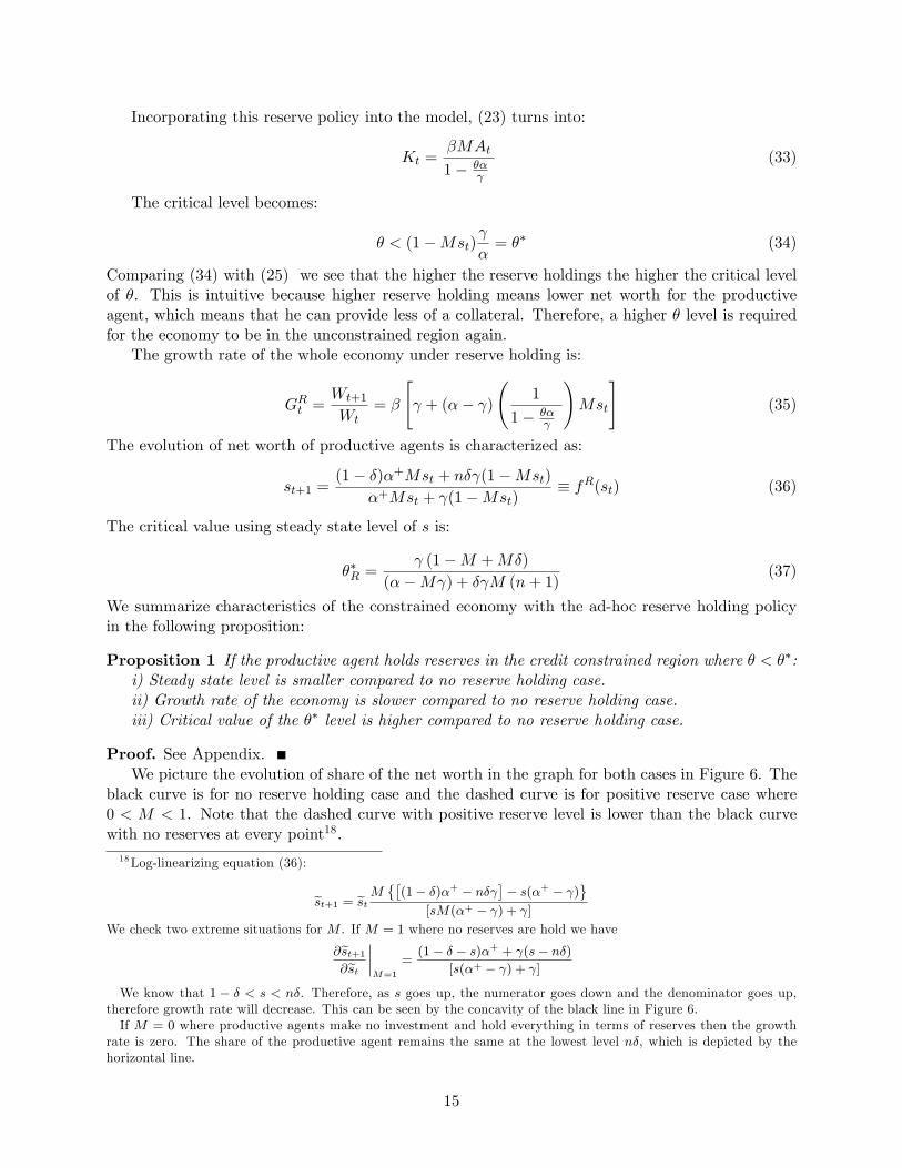
Incorporating this reserve policy into the model, (23) turns into:
Kt =�MAt
1� ��
(33)
The critical level becomes:
� < (1�Mst)
�= �� (34)
Comparing (34) with (25) we see that the higher the reserve holdings the higher the critical levelof �. This is intuitive because higher reserve holding means lower net worth for the productiveagent, which means that he can provide less of a collateral. Therefore, a higher � level is requiredfor the economy to be in the unconstrained region again.
The growth rate of the whole economy under reserve holding is:
GRt =Wt+1
Wt= �
" + (�� )
1
1� ��
!Mst
#(35)
The evolution of net worth of productive agents is characterized as:
st+1 =(1� �)�+Mst + n� (1�Mst)
�+Mst + (1�Mst)� fR(st) (36)
The critical value using steady state level of s is:
��R = (1�M +M�)
(��M ) + � M (n+ 1)(37)
We summarize characteristics of the constrained economy with the ad-hoc reserve holding policyin the following proposition:
Proposition 1 If the productive agent holds reserves in the credit constrained region where � < ��:i) Steady state level is smaller compared to no reserve holding case.ii) Growth rate of the economy is slower compared to no reserve holding case.iii) Critical value of the �� level is higher compared to no reserve holding case.
Proof. See Appendix.We picture the evolution of share of the net worth in the graph for both cases in Figure 6. The
black curve is for no reserve holding case and the dashed curve is for positive reserve case where0 < M < 1. Note that the dashed curve with positive reserve level is lower than the black curvewith no reserves at every point18.18Log-linearizing equation (36):
est+1 = estM ��(1� �)�+ � n�
�� s(�+ � )
[sM(�+ � ) + ]
We check two extreme situations for M . If M = 1 where no reserves are hold we have
@est+1@est
����M=1
=(1� � � s)�+ + (s� n�)
[s(�+ � ) + ]
We know that 1 � � < s < n�. Therefore, as s goes up, the numerator goes down and the denominator goes up,therefore growth rate will decrease. This can be seen by the concavity of the black line in Figure 6.If M = 0 where productive agents make no investment and hold everything in terms of reserves then the growth
rate is zero. The share of the productive agent remains the same at the lowest level n�, which is depicted by thehorizontal line.
15
Proposition 1 explains the impact of reserve holding in a credit constrained economy where thedegree of constraints is determined endogenously. There are three e¤ects which reinforce each other,as a result of leverage e¤ect of the debt. First, as a result of transfer of funds from productive tounproductive agents, the steady state level of the share of productive ones net worth in the economyis smaller and its growth rate is lower compared to no reserves case. Second, as a result of lowerleverage, productive agents can provide less collateral and therefore the critical level of �, wherethey are not credit constrained anymore, goes up. This is important because in an economy wherethere are productive agents and unproductive agents, we expect resources to go to productiveones, so the share of productive ones grow and at some point in future, the share of productiveones are high enough that they are not credit constrained anymore. However, a positive reservepolicy delays this process. Third, the growth rate of the whole economy is lower.
In the next section we see dynamics of the system more clearly.
3 Dynamics
To analyze aggregate dynamics, we calibrate the dynamic system consisting of aggregatedchoice variables fCt; Kt; C 0t; K 0
tgand state variables�Kt�1; K 0
t�1where19:
eCt = �ck eKt�1 + �ck0 eK 0t�1t (38)
eC 0t = �c0k eKt�1 + �c0k0 eK 0t�1t (39)eKt = �kk eKt�1 + �kk0 eK 0t�1t (40)eK 0
t = �k0keKt�1 + �k0k0 eK 0
t�1 (41)
The parameters we use in calibration is given in Table 1 and selected as follows: The productivityrate of the productive agents, �, is taken as 1:06 which equals one plus the average GDP growthrate for 2007 for �ve selected developing countries: Argentina, Chile, Brazil, Korea and Turkey(see Table 2). The productivity rate of the unproductive agents, , is taken as 1:03, which equalsone plus the GDP growth of high income countries de�ned under World Bank classi�cation. Thediscount rate, �, is 0:97 which equals 1= . The � parameter for Markov-switching assumption andthe initial ratio of the population of the productive to unproductive agents, n, are 0:45 and 0:35,respectively. These two numbers are chosen such that � + n� = 0:61 < 1, so the �rst assumptionholds20. Accordingly, to ensure a steady state we chose � = 0:74. Then, �� = 0:75 by (25) so � <�� and we are in the region where both productive and unproductive agents invests. This makes�� = 0:78 < , so the second assumption also holds.
We compare impulse responses to a positive productivity shock on the aggregate levels of con-sumption, capital and wealth for three di¤erent reserve holding ratios. As a benchmark, we assume
19We have used Harald Uhlig�s toolkit and the companion paper Uhlig (1999) both of which can be obtained fromhis website at http://www2.wiwi.hu-berlin.de/institute/wpol/html/toolkit.htm.20Remember that we need this assumption to guarantee a steady state where the capital �ow from the unproductive
agents to the productive ones are sustained in steady state. However, results of the impulse response analysis arevery sensitive to the selection of these two parameters.
16
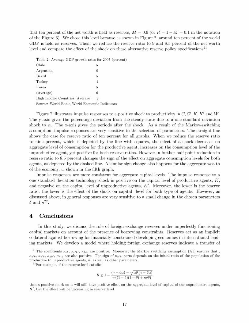
that ten percent of the net worth is held as reserves, M = 0:9 (or R = 1�M = 0:1 in the notationof the Figure 6). We chose this level because as shown in Figure 2, around ten percent of the worldGDP is held as reserves. Then, we reduce the reserve ratio to 9 and 8:5 percent of the net worthlevel and compare the e¤ect of the shock on these alternative reserve policy speci�cations21.
Table 2: Average GDP growth rates for 2007 (percent)
Chile 5
Argentina 9
Brazil 5
Turkey 4
Korea 5
(Average) 6
High Income Countries (Average) 3
Source: World Bank, World Economic Indicators
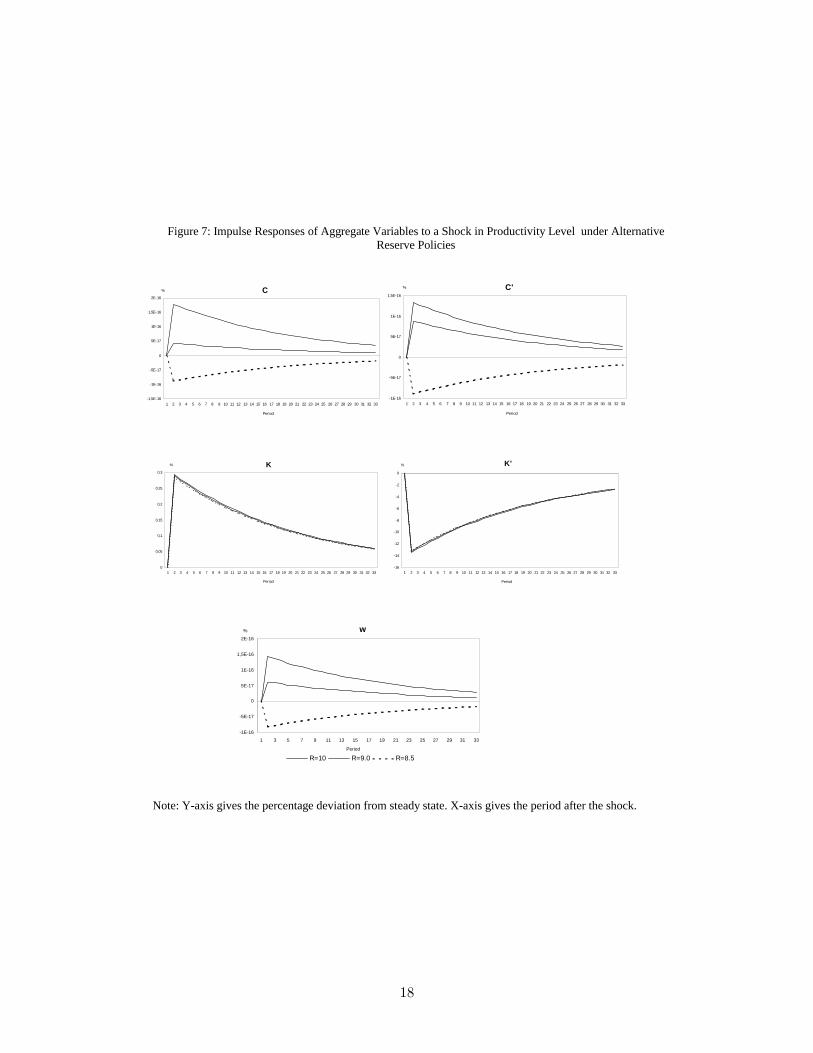
Figure 7 illustrates impulse responses to a positive shock to productivity in C;C 0;K;K 0 andW .The y-axis gives the percentage deviation from the steady state due to a one standard deviationshock to �. The x-axis gives the periods after the shock. As a result of the Markov-switchingassumption, impulse responses are very sensitive to the selection of parameters. The straight lineshows the case for reserve ratio of ten percent for all graphs. When we reduce the reserve ratioto nine percent, which is depicted by the line with squares, the e¤ect of a shock decreases onaggregate level of consumption for the productive agent, increases on the consumption level of theunproductive agent, yet positive for both reserve ratios. However, a further half point reduction inreserve ratio to 8.5 percent changes the sign of the e¤ect on aggregate consumption levels for bothagents, as depicted by the dashed line. A similar sign change also happens for the aggregate wealthof the economy, w shown in the �fth graph.
Impulse responses are more consistent for aggregate capital levels. The impulse response to aone standard deviation technology shock is positive on the capital level of productive agents, K,and negative on the capital level of unproductive agents, K 0. Moreover, the lower is the reserveratio, the lower is the e¤ect of the shock on capital level for both type of agents. However, asdiscussed above, in general responses are very sensitive to a small change in the chosen parameters� and n22.
4 Conclusions
In this study, we discuss the role of foreign exchange reserves under imperfectly functioningcapital markets on account of the presence of borrowing constraints. Reserves act as an implicitcollateral against borrowing for �nancially constrained developing economies in international lend-ing markets. We develop a model where holding foreign exchange reserves indicate a transfer of
21The coe¢ cients �ck, �c0k0 , �kk, are positive. Moreover, the Markov switching assumption (A1) ensures that ,�c0k, �c0k, �kk0 , �k0k are also positive. The sign of �k0k0 term depends on the initial ratio of the population of theproductive to unproductive agents, n, as well as other parameters.22For example, if the reserve level satis�es
R � 1� ( � ��)�p�� ( � ��)
((1� �)(1� �) + n��)
then a positive shock on � will still have positive e¤ect on the aggregate level of capital of the unproductive agents,K0, but the e¤ect will be decreasing in reserve level.
17
Figure 7: Impulse Responses of Aggregate Variables to a Shock in Productivity Level under AlternativeReserve Policies
Note: Yaxis gives the percentage deviation from steady state. Xaxis gives the period after the shock.
resources from productive to unproductive areas, which con�rms the Lucas paradox. We assumea reserve accumulation policy and examined e¤ects of this policy on aggregate macroeconomicvariables in the world economy.
We �rst show that reserve holding lowers the growth rate in global terms, since reserves aretransferred resources from productive areas to unproductive ones. Second, we show that the reserveholding policy have di¤erent impacts in a borrowing constrained economy than an unconstrainedone. In our economy the level of capital market imperfection (degree of credit constraints) isdetermined endogenously by two factors: the level of the productive country�s share in the worldand the di¤erence in productivity level of countries. We compare the evolution of the share ofproductive agents under credit constraints, with and without the reserve policy. As a result ofleverage, reserve holding both lowers the pace of increase in share of productive agents in theeconomy and increases the critical level of �. This is important because in an economy where thereare productive agents and unproductive agents, we expect resources to go to productive ones, sothe share of productive ones grow and at some point in future, the share of productive ones are highenough that they are not credit constrained anymore. However, a positive reserve policy delaysthis process.
Our results contribute to an existing literature that describes the suboptimality of reserveaccumulation process in developing countries. Caballero and Panageas (2008) agree that reserveaccumulation is costly for developing countries that are already constrained �nancially. Theyrecommend use of contingent hedging instruments that would insulate the developing countriesfrom sharp capital reversals. Mendoza et al. (2007) and Durdu et.al (2008) argues that �nancialglobalization is the main determinant of the surge in reserve holdings rather than a motivation tosmooth consumption against cyclical volatility since the latter is not supported by empirics.
We exempted from exchange rate uncertainty in our framework, which could be of interest forfurther studies. Exchange rate level a¤ects the value of reserves and is taken into account undera portfolio management framework. Moreover, while a signi�cant number of developing countrieschose more �exibility in exchange rate o¢ cially, many of them engage in managed �oating toavoid volatility in exchange rates. Central banks require reserves for announced or unannouncedinterventions for this purpose as well. These could be taken as a separate determinant of foreignexchange reserve demand of the developing countries from precautionary savings against suddencapital reversals.
19
References
[1] Aiyagari, S. R., (1994), �Uninsured Idiosyncratic Risk and Aggregate Saving�, Quarterly Jour-nal of Economics, 109, 659-684.
[2] Aizenman, J. and N. P. Marion, (2003), �International Reserve Holdings with Sovereign Riskand Costly Tax Collection�, Economic Journal, 114 , 569�591.
[3] Aizenman, J., Y. Lee, and Y. Rhee, (2005), "International Reserves Management and CapitalMobility in a Volatile World: Policy Considerations and a Case Study of Korea", Journal ofthe Japanese and International Economies, 21(1), 1-15.
[4] Aizenman, J., and Y. Lee, (2007), "International Reserves: Precautionary versus MercantilistViews, Theory and Evidence", Open Economies Review, 18, 191-214.
[5] Alfaro, L., S.K.Özcan and V. Volosovych, (2005), �Capital �ows in a Globilized World: TheRole of Policies and Institutions", NBER Working Paper, No.11696.
[6] Arellano, C and E.G. Mendoza, (2002), "Credit Frictions and Sudden Stops in Small OpenEconomies: An Equilibrium Business Cycle Framework for Emerging Market Crises", NBERWorking Paper, No.8880.
[7] Bar-Ilan, A., N.P. Marion, and D. Perry, (2007), "Drift Control of International Reserves",Journal of Economic Dynamics and Control, 319, 3110-3137.
[8] Bernarke, B.S., (2005), "The Global Saving Glut and the U.S. Current Account De�cit",Remarks At the Sandridge Lecture, Virginia Association of Economics, Richmond, Virginia.
[9] Caballero, R.J. and S. Panageas, (2008), "Hedging Sudden Stops and Precautionary Contrac-tions", Journal of Development Economics, 85, 28�57.
[10] Caballero, R.J. and A. Krishnamurthy, (2001), "International and Domestic Collateral Con-straints in a Model of Emerging Market Crises", Journal of Monetary Economics, 48(3), 513-548.
[11] Calvo, G.A.and C. M. Reinhart, (2002), "Fear Of Floating," Quarterly Journal of Economics,107, 379-408.
[12] Calvo, G., A. Izquierdo and L.F. Mejía, (2004), "On the Empirics of Sudden Stops: TheRelevance of Balance-Sheet E¤ects", NBER Working Paper, No. 10520.
[13] Calvo, G. and E. Talvi, (2006), "The Resolution of Global Imbalances: Soft Landing in theNorth, Sudden Stop in Emerging Markets?", Journal of Policy Modeling, 28, 605�613.
[14] Carroll, C.D., (2001), �A Theory of the Consumption Function, With and Without LiquidityConstraints�, Journal of Economic Perspectives, 15(3), 23-45.
[15] Carroll, C.D. and M.S. Kimball, (2001), �Liquidity Constraints and Precautionary Saving�,NBER Working Paper, No. 8496.
[16] Deaton, A. S. (1991), �Saving and Liquidity Constraints�, Econometrica, 59, 1221�1248.
[17] Dooley, M.D. F.Landau and P. Garber, (2004), "An Essay on the Revived Bretton WoodsSystem", NBER Working Paper, No. 9971.
20
[18] Durdu, C.B., E.G. Mendoza and M.E. Terrones, (2008), "Precautionary Demand for ForeignAssets in Sudden Stop Economies: An Assessment of the New Mercantilism", Journal ofDevelopment Economics, forthcoming.
[19] Feldstein, M., (1999), �A Self-Help Guide for Emerging Markets�, Foreign A¤airs, March/AprilIssue.
[20] Fisher, I., (1933), �The Debt-De�ation Theory of Great Depressions,�Econometrica 1, 337-57.
[21] Flood, R. and N.P. Marion, (2002), �Holding International Reserves in an Era of High CapitalMobility,� in Collins S. M. and D. Rodrik (eds.), Brookings Trade Forum 2001, Washington,D.C.: Brookings Institution Press, 1-68.
[22] Frenkel, J. A. and B. Jovanovic, (1981), �Optimal international reserves: a stochastic frame-work�, Economic Journal, 91, 507-514.
[23] Gertler, M. and K. Rogo¤, (1990), �North-South Lending and Endogenous Domestic CapitalMarket Ine¢ ciencies�, Journal of Monetary Economics, 26, 245�266.
[24] Greenspan, A., (1999), "Currency Reserves and Debt", Remarks to the World Bank Conferenceon Recent Trends in Reserve Management, Washington, DC, 29 April 1999.
[25] Guidotti, P., (1999), Remarks at a G3 Seminar at Bonn, unpublished transcript, April.
[26] Jeanne, O. and R. Ranciere, (2006), �The Optimal Level of International Reserves for EmergingMarket Economies: Formulas and Applications,�IMF Working Paper, 6/229.
[27] Kehoe, P. and F. Perri, (2002), "International Business Cycles with Endogenously IncompleteMarkets", Econometrica 70(3), 907-928.
[28] Kiyotaki, N., (1998), "Credit and Business Cycles", The Japanese Economic Review, 49(1),18-35.
[29] Leland, H. E., (1968), �Saving and Uncertainty: The Precautionary Demand for Saving�,Quarterly Journal of Economics, 82(4), 465-473.
[30] Levy-Yeyati, E., (2008), "The cost of reserves", Economics Letters, 100, 39-42.
[31] Lucas, R., (1990), �Why Doesn�t Capital Flow from Rich to Poor Countries?�, AmericanEconomic Review, 80, 92�96.
[32] Mendoza, E.G., (2006), "Endogenous Sudden Stops in a Business Cycle Model with CollateralConstraints: A Fisherian De�ation of Tobin�s Q", NBER Working Paper, No. 12564.
[33] Mendoza, E. G., V. Quadrini, V.R. Rull, (2007), "Financial Integration, Financial Deepnessand Global Imbalances", NBER Working Paper, No. 12909.
[34] Mishkin F.S., (2007), Systemic Risk and the International Lender of Last Resort, Speechat the Tenth Annual International Banking Conference, Federal Reserve Bank of Chicago,Illinois,September 28, 2007.
[35] Reinhart, C. and K. Rogo¤, (2004), �Serial Default and the �Paradox�of Rich to Poor CapitalFlows�, American Economic Review Papers and Proceedings, 94, 52�58.
21
[36] Rodrik, D., (2006), �The Social Cost of Foreign Exchange Reserves�, NBER Working Paper,No. 11952.
[37] Sandmo, A., (1970), �The E¤ect of Uncertainty on Saving Decisions�, Review of EconomicStudies, 37, 353-360.
[38] Smaghi, L. B., (2006), Conference on Financial Globalization and Integration, Frankfurt amMain, 17-18 July 2006, http://www.ecb.int/press/key/date/2006/html/sp060718_1.en.html.
[39] Taylor, A., (2006), Globalisation: A Historical Perspective,Economics Conference 2006 by Oesterreichische Nationalbank,http://www.oenb.at/en/img/vowitag_2006_09_taylor_tcm16-46347.pdf.
[40] Uhlig, H., (1999), A Toolkit for Analysing Nonlinear Dynamic Stochastic Models Easily, inRamon Marimon and Andrew Scott (eds). Computational Methods for the Study of DynamicEconomies, Oxford University Press, 30-61.
[41] Xu, X., (1995), �Precautionary Saving Under Liquidity Constraints: A Decomposition�, In-ternational Economic Review, 36, 675-690.
22
5 Appendix
Proof of Proposition 1i) It is enough to show that the identity in equation (36) is smaller than the one in (21).
Simplifying we get:st �
+ (1�M) (� + n� � 1) < 0
This always holds since by Assumption 1 we have � + n� < 1 and 0 < M < 1:ii) Since 0 < M < 1 we have GRt > G
ct by comparing (35) and (29)
iii)We want to show that the level of ��R in equation (37) is greater than �� level in equation(31).