MASTER COPY " KEEP THIS COPY FOR REPRODUCTION PURPOSES

Form Approved

AD-A244 711 ATION PAGE I OMB No. 07040 188pvra eI oapr fesione. including the tiefrreviewing Iistruction, searching existingdaasuc.

ng the collecton of Informaton. send comments regarding thi burden estimate or ary other aspect of thito Washington Headquarters Services, Oirectorate for information Operations and keponrs. 12 15 jefferson

of Management and Budget. Paperioric Reduction Project (0704-0183). Washington. OC 20503.

)ATE I3. REPORT TYPE AND DATES COVEREDI 7 Reprint

4. TITLE AND SUBTITLE S. FUNDING NUMBERS L. -

Title show on Reprint 9 .0 3-?'-k'- O :,

6. AUTHOR(S)

Author(s) listed on Reprint

7. PERFORMING ORGANIZATION NAME(S) AND ADORESS(ES) 8. PERFORMING ORGANIZATIONREPORT NUMBER

9. SPONSORING/ MONITORING AGENCY NAME(S) AND ADORESS(ES) 10. SPONSORING/ MONITORINGAGENCY REPORT NUMBER

U. S. Army Research OfficeP. 0. Box 12211Research Triangle Park, NC 27709-2211 , O . "9.J-p14

11. SUPPLEMENTARY NOTESThe view, opinions and/or findings contained in this report are those of theauthor(s) and should not be construed as an official Department of the Armyposition, policy, or decision, unless so designated by other documentation.

12a. DISTRIBUTION/ AVAILABILITY STATEMENT 12b. DISTRIBUTION CODE

Approved for public release; distribution unlimited.

13. ABSTRACT (Maximum 200 words)

ABSTRACT ON REPRINT LD sc'

JAN221 29

14. SUBJECT TERMS IS. NUMBER OF PAGES

16. PRICE ''OE

17. SECURITY CLASSIFICATION 18. SECURITY CLASSIFICATION 1t. SECURITY CLASSIFICATION 20. LIMITATION OF ABSTRACT

OF REPORT OF THIS PAGE OF ABSTRACT

UNCLASSIFIED UNCLASSIFIED UNCLASSIFIED UL

NSN 7540-01-2EO-SSO0 Standard Form 296 (Rev. 2-89)ft"""~e by Ar t4ed. Z39-1

SAIA A_

AIAA 92-0172Identification of Aerodynamic CoefficientsUsing Computational Neural NetworksD.J. Linse and R.F. StengelDepartment of Mechanical

and Aerospace EngineeringPrinceton UniversityPrinceton, NJ

92-00535

30th Aerospace SciencesMeeting & Exhibit

January 6-9, 1992 / Reno, NVFor permission to copy or republish, contact the Americon Institute of Aeronautics and Astronautics370 L'Enont Promenode, S.W., Washington, D.C. 20024

IDENTIFICATION OF A VRODYNAMIC COEFFICIENTSUSING uOMPUTATIONAL NEURAL NETWORKS

Dennis J. Linse" and Robert F. Stengel t

Department of Mechanical and Aerospace EngineeringPrinceton University, Princeton, NJ 08544

Abstract state and control space. While the partitions span thespace, these global models are, in general, not contin-

Precise, smooth aerodynamic models are required for uous across the partition boundaries, much less differ-implementing adaptive, nonlinear control strategies. entiable.Accurate representations of aerodynamic coefficients Maximum-likelihood estimation (MLE) is the mostcan be generated for the complete flight envelope by commonly used technique for extracting aircraft pa-combining computational neural network models with rameters ro nite data 6. Tt-

an Etimt in- efoe-Nodelng araigmforon-ine rameters from flight-test data 16. 71. The ML E tech-an stomation-Before-Modeling paradigm for on-line nique postulates a parametric model (usually linear,training information. A novel method of incorporating more recently nonlinear) of the aircraft and adjusts thefirst-partial-derivative information is employed to esti- prmtr omnmz h eaielgrtmo h

matetheweihtsin idivdua fedforardneual et- parameters to minimize the negative logarithm of themate the weights in individual feedforward neural net- likelihood that the model output fits a given measure-

works for each aerodynamic coefficient. The method mel t u e Fo ot-et data in m od-ment sequence. For flight-test data. individual mod-

is demonstrated by generating a model of the normal els are fit for each test point generating estimates offorce coefficient of a twin-jet transport aircraft from the aircraft stability and control derivatives and uncer-simulated flight data, and promising results are ob- tainty levels. Since the primary use of the derivatives istained, verification of predicted performance. little more than

fairing is done to generate global models through theIntroduction test points [6]. Iterative minimization procedures are

employed, so on-line estimation is not possible.Modern nonlinear control techniques offer exciting po- Non-smooth aerodynamic models can be coercedtential for aircraft control [1-3]. These techniques re- into smooth models with sufficient post-proces-ing.quire comprehensive aerodynamic models that must but this post-processing may reduce the fidelity ofbe differentiable with respect to the state and control. the model. In [2] extensive tabular aerodynamic dataGiven the continuous state and output equations, were fitted with cubic splines before applying NID con-

k = f(x) + g(x)u (1) trol techniques. Cubic splines ensured continuity andsmoothness across subspace boundaries.

y - h(x) (2) An on-line system identification and nonlinear con-

a Nonlinear-Inverse-Dynamic (NID) control law [21 is trol paradigm that integrates computational neuraldeveloped by repeated differentiation of eq. 2 and sub- networks as an aerodynamic modeler within the EBMstitution of eq. 1 until the control appears in each el- framework was presented in [8,9]. Using the plant mea-ement of y or its derivatives. The global represen- surements, z, an extended Kalman-Bucy filter (EKBF)tation of the aerodynamic model contained in f(.), [10] estimates the state of an augmented plant modelg(.), and h(.) must be sufficiently smooth to calcu- consisting of the standard aircraft state, i(t), and thelate such a control law. Many system identification aircraft specific forces and moments, i(t). The neuralmethods used for aircraft fail to provide the globally network learns an aerodynamic model, j(i, u), fromsmooth models needed by these control laws. For ex- *(t), i(t), and the control, u(t). A nonlinear controlample, the Estimation-Before-Modeling (EBM) tech- law using the estimated state, *(t), and the aerody-nique [4, 5] models the aerodynamic coefficients us- namic model, g(x. u), completes the loop and formsing multiple regression schemes on partitions of the an adaptive, nonlinear control system. A block dia-

Graduate Research Assistant, Member AIA. gram of the complete controller is given in Fig. 1.tProfessor, Associate Fellow AIAA. Using the st te/force EKBF and the network esti-

Copyright Q 1992 by the Am-. icar, Institete ur Aeronautics and mation model, excellent matches of aerodynamic coef-Astronautics, Inc. All rights reserved. ficient histories were achieved with a simple neural net-

Presented at the 1992 Aerospace Sciences Meeting,Reno, NV, January 1992. 1

W and b are the weights and biases of the indicated

Nonlinear U Plant zlayers, and cri] is a vector-valued function composedControl Law of individual node activation functions:

9, [. U], o[q] = [a (qj)" .. o,. (q.)] (4)erodynamic 9 State/Force

Aeodel E eBF The outputs of layer k - 1 are connected to the inputs

of layer k successively such that the final form of anNL-layer network is

r(NL) = (N-)(W(NL--)Vr(N'-1)(...

Figure 1: Integration of System Identification and u(W r + b 0 )) + -. )) (5)Nonlinear Control. Defining r = r(° ' as the input vector and z = r(NL) as

the output vector,

work model for single flight conditions, and the corre-sponding functional relationship g(*, u) was well iden-tified [9]. Expanding the ,umber of training flight con- where w is a vector combining all the weights andditions to span the flight envelope continued to yield biases of all the network layers and h(-) is the overallnetwork models with excellent matches of the coeff- function of r and w. A sample two-input/one-output,cient histories; however, g(k, u) and the correspond- one hidden-layer network is given in Fig. 2.ing aircraft stability and control derivatives were notequally well estimated over the entire space.

This paper describes a method of improved aerody- aM 1.]namic modeling that augments the EBM-based iden- W M (2)

tifier and neural network modeler with additional in-formation about the first partial derivatives of the W2 r(2)aerodynamic coefficients. Including both function and r(°)

derivative information in the network training algo-rithm constrains and directs the training by reducingthe number of possible functions that match a par-ticular measurement sequence. Considerable gain is WO) b()_achieved in network accuracy with these methods. andrepresentation of aerodynamic derivatives is improvedsubstantially. Figure 2: A simple feedforward network.

Smoothness of a network function is important if theComputational Neural Networks network is to be used in the suggested nonlinear con-

trol paradigms. The order of differentiability of eq. 6,Computational neural networks are biologically-in- by its construction, is the same as that oi the node ac-spired, massively parallel computational paradigms. tivation functions, a[.). Assuming all activation func-Computational neural networks are used in a variety tions are at least once differentiable, the derivative ofof applications because they are adaptive, they learn the network with respect to its inputs isfrom exampler, and they can provide excellent func-tion approximation. Oh _ )W(.L_1).. 80(F0 )

Multilayer feedforward neural networks combine Or - Oq('L) • -O- t W ° (7)

simple nonlinear computational elements into a lay-ered architecture to compute a static nonlinear func- The derivatives of the activation function vectors aretion. Individual network nodes, with specified non- diagonal matrices: orlinear or activation functions, are grouped together in artdistinct layers, with multiple layers connected for the [(i) ]0

full network. r(k), the output of the kth layer of the Oq(i O 1 (8) 0network, is computed as the nonlinear transformation 0 _"

of the weighted sum of the outputs of the (k - 1)"layer and a bias: The logistic sigmoid is a commonly used node activa-

tion function: 1 ,"r(&) --- ' [W(-)r( - ) + b - ] (3) I(q) = 1 + e-9 (9) "y Codes

and/nr2 " \ t oal

6ONPVCD

74

It is infinitely differentiable, and its first derivative is The extended Kalman filter is a particularly attrac-quite simply calculated as tive alternative method that transforms the optimiza-

tion of eq. 11 and training of eq. 6 into the estimationOa = a(q)[1 - (q)] (10) of a dynamic system [18]. A localized version of the

Oq extended Kalman filter algorithm also has been devel-

A network composed of logistic sigmoid activation oped [19]. Our version of the extended Kalman filter

functions, weights, and biases is infinitely differen- follows the first approach, as described below.tiable. tiable.Extended Kaman Filter for Network Training

Layered feedforward neural networks are closel. re-lated to basis function approximation and regulariza- The state and measurement vectors of a nonlinear,tion theory [11]. In principle, any continuous func- discrete-time system are given bytion (12] or nah-order differentiable function [13] canbe approximated accurately by such networks; how- Xk+i = O(xk) + nk (13)ever, there is no guarantee that the desired network Zk = h(x) + Vk (14)size can be chosen and weights learned from a set of(possibly noisy) training examples. where x, n E R", z, v E R"', and 0(-) and h(.) are gen-

Given a set of 1Vp training examples, {ri, d, , wi,ere eral nonlinear functions in R" and Rm. {nk) and {vk}d. = d(ri) is value of d(.), the function to be approx- are zero mean, white Gaussian processes with covari-imated. for a given input, ri, a suitable least-squares ances Qk and Rk. x0 is a Gaussian random variablecost function is with mean, 10. and covariance, Po.

N, Assuming 0(.) and h(.) are sufficiently smooth, anj = E i (11) extended Kalman filter can be defined for the system,

eq. 13 and 14 (see, e.g., [10,20]). The filter equationswhere the network error vector for the ith trial, e,, is are

c, = d, - h(ri,w) (12) kk- ) = f(*k-l) (15)

P I-) = *I , ] Q I*)After selecting the number of layers and the number p - + Qk (16)

of nodes in each layer, J is minimized with respect to Kk= p(7)I (Hkp(HT + Rk)' (17)w, giving the minimum mean-squared-error network. k

Searching for the weight vector that minimizes eq. 11 xt.= :C + XK {zk - h[* C)1} (18)may be a difficult nonlinear optimization problem.The problem is often constrained by the desire to keep Pk) (I KkHk)P-(I - kHk)T

the weight adjustment algorithm localized, that is, to +KkRkKT (19)update the weights associated with a node only us-ing information available at that node. Localized al- The filter is initialized with io = Ro (the mean) andgorithms simplify hardware implementation although P 0 . The superscript (-) indicates an intermediatethey may ignore coupling information that is impor- value after propagation but before updating with newtant to training, information. Fk and H, are the state and measure-

Traditional nonlinear optimization algorithms in- ment Jacobian matrices:cluding steepest descent, conjugate gradients, and var- 80 (0ious Newton-type algorithms, have been applied to fk = - (20)feedforward computational neural networks [14-17]. ex

Back-propagation, a steepest-descent algorithm, is the Hk = (21)most common algorithm [14]. Modifications and im- oxI,_. (21)provements to the back-propagation algorithm, suchas learning momentum, have been developed [14-16]. A symmetric form is used for the covariance update

Conjugate gradient methods have been successfully (eq. 19) ensuring that Pk remains symmetric and pos-applied to neural networks (see, e.g., [15] for a de- itive definite as long as p(-) is positive-definite and Rkscription of the method). A localized version of the is positive-semidefinite at the expense of more compu-Marquardt-Levenberg lea.t-squares optimization tech- tation [10].nique is developed in [17]. The Marquardt-Levenberg The extended Kalman filter is derived from the lin-algorithr progresses from a steepest-descent alo- ear Kalman filter with the assumption that nonlin-rithm to a quasi-Newton algorithm as optimization ear effects are modeled adequately by the propagationproceeds. Limited testing of the basic Marquardt- of the mean (eq. 15), while disturbances and mea-Levenberg algorithm for a simple network showed no surement errors are small enough to allow linear es-significant benefit in the present application. timates of covariance evolution and measurement up-

3

date (eq. 16-19). The EKF is neither linear nor op- errors in the function value; however, useful trainingtima, but if the system is sufficiently well behaved, information also is contained in the error between de-good results are obtained, sired and actual slopes. If, in addition to the training

data {ri, di}, measurements of the first partial deriva-Modeling the Network for Kalman Filter Train- tives of d(.) evaluated at ri,lng

Identifying the network weight vector w as the state --d (25)Or2 )vector x in eq. 13. a neural network can be expressedOr r,as a nonlinear dynamic system: are available, a new weighted least-squares cost func-

Wk = Wk-1 + nk-I (22) tion can be defined:

zk = h(wk,,rk) + vk (23) I,With the process and measurement noise sequences, J = Z ETR-C, (26){nk) and ftp'}, as defined above, eq. 22 and 23 have (26)

the form of eq. 13 and 14, where O(x) = x and h isdefined by the network forward propagation (eq. 6). where R - 1 is an appropriately dimensioned weightingFor simplicity, the network is assumed to have one matrix. ri is formed by augmenting the original scalaroutput. error, ci, such that

Given a sequence of noise corrupted measurements,{zk}. and the corresponding network input sequence. r d, - h (w.r,) 1{rk). the weight vector, w, is estimated by an ex- = (27)tended Kalman filter. For eq. 22, the state Jacobian Vr_ (r) - - (w.r (,)matrix. Fk. is an identity matrix for all k. This makesthe covariance propagation step, eq. 16. very simple. In eq. 26, R- 1 weights the relative importance of eachComputation of the measurement Jacobian matrix, element of ci, that is. the importance of errors in the

fit of the function, h, compared to errors in the fit ofHk Oh (24) each of the derivatives, Oh/Orj.

OW .wr,) Although any of the previously mentioned networkis a straightforward application of the chain rule, given training algorithms could be reformulated based onthe differentiability of the network nonlinearities and the function-derivative cost. the EKF training methodthe form of eq. 6. Hk has dimension 1 x N,,., where is extended here. The propagation of wk (eq. 22)N,., is the number of weights in the network. remains the same. while the measurement equation

The propagation of wk (eq. 22) is modeled as a dy- (eq. 23) is expanded to include the partial derivatives:namic system driven by a white Gaussian process al-though w is an internal variable that is not subject h (wk.rk) 1to noise. The covariance, Q. of the pseudo-noise se- Zk = ( I +Vk (28)quence, {nk}, controls the convergence of the state I (wkrk)covariance, Pk. In an undriven system (Q = 0). thecovariance matrix converges to zero [21]. This prevents Oh/Or is calculated using eq. 7. With this measure-further state updating since, by eq. 17, Kk is zero if ment equation, the measurement Jacobian matrix be-Pk = O. comes

The order of an extended Kalman filter used as a iiW (29)network training algorithm grows as the length of the H - hnetwork weight vector. The largest network used in LwM JI (w,r,)

this paper is a single hidden-layer network with 9 in- This expanded matrix Hk has dimension (Ni+I)xN.,puts, 20 hidden nodes, and one output, resulting in where pi is the number of network inputs.221 weights and biases. Ordinarily, a Kalman filter of w he N. is the numberofcneworkonputsthis size would be difficult to compute; however, the In the EKF formulation, the covariance, R, of thematrix to be inverted in eq. 17 has dimension m x m, t eas t squenct fuisthe (e as Inwhere m is the output dimension. As m-l, the matrix the weighted least-squares cost function (eq. 26). Itinversion is simply a scalar division. adjusts the relative importance of each of the mea-surements during network training. Equivalently, it

Incorporating Partial Derivatives In Network weights the relative accuracy of each of the measure-

Training ments. While containing more information about thefunction, the partial derivatives may also contain more

For a scalar function d(.), the network training error errors. Thus, a suitable R is important for accurate(eq. 12) is scalar and the cost (eq. 11) is based only on network learning.

4

Training Example Equation 32 represents q variations of +20*/sec atthe given velocity, V. The ift coefficient, C ., isA simple example demonstrates the added benefits of talculaed from e. 30 a i coedith zeroi

function-derivative training (FD-training) over a stan-mean Gaussian noise with a variance of 0.1. Thedard function training (F-training) method. This ex- first network is trained using only function informa-

ample exercises only the aerodynamic model block in tion (F-training). The second network is trained

Fig. 1 using random data rather than the dynamic data with the function-derivative method using additional

that would be produced by simulated or actual flight measurements of 8CL/Oa, mCL/0d, and dCL/ 6

tests. The demonstration function is a lift coefficient (FDtraining). These measurements are also cor-

curve assumed to berupted with zero-mean Gaussian noise with covari-

CL(0,q,6E) = CLsT(O)+ CL,4 + CL, E 6 E (30) ances, 0.5, 6.0 x 10 - 4 , and 0.7. The initial state co-

variance, P 0 , is 104I and the constant process noisew'here a is the angle of attack, = q/2V is the covariance, Q. is 10-3I, where I is the appropriatelynon-dimensionalized pitch rate, and 6 E is the elevator sized identity: matrix. The meaourement noise covan-

deflection angle. Realistic numerical values are cho- ance matrices are identical to the simulated noise used

sen for the aerodynamic derivatives based on a twin- in the example. Thus, for F-training. R -0.1, while

jet transport aircraft [22]. The pitch-rate derivative, for FD-training

CL,(= OCL/N) is 7.0 and the elevator-angle deriva-

tive, CL,, (= OCL/ObE), is 0.006 deg'. The angle- 0.1 0 0 0of-attack contribution, CL,,(a), is a linear function 0 0.5 0 0for low angles of attack and a quadratic function for R 0 0 6.0 x 10- 1 0 (34)

higher angles of attack. It is modeled as 0 0 0 0.7

CL,, (Q) =A comparison of the variation of eq. 30 and its threepartial derivatives to the two network approximations

0.0952a + 0.1048 a < 9C of this function is given in Fig. 4 for angle-of-attack-0.0095- 2 + 0.2667a - 0.6667 a > 90 variations. These plots represent one-dimensional

The restriction of CL to o and 6E inputs is plotted in slices through the fully trained three-dimensional in-Fig. 3. put space. The FD-training is better for the*func-

tion, and it is much better for the derivatives. Therms errors of the function and derivatives for theFD-trained function are all considerably smaller than

Lift Coefficient the F-trained function.The results also indicate the possibility of faster

-" -- learning as measured by the number of training points0.5 . necessary for accurate modeling. The FD-trained net-

0- work quickly learned a representation of the desiredfunction. The total rms error between the function

20 and its three derivatives and the network model ap-proached its minimum value after the presentation of

-5 0 about 500 data points and remained relatively un--- 2 Elevator changed for the remaining points. The F-trained net-

Angle of Atack 20 work required the full 1500 points to reach a level of

accuracy less than that of the FD-trained network.Including partial derivatives in the network training

Figure 3: Example Lift Coefficient, CL, for Fixed 4. process substantially improves the ability of the train-

Using eq. 30 as the desired function, d, two identi- ing process to find an accurate model of the desired

cal feedforward networks with three inputs, one hidden function and its derivatives.

layer of 10 sigmoidal nodes, and one output, are ini-tialized with the same random weights chosen from a Estimating Aerodynamic Coefficientzero-mean Gaussian distribution with variance of 0.1. and Derivative HistoriesThe training data are selected by randomly choosing1500 points from a uniform distribution bounded by The benefits of incorporating gradient information

, [-,5 1901 (31) from the training function into neural network learn-ing are well demonstrated in the previous section. Af-

E [-0.005,0.005] (32) ter a brief summary of the extended Kalman-Buc" fil-6 E E 1-20',20-1 (33) ter equations, the EKBF that estimates the aircraft

1.5

E 0.5 U 0

0~ru Value VluX --- F-Tlraining - - F-Training

- - FD-Training FD-Traning

0 10 20 0 10 20

Angle of Attack, a, degrees Angle of Attack, a, degrees

0.010 20 -

0.08

U% U

0.004 , ,,

0.0

0.002- True Value True Value

F-Training -. F-Training0 - FD-Training - - F1D-Trainins

0 10 20 0 10 20

Angle of Attack, a, degrees Angle of Attack, a, degrees

Figure 4: Network Function and Derivative Comparison at = 0, 6_ = 0.

aerodynamic coefficient histories in addition to state For sufficiently smooth f(.) and h(.), a hybrid ex-histories is described. Subsequently. an extension of tended Kalman-Bucy filter can be defined [101. Thethe state/force EKBF is developed that estimates the hybrid EKBF uses the continuous equations for thedesired partial derivative histories in addition to the state and covariance propagation and the discretecoefficient histories. equations for the gain and measurement update cal-

culations. The continuous equations are

Extended Kalman-Bucy Filter for State and ---= [tk. 11 +Force Estimation th

The state and measurement equations for a combined f[k(r), 0, 7] dr (37)

continuous state/sampled-data measurement system t 'are: P(-)tk] = P[tk-1I + J P(r) dr (38)

k(t) = f [x(t), n(t), t] (35) tj--

Zk = h[x(tk),tk] +vk (36) where

where x E R", z,v E Rm, n E R", and f(.) and h(.) P(C-) = F(r)P(r) + P(r)FT(T) + L(-r)Qc()Lr)

are general nonlinear functions in R" and R'. The (39)

process noise, n(t), is a white, zero-mean Gaussian The gain and update equations (eq. 17-19) are the

random process with spectral density matrix, Qc(t). same as the EKF with the definitions P.-) -The measurement noise sequence, {v&}, is a zero- and :( - ) = V [t]. The inearized matrices F, L,mean, Gaussian random process with covariance, Rk. and H arexO is a Gaussian random variable with mean, jo, and Ofcovariance, Po. F(t) O (40)

6

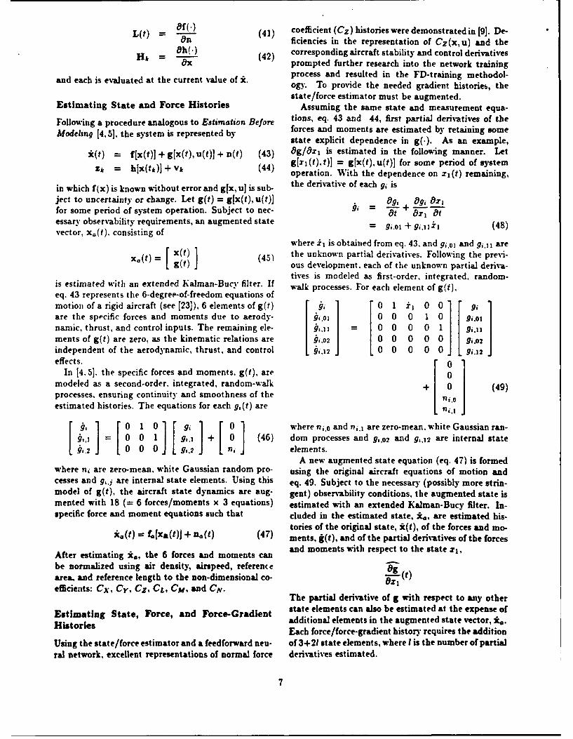
L(t) = Of (41) coefficient (Cz) histories were demonstrated in [9]. De-On ficiencies in the representation of Cz(x, u) and the

Hk = 8h(.) (42 corresponding aircraft stability and control derivativesOx prompted further research into the network training

and each is evaluated at the current value of S. process and resulted in the FD-training methodol-ogy. To provide the needed gradient histories, thestate/force estimator must be augmented.

Estimating State and Force Histories Assuming the same state and measurement equa-Following a procedure analogous to Estimation Before tions, eq. 43 and 44, first partial derivatives of the

Modeling [4, 5], the system is represented by forces and moments are estimated by retaining somestate explicit dependence in g(.). As an example,

x(t) = f[x(t)] + g[x(t),u(t)]+ n(t) (43) Og/Ozi is estimated in the following manner. Let

Zk = h[x(tk)]+ (44) g[xri(t).t)] = gfx(t),u(t)] for some period of systemoperation. With the dependence on zi(t) remaining,

in which f(x) is known ithout error and g[x, u] is sub- the derivative of each g, is

ject to uncertainty or change. Let g(t) = g[x(t), u(t)] _ gD, Ogi OxIfor some period of system operation. Subject to nec- ' I ofessary observability requirements, an augmented state = 9i. +9iIi (48)vector, x,(t). consisting of

where l is obtained from eq. 43. and gi,3o and g,.31 are

X 0 r x(t) 1 (45) the unknown partial derivatives. Following the previ-Sg(t) J ous development, each of the unknown partial deriva-

tives is modeled as first-order, integrated, random-is estimated with an extended Kalman-Bucy filter. If walk processes. For each element of g(t),eq. 43 represents the 6-degree-of-freedom equations ofmotion of a rigid aircraft (see [23]), 6 elements of g(t) i 0 1 il 00 [ iare the specific forces and moments due to aerody- 9,,01 0 0 0 1 0 9'o1namic, thrust, and control inputs. The remaining ele- ij 1, 0 0 0 0 1 9 inments of g(t) are zero. as the kinematic relations are gi.02 0 0 0 0 0 gi,.02

independent of the aerodynamic, thrust, and control I§0~2 0 0 0 0 0 gi2effects. 0

In [4. 51. the specific forces and moments. g(t), are 0modeled as a second-order. integrated, random-walk + 0 (49)processes. ensuring continuity and smoothness of the I i.0estimated histories. The equations for each gi(t) are ni l J

[ 1 [ 0 1 0 gi 1 r 0 1 where nio and ni.l are zero-mean. white Gaussian ran-,. = 0 0 1 g,.1 + 0 (46) dom processes and gi,02 and gi12 are internal state

g,2 0 0 0 9s,2 ni elements.A new augmented state equation (eq. 47) is formed

where ni are zero-mean, white Gaussian random pro- using the original aircraft equations of motion andcesses and gij are internal state elements. Using this eq. 49. Subject to the necessary (possibly more strin-model of g(t), the aircraft state dynamics are aug- gent) observability conditions, the augmented state ismented with 18 (= 6 forces/moments x 3 equations) estimated with an extended Kalman-Bucy filter. In-specific force and moment equations such that cluded in the estimated state, *., are estimated his-

tories of the original state, *(t), of the forces and mo-x.(t) = ffjxa(t)] + ha(t) (47) ments, i(t), and of the partial derivatives of the forces

and moments with respect to the state zl,After estimating i., the 6 forces and moments can

be normalized using air density, airspeed, referene 8garea, and reference length to the non-dimensional co- OX (efficients: Cx, Cy, Cz, CL, CM, and CN.

The partial derivative of g with respect to any other

Estimating State, Force, and Force-Gradient state elements can also be estimated at the expense of

Histories additional elements in the augmented state vector, x.Each force/force-gradient history requires the addition

Using the state/force estimator and a feedforward neu- of 3+21 state elements, where I is the number of partialral network, excellent representations of normal force derivatives estimated.

7

ing envelope, and the remaining three points are dis-tributed through the interior. The dynamic data are

40000 3m w4 * produced using the nonlinear aircraft simulation andDynamic - o .the state/force EKBF. At each point, the aircraft is ex-

30000 .9 ... . .. cited by a specific input, measurements are recorded,and an EKBF is used to estimate the aircraft states

2 5 and forces needed for network training.20000 . 8 ..... To ensure the observability required by the Kalman-

0 *... ... 0 0 Bucy filter, an extensive, but feasible [5], measurementvector is defined. The 13 measured variables are lin-

10000 o7.€ 0 0 v 0 e ear accelerations (a., a., a.), angular accelerationsa a a 0 0 0 (al, am, a.), angular rates (p, q. r), total velocity ('),

0 -. 6 . angle of attack (a), angle of sideslip (10), and altitude0 0.2 0.4 0.6 0.8 1 (h). Process and measurement noise are modeled asMach Number zero-mean, Gaussian random sequences with covari-

ances determined from [5].Starting from a specified trim condition, the aircraft

Figure 5: Twin-Jet Transport Flight Envelope and is excited using a -10 "3211" elevator input. "3211"Training Trim Points. inputs consist of alternating steps of 3. 2. 1, and 1

time-unit widths. With appropriately chosen widths,

Aerodynamic Model Identification from this input history provides a sufficiently rich input forData good estimation of aircraft parameters [24]. Twenty-

second-long measurement histories capturing all of the

The aerodynamic coefficient identification scheme is relevant motion are stored for each dynamic training

demonstrated by generating a model of the normal point.force coefficient. Cz(x. u), of a twin-jet transport air- Using the state/force EKBF. the aircraft state andcraft based on simulated flight-test data. This demon-stration exercises the plant. the state/force EKBF, and ment histories. Initial state, procesf noise, and mea-

the aerodynamic model (in the form of a neural net- surement noise covariance matricef, are based on [5].From the estimated force histories the estimated nor-

work) of Fig. 1. The results of training two identi- mal force coefficient history, Cz(t). is calculated fromcally initialized networks with the EKF F-training and the estimated density. airspeed. and the aircraft wingFD-training methods are presented and compared. A the te ens iting, the rcraft es-single estimated derivative history, Cz. (t), is included area. At the time of writing, the force-gradient es-metod.timation algorithm had not been implemented. Toin the FD-training method. demonstrate the anticipated benefits of the function-

derivative training algorithm. Cz.(t) is calculatedSimulated Flight-Test and Training Data Gen- from the tabulated aerodynamic data using a finite-eration difference scheme and the currently estimated state,

Simulated flight-test data are generated from a full, x(t).

nonlinear, 6-degree-of-freedom model of a twin-jettransport. Standard rigid-body aircraft equations of Neural Network Model and Training Procedure

motion are used 123]. The simulation contains an in- A 9-input, single-hidden-layer network structure withternal aerodynamic model based on extensive tabular 20 logistic sigmoid nodes in the hidden layer and a sin-data and algebraic constraints 122]. Five control inputs gle linear node in the output layer is chosen. The 9drive the system: throttle position (6 T), elevator de- elements of the input vector are Mach number, angleflection (6 _), aileron deflection (6), rudder deflection of attack, pitch rate, density. angle of attack rate, al-( 6 R), and flap position ( 6 r). titude, throttle position, elevator deflection, and Iap

The -ttic training data are generated at 60 trim position:points that span the aircraft operational flight en-velope (Fig. 5). Static training data consist of the Cz = Cz(M,aq,p,d,h,6T,6E,6r) (50)aircraft state and all of the require aerodynamic co-efficients and derivatives for the trimmed condition. This 9-20-1 network has 221 adjustable weights andStatic data points were calculated exactly, as no esti- biases. The network is initialized with random weightsmation was reqidred. selected from a zero-mean, Gaussian distribution with

Dynamic training data are generated around 9 ad- a variance of 0.1.ditional trim points. These points are numbered in The initial state and process noise coiariance matri-Fig. 5. The first six points outline the basic operat- ces for the two training algorithms are identical. The

8

initial state covariance, Po, is 10'1, and the process Coefficient and Derivative Identificationnoise covariance matrix, Q. is 10-21. The large initialstate covariance indicates that the initial weights are Using the procedure outlined above and an FD-unknown. The small process noise covariance allows learning algorithm, a second network is developed tothe weights to converge but prevents the state covari- model Cz(x. u). In addition to Cz(t), a single par-ance from converging to zero. tial derivative history, Cz (t), is used during training.

Training of the networks proceeds in an identical The process noise covariance matrix is

manner for each of the algorithms:

1. Iterate 50 tLies through each of the 60 static R = 1 0o] (51)training points to initialize the network in the 0

neighborhood of the desired function. The larger R(2, 2) element means that the derivative2. Present the first dynamic training history. history is assumed to be noisier and less reliable for

training. As this element gets larger, the results ap-3. Present the 60 static training points. proach that of the F-trained network, and the deriva-

tive information is ignored. Cz(t) and Cz(o) plots for4. Repeat steps 2 and 3 for the nex. dynamic train- the fully trained network at dynamic training point #9

ing point, are given in Figs. 8 and 9. Th' Cz(t) history is not

5. Repeat steps 2 to 4 until the desired convergence as well matched for the FD-trained network as it wasis achieved, for the F-trained network. The Cz(o) match is much

better. The additional training information forces anFor the results presented below, 12 iterations through excellent match of the slope in the training regionsthe 9 dynamic training points were conducted. Since arour A the initial trim condition of 5 angle of attack.each history is 20 sec long. a total of 2160 sec (36 min) The Cz(a) fit deteriorates in the region above approx-of simulated flight data (sampled at 0.1-sec intervals) imately 10'. where the training set contained littleplus 9480 static training points were presented to each data. This mismatch gives rise to the mismatched his-network. tories around 5 and 8 seconds in Fig. 8, where the

angle of attack is outside of the range (-5*, 100). Ad-Coefficient Identification ditional training data in the higher angle-of-attack re-

Using the procedure described above, a neural network gions should make the fit better in those regions.

model of Cz(xu) is developed with the F-trainingmethod. The vrocess noise matrix. R. is 0.1 for thisscalar example. After training, the network model pre-

cisely matches the coefficient histories at each of thedynamic training points. The actual and network es- While present results are promising, the neural net-

timated Cz histories are given in Fig. 6 for dynamic work aerodynamic model was trained and tested in a

training point #9. The histories are indistinguishable, limited setting. Many problems relating to tradition-

The other 8 histories are equally well matched. It ally hard system identification questions remain to be

must be emphasized that these excellent results are addressed before any final iudgments can be made. For

obtained for large maneuvers (angles of attack rang- example, the inputs to the plant must be rich enough

ing from -5 ° to well over the stall angle of attack of for the identifier to extract the best estimate of the

f 16*) at 9 training points covering the entire flight true model from the data. In the examples above,envelope from stall speeds at sea level (Point #1) to the "3211" input provides good excitation of the two

Mach 0.85 at 37,000 feet (Point #4). dominant longitudinal aircraft modes, but it probablyFor use in nonlinear control laws, the network esti- is not rich enough to identify a complete aerodynamic

mate of Cz(x, u) is more important than the estimate model.

of ez(t). The network value of Cz(o) is plotted in It clearly is important not only to span the spaceFig. 7 based on dynamic training point #9. The inter- over which the aerodynamic model is to be defined butsection of the two curves occurs at the trim condition, to minimize correlations in the network input histories.but nowhere else does the model fit well. Although Operating points and maneuvers must be chosen togenerating excellent histories, the network has con- promote orthogonality of the network inputs.verged to an inadequate representation of the under- The state/force/force-derivative EKBF is not yetlying aerodynamic coefficient model. Equally poor re- implemented. Questions relating to observability ofsuits are found at all of the other training points. The the various derivatives are likely to arise. It should benetwork has apparently assigned false dependences of possible to extract the dominant derivatives, such asCz on other network inputs that are closely correlated Cz., with sufficient accuracy to aid the neural networkwith a(t) for the training maneuvers, training process.

9

0.5N Actual Coeffic. tnt - Actual Coefiient

Trained Network - Trained Nework -

00EE

-0.5

LL

-I 2

-1.5 (Two lines effectively identical.) -0 5 10 5 20 "-10 -5 0 5 10 15 20 25 3

Time, t, ec Angle of Attack. a. deg

Figure 6: Normal Force Coefficient History using Figure 7: Normal Force Curve using Function TrainingFunction Training (Mach 0.53, 30,000 ft.). (Mach 0.53, 30.000 ft.).

0.5 .

Actual Coefficient - Actual Coefficient -Trained Network - Trained Network -

0 0

E E

0 5 10 15 20 -10 -5 0 5 10 15 20 2 30Time. t. sec Angle of Anack, a. deg

Figure 8: Normal Forct Coefficient HistorN using Figure 9: Normal Force Curve using Function-Deriva-Function-Derivative Training (Mach 0.53, 30,( ft.). tive Training (Mach 0.53. 30,000 ft.).

Conclusion tained with both static and dynamic inputs in the re-

gions of avilable training data. Dynamic maneuvers

Accurate aerodynamic coefficient models are derived that span the input space and minimize correlations of

from simulated flight-test data using a system iden- the inputs must be defined for effective aerodynamic

tification model composed of an extended Kalman- modeling using computational neural networks.

Bucy filter for state and force estimation and a com-putational neural network for aerodynamic modeling. AcknowledgmentsAn extended Kalman filter network training algorithmbased on function error alone is shown to produce an This research has been sponsored by the FAA andexcellent force-history match, though the functional NA SA Langley Research Center under Grant No. NGLdependence of force on specific inputs is not well iden- 31-001-252 and by the Army Research Office undertified. Including information about derivatives of the Grant No. DAAL03-89-K-0092.function ith respect to its inputs greatly improves thefunctional fit. Networks are wrell-trained using staticinput data uniformly distributed through the input Referencesspace and using dynamic input data generated fromsimulated flight tests. Good functional fits were ob- [1) A. Isidori, Nonlinear Control Systems: An Intro-

10

duction, Springer-Verlag, Berlin, 1989. Propagation," in Parallel Distributed Processing:

[2] S.H. Lane and R.F. Stengel, "Flight Control De- Explorations in the Microstructure of Cognition,sign Using Nonlinear Inverse Dynamics," Auto- D.E. Rumelhart and J.L. McClelland, Eds., MITmatica, Vol. 24, No. 4, Jul., 1988, pp. 471-484. Press, Cambridge, MA, 1986.

[3] G. Meyer, R. Su, and L.R. Hunt, "Application of 15] R. Battiti, "Accelerated Backpropagation Learn-Nonlinear Transformations to Automatic Flight ing: Two Optimization Methods," Complex Sys-Control," Automatica, Vol. 20, No. 1, Jan., 1984, tems, Vol. 3, No. 4, Aug., 1989, pp. 331-342.pp. 103-107. [161 J. Leonard and M.A. Kramer, "Improvement of

[4] H.L. Stalford, "High-Alpha Aerodynamic Mode the Backpropagation Algorithm for Training Neu-Identification of T-2C Aircraft Using the EBM ral Networks," Computers and Chemical Engi-

Method," Journal of Aircraft, Vol. 18, No. 10, neering, Vol. 14, No. 3, Mar., 1990, pp. 337-341.Oct., 1981, pp. 801-809. [17] S. Kollias and D. Anastassiou, "Adapiive Train-

[5] M. Sri-Jayantha and R.F. Stengel, "Drtermina- ing of Multilayer Neural Networks Using a Leasttion of Nonlinear Aerodynamic Coeflicients Using Squares Estimation Technique," IEEE Transac-the Estimation-Before-Modeling Method," Jour- tions on Circuits and Sy-ems, Vol. 36, No. 8,nal of Aircraft. Vol. 25, No. 9, Sep., 1988, pp. Aug., 1989, pp. 1092-1101.796-304. [18] S. Singhal and L. Wu, "Training Feed-forward

[6] K.W. Iliff, "Parameter Estimation for Flight Vehi- Networks with the Extended Kalman Algorithm,"cles." Journal of Guidance. Control, and Dynam- Proceedings of the 1989 International Conferenceics. Vol. 12, No. 5, Sep./Oct., 1989, pp. 609-622. on ASSP, Glasgow, Scotland, May, 1989, pp.

1187-1190.[7] R.V. Jategaonkar and E. Plaetschke, "Identifica-

tion of Moderately Nonlinear Flight Mechanics (19] S. Shah and F. Palmieri, "MEKA - A Fast, Local

Systems with Additive Process and Measurement Algorithm for Training Feedforward Neural Net-Noise." Journal of Guidance, Control, and Dy- works," 1990 International Joint Conference onnamics, Vol. 13, No., 2, Mar./Apr., 1990, pp. 277- Neural Networks, Vol. 3, San Diego, CA, 1990,285. pp. 41-46.

[8] R.F. Stengel and D.J. Linse, "System Identifi- [20] B.D.O. Anderson and J.B. Moore, Optimal Fil-cation for Nonlinear Control Using Neural Net- tering, Prentice-Hall, Inc., Englewood Cliffs, NJ,works," Proceedings of the 1990 Conference on 1979.Information Sciences and Systems, Vol. 2, Prince- [21] F.C. Schweppe, Uncertain Dynamic Systems,ton, NJ, Mar., 1990, pp. 747-752. Prentice-Hall, Inc., Englewood Cliffs, NJ, 1973.

[9] D.J. Linse and R.F. Stengel, "A System Identi- [22] "TCV/User Oriented FORTRAN Program forfication Model for Adaptive Nonlinear Control," the B737 Six DOF Dynamic Model," SP-710-Proceedings of the 1991 American Control Con- 021, Sperry Systems Management, Langley Op-ference, Boston, MA, Jun., 1991, pp. 1752-1757. erations, Hampton, VA, March, 1981.

[10] R.F. Stengel, Stochastic Optimal Control: Theory [23] D. McRuer, I. Ashkenas, and D. Graham, Aircraftand Application, John Wiley & Sons, Inc., New Dynamics and Automatic Control. Princeton Uni-York, 1986. versity Press, Princeton, NJ, 1973.

[11] T. Poggio and F. Girosi, "Regularization Algo- [24] E. Plaetschke, J.A. Mulder, and J.H. Breeman,rithms for Learning That Are Equivalent to Mul- "Flight Test Results of Five Input Signals for Air-tilayer Networks," Science, Vol. 247, No. 4945, craft Parameter Identification," Proceedings of theFeb. 23, 1990, pp. 978-982. Sixth IFA C Symposium on Identification and Sys-

1121 G. Cybenko, "Approximation by Superposition tem Parameter Estimation, Vol. 2, Washington,

of Sigmoidal Functions," Mathematics of Control, DC, June, 1982, pp. 1149-1154.Signals, and Systems, Vol. 2, No. 4, 1989, pp. 303-314.

[13] K. Hornik, M. Stinchcombe, and H. White, "Uni-versal Approximation of an Unknown Mappingand Its Derivatives Using Multilayer FeedforwardNetworks," Neural Networks, Vol. 3, No. 5, 1990,pp. 551-560.

[14] D.E. Rumelhart, G.E. Hinton, and R.J. Williams,"Learning Internal Representations by Error

11