1. Report No. 2. Government Accession No. TX-9411953-1F 4. Title and Subtitle ANALYSIS OF INTERSTATE 35 DESIGN ALTERNATIVES FOR AUSTIN, TEXAS 7. Author(s) Jimmie D. Benson, Timothy J. Lomax, J. Michael Heath, and David L. Schrank 9. Performing Organization Name and Address Texas Transportation Institute The Texas A&M University System College Station, Texas 77843-3135 12. Sponsoring Agency Name and Address Texas Department of Transportation Research and Technology Transfer Office P. O. Box 5080 Austin, Texas 78763-5080 15. Supplementary Notes Technical Report Documentation Page 3. Recipient's Catalog No. 5. Report Date November 1994 6. Perfortning Organization Code 8. Performing Organization Report No. Research Report 1953-1F 10. Work Unit No. (TRAlS) 11. Contract or Grant No. Study No. 7-1953 13. Type of Report and Period Covered Final: September 1990-November 1994 14. Sponsoring Agency Code Research performed in cooperation with the Texas Department of Transportation Research Study Title: Analysis of Interstate 35 Design Alternatives for District 14 16. Abstract The Texas Department of Transportation is considering the upgrade and improvement of Interstate 35 (IH- 35) in the Austin area. Study 7-1953 was directed toward providing assistance to the Austin District to analyze IH-35 design alternatives. TTl assisted the District in reviewing the designs and integrating HOV lanes in the designs. To support the IH-35 analyses, time-of-day travel models were developed and implemented to support peak-period analyses. The Texas Mezzo-Level HOV Carpool Model was also implemented and applied for the IH-35 analyses. Detailed networks were coded and assigned for the various design alternatives. The purpose of this report is to document the model developed, implemented, and applied in the analyses of the IH-35 design alternatives. 17. KeyWords 18. Distribution Statement Travel Forecasting, Peak-Hour Assignments, HOV Carpool Model, Detailed Highway Networks No Restrictions. This document is available to the public through NTIS: National Technical Information Service 5285 Port Royal Road 19. Security Qassif.( of this report) Unclassified Form DOT F 1700.7 (8-72) Springfield, Virginia 22161 20. Security Classif.(ofthis page) Unclassified Reproduction of completed page authorized 21. No. of Pages 90 22. Price
Transcript
1. Report No. 2. Government Accession No.
TX-9411953-1F 4. Title and Subtitle
ANALYSIS OF INTERSTATE 35 DESIGN ALTERNATIVES FOR AUSTIN, TEXAS
7. Author(s)
Jimmie D. Benson, Timothy J. Lomax, J. Michael Heath, and David L. Schrank 9. Performing Organization Name and Address
Texas Transportation Institute The Texas A&M University System College Station, Texas 77843-3135
12. Sponsoring Agency Name and Address
Texas Department of Transportation Research and Technology Transfer Office P. O. Box 5080 Austin, Texas 78763-5080
15. Supplementary Notes
Technical Report Documentation Page
3. Recipient's Catalog No.
5. Report Date
November 1994 6. Perfortning Organization Code
8. Performing Organization Report No.
Research Report 1953-1F
10. Work Unit No. (TRAlS)
11. Contract or Grant No.
Study No. 7-1953
13. Type of Report and Period Covered
Final: September 1990-November 1994
14. Sponsoring Agency Code
Research performed in cooperation with the Texas Department of Transportation Research Study Title: Analysis of Interstate 35 Design Alternatives for District 14
16. Abstract
The Texas Department of Transportation is considering the upgrade and improvement of Interstate 35 (IH-35) in the Austin area. Study 7-1953 was directed toward providing assistance to the Austin District to analyze IH-35 design alternatives. TTl assisted the District in reviewing the designs and integrating HOV lanes in the designs. To support the IH-35 analyses, time-of-day travel models were developed and implemented to support peak-period analyses. The Texas Mezzo-Level HOV Carpool Model was also implemented and applied for the IH-35 analyses. Detailed networks were coded and assigned for the various design alternatives. The purpose of this report is to document the model developed, implemented, and applied in the analyses of the IH-35 design alternatives.
Applications Perspective .................................. 16 Three Model Approach .................................. 16 Texas Auto Occupancy Models ............................. 17 Texas HOV Model Test Results ............................. 18
Time Period % VHT % P-to-A % VHT % P-to-A ======================== ======== ======== ======== ========
Morning Peak Hour 7.03 50.00 5.14 55.00
Afternoon Peak Hour 7.40 50.00 8.11 45.00
Morning Peak 3 Hours 19.04 50.00 14.08 55.00
Afternoon Peak 3 Hours 20.19 50.00 22.92 45.00
Source: "Development of Time of Day Factor Estimates for Truck-Taxi and External Travel Using Survey Data from Other Urban Areas", TTl Technical Memorandum, prepared for the Houston-Galveston Area Council, September 20, 1991 (§).
7
DEVELOPMENT OF HOURLY CAPACITY ESTIMATES
The peak-hour capacity restraint assignments are performed by using the PEAK
CAPACITY RESTRAINT routine in the Texas Large Network Package. To perform these peak
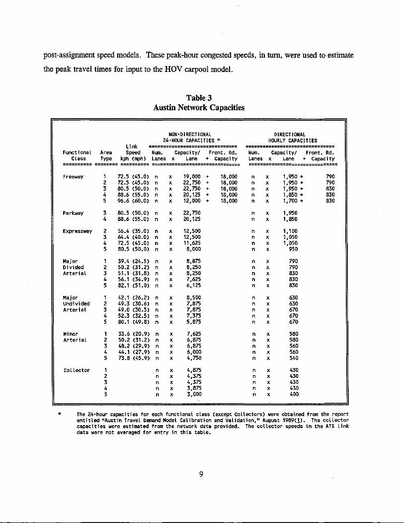
hour assignments, hourly capacity estimates were developed for Austin. Table 3 summarizes the
24-hour network capacities used in the ATS. As may be noted, the capacities were developed to
represent the typical average daily capacity per lane. To remain consistent with this approach,
the hourly capacity estimates were also developed to represent the typical average capacity per
hour per lane.
The hourly capacities developed for use in this study are also summarized in Table 3.
Tables A-I through A-6 (of Appendix A), document the formulas and the typical parameter values
applied in the formulas to estimate the hourly capacities.
Note that the 24-hour capacity data in Table 3 are used to estimate the 24-hour non
directional capacities on links. Hence, the 24-hour frontage road capacities (i.e., the 18,000
vehicles per day) added to the freeway links represent the sum of the capacities of the two frontage
roads (i.e., the frontage road in the A-to-B direction and the frontage road in the B-to-A
direction) .
In contrast, the peak-hour assignments employ a directional network in which the A-to-B
capacity and the B-to-A capacity are estimated separately and entered into different fields in the
link data. The hourly capacity data shown in Table 3 are used to estimate the link capacities by
direction. Hence, the hourly frontage road capacities added to the freeway directional link
capacity represents only the frontage road capacity in one direction. For these frontage road
estimates, two-lane frontage roads were assumed. Further, it was assumed that one of the two
lanes is generally dedicated to the freeway access/egress; and, therefore, only one lane remains
available for through traffic. The typical average capacity per hour per lane for major divided
arterials was used to estimate these frontage road capacities.
These hourly capacities have been used to prepare a 2020 Austin peak-hour network for
use in the HOV carpool modeling efforts. A peak-hour capacity restraint assignment was
performed using this network. The results of the peak-hour assignment were used to apply the
8
post-assignment speed models. These peak-hour congested speeds, in turn, were used to estimate
the peak travel times for input to the HOV carpool model.
Link =============================== =============================== FunctionaL Area Speed Num. Capacity! Front. Rd. NI.IIl. Capacity! Front. Rd.
CLass Type kph (mph) Lanes x Lane + Capacity Lanes x Lane + Capacity ========== ======== ========== =============================== ===============================
Freeway 1 72.5 (45.0) n x 19,000 + 18,000 n x 1,950 + 790 2 72.5 (45.0) n x 22,750 + 18,000 n x 1,950 + 790 3 80.5 (50.0) n x 22,750 + 18,000 n x 1,950 + 830 4 88.6 (55.0) n x 20,125 + 18,000 n x 1,850 + 830 5 96.6 (60.0) n x 12,000 + 18,000 n x 1,700 + 830
Parkway 3 80.5 (50.0) n x 22,750 n x 1,950 4 88.6 (55.0) n x 20,125 n x 1,850
Expressway 2 56.4 (35.0) n x 12,500 n x 1,100 3 64.4 (40.0) n x 12,500 n x 1,050 4 72.5 (45.0) n x 11,625 n x 1,050 5 80.5 (50.0) n x 8,000 n x 950
Major 1 39.4 (24.5) n x 8,875 n x 790 Divided 2 50.2 (31.2) n x 8,250 n x 790 ArteriaL 3 51.1 (31.8) n x 8,250 n x 830
4 56.1 (34.9) n x 7,625 n x 830 5 82.1 (51.0) n x 6,125 n x 830
Major 1 42.1 (26.2) n x 8,500 n x 630 Undivided 2 49.3 (30.6) n x 7,875 n x 630 ArteriaL 3 49.0 (30.5) n x 7,875 n x 670
4 52.3 (32.5) n x 7,375 n x 670 5 80.1 (49.8) n x 5,875 n x 670
Minor 1 33.6 (20.9) n x 7,625 n x 580 ArteriaL 2 50.2 (31.2) n x 6,875 n x 580
3 48.2 (29.9) n x 6,875 n x 560 4 44.1 (27.9) n x 6,000 n x 560 5 73.8 (45.9) n x 4,750 n x 540
CoLLector 1 n x 4,875 n x 430 2 n x 4,375 n x 430 3 n x 4,375 n x 430 4 n x 3,875 n x 430 5 n x 3,000 n x 400
* The 24-hour capacities for each functionaL cLass (except CoLLectors) were obtained from the report entitLed "Austin TraveL Demand ModeL CaLibration and VaLidation," August 1989(1). The coLLector capacities were estimated from the network data provided. The coLLector speeds in the ATS Link data were not averaged for entry in this tabLe.
9
CAPACITY RESTRAINT ASSIGNMENT MODEL
The peak-hour assignment performed under this study used the ASSEMBLE PEAK
NETWORK and PEAK CAPACITY RESTRAINT routines of the Texas Large Network Package.
During the early portion of the study, the Texas capacity restraint procedure was used. The Texas
procedure is an iterative technique which requires user specified iteration weights. The peak-hour
assignments were performed using six iterations with the following iteration weights: 10, 10, 20,
20,20, and 20 percent. In November 1992, an equilibrium assignment option was implemented
in the PEAK CAPACITY RESTRAINT routine by TTl under another study funded by the
TxDOT (2). The equilibrium technique uses an optimization technique to estimate iteration
weights. The equilibrium assignment procedure is currently considered the assignment technique
of choice. Hence, it was adopted for use in this study as soon as it became available.
SPEED ESTIMATION MODELS
The peak-hour speeds are estimated using the results from the peak-hour capacity restraint
assignment. These assignments are used to estimate the directional volume-to-capacity (vIc) ratio
for each link. Since this study is focusing on the IH-35 alternatives, the principal focus will be
the free-flow travel time estimates and the potential time savings offered to carpools by the HOV
facilities being studied.
The speed estimation models employed in the Houston-Galveston region were implemented
and calibrated by TTl under studies sponsored by the H-GAC. These models have been adapted
for application to the Austin peak-hour network. Separate speed models are used for freeways
and for arterial and collector streets. The following describes the two speed estimation models.
Freeway Model
The speed estimation procedures described in a report (prepared by Cambridge Systematics
for the EPA in September 1991) entitled "Highway Vehicle Speed Estimation Procedures For Use
In Emissions Inventories" were selected for implementation and calibration for the Houston
Galveston Region. The validation results using this technique has displayed very favorable
10
results. This freeway speed estimation procedure has therefore been employed in the study of the
IH-35 alternatives under this study.
The freeway speed estimation model relies primarily on the speed estimation techniques
described the Highway Capacity Manual (which will be referred to as the HCM). The extensions
of the models are similar to those used in Phoenix, but the model coefficients were revised during
in the Houston-Galveston Region during the validation process. The methods rely on the
estimated vIc ratio as a key measure of congestion for estimating the congested speed based on
a link's capacity restrained volume.
The basic freeway model focuses on the decay in speed from a free-flow speed to a Level
of-service E (LOS E) speed as the level of congestion on link increases from a zero-volume
condition to a vIc ratio of 1.00. Table 4 lists the speed reduction factors (SRF) currently being
used in the model (Q). In an earlier version of the model, the speed reduction factors were derived
from Figure 3-4 of the HCM (1). The updated speed reduction factors were derived from the
Chapter 3 revisions to the HCM recommended by the Freeway Subcommittee of the Highway
Capacity and Quality of Service Committee of the Transportation Research Board. For vIc values
not included in the Table 4, the speed reduction factors are obtained by interpolating values from
Table 4. For example, the speed reduction factor for a vIc ratio of 0.65 would be obtained by
interpolating between 0.243 and 0.350 (Le., the values for vIc ratios of 0.6 and 0.7 respectively).
After obtaining the speed reduction factor for a freeway link based on its vic ratio from
the capacity restrained assignment results, the link's congested speed is computed as follows:
where:
Sp
SFF
SE
SRF
-
-
-
-
Predicted speed for the link
The free-flow (or zero-volume) speed of the link
The LOS E speed of the link
The speed reduction factor corresponding to the link's vIc ratio.
For the Austin assignments, the freeways are assumed to have a speed limit of 88.5 kph
(55 niph). In the rural areas freeways are assumed to have a 104.6 kph (65 mph) speed limit.
11
The speed limit is used to estimate the link's free-flow speed. Recognizing the tendency of drivers
in Texas to speed (particularly under free-flow conditions) the freeway free-flow speed are
estimated by adding from 3.2 to 12.1 kph (2 to 7.5 mph) to the freeway link's speed limit,
depending on its location. This tendency was clearly reflected in the observed speeds for the
As may be noted, the preceding technique can be used only for volume to capacity ratios
up to 1.0. Because traffic assignments occasionally exceed these limits, a model extension is
needed. In the current version of the model, an extension based on the BPR model (currently used
in the Houston models) was implemented in the Austin model (Q). The model extension for
freeways and expressways with a volume to capacity ratio over 1.0 is:
Sp = SPI * [1.15/(1.0 +(0.15*(V/C)4)]
12
where:
Sp = predicted speed for the link
SPl - the speed estimated on the link for a vIc ratio of 1.0 using the
freeway model
VIC = the capacity restraint directional vIc ratio constrained to a maximum
value of 1.5.
Arterial and Collector Street Model
Since the primary focus of this study is the IH-35 alternatives, a simpler model was
selected for application to the arterial and collector streets. The model selected was the traditional
BPR impedance adjustment model. The BPR model has also been employed in earlier versions
of the Houston model and found to provide good estimates of peak-hour travel times. The results
of the BPR model applications in Houston are described in a report entitled "Development, Update
and Calibration of 1985 Travel Models for the Houston-Galveston Region" (~).
A constrained version of the traditional BPR impedance adjustment function was used the
estimate these peak-hour directional speeds. The BPR function is applied as follows:
where:
Sp
So
VIC
= = =
estimated peak-hour speed based on the directional vic ratio
estimated zero-volume speed
capacity restraint directional vIc ratio constrained to a maximum
value of 1. 5.
Since the network data contain only the 24-hour speeds on arterials and collectors, the zero
volume speeds must be estimated for application of the BPR function. The zero-volume speeds
for the non-freeway facilities were simply estimated by dividing the 24-hour speed by 0.92 and
rounded to the nearest integer speed.
13
PEAK-HOUR TRAVEL TIME ESTIMATES
The peak-hour network used to perform the peak-hour capacity restraint assignment is
coded without the HOV links represented in order to get an estimate of the peak travel times
without HOV facilities. The normal 24-hour speeds are used as input to the capacity restraint
assignment. The post-assignment directional peak-hour speeds (estimated by the speed models
using the capacity restrained peak-hour assignment results) are then inserted into the link data for
the alternative being studied. These speeds represent the best available estimate of the expected
operational peak-hour speeds on the system. The ASSEMBLE PEAK NETWORK and BUILD
TREES routines of the Texas Large Network Package are used to develop the peak-hour zone-to
zone peak-hour travel time estimates using the normal highway facilities (i.e., without the HOV
carpool facilities).
The proposed HOV carpool links are then inserted into the link data containing the
estimated peak-hour speeds. The ASSEMBLE PEAK NETWORK and BUILD TREES routines
are then applied using the HOV network to develop the peak-hour zone-to-zone travel time
estimates for carpools using the HOV facilities. The differences in these travel time estimates
provide the HOV model with an estimate of the potential time savings for HOV carpools.
14
CHAPTER III. HOV CARPOOL MODEL
Historically, the emphasis of highway planning has been to assess the capability of a
proposed system of highway improvements to serve the forecast travel demands. Freeway system
expansion is often necessary to serve the projected demand. However, the planned addition of
more traffic lanes by itself is often not sufficient to provide the capacity needed to prevent severe
peak-period congestion and travel time delays.
In such situations, consideration is often given to providing special lanes designated for
the exclusive use of high -occupancy vehicles (HOVs) such as buses and carpools. Experience has
shown that these special lanes can be an effective means of moving large volumes of persons
during highly congested peak periods. During the peak hour it is estimated that HOV facilities
can move the person trip equivalent of three normal traffic lanes. Obviously, the magnitude of
the person movement capability of HOV lanes can significantly enhance the peak-period person
movement capability of a severely congested freeway corridor. This demonstrated ability of HOV
lanes (transitways) to move high volumes of peak-period commuters in congested freeway
corridors has led to the large commitment to HOV lanes in Texas. Careful consideration is being
given to incorporating exclusive HOV lanes in the proposed 1lI-35 improvements. An important
task of this study was to assess the potential carpool usage for these HOV facilities.
TEXAS MEZZO-LEVEL HOV CARPOOL MODEL
From a travel demand modeling perspective, HOV carpool demand modeling is a new and
evolving area with a relatively limited experience base. In some of the recently developed mode
choice models, an HOV carpool component has been included in the model. However, the mode
choice models for most urban areas do not include an HOV carpool component. The Texas
Mezzo-Level HOV Carpool Model was implemented in the Texas Travel Demand Package by TTl
for TxDOT to provide for the analysis of HOV facilities in such areas (lll). The model is
essentially a post-mode choice model which can be used to estimate the potential homebased work
carpool usage for a proposed HOV facility.
15
Applications Perspective
The model is implemented as the HOVMODEL routine in the Texas Trip Distribution
Package (11). The application of the model requires the following inputs:
• the homebased work (HBW) person trip table for the region
• the morning peak zone-to-zone travel times for normal highway trips
• the morning peak zone-to-zone travel times for carpools eligible to use HOV
facilities
• the sector-to-sector base mode split for HBW trips
• the base auto occupancy estimates for HBW trips
Based on the differences in travel times for normal highway trips versus HOV carpool trips, the
model estimates the change in auto occupancy that can be anticipated due to the implementation
of the proposed HOV carpool facility. Using this information, the model estimates and outputs
two HBW vehicle trip tables:
• the HBW carpool trips expected to use the HOV facility
• the HBW vehicle trips expected to use only the normal highway facilities
The model looks at each zone pair in the region. If the use of the HOV carpool facility
offers more than a minimum travel time savings, then the HBW person trips for that zone pair are
considered "candidate" trips for possible carpooling. The regional model data are used to prove
base information on the transit mode share and auto occupancy assuming that the facility is not
open to carpools. Based on comparison of the peak travel times on normal highway versus the
time for HOV carpool users, the carpool model estimates the shift in auto occupancy expected.
The Texas auto occupancy models are applied to the non-transit candidate trips to estimate the
vehicle trips by integer occupancies (i.e., 1 person, 2 persons, 3 persons and 4 + person vehicles).
The vehicle trips are separated into the two output trip tables.
Three Model Approach
Based on the review of the available HOV lane carpool demand models, a model
developed by Barton Aschman and Associates, Inc. (BAA) for the Atlanta Regional Commission
was selected for "mezzo-level" adaptation in the Texas Package (10). The Atlanta model provided
16
for the analysis of either 3+ or 4+ person carpools. For Texas applications and based on the
Houston experience, TTl modified and extended the models to accommodate a 2 + person carpool
defmition.
One of the very salient features of the Atlanta Model was its use of three models. The
three models, originally developed for use in the Washington, D.C. region, are: (1) the travel time
ratio model developed by JHK & Associates for use in estimating carpools in the Shirley Highway
and IH-66 corridor inside the Beltway; (2) the logit model developed by BAA for use in
estimating carpools in the Bolling/Anacostia Corridor; and (3) the time savings model developed
by the Metropolitan Washington Council of Governments for estimating carpools for long-range
planning. These three models are described in detail in Appendix B of this report.
In their review and analyses of the three models, BAA concluded that it was impossible
to judge with any degree of assurance which of the three models is more accurate for all
conditions and, indeed, for any specific condition. All three models have been accepted and used
for planning HOV facilities in the Washington, D.C. region. Based on their analyses, it was
recommended that an HOV carpool model make use of all three models. Hence, each of the three
models is applied to each zonal interchange to estimate the HOV carpools. A weighted average
of their estimate is computed to the final "best estimate."
The three models do not require information on the characteristics of the trip maker such
as income or automobiles available. This is certainly a salient feature both from a "mezzo-level"
adaptation perspective and from a "portability" perspective.
The three models are used as "shift" models with the region's travel demand model data
used as the basis for the shift. This methodology not only reduces the potential errors in the
models but allows the HOV model's estimates to be compatible with other estimates and forecasts
being made for the area without the use of carpool facilities, another very desirable feature from
a "portability" perspective.
Texas Auto Occupancy Models
A set of average auto occupancy models (which are referred to as the base auto occupancy
models) is needed for a post-mode choice implementation of the HOV model. These auto
17
occupancy models are used to estimate the percentage of vehicles by integer occupancy groups
(Le., 1, 2, 3 and 4+ person autos) for a specified average auto occupancy group. In the Atlanta
version of the model, the base auto occupancy models were developed using data from the
Washington, D.C., area and only allow consideration of average auto occupancies as low as 1.15.
This minimum limit of 1.15 for the specified average auto occupancy for HBW trips was
considered a serious constraint for Texas applications. While 1.15 may be considered as a
relatively low average auto occupancy for HBW trips in the Washington, D.C. area, it is probably
very close to the regional average for the HBW trips in the larger urban areas in Texas. Indeed,
the 1984 travel survey for Houston indicated a regional average auto occupancy of 1.13 for HBW
trips.
A new set of auto occupancy models were, therefore, calibrated which are felt to be more
representative of urban areas of Texas. The new models allow the estimation of integer car
probabilities in cases where average auto occupancy is less than 1.15. The new Texas Base Auto
Occupancy Model, like the Atlanta model, is a set of regression models. The new model was
developed through the use of vehicle classification data from the Houston area. The new model
allows for consideration of average auto occupancies as low as 1.06. Appendix B contains a
detailed description of the new base auto occupancy model.
Texas HOV Model Test Results
The test and evaluation of the Texas Mezzo-Level HOV Carpool Model focused on the
ability of the model to reasonably replicate observed levels of carpool usage on the HOV facilities
in Texas. Two sites were selected for testing the model: (1) the Katy Transitway in Houston and
(2) Phase I of the Gulf Transitway in Houston.
The Katy Transitway, which began operation in 1984, is an 18.5 kIn (11.5 mile) limited
access facility which exists in the median section of the Katy Freeway (IH-I0W) between SH-6
and the West Loop (IH-610). Intermediate access points are provided from a park-and-ride lot
at SH-6 and from the freeway median near Gessner Road. Extensive data exist regarding carpool
operation on the Katy Transitway, as it is one of the most studied facilities of its kind in the
18
country. The availability of these data made it the primary focus for the testing and evaluation
of the Texas model.
The Phase I portion of the Gulf Transitway is a 9.5 Ian (5.9-mile) facility which operates
in the median section of the Gulf Freeway (lli-45S) and runs from just south of the South Loop
(lli-610) to Dowling Street in downtown Houston, with intermediate access points located at the
South Loop and at a transit center. Although it was felt that the Phase I portion of the Gulf
Transitway was a marginal facility in terms of length of operation (relative to the Katy
Transitway), the facility was used as a secondary site for model testing and evaluation. The
primary reason for choosing the Phase I Gulf Transitway as a test site was that it was the only
other operating HOV facility in the state on which carpools were allowed and for which data
existed at the time of the study.
The test results from the two applications of the Texas mezzo-level HOV carpool model
were judged to be "good" (i.e., within + 12.5 percent of observed volumes). Since the models
are applied as "shift" models using the regional model results, it was felt that the model could be
expected to generally produce reasonable carpool estimates which are consistent with the regional
forecast. Based on the test results, it was recommended that the Texas Mezzo-Level HOV
Carpool Model be incorporated in the Texas Trip Distribution Package software for application
in Texas cities. Based on these results, the model has been used in the Houston-Galveston area
for the past four years.
AUSTIN APPLICATIONS
The Texas Mezzo-Level Carpool Model forecast the HOV carpools which would be
expected to use the HOV facilities being considered for implementation in the IH-35
improvements. These analyses were performed under Task 3 of this study. The following briefly
describes the data used as input to the HOV model and briefly summarizes the model results.
Data Inputs and Parameters
The fIrst major input to the HOV model is the forecast HBW person trip table for the
region. The ATS 2020 HBW person trip table (provided to TTl by the City of Austin in May
19
1992) was used in this modeling effort. This 24-hour trip table (in production-to-attraction
format) is the official HBW person travel forecast for the region.
The next key inputs to the HOV model are zone-to-zone peak-hour travel time estimates
based on the forecast travel for the region. The time-of-day models (discussed in Chapter IT) were
applied to estimate the 2020 morning peak-hour volumes and congested speeds. The congested
directional speed estimates were inserted into a peak-hour network for use in estimating the zone
to-zone travel times using only the normal highway facilities. This network is generally referred
to as the "normal highway network." A second peak-hour highway network was then developed
by inserting links to represent the HOV carpool facilities proposed for the IH-35 improvements.
The second network was used to estimate the zone-to-zone peak-hour travel times for trips
eligible to use the HOV carpool facilities. This second network is generally referred to as the
HOV carpool network.
The sector-to-sector HBW mode split estimates for 2020 are also a key input to the HOV
model. The ATS 2020 HBW transit person trip table was also provided to TTl in May 1992 for
use in these analyses. Using the transit trip table and the person trip table, the sector-to-sector
mode shares were computed. The ATS uses a very detailed sector structure consisting of 90
sectors in model applications. The ATS sector structure was used to complete the sector
interchange mode shares for input to the HOV model.
The ATS uses an average auto occupancy of 1.13 for converting non-transit HBW person
trips to vehicle trips. The Austin CBD, the State Capitol Complex, and the University of Texas
at Austin areas (Le. Sectors 64 and 58) are already intensely developed and experience parking
limitations. It is certainly reasonable to expect that the 2020 HBW trips attracted to these areas
will have a somewhat higher auto occupancy than the remainder of the region. A conservative
auto occupancy rate of 1.20 was assumed for HBW trips attracted to these areas in the HOV
analyses. The remainder of the sector interchanges used the ATS regional auto occupancy
estimate of 1.13.
In applying the HOV model, it is desirable to estimate terminal times. The default
production and attraction terminal times were set to 1.0 and 2.0 minutes, respectively, in the HOV
model runs. The default terminal times were used for all areas except the CBD, Capitol Complex,
20
and UT areas (Le., Sectors 64 and 58). For these areas, production and attraction terminal times
of 2.0 and 5.0 minutes, respectively, were used.
The Austin HOV model applications used a carpool defInition of 2 + persons/vehicle (Le.,
carpools with 2 or more persons in the vehicle are allowed to use the HOV carpool facilities).
Only HBW trips which could save 2.5 minutes or more in the peak period were considered
potential candidates for HOV usage.
HOV Results
The final HOV model applications were performed in the fall of 1992. The following
briefly summarized the HOV model results.
The ATS 2020 forecast for the region estimates 1,580,122 HBW person trips for the
region. An estimated 10.44 percent of these trips will use the planned transit system for the
region. The HOV carpool model found that approximately 94,147 of the 1,580,122 HBW person
trips could save 2.5 minutes or more using the proposed lli-35 carpool facilities. Approximately
10,283 HBW carpools would be expected to use the proposed facilities each day. These carpools
would be expected to carry about 22,211 persons representing an average occupancy on the
carpool lane of 2.16 persons/vehicle. Of the 94,147 candidate HBW person trips, 29.6 percent
would be expected to remain on transit and 44,056 (or 46.8 percent) would be expected to travel
in single occupant vehicles. The 22,211 person trips expected to travel by carpool on the HOV
facility represents 23.6 percent of the 94,147 candidate HBW trips. The carpool model indicates
that an estimated additional 3,142 carpools would be formed to take advantage of the HOV
carpool facilities.
It should be noted that the 22,211 HBW person trips expected to travel by carpool on the
HOV facility is by no means all of the person trips expected to use the facility. A significant
portion of the 27,880 candidate HBW person trips traveling by transit will likely be on buses on
the HOV facility. Also, while work trip carpools would generally be expected to account for most
of the carpool trips on the facility, there will be a significant number of carpools on the facility
which are not HBW trips. For example, it is reasonable to expect a significant number of non-
21
work carpools traveling on the HOV facility to the University of Texas. These trips are not
accounted for in the HOV carpool model.
AIR QUALITY ANALYSES
As a part of the regional travel analyses performed under Task 3, an analysis of the mobile
source emissions impacts of the proposed IH-35 improvements was performed. The following
briefly summarizes the results of these analyses.
The No-Build Alternative
To assess the impact of the proposed IH-35 improvements on mobile source emissions, a
no-build alternative was defmed. To create the no-build alternative network, the capacities for
the IH-35 links in the 2020 network were reduced to the current 1993 levels. All other planned
improvements in the 2020 network remained unchanged. Since the no-build alternative will not
have an HOV lane, the original ATS vehicle trip tables developed prior to the application of the
HOV model were used for the assignment. A capacity restraint assignment was performed for
the no-build alternative.
For the build alternative, the assignments developed in the HOV analyses were used. This
allowed the air quality analyses to reflect the impact of both the added HOV lanes and the added
capacity for the normal highway travel.
Emissions Estimation Methodology
The air quality analyses were performed using the Texas Mobile Source Emissions
Software. The Texas Mobile Source Emissions Software is a series of programs developed by the
Texas Transportation Institute to facilitate the estimation of mobile source emissions. The methods
used in applying this software have been successfully used in developing the mobile source
emissions estimates for air quality analyses in the EI Paso, Beaumont-Port Arthur and Victoria
regions. This methodology is also similar the procedures used for the Dallas-Fort Worth mobile
source emissions estimates. Portions of this software are also employed in the Houston-Galveston
.region for their emissions estimates.
22
The following briefly summarize the program and procedures used in developing the
emissions estimates for both the build and no-build alternatives. The three programs in the Texas
Mobile Source Emissions Software for the Austin analyses were:
PREPIN The PREPIN program was developed to facilitate the estimation of time-of
day VMT and speeds for air quality analyses. The program inputs a 24-
hour assigrunent and applies the needed time-of -day factors to estimate the
directional time-of-day travel. The Dallas-Fort Worth speed models are
used to estimate the operational time-of -day speeds by direction on the
links. Special intrazonal links are defmed, and the VMT and speeds for
intrazonal trips are estimated. These VMT and speeds by link are
subsequently input to the IMPSUM program for the application of
MOBILE5a emission factors.
POLFAC5A The POLF AC5A program is used to apply the MOBILE5a program to
obtain the emission FACTORS (rates). The MOBILE5a emission factors
are obtained for eight vehicle types and 63 speeds (Le., 3 mph through 65
mph) for each vehicle type. Hence, there are 504 factors (Le., 8 x 63 =
504) for each pollution type. Three pollution types are computed: VOC,
CO and NOx. Hence, for a given application there are 1512 emission
factors. These emission factors are output to an ASCII file for subsequent
input to the IMPSUM program. The POLFAC5A program is applied for
each time-of-day time period being used. These time-of-day emission
factors are applied using the IMPSUM program to time-of-day VMT
estimates by link.
IMPSUM The IMPSUM program applies the emission rates (obtained from
POLFAC5A) and VMT mixes to the time-of-day VMT and speed estimates
to estimate the emissions. The basic input to IMPSUM include:
1. VMT mix by county and roadway type.
2. MOBILE5a emission factors developed using
POLFAC5A by county.
23
3. Abbreviated assignment results by link input for the subject time
period. The PREPIN program allows the user to estimate the VMT
and speed on each link by time period. For each link, the following
infonnation is input to IMPSUM: roadway type number, VMT on
link, operational speed estimate, and the link distance.
Using these input data, the VMT for each link is stratified by the eight
vehicle types, and the MOBILES a emissions factors are applied to estimate
the mobile source emissions for that link.
The PREPIN software was applied to both the build and the no-build alternatives to produce the
time-of-day VMT and speed estimates for each alternative. The four time-of-day periods used in
these analyses were:
Morning Peak Hour:
Midday:
Afternoon Peak Hour:
Overnight:
7:15 a.m. - 8:15 a.m.
8: 15 a.m. - 4:45 p.m.
4:45 p.m. - 5:45 p.m.
5:45 p.m. - 7:15 a.m.
The POLFAC5A program was applied to develop the summer emissions factors for each
time-of-day period for target 2020 application year. The average temperature for the subject
season and subject time-of-day period was an input to the POLFAC5A application of the
MOBILE5a model. The appropriate parameters for input to the MOBILE5a model (via the
POLFAC5A routine) were developed by TxDOT in consultation with the Texas Natural Resources
Commission.
Finally, the IMPSUM program was applied to estimate the emissions for each of the four
time-of-day periods. The emissions estimates for each of the four time-of-day periods were
summed to develop the final emissions estimates.
Air Quality Impacts
The Texas Mobile Source Emissions Software was applied to develop mobile source
emissions estimates for both the build and no-build alternatives. The air quality impacts of the
proposed IH-35 improvements were estimated by comparing the emissions differences between
24
the alternatives for three types of emissions: VOC, CO and NOx. These analyses indicated that
the VOC emissions for the build alternative were 2,145 pounds per day lower (i.e., 2.1 percent
lower) than the no-build. Similarly, the CO emissions for the build alternative were 19,848
pounds per day lower (i.e., 2.3 percent lower). Conversely, the NOx emissions for the build
alternative were slightly higher than the no-build alternative (i.e., 94 pounds per day higher or
0.05 percent higher).
25
CHAPTER IV. DETAILED NETWORK MODELS
In the ATS 24-hour networks, freeway sections are coded as a single linle This is
common practice in preparing 24-hour networks for system analyses. Using this approach a single
link.can be used to represent the main lanes, ramps, and frontage roads (in both directions) for
a segment of IH-35. For the operational analysis of the IH-35 alternatives, the ATS networks
were revised to include detailed coding of the IH-35 design alternative being studied. In the
detailed coding of the IH-35 improvements, separate one-way links were coded to represent the
main lanes in each direction, the frontage roads in each direction, and entry or exit ramps. These
networks were used to prepare morning and afternoon peak-hour assignments as well as detailed
24-hour assignments.
Assistance was also provided in the implementing and applying of the FREQI0 program
for the operational analyses of the design alternatives. The detailed assignment results were used
in estimating the ramp volumes for the FREQlO applications performed by the Austin District.
DETAILED NETWORK CAPACITIES
In developing the detailed network coding for the IH-35 design alternatives, a separate and
more detailed set of functional classifications was used for the detailed links. The hourly
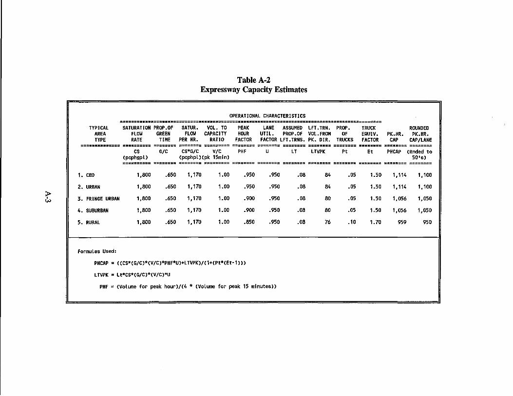
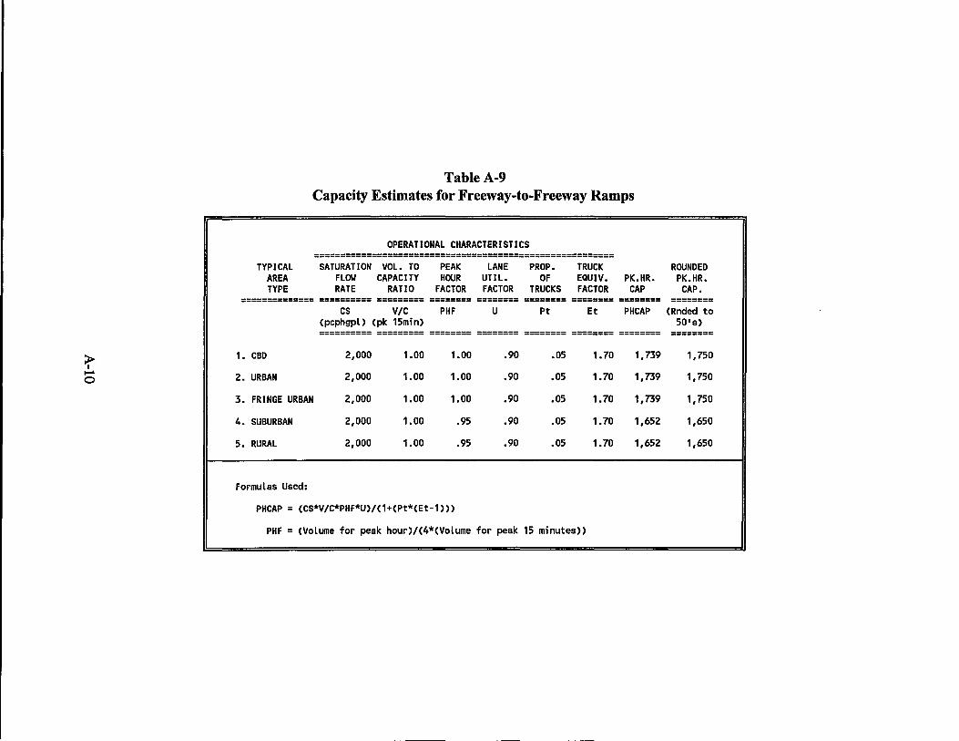
capacities developed for use in the detailed coding are summarized in Table 5. Tables A-7
through A-14 (of Appendix A) document the formulas and the typical parameter values applied
in the formulas to estimate the hourly capacities. The Transportation Planning and Programming
Division requested that 24-hour detailed networks also be developed and assigned for use in the
corridor analysis performed by the division. The 24-hour capacities for the detailed coding are
also summarized in Table 5. The capacities for the non-detailed portions of the network are the
same as those listed in Table 3 of this report. The detailed networks for each of the IH-35 design
alternatives prepared under this study were provided to TxDOT.
27
Table 5 Austin Detailed Network Capacities
24-HOUR CAPACITIES HOURLY CAPACITIES Link =============================== ===============================
Functional Area Speeds Num. Capacity! Front. Rd. Num. Capacity! Front. Rd. Class Type kph (mph) Lanes x Lane + Capacity Lanes x Lane + Capacity
========== ======== ========= =============================== --------------------------------------------------------------Normal 1 72.5 (45.0) n x 19000 n x 1,950 Freeway 2 72.5 (45.0) n x 22750 n x 1,950 Main Lanes 3 80.5 (50.0) n x 22750 n x 1,950
4 88.6 (55.0) n x 20125 n x 1,850 5 96.6 (60.0) n x 12000 n x 1,700
Elevated & 1 77.3 (48.0) n x 19975 n x 2,050 Depressed 2 77.3 (48.0) n x 23925 n x 2,050 Freeway 3 85.3 (53.0) n x 23925 n x 2,050 Main Lanes 4 93.4 (63.0) n x 21225 n x 1,950
5 101.0 (63.0) n x 12700 n x 1,800
Freeway 1 64.4 (40.0) n x 17050 n x 1,750 to 2 64.4 (40.0) n x 20425 n x 1,750 Freeway 3 72.5 (45.0) n x 20425 n x 1,750 Ramps 4 72.5 (45.0) n x 17950 n x 1,650
5 72.5 (45.0) n x 11650 n x 1,650
Collector! 1 56.4 (35.0) n x 17050 n x 1,750 Distributor 2 56.4 (35.0) n x 20425 n x 1,750 (CD) Lanes 3 64.4 (40.0) n x 20425 n x 1,750
4 64.4 (40.0) n x 17950 n x 1,650 5 64.4 (40.0) n x 11650 n x 1,650
HOV 1 96.6 (60.0) Not Appl icable n x 2,050 Lanes 2 96.6 (60.0) Not Appl icable n x 2,050
3 96.6 (60.0) Not Appl icable n x 2,050 4 96.6 (60.0) Not Appl icable n x 2,050 5 105.0 (65.0) Not Applicable n x 2,050
Normal 1 48.3 (30.0) n x 15725 n x 1,500 Ramps 2 48.3 (30.0) n x 16575 n x 1,500
3 56.4 (35.0) n x 16200 n x 1,500 4 64.4 (40.0) n x 15050 n x 1,500 5 72.5 (45.0) n x 10825 n x 1,500
Collector! 1 48.3 (30.0) n x 16525 n x 1,575 Distributor 2 48.3 (30.0) n x 17400 n x 1,575 Lanes to 3 56.4 (35.0) n x 17025 n x 1,575 Surface 4 56.4 (35.0) n x 15800 n x 1,575 Streets 5 56.4 (35.0) n x 11375 n x 1,575
HOV 1 48.3 (30.0) Not Applicable n x 1,575 Ramps 2 48.3 (30.0) Not Applicable n x 1,575
3 56.4 (35.0) Not Applicable n x 1,575 4 56.4 (35.0) Not Applicable n x 1,575 5 56.4 (35.0) Not Applicable n x 1,575
Frontage 1 40.3 (25.0) n x 7975 n x 710 Roads 2 48.3 (30.0) n x 7425 n x 710
3 56.4 (35.0) n x 7450 n x 750 4 64.4 (40.0) n x 6900 n x 750 5 80.5 (50.0) n x 5525 n x 750
28
DETAILED NETWORK ASSIGNMENTS
Both morning and afternoon peak-hour capacity restraint assignments and a 24-hour
capacity restraint assignment were performed using the detailed networks developed for each
design alternative studied. These 2020 assignments were performed using the ASSIGN SELF
BALANCING Routine in the Texas Large Network Package. The new equilibrium assignment
option (2) was used for these assignments. Six iterations were performed for each assignment.
The results for the three assignments performed for each design alternative studied were provided
to TxDOT.
PREPARATION OF POSTED ASSIGNMENT VOLUMES
The link data used for each assignment were converted from Texas Package format to
TRANPLAN format. The equilibrium assignment results were inserted in the TRANPLAN link
data in the fields normally used for the counted volumes. The TRANPLAN software was then
used to plot the networks with the assigned volumes posted. The posted network plots along with
the TRANPLAN data were transmitted to TxDOT.
FREQI0 APPLICATIONS
This section documents the use of FREAK in the analysis of improvements to the IH-35
freeway corridor. An explanation of the FREQI0 model is included as well as a discussion of
how models were developed for IH-35 and the measures of effectiveness (MOEs) which were
used. This section also discusses the methodology used to convert the output from the
TRANPLAN model into input data for the FREQI0 program.
FREQI0 Program
FREQ 10 is the tenth in a series of computer freeway simulation models that were
developed at the Institute of Transportation Studies (ITS), University of California, Berkeley. The
program allows simulation of traffic operations given a set of input parameters. Several different
measures of effectiveness (MOEs) are produced which provide the user with quantitative data to
compare various alternative freeway configurations.
29
Input Requirements
There are two types of input required for the FREQ 1 0 model -- demand characteristics and
freeway characteristics. In general, these characteristics require the following data:
Demand characteristics O-D patterns, vehicle occupancy levels, distribution of
Entrance and exit ramp volume counts and freeway mainlane volume counts are used as
input information to build a synthetic O-D trip matrix. Total entry volumes are apportioned to
downstream exit ramps in proportion to the volumes on those exit ramps.
Vehicle mix and vehicle occupancy are also required for freeway mainlane modeling.
Proportions of single occupant, double occupant, three or more occupant cars and buses in the
traffic stream are required for each entrance ramp.
Freeway Characteristics
Freeway characteristics quantify the supply side of the freeway system. The modeled
length of mainlane freeway is governed by: 1) a maximum of 40 freeway subsections; or 2) a
maximum of 20 input or 20 output locations. A subsection is defmed as a point of demand change
(entrance or exit ramp) or a geometric change (e.g., lane drop/addition, large gradient change,
etc.) The user must also supply (for each subsection) the number of lanes, the mainlane capacity,
gradient, curvature, speed versus flow relationship, ramp characteristics, and percentage of trucks.
Another limitation of FREQI0 is the maximum of 24 time periods, which, when used in 15-
minute increments, limits the model length to 6 hours. This is sufficient to encompass freeway
operations during a single peak period in the peak direction.
These data needs have been satisfied utilizing recording traffic counters, manual mainlane
traffic counts, and travel time and speed studies. The traffic counts are recorded at 15-minute
increments, and the travel time runs are started at 15-minute intervals. Some of the data are
30
generally available from area planning agencies, but the detailed count and travel speed
information is usually too expensive for those agencies to collect on a regular basis.
Modeling Assumptions
The FREQI0 program makes certain assumptions in order to operate effectively and
efficiently. It assumes that freeway operations can be simulated by ignoring any randomness in
traffic behavior and the behavior of individual vehicles. The program operating procedure
transfers demand downstream instantly at the beginning of each time period unless demand
exceeds capacity. This process greatly reduces computing time and is sufficiently accurate for
almost all situations. It does not provide the detailed accounting of individual vehicle movements
provided by more microscopic models and required in some traffic engineering analyses.
If demand exceeds capacity in a particular time period/subsection combination, traffic is
stored on upstream entrance ramps or upstream freeway subsections. These vehicles become part
of the demand for the following time period and are counted in the travel time delay estimate.
The model, however, does not shift the mode of trips or the entry location, and it assumes that
traffic demand and roadway capacity remain constant over a time period.
Freeway HOV Lane Analysis with FREQlO
The input data are used to calibrate the model to existing freeway conditions using the
speed and congestion contours derived from the travel time runs. The model information is
adj~sted to match the observed information by changing subsection capacity in the congested
areas. The level of precision is well within that of the input data and is consistent with the
ultimate use of the FREQI0 model in this study.
The FREQI0 model provides considerable data that permit quantitative comparison of
alternatives. The measures of effectiveness (MOEs) included in the output are: 1) vehicle-hours
and passenger hours of travel on the freeway; 2) vehicle hours and passenger hours of ramp delay;
3) total vehicle hours and passenger hours; 4) total vehicle miles and passenger miles; 5) average
vehicle speed; and 6) total fuel consumption.
31
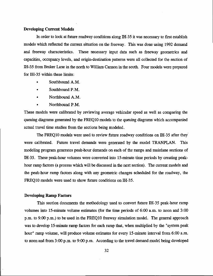
Developing Current Models
In order to look at future roadway conditions along IH-35 it was necessary to fIrst establish
models which reflected the current situation on the freeway. This was done using 1992 demand
and freeway characteristics. These necessary input data such as freeway geometrics and
capacities, occupancy levels, and origin-destination patterns were all collected for the section of
IH-35 from Braker Lane in the north to William Cannon in the south. Four models were prepared
for IH-35 within these limits:
• Southbound A.M.
• Southbound P.M.
• Northbound A.M.
• Northbound P.M.
These models were calibrated by reviewing average vehicular speed as well as comparing the
queuing diagrams generated by the FREQlO models to the queuing diagrams which accompanied
actual travel time studies from the sections being modeled.
The FREQIO models were used to review future roadway conditions on IH-35 after they
were calibrated. Future travel demands were generated by the model TRANPLAN. This
modeling program generates peak-hour demands on each of the ramps and mainlane sections of
IH-35. These peak-hour volumes were converted into I5-minute time periods by creating peak
hour ramp factors (a process which will be discussed in the next section). The current models and
the peak-hour ramp factors along with any geometric changes scheduled for the roadway, the
FREQIO models were used to show future conditions on IH-35.
Developing Ramp Factors
This section documents the methodology used to convert future IH-35 peak-hour ramp
volumes into I5-minute volume estimates (for the time periods of 6:00 a.m. to noon and 3:00
p.m. to 9:00 p.m.) to be used in the FREQlO freeway simulation model. The general approach
was to develop I5-minute ramp factors for each ramp that, when multiplied by the "system peak
hour" ramp volume, will produce volume estimates for every I5-minute interval from 6:00 a.m.
to noon and from 3:00 p.m. to 9:00 p.m. According to the travel demand model being developed
32
for the year 2020, the morning and evening peak hours of travel for the Austin area will occur
from 7:00 a.m. to 8:00 a.m and from 5:00 p.m. to 6:00 p.m.; peak hours varied on the ramps on
IH-35.
Preliminaty Ramp Grouping
The study limits for the llI-3S FREQlO analyses were determined to be from north of the
Braker exit to south of the Riverside exit in the southbound direction and from south of William
Cannon entrance to north of the US 290 exit in the northbound direction for the morning analyses.
The 57 ramps within the llI-3S study limits were divided into groups according to the direction
(northbound or southbound), the type of ramp (entrance or exit), and the capacity of the ramp.
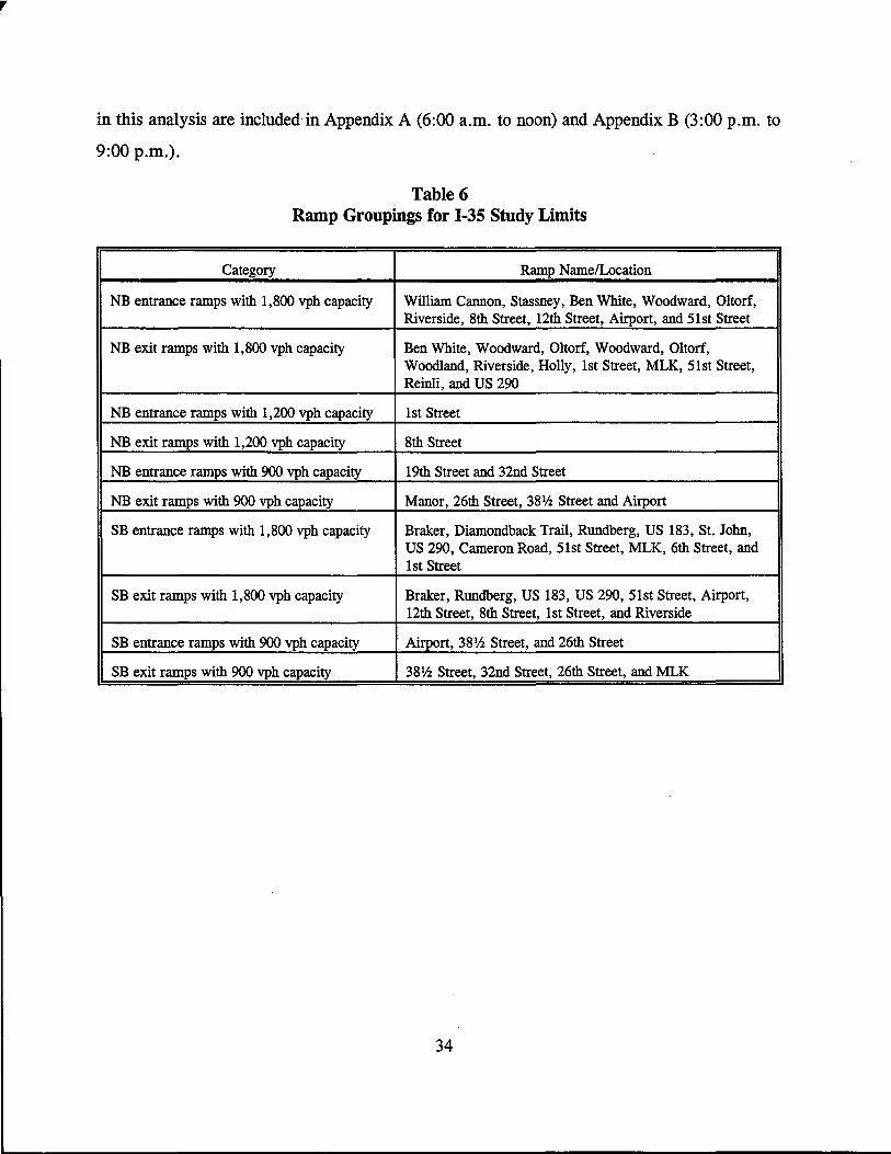
This preliminary sorting process resulted in the 10 ramp groups shown in Table 6.
Data Reduction
After the ramps were divided into the 10 groups listed in Table 6, they had to be divided
further in order to group ramps with similar IS-minute ramp factors. This was done by utilizing
the historic ramp counts for each of the 57 ramps in the study to calculate the ratio of the 15-
minute volume to the system's peak-hour volume (PHV) for each of the 24 IS-minute intervals.
First, a statistical analysis was performed on each ramp data set. This procedure consisted of
examining the minimum value, maximum value, average, median, range, standard deviation, and
correlation coefficient in order to identify ramps with similar ratios within the same group for
each of the 6-hour periods (morning and evening). Once the ramps were reduced to smaller
groups, their ratios were plotted for each IS-minute period. From these plots, it could be further
determined which ramps could be grouped together for the ramp factor calculations. Example
calculations for 12th Street, 8th Street, 1st Street, and Riverside ramps from 6:00 a.m. to noon
(which are part of the southbound exit ramp group with 1,800 vph) are included in Table 7. It
should be noted that the values included in Table 7 reflect the IS-minute ramp factors in
percentage form. Note that the averages, standard deviations (0), and correlation coefficients (r)
(which were some of the statistics used to reduce the groups) do not vary greatly. The general
relationship between these four ramps is illustrated in Figure 1. The remaining plots developed
33
,.
in this analysis are included'in Appendix A (6:00 a.m. to noon) and Appendix B (3:00 p.m. to
9:00 p.m.).
Table 6 Ramp Groupings for 1-35 Study Limits
Category Ramp Name/Location
NB entrance ramps with 1,800 vph capacity William Cannon, Stassney, Ben White, Woodward, Oltorf, Riverside, 8th Street, 12th Street, Airport, and 51st Street
NB exit ramps with 1,800 vph capacity Ben White, Woodward, Oltorf, Woodward, Oltorf, Woodland, Riverside, Holly, 1st Street, MLK, 51st Street, Reinli, and US 290
NB entrance ramps with 1,200 vph capacity 1st Street
NB exit ramps with 1,200 vph capacity 8th Street
NB entrance ramps with 900 vph capacity 19th Street and 32nd Street
NB exit ramps with 900 vph capacity Manor, 26th Street, 38% Street and Airport
SB entrance ramps with 1,800 vph capacity Braker, Diamondback Trail, Rundberg, US 183, St. John, US 290, Cameron Road, 51st Street, MLK, 6th Street, and 1st Street
SB exit ramps with 1,800 vph capacity Braker, Rundberg, US 183, US 290, 51st Street, Airport, 12th Street, 8th Street, 1st Street, and Riverside
SB entrance ramps with 900 vph capacity Airport, 381h Street, and 26th Street
SB exit ramps with 900 vph capacity 381h Street, 32nd Street, 26th Street, and MLK
34
Table 7 Statistical Analysis of a Sample Group of Southbound Exit Ramps
Morning Evaluation Period
Southbound Exit Minimum Maximum Average Median
Standard Correlation Ramp Deviationl Coefficienr
12th Street 3.06 43.18 18.23 15.17 9.710 +0.1076
8th Street 5.42 33.67 17.48 16.13 6.572 +0.0676
1st Street 4.42 34.32 19.18 17.47 7.956 +0.2009
Riverside 5.29 31.88 20.10 20.94 6.941 +0.3292
Note: All values included above reflect the ramp factors in percentage form (Le., ramp factor x 100). lTbe standard deviation (0) is a measure of dispersion. It gives a numerical value representing the clustering tendency of the data.
2Tbe correlation coefficient (r) is a measure of the strength of the linear relationship between two
quantitative variables.
Ramp Factor Determination
Once the groups from Table 6 were reduced, the average ramp factors were determined.
Table 8 indicates the 15-minute volumes for each ramp and the weighted average (or ramp factor
[PHF]) for the 12th, 8th, 1st, and Riverside Streets southbound exit ramp grouping. These ramp
factors were calculated by using the 15-minute to system peak-hour volume (PMV) ratios (in
parentheses in the equations below) and the peak-hour volumes for each of the ramps in the group.
The average ramp factor was weighted according to the peak-hour volume ratios for each ramp.
The following example illustrates the determination of the ramp factor for the 7:45 to 8:00 a.m.
15-minute interval for the ramps shown in Table 8.
where: 0.271 = ramp factor for NB William Cannon entrance ramp for 7:15-7:30
a.m. (Table 10).
As with any automated calculation, a reasonableness check should always be made to
ensure that the 15-minute volumes are plausible. A good rule of thumb is no more than 500
vehicles per 15-minute interval for ramps with 1,800 vph capacity, no more than 330 vehicles per
interval for ramps with 1,200 ·vph capacity, and no more than 250 vehicles per interval for ramps
with 900 vph capacity. An example of a potential problem ramp is the SB Braker Exit where, due
to its relatively low historic volumes, an extremely high 15-minute ramp factor is obtained at time
period 8: 15 to 8:30 a.m.
It should be noted that the peak hour of the system and the peak hour of the individual
ramp will not always exactly coincide. The morning and evening peak hours of travel for the
system are from 7:00 a.m. to 8:00 a.m and 5:00 p.m. to 6:00 p.m. An individual ramp, however,
may have a peak-hour volume from 7:30 a.m. to 8:30 a.m or from 4:45 p.m. to 5:45 p.m. This
results in the sum of four consecutive 15-minute ramp factors potentially exceeding 1.0 outside
the 7:00 to 8:00 a.m. or 5:00 to 6:00 p.m. time periods. Nevertheless, the 15-minute Ramp
Factors should always be approximately 1.0 from 7:00 to 8:00 a.m. and from 5:00 to 6:00 p.m.
36
15-minute interval (a.m.)
6:00
6:15
6:30
6:45
7:00
7:15
7:30
7:45
8:00
8:15
8:30
8:45
9:00
9:15
9:30
9:45
10:00
10:15
10:30
10:45
11:00
11:15
11:30
11:45
Table 8 Example Ramp Factors for Southbound Exit Ramps
Morning Evaluation Period
Historical Ramp Factors l
12th Street 8th Street 1" Street Riverside
0.031 0.054 0.044 0.053
0.040 0.063 0.057 0.062
0.059 0.082 0.076 0.061
0.099 0.119 0.112 0.133
0.137 0.194 0.156 0.205
0.200 0.215 0.206 0.211
0.286 0.263 0.257 0.268
0.324 0.278 0.307 0.305
0.432 0.337 0.343 0.300
0.380 0.266 0.331 0.319
0.221 0.224 0.272 0.247
0.238 0.185 0.272 0.220
0.217 0.198 0.246 0.227
0.146 0.138 0.158 0.211
0.122 0.148 0.164 0.180
0.133 0.153 0.162 0.186
0.153 0.148 0.175 0.208
0.119 0.137 0.158 0.213
0.131 0.162 0.175 0.183
0.147 0.181 0.118 0.191
0.150 0.154 0.171 0.168
0.179 0.145 0.177 0.182
0.194 0.160 0.213 0.221
0.240 0.193 0.255 0.271
Weighted Average2
0.047
0.056
0.070
0.117
0.180
0.212
0.280
0.308
0.351
0.318
0.237
0.220
0.217
0.163
0.153
0.158
0.169
0.156
0.162
0.166
0.159
0.168
0.193
0.235
The ratio ofhistoncall5-mmute volumes to the peak-hour volume (7-8 a.m.), these ratIos were calculated for data obtained from 1988 to 1991.
lrhe average (weighted by volume) ramp factor for the group of similar ramps, in this case, southbound exit ramps at 1st Street, 8th Street, 12th Street and Riverside. This value represents the factor by which to multiply the future (2020) peak-hour volume to obtain IS-minute ramp volume estimates for the year 2020 to be used in the FREQ model.
37
w 00
Table 9 IS-Minute Ramp Factors for Southbound IH-3S, Morning Evaluation Period
Entrance Ramps
TIME Braker DBTI US 183
(am) St Jolm Aiw.0rt MLK Rundberg Cameron2 US 290 3 .5 26th 6th Braker
51st 1st
6:00 .074 .063 .065 .077 .038 .070 .038
6:15 .072 .075 .069 .082 .071 .077 .086
6:30 .103 .078 .099 .113 .062 .099 .143
6:45 .167 .110 .141 .107 .091 .116 .143
7:00 .205 .162 .177 .183 .105 .199 .286
7:15 .270 .218 .240 .224 .262 .235 .229
7:30 .277 .248 .257 .255 .305 .230 .229
7:45 .247 .365 .309 .376 .324 .328 .238
8:00 .185 .355 .282 .592 .381 .322 .556
8:15 .186 .248 .247 .543 .362 .336 .8153
8:30 .204 .227 .227 .476 .229 .283 .400
8:45 .206 .195 .243 .460 .281 .346 .333
9:00 .171 .170 .216 .389 .271 .340 .381
9:15 .144 .138 .196 .366 .290 .306 .229
9:30 .152 .138 .199 .323 .309 .315 .257
9:45 .135 .136 .194 .378 .262 .262 .276
10:00 .122 .146 .154 .377 .262 .377 .276
10:15 .128 .120 .171 .499 .313 .346 .238
10:30 .114 .124 .174 .439 .390 .343 .305
10:45 .137 .134 .179 .411 .295 .345 .343
11:00 .118 .135 .166 .454 .469 .462 .229
11:15 .143 .154 .169 .489 .400 .400 .362
11:30 .131 .142 .197 .489 .448 .487 .248
11:45 .130 .148 .223 .535 .457 .493 .371
lDiamondback Trail Entrance Ramp. This ramp is designated as the Braker entrance in the FREQ model. 2Cameron Road Turnaround Entrance Ramp. This ramp is designated as US 290 entrance in the FREQ model. 3Check calculated IS-minute volume for reasonableness.
Exit Ramps
US 183 Rundberg US 290 Airport 38.5
51st
.060 .060 .156 .039
.063 .063 .124 .048
.097 .087 .115 .059
.124 .152 .184 .135
.274 .226 .250 .167
.310 .248 .252 .200
.232 .286 .255 .252
.184 .232 .238 .383
.213 .300 .262 .415
.198 .221 .251 .281
.189 .215 .236 .232
.138 .177 .267 .239
.149 .174 .224 .223
.110 .135 .203 .194
.114 .157 .216 .265
.106 .149 .200 .199
.068 .141 .216 .171
.090 .144 .170 .174
.095 .139 .229 .220
.097 .185 .219 .227
.103 .151 .227 .272
.062 .160 .223 .214
.089 .182 .212 .214
.052 .188 .194 .272
12th 32nd 8th 26th MLK 1st
River
.044 .009 .047
.059 .020 .056
.075 .035 .070
.154 .080 .117
.174 .156 .180
.222 .170 .212
.268 .322 .280
.331 .352 .308
.316 .261 .351
.286 .185 .318
.249 .187 .237
.333 .141 .220
.225 .120 .217
.195 .061 .163
.185 .091 .153
.188 .094 .158
.167 .100 .169
.149 .056 .156
.148 .098 .162
.150 .091 .166
.119 .054 .159
.128 .065 .168
.125 .077 .193
.143 .101 .235
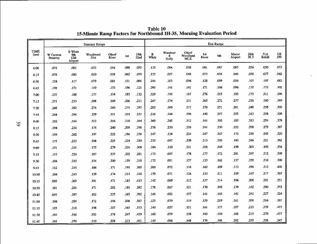
Table 10 15-Minute Ramp Factors for Northbound IH-35, Morning Evaluation Period
Entrance Ramps Exit Ramps
TIME B White Woodwar Oltorf (am) W Cannon 8th Woodward Oltorf 1st 19th B d Woodland 1st 8th Manor 26th 51st US Stassney 12th 51st River 32nd White Holly MLK River Airport 38.5 Reinli 290
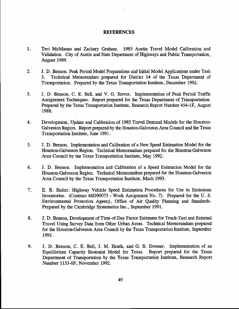
1. Teri McManus and Zachary Graham. 1985 Austin Travel Model Calibration and Validation. City of Austin and State Department of Highways and Public Transportation, August 1989.
2. J. D. Benson. Peak Period Model Preparations and Initial Model Applications under Task 3. Technical Memorandum prepared for District 14 of the Texas Department of Transportation. Prepared by the Texas Transportation Institute, December 1992.
3. J. D. Benson, C. E. Bell, and V. G. Stover. Implementation of Peak Period Traffic Assignment Techniques. Report prepared for the Texas Department of Transportation. Prepared by the Texas Transportation Institute, Research Report Number 454-1F, August 1988.
4. Development, Update and Calibration of 1985 Travel Demand Models for the HoustonGalveston Region. Report prepared by the Houston-Galveston Area Council and the Texas Transportation Institute, June 1991.
5. J. D. Benson. Implementation and Calibration of a New Speed Estimation Model for the Houston-Galveston Region. Technical Memorandum prepared for the Houston-Galveston Area Council by the Texas Transportation Institute, May 1992.
6. J. D. Benson. Implementation and Calibration of a Speed Estimation Model for the Houston-Galveston Region. Technical Memorandum prepared for the Houston-Galveston Area Council by the Texas Transportation Institute, Mach 1993.
7. E. R. Ruiter. Highway Vehicle Speed Estimation Procedures for Use in Emissions Inventories. (Contract 68D90073 - Work Assignment No.7). Prepared for the U. S. Environmental Protection Agency, Office of Air Quality Planning and Standards. Prepared by the Cambridge Systematics Inc., September 1991.
8. J. D. Benson, Development of Time-of-Day Factor Estimates for Truck-Taxi and External Travel Using Survey Data from Other Urban Areas. Technical Memorandum prepared for the Houston-Galveston Area Council by the Texas Transportation Institute, September 1991.
9. J. D. Benson, C. E. Bell, J. M. Heath, and G. B. Dresser. Implementation of an Equilibrium Capacity Restraint Model for Texas. Report prepared for the Texas Department of Transportation by the Texas Transportation Institute, Research Report Number 1153-6F, November 1992.
49
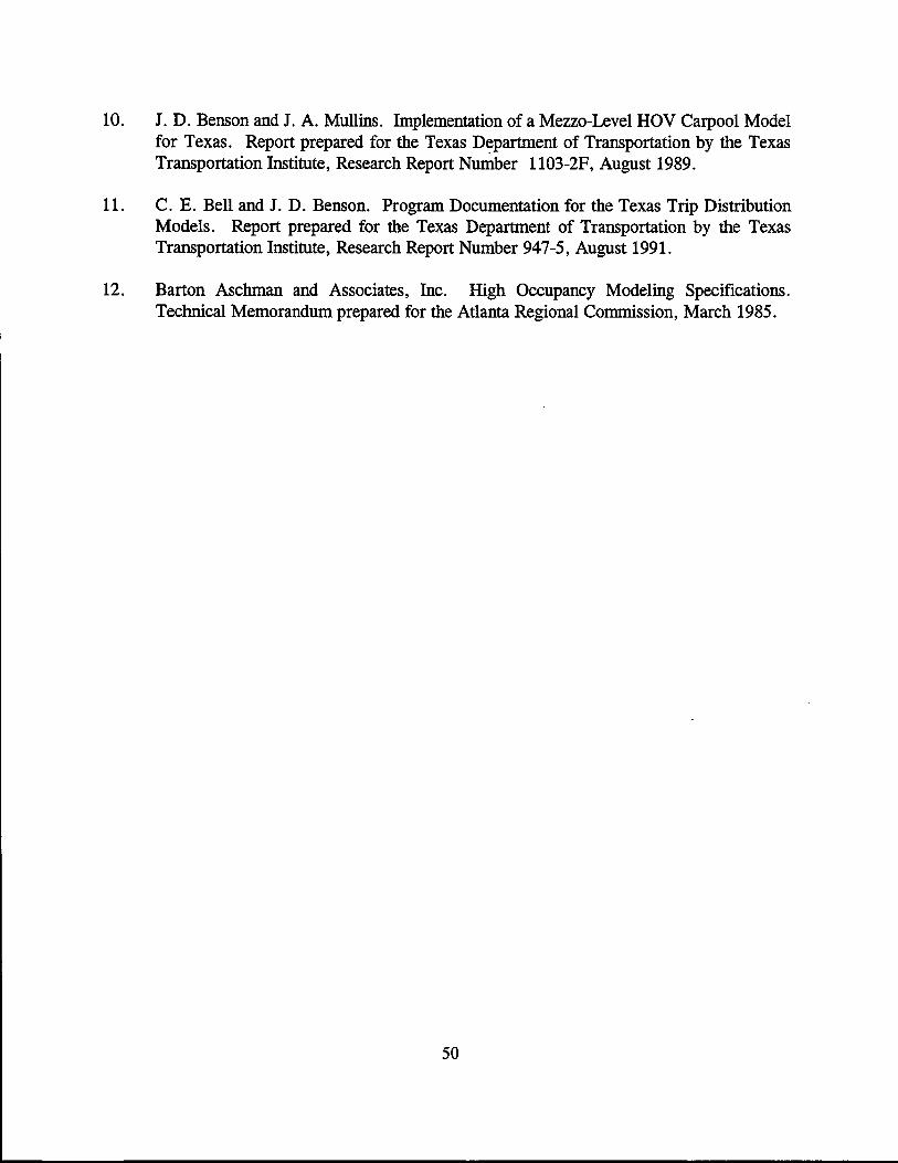
10. J. D. Benson and J. A. Mullins. Implementation of a Mezzo-Level HOV Carpool Model for Texas. Report prepared for the Texas Department of Transportation by the Texas Transportation Institute, Research Report Number 1103-2F, August 1989.
11. C. E. Bell and J. D. Benson. Program Documentation for the Texas Trip Distribution Models. Report prepared for the Texas Department of Transportation by the Texas Transportation Institute, Research Report Number 947-5, August 1991.
12. Barton Aschman and Associates, Inc. High Occupancy Modeling Specifications. Technical Memorandum prepared for the Atlanta Regional Commission, March 1985.
50
APPENDIX A: ESTIl\1ATION OF HOURLY CAPACITIES
FOR AUSTIN IDGHW AY NETWORKS
The purpose of this appendix is to document the formulas and parameters used in
estimating the hourly capacities for the peak-hour networks used in this study. Tables A-I
through A-6 summarize the capacity calculations for the functional classifications used in the ATS
highway networks. The detailed coding techniques employed in the IH-35 analyses required the
delineation of additional functional classifications. Tables A-7 through A-14 summarize the
capacity calculations for the hourly capacities used in the detailed coding of the IH-35 alternatives.
TYPICAL SATURATION VOL. TO PEAK LANE PROP. TRUCK ROUNDED AREA FLOW CAPACITY HOUR UTIL. OF EQUIV. PK.HR. PK.HR. TYPE RATE RATIO FACTOR FACTOR TRUCKS FACTOR CAP CAP.
============== ========== ========= ======== ======== ======== ======== ======== ----------------CS VIC PHF U Pt Et PHCAP (Rnded to
TYPICAL SATURATION PROP.OF SATUR. VOL. TO PEAK LANE ASSUMED LFT. TRN. PROP. TRUCK ROUNDED AREA FLOW GREEN FLOW CAPACITY HOUR UTIL. PROP.OF VOL. FROM OF EQUIV. PK.HR. PK.HR. TYPE RATE TIME PER HR. RATIO FACTOR FACTOR LFT. TRNS. PK. DIR. TRUCKS FACTOR CAP CAP/LANE
============== ========== ======== ======== ========= ======== ======== ======== ======== ======== ======== ======== ======== CS G/C CS*G/C VIC PHF U LT LTVPK Pt Et PHCAP (Rnded to
TYPICAL SATURATION PROP.OF SATUR. VOL. TO PEAK LANE ASSUMED LFT.TRN. PROP. TRUCK ROUNDED AREA FLOW GREEN FLOW CAPACITY HOUR UTIL. PROP.OF VOL. FROM OF EQUIV. PK.HR. PK.HR. TYPE RATE TIME PER HR. RATIO FACTOR FACTOR LFT.TRNS. PK. DIR. TRUCKS FACTOR CAP. CAP/LANE
============== ========== ======== ======== ========= ======== ======== ======== ======== ======== ======== ======== ======== CS G/C CS*G/C VIC PHF U LT LTVPK Pt Et PHCAP (Rnded to
(pcphgpl) (pcphpl )(pk 15min) per lane per lane 10 1s) ========== ======== ======== ========= ======== ======== ======== ======== ======== ======== ======== ========
TYPICAL SATURATION PROP.OF SATUR. VOL. TO PEAK LANE PROP. IN ASSUMED LFT. TRN. PROP. TRUCK ROUNDED AREA FLOW GREEN FLOW CAPACITY HOUR UTIL. PK. DIR. PROP.OF VOL. FROM OF EQUIV. PK.HR. PK.HR. TYPE RATE TIME PER HR. RATIO FACTOR FACTOR IN PK.HR.LFT.TRNS.OPP. DIR. TRUCKS FACTOR CAP. CAP/LANE
============== ========== ======== ======== ========= ======== ======== ======== ======== ======== ======== ======== ======== ======== CS G/C CS*G/C VIC PHF U D LT LTVOP Pt Et PHCAP (Rnded to
LTVOP = (Lt*CS*(G/C)*(V/C)*U)*((1-D)/D)*(Average number of lanes in opposite direction) Average number of lanes in opposite direction assumed to be 2.5 for major arterials
PHF = (Volume in the peak hour)/( 4 * (Volume in the peak 15 minutes»
TYPICAL SATURATION PROP.OF SATUR. VOL. TO PEAK LANE PROP. IN ASSUMED LFT.TRN. PROP. TRUCK ROUNDED AREA FLOW GREEN FLOW CAPACITY HOUR UTIL. PK. DIR. PROP.OF VOL. FROM OF EQUIV. PK.HR. PK.HR. TYPE RATE TIME PER HR. RATIO FACTOR FACTOR IN PK.HR.LFT.TRNS.OPP. DIR. TRUCKS FACTOR CAP. CAP/LANE
============== ========== ======== ======== ========= ======== ======== ======== ======== ======== ======== ======== ======== =======: CS G/C CS*G/C VIC PHF U 0 LT LTVOP Pt Et PHCAP (Rnded to
LTVOP = (Lt*CS*(G/C)*(V/C)*U)*«1-D)/D)*(AVerage number of Lanes in opposite direction) Average number of Lanes in opposite direction assumed to be 1.5 for minor arteriaLs
PHF = (VoLume in the peak hour)/( 4 * (VoLume in the peak 15 minutes»
TYPICAL SATURATION PROP.OF SATUR. VOL. TO PEAK LANE PROP. IN ASSUMED LFT.TRN. PROP. TRUCK ROUNDED AREA FLOW GREEN FLOW CAPACITY HOUR UTiL. PK. DIR. PROP.OF VOL. FROM OF EQUIV. PK.HR. PK.HR. TYPE RATE TIME PER HR. RATIO FACTOR FACTOR IN PK.HR.LFT.TRNS.OPP. DIR. TRUCKS FACTOR CAP. CAP/LANE
======:======= ========== ======== ======== ======:== ======== ======== ======== ======== ======== ======== ======== ======== ======== CS G/C CS*G/C VIC PHF U 0 LT LTVOP Pt Et PHCAP (Rnded to
LTVOP = (Lt*CS*(G/C)*(V/C)*U)*«1-D)/D)*(Average number of lanes in opposite direction) Average number of lanes in opposite direction assumed to be 1.5 for minor arterials
PHF = (Volume in the peak hour)/( 4 * (Volume in the peak 15 minutes»
~ 00
TableA-7 Capacity Estimates for Normal Freeway Main Lanes
TYPICAL SATURATION PROP.OF SATUR. VOL. TO PEAK LANE ASSUMED LFT. TRN. PROP. TRUCK ROUNDED AREA FLOW GREEN FLOW CAPACITY HOUR UTiL. PROP.OF VOL. FROM OF EQUIV. PK.HR. PK.HR. TYPE RATE TIME PER HR. RATIO FACTOR FACTOR LFT.TRNS. PK. DIR. TRUCKS FACTOR CAP. CAP/LANE
============== ========== ======== ======== ========= ======== ======== ======== ======== ======== ======== ======== ======== CS G/C CS*G/C VIC PHF U LT LTVPK Pt Et PHCAP (Rnded to
(pcphgpl) (pcphpl )(pk 15min) per lane per lane 10's) ========== ======== ======== ========= ======== ======== ======== ======== ======== ======== ======== ========


![Whirlpool Delta Awm 5080 [ET]](https://static.documents.pub/doc/80x56/5480135cb4795979578b45f0/whirlpool-delta-awm-5080-et.jpg)


