Tutorial — FM 2008

Formal Methods and Signal Processing

Raymond Boute, INTEC — Ghent University Tuesday, 2008-05-27

09:00–09:20 0. Motivation: synergy FM-SP; value of defect-free formalisms

Part I — Unifying the mathematics of SP and FM09:20–09:40 1. Review of the basics and outline of the formalism used09:40–10:10 2. Inspiration from SP to FM: functions and functionals10:10–10:30 3. Calculation with predicates and quantifiers for engineers

10:30–11:00 (Half-hour break)

Part II — Application examples to modeling in SP and FM11:00–11:40 4. Predicate calculus and generic functionals applied to classical SP11:40–11:45 5. Brief intermezzo about endosemantic functions11:45–12:05 6. Modeling programs by program equations12:05–12:25 7. Reasoning about temporal behavior by temporal operators12:25–12:30 8. Final considerations

0

0 Motivation: synergy FM-SP; defect-free formalisms

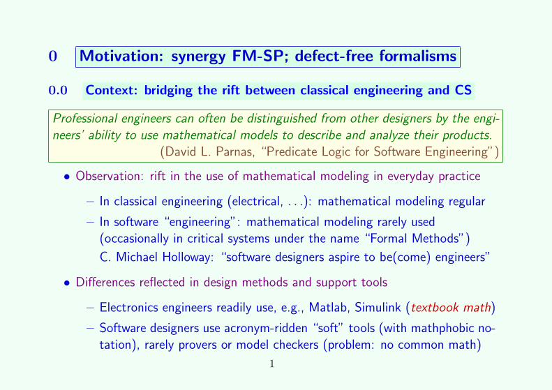
0.0 Context: bridging the rift between classical engineering and CS

Professional engineers can often be distinguished from other designers by the engi-neers’ ability to use mathematical models to describe and analyze their products.

(David L. Parnas, “Predicate Logic for Software Engineering”)

• Observation: rift in the use of mathematical modeling in everyday practice

– In classical engineering (electrical, . . .): mathematical modeling regular

– In software “engineering”: mathematical modeling rarely used(occasionally in critical systems under the name “Formal Methods”)

C. Michael Holloway: “software designers aspire to be(come) engineers”

• Differences reflected in design methods and support tools

– Electronics engineers readily use, e.g., Matlab, Simulink (textbook math)

– Software designers use acronym-ridden “soft” tools (with mathphobic no-tation), rarely provers or model checkers (problem: no common math)

1

0.1 Motivation: exploiting the many synergies between SP and FM

• Observations about SP

a. + Traditionally mathematics-intensive; mathematical modeling is regularengineering practice — a role model for [wannabe] software engineers!

− Still many defective formulations (examples shown soon)

b. + Broadened from analog models/circuits: now also multidimensional in-formation and algorithms implemented in software

− Models for signals and systems are well-known, for algorithms and soft-ware largely unexploited by the SP community

• Observations about FM

c. Growing importance of SP ⇒ more involvement of software engineers

Consequence: future SWE requires signals and systems background(already observed by Parnas nearly two decades ago)

Establishing this background via FM provides significant synergy.

2

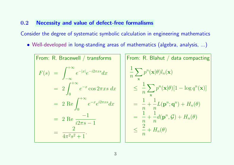
0.2 Necessity and value of defect-free formalisms

Consider the degree of systematic symbolic calculation in engineering mathematics

• Well-developed in long-standing areas of mathematics (algebra, analysis, ...)

From: R. Bracewell / transforms

F (s) =

∫ +∞

−∞e−|x|e−i2πxsdx

= 2

∫ +∞

0e−x cos 2πxs dx

= 2 Re

∫ +∞

0e−xei2πxsdx

= 2 Re−1

i2πs− 1

=2

4π2s2 + 1.

From: R. Blahut / data compacting

1

n

∑x

pn(x|θ)ln(x)

≤ 1

n

∑x

pn(x|θ)[1− log qn(x)]

=1

n+

1

nL(pn;qn) +Hn(θ)

=1

n+

1

nd(pn,G) +Hn(θ)

≤ 2

n+Hn(θ)

3

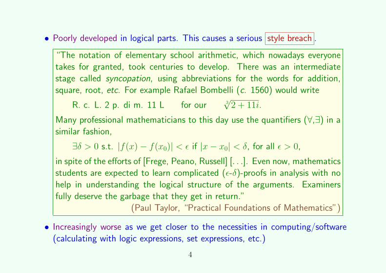
• Poorly developed in logical parts. This causes a serious style breach .

“The notation of elementary school arithmetic, which nowadays everyonetakes for granted, took centuries to develop. There was an intermediatestage called syncopation, using abbreviations for the words for addition,square, root, etc. For example Rafael Bombelli (c. 1560) would write

R. c. L. 2 p. di m. 11 L for our 3√

2 + 11i.

Many professional mathematicians to this day use the quantifiers (∀,∃) in asimilar fashion,

∃δ > 0 s.t. |f(x)− f(x0)| < ε if |x− x0| < δ, for all ε > 0,

in spite of the efforts of [Frege, Peano, Russell] [. . .]. Even now, mathematicsstudents are expected to learn complicated (ε-δ)-proofs in analysis with nohelp in understanding the logical structure of the arguments. Examinersfully deserve the garbage that they get in return.”

(Paul Taylor, “Practical Foundations of Mathematics”)

• Increasingly worse as we get closer to the necessities in computing/software(calculating with logic expressions, set expressions, etc.)

4

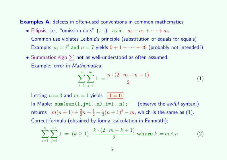
Examples A: defects in often-used conventions in common mathematics

• Ellipsis, i.e., “omission dots” (. . .) as in a0 + a1 + · · ·+ an

Common use violates Leibniz’s principle (substitution of equals for equals)

Example: ai = i2 and n = 7 yields 0 + 1 + · · ·+ 49 (probably not intended!)

• Summation sign∑

not as well-understood as often assumed.

Example: error in Mathematica:n∑

i=1

m∑j=i

1 =n · (2 ·m− n+ 1)

2(1)

Letting n := 3 and m := 1 yields 1 = 0

In Maple: sum(sum(1,j=i..m),i=1..n); (observe the awful syntax!)

returns m(n+ 1) + 32n+ 1

2 −12(n+ 1)2 −m, which is the same as (1).

Correct formula (obtained by formal calculation in Funmath):n∑

i=1

m∑j=i

1 = (k ≥ 1) · k · (2 ·m− k + 1)

2where k :=m∧n (2)

5

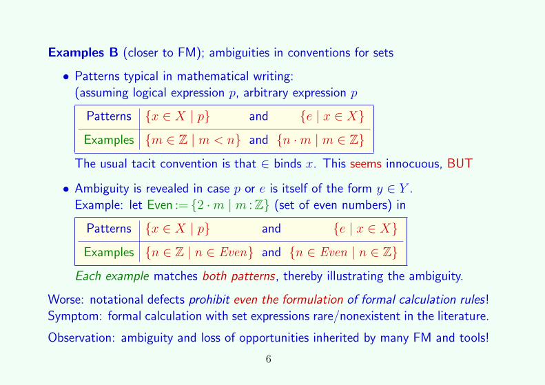
Examples B (closer to FM); ambiguities in conventions for sets

• Patterns typical in mathematical writing:(assuming logical expression p, arbitrary expression p

Patterns {x ∈ X | p} and {e | x ∈ X}

Examples {m ∈ Z | m < n} and {n ·m | m ∈ Z}

The usual tacit convention is that ∈ binds x. This seems innocuous, BUT

• Ambiguity is revealed in case p or e is itself of the form y ∈ Y .Example: let Even := {2 ·m | m : Z} (set of even numbers) in

Patterns {x ∈ X | p} and {e | x ∈ X}

Examples {n ∈ Z | n ∈ Even} and {n ∈ Even | n ∈ Z}

Each example matches both patterns, thereby illustrating the ambiguity.

Worse: notational defects prohibit even the formulation of formal calculation rules!Symptom: formal calculation with set expressions rare/nonexistent in the literature.

Observation: ambiguity and loss of opportunities inherited by many FM and tools!

6

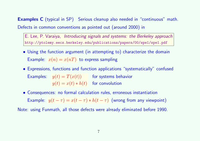
Examples C (typical in SP) Serious cleanup also needed in “continuous” math.

Defects in common conventions as pointed out (around 2000) in

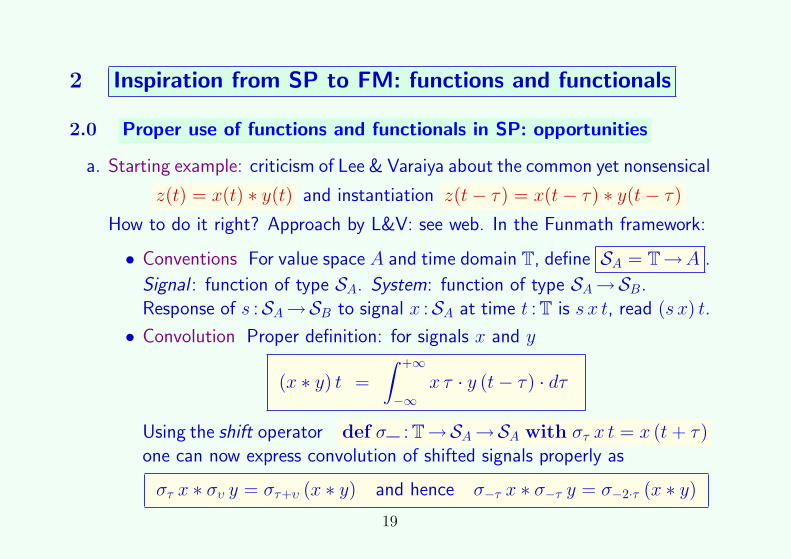
E. Lee, P. Varaiya, Introducing signals and systems: the Berkeley approachhttp://ptolemy.eecs.berkeley.edu/publications/papers/00/spe1/spe1.pdf

• Using the function argument (in attempting to) characterize the domain

Example: x(n) = x(nT ) to express sampling

• Expressions, functions and function applications “systematically” confused

Examples: y(t) = T (x(t)) for systems behavior

y(t) = x(t) ∗ h(t) for convolution

• Consequences: no formal calculation rules, erroneous instantiation

Example: y(t− τ) = x(t− τ) ∗ h(t− τ) (wrong from any viewpoint)

Note: using Funmath, all those defects were already eliminated before 1990.

7

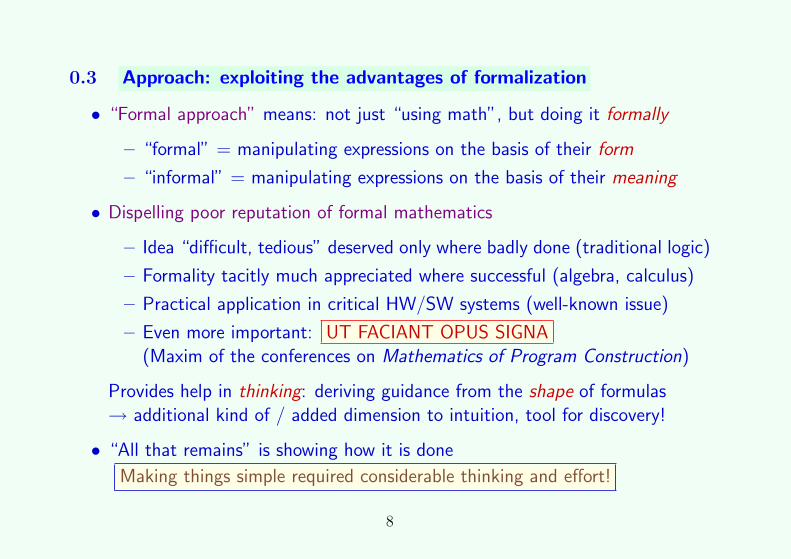
0.3 Approach: exploiting the advantages of formalization

• “Formal approach” means: not just “using math”, but doing it formally

– “formal” = manipulating expressions on the basis of their form

– “informal” = manipulating expressions on the basis of their meaning

• Dispelling poor reputation of formal mathematics

– Idea “difficult, tedious” deserved only where badly done (traditional logic)

– Formality tacitly much appreciated where successful (algebra, calculus)

– Practical application in critical HW/SW systems (well-known issue)

– Even more important: UT FACIANT OPUS SIGNA(Maxim of the conferences on Mathematics of Program Construction)

Provides help in thinking: deriving guidance from the shape of formulas→ additional kind of / added dimension to intuition, tool for discovery!

• “All that remains” is showing how it is done

Making things simple required considerable thinking and effort!

8

Next topic

09:00–09:20 0. Motivation: synergy FM-SP; value of defect-free formalismsPart I — Unifying the mathematics of SP and FM

09:20–09:40 1. Review of the basics and outline of the formalism used09:40–10:10 2. Inspiration from SP to FM: functions and functionals10:10–10:30 3. Calculation with predicates and quantifiers for engineers10:30–11:00 (Half-hour break)

Part II — Application examples to modeling in SP and FM11:00–11:40 4. Predicate calculus and generic functionals applied to classical SP11:40–11:45 5. Brief intermezzo about endosemantic functions11:45–12:05 6. Modeling programs by program equations12:05–12:25 7. Reasoning about temporal behavior by temporal operators12:25–12:30 8. Final considerations

9

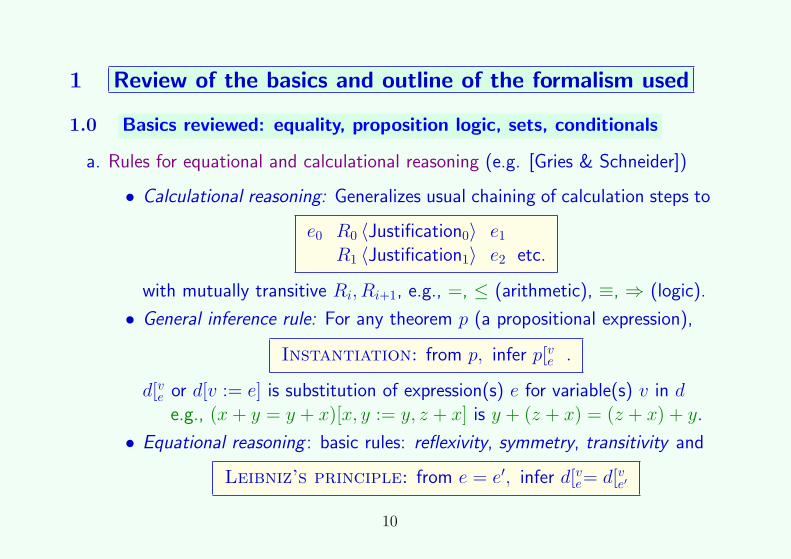
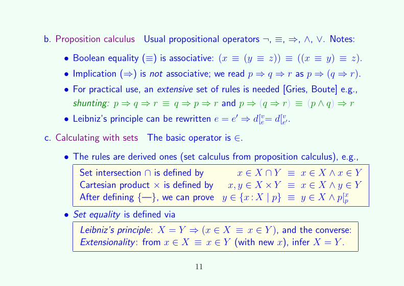
1 Review of the basics and outline of the formalism used

1.0 Basics reviewed: equality, proposition logic, sets, conditionals

a. Rules for equational and calculational reasoning (e.g. [Gries & Schneider])

• Calculational reasoning: Generalizes usual chaining of calculation steps to

e0 R0 〈Justification0〉 e1

R1 〈Justification1〉 e2 etc.

with mutually transitive Ri, Ri+1, e.g., =, ≤ (arithmetic), ≡, ⇒ (logic).

• General inference rule: For any theorem p (a propositional expression),

Instantiation: from p, infer p[ve .

d[ve or d[v := e] is substitution of expression(s) e for variable(s) v in de.g., (x+ y = y + x)[x, y := y, z + x] is y + (z + x) = (z + x) + y.

• Equational reasoning : basic rules: reflexivity, symmetry, transitivity and

Leibniz’s principle: from e = e′, infer d[ve= d[ve′

10

b. Proposition calculus Usual propositional operators ¬, ≡, ⇒, ∧, ∨. Notes:

• Boolean equality (≡) is associative: (x ≡ (y ≡ z)) ≡ ((x ≡ y) ≡ z).

• Implication (⇒) is not associative; we read p⇒ q ⇒ r as p⇒ (q ⇒ r).

• For practical use, an extensive set of rules is needed [Gries, Boute] e.g.,

shunting: p⇒ q ⇒ r ≡ q ⇒ p⇒ r and p⇒ (q ⇒ r) ≡ (p ∧ q) ⇒ r

• Leibniz’s principle can be rewritten e = e′ ⇒ d[ve= d[ve′.

c. Calculating with sets The basic operator is ∈.

• The rules are derived ones (set calculus from proposition calculus), e.g.,

Set intersection ∩ is defined by x ∈ X ∩ Y ≡ x ∈ X ∧ x ∈ YCartesian product × is defined by x, y ∈ X ×Y ≡ x ∈ X ∧ y ∈ YAfter defining {—}, we can prove y ∈ {x :X | p} ≡ y ∈ X ∧ p[xp

• Set equality is defined via

Leibniz’s principle: X = Y ⇒ (x ∈ X ≡ x ∈ Y ), and the converse:Extensionality : from x ∈ X ≡ x ∈ Y (with new x), infer X = Y .

11

d. Binary algebra and calculating with conditionals

• Principle: binary algebra as a restriction of minimax algebra, i.e., least up-per bound (∨) and greatest lower bound (∧) over R′ := R∪{−∞,+∞}.

Definition: a∨ b ≤ c ≡ a ≤ c ∧ b ≤ c and c ≤ a∧ b ≡ c ≤ a ∧ c ≤ b

Restriction to B illustrated by listing fi (x, y) for i : 1 .. 15 (functions B2→B).

x, y 0 1 2 3 4 5 6 7 8 9 10 11 12 13 14 15

0,0 0 1 0 1 0 1 0 1 0 1 0 1 0 1 0 10,1 0 0 1 1 0 0 1 1 0 0 1 1 0 0 1 11,0 0 0 0 0 1 1 1 1 0 0 0 0 1 1 1 11,1 0 0 0 0 0 0 0 0 1 1 1 1 1 1 1 1

B ∨− < > ≡/ ∧− ∧ ≡ 〉〉 ⇒ 〈〈 ⇐ ∨R′ < > 6= ∧ = 〉〉 ≤ 〈〈 ≥ ∨

• Conditionals c ? e′ e = (e, e′) c (“if c then e′ else e”) Properties:

• (c ? f g)x = c ? f x g x and f (c ? x y) = c ? f x f y

• c ? b b′ ≡ (c⇒ b) ∧ (¬ c⇒ b′) for boolean b, b′

• z = (c ? x y) ≡ (c⇒ z = x) ∧ (¬ c⇒ z = y)

12

1.1 Formalism design: Functional Mathematics (Funmath)

• Unifying formalism for continuous and discrete mathematics

− Formalism = language (notation) + formal rules

− Unifying concept: function (= domain + mapping)Functions as first-class objects and basis for unification

• The language (characteristics)

– No “ad hoc” patching of defects, but restart from systematic basis.

– Simple structure: 4 constructs: identifier, application, abstraction, tupling

· Synthesizing common notations, without their defects

· Synthesizing new useful forms of expression, in particular: “point-free”,e.g.: square = times ◦ duplicate versus square x = x times x

· If point-free power not used (pity∞!), the notation looks “standard”

• Formal rules (main characteristic): calculational

Warning: here come a few language technicalities — but they eliminate all defects!

13

The four constructs

Overview: 0. identifier, 1. application, 2. abstraction, 3. tupling

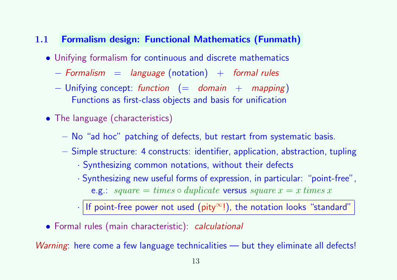
0. Identifier: any symbol or string except a (very) few keywords.

• Established symbols (e.g., B, ⇒, R, +) taken as predefined constants.

• Identifiers are introduced (or declared) by bindings

General form: i :X ∧. p , read “i in X satisfying p” (∧. p optional)

Here i is the (tuple of) identifier(s), X a set and p a proposition.

Example: n : N is interchangeable with n : Z∧. n ≥ 0

• Identifiers come in two flavors.

– Constants: declared by

· a specification of the form spec binding (no obligations)

· a definition of the form def binding (proof obligation: ∃!)

– Variables: in an abstraction binding . expression (soon!)

14

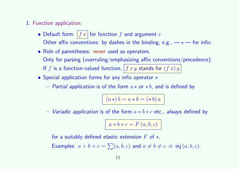
1. Function application:

• Default form: f x for function f and argument e

Other affix conventions: by dashes in the binding, e.g., — ?— for infix.

• Role of parentheses: never used as operators.

Only for parsing (overruling/emphasizing affix conventions/precedence).

If f is a function-valued function, f x y stands for (f x) y

• Special application forms for any infix operator ?

– Partial application is of the form a ? or ? b, and is defined by

(a ?) b = a ? b = (? b) a

– Variadic application is of the form a ∗ b ∗ c etc., always defined by

a ∗ b ∗ c = F (a, b, c)

for a suitably defined elastic extension F of ?.

Examples: a+ b+ c =∑

(a, b, c) and a 6= b 6= c ≡ inj (a, b, c).

15

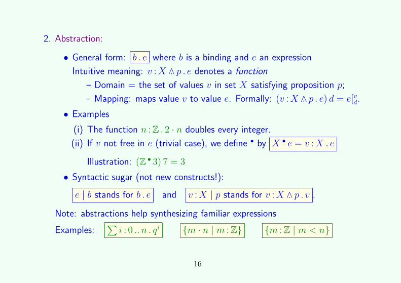
2. Abstraction:

• General form: b . e where b is a binding and e an expression

Intuitive meaning: v :X ∧. p . e denotes a function

– Domain = the set of values v in set X satisfying proposition p;

– Mapping: maps value v to value e. Formally: (v :X ∧. p . e) d = e[vd.

• Examples

(i) The function n : Z . 2 · n doubles every integer.

(ii) If v not free in e (trivial case), we define • by X • e = v :X . e

Illustration: (Z • 3) 7 = 3

• Syntactic sugar (not new constructs!):

e | b stands for b . e and v :X | p stands for v :X ∧. p . v .

Note: abstractions help synthesizing familiar expressions

Examples:∑i : 0 ..n . qi {m · n | m : Z} {m : Z | m < n}

16

3. Tupling:

• General form: e, e′, e′′ (any length) for 1 dimension

Intuitive meaning: e, e′, e′′ denotes a function

– Domain: D (e, e′, e′′) = {0, 1, 2}– Mapping: (e, e′, e′′) 0 = e and (e, e′, e′′) 1 = e′ and (e, e′, e′′) 2 = e′′.

• Parentheses are not part of tupling:

they are as optional in (m,n) as they are optional in (m+ n).

• The empty tuple is ε and for singleton tuples we define τ with τ e = 0 7→ e.

Legend: here we used two particular forms of •:

– we define ε by ε := ∅ • e (any e) for the empty function;

– we define 7→ by d 7→ e = ι d • e for one-point functions.

• Matrices are 2-dimensional tuples.

Relax! This concludes the language technicalities.

17

Next topic

09:00–09:20 0. Motivation: synergy FM-SP; value of defect-free formalismsPart I — Unifying the mathematics of SP and FM

09:20–09:40 1. Review of the basics and outline of the formalism used

09:40–10:10 2. Inspiration from SP to FM: functions and functionals

10:10–10:30 3. Calculation with predicates and quantifiers for engineers10:30–11:00 (Half-hour break)

Part II — Application examples to modeling in SP and FM11:00–11:40 4. Predicate calculus and generic functionals applied to classical SP11:40–11:45 5. Brief intermezzo about endosemantic functions11:45–12:05 6. Modeling programs by program equations12:05–12:25 7. Reasoning about temporal behavior by temporal operators12:25–12:30 8. Final considerations

18

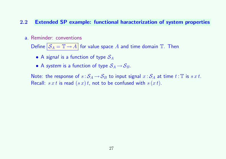
2 Inspiration from SP to FM: functions and functionals

2.0 Proper use of functions and functionals in SP: opportunities

a. Starting example: criticism of Lee & Varaiya about the common yet nonsensical

z(t) = x(t) ∗ y(t) and instantiation z(t− τ) = x(t− τ) ∗ y(t− τ)

How to do it right? Approach by L&V: see web. In the Funmath framework:

• Conventions For value space A and time domain T, define SA = T→A .

Signal : function of type SA. System: function of type SA→SB.Response of s :SA→SB to signal x :SA at time t : T is s x t, read (s x) t.

• Convolution Proper definition: for signals x and y

(x ∗ y) t =

∫ +∞

−∞x τ · y (t− τ) · dτ

Using the shift operator def σ— : T→SA→SA with στ x t = x (t+ τ)one can now express convolution of shifted signals properly as

στ x ∗ συ y = στ+υ (x ∗ y) and hence σ−τ x ∗ σ−τ y = σ−2·τ (x ∗ y)19

b. Functionals for structuring signal and system models: typical needs

• Proper formal modeling of memoryless devices for pointwise operations

– E.g., sum of signals x and y modelled as (x + y) t = x t+ y t

– Explicit direct extension operator — (in engineering often left implicit)

“Textbook” form

x

y

@@

������+ x + y LabVIEW

����

HHHH+

• Memory devices: latches (discrete case), integrators (continuous case)

Da xn = (n = 0) ? a x (n− 1) or, in point-free form, Da x = a>−x

“Textbook” form

-a>−xDa

-x

LabVIEW

5 4- - -xa a>−x

20

• Combining systems and interconnections

– The manifold role of function composition (◦)∗ Image definition: (f ◦ g)x = f (g x)

∗ Origin: cascade connection (classical)

- g - f -

∗ Other opportunity (in functional framework): system replication

-

x

- f

f

f x1

-

f x0

- f ◦x

∗ Yet another opportunity: direct extension of 1-argument operators:extension operator — with mapping g x = g ◦x

Example property: h ◦ g = h ◦ g (proof: exercise)

∗ Yet another: subsumes map from functional programming.

21

– A third operator: transposition (abeside composition, extension)

∗ Image definition: fTy x = f x y (swapping arguments)Name obviously borrowed from matrix theory

∗ (a) Origin: from a family of signals to a tuple-valued signal

∗ (b) Other opportunity: signal replication (fanout)

fs s s s s s ss s s s s s ss s s s s s s

t -

fT sss

sss

sss

sss

sss

sss

sss

(a)

-

x

- f1

f0

f1 x

-

f0 x

- fTx

(b)

∗ Other opportunity: subsumes zip from functional programming

zip[[a,b,c],[a’,b’,c’]] = [[a,a’],[b,b’],[c,c’]]

(taking lists as functions, and up to currying)

22

2.1 Formalization: calculating with functions and generic functionals

a. General rules for functions

• Equality is defined (taking domains into account) via

Leibniz: f = g ⇒ D f = D g ∧ (x ∈ D f ∩ D g ⇒ f x = g x)

Extensionality:p⇒ D f = D g ∧ (x ∈ D f ∩ D g ⇒ f x = g x)

p⇒ f = g

• Abstraction encapsulates substitution. Formal axioms:

Domain axiom: d ∈ D (v :X ∧. p . e) ≡ d ∈ X ∧ p[vdMapping axiom: d ∈ D (v :X ∧. p . e) ⇒ (v :X ∧. p . e) d = e[vd

Equality is characterized via function equality (exercise).

23

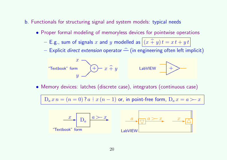
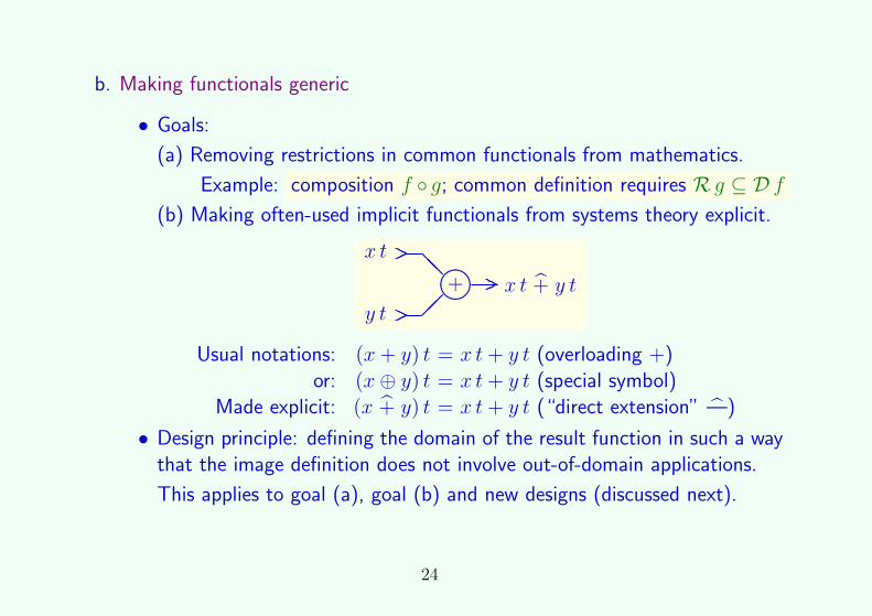
b. Making functionals generic

• Goals:

(a) Removing restrictions in common functionals from mathematics.

Example: composition f ◦ g; common definition requires R g ⊆ D f

(b) Making often-used implicit functionals from systems theory explicit.

x t

y t

@@

������+ x t + y t

Usual notations: (x+ y) t = x t+ y t (overloading +)or: (x⊕ y) t = x t+ y t (special symbol)

Made explicit: (x + y) t = x t+ y t (“direct extension” —)

• Design principle: defining the domain of the result function in such a waythat the image definition does not involve out-of-domain applications.

This applies to goal (a), goal (b) and new designs (discussed next).

24

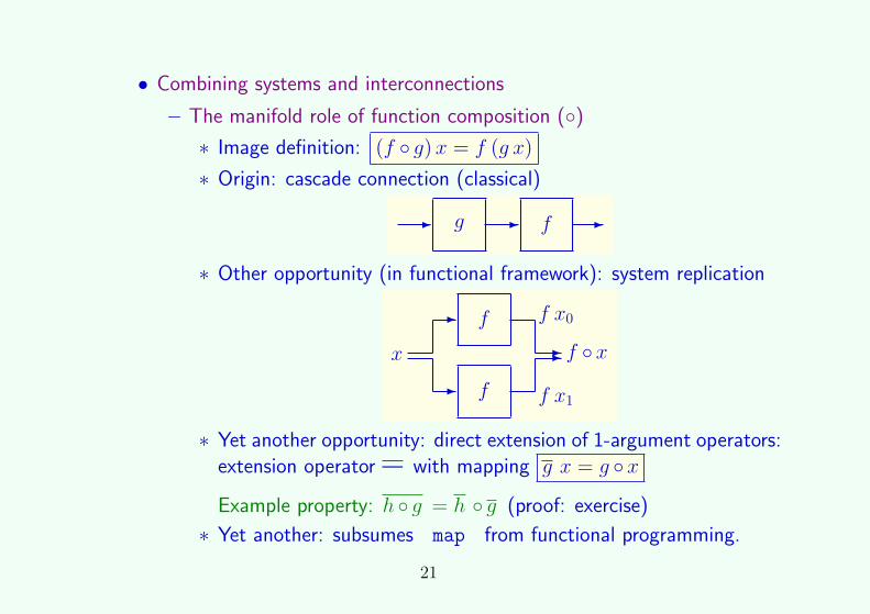
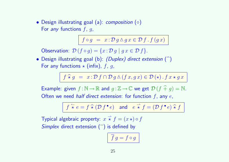
• Design illustrating goal (a): composition (◦)For any functions f , g,

f ◦ g = x :D g ∧. g x ∈ D f . f (g x)

Observation: D (f ◦ g) = {x :D g | g x ∈ D f}.• Design illustrating goal (b): (Duplex) direct extension ()

For any functions ? (infix), f , g,

f ? g = x :D f ∩ D g ∧. (f x, g x) ∈ D (?) . f x ? g x

Example: given f : N→R and g : Z→C we get D (f + g) = N.

Often we need half direct extension: for function f , any e,

f↼? e = f ? (D f • e) and e

⇀? f = (D f • e) ? f

Typical algebraic property: x⇀? f = (x ?) ◦ f

Simplex direct extension ( ) is defined by

f g = f ◦ g

25

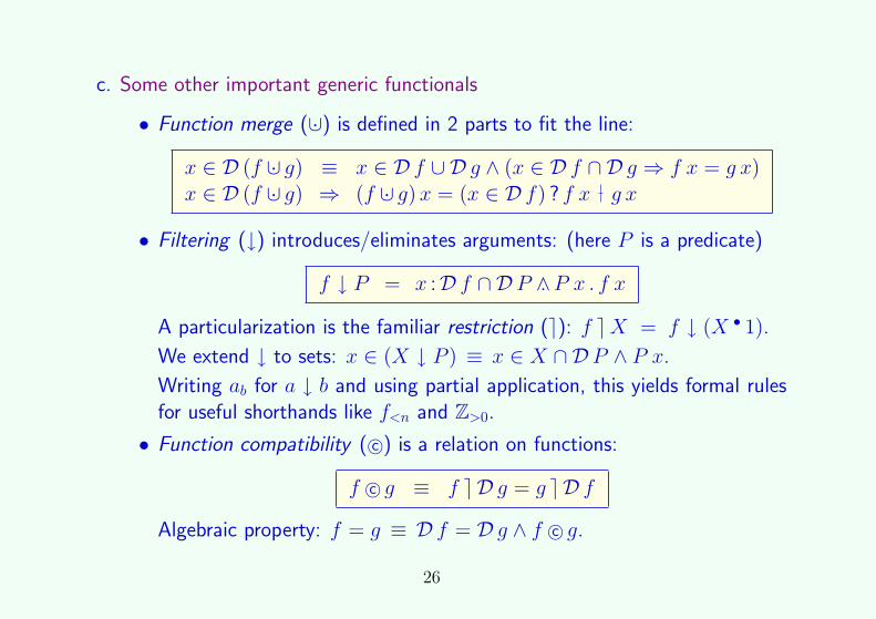
c. Some other important generic functionals

• Function merge (∪· ) is defined in 2 parts to fit the line:

x ∈ D (f ∪· g) ≡ x ∈ D f ∪ D g ∧ (x ∈ D f ∩ D g ⇒ f x = g x)x ∈ D (f ∪· g) ⇒ (f ∪· g)x = (x ∈ D f) ? f x g x

• Filtering (↓) introduces/eliminates arguments: (here P is a predicate)

f ↓ P = x :D f ∩ D P ∧. P x . f x

A particularization is the familiar restriction (e): f eX = f ↓ (X • 1).

We extend ↓ to sets: x ∈ (X ↓ P ) ≡ x ∈ X ∩ D P ∧ P x.Writing ab for a ↓ b and using partial application, this yields formal rulesfor useful shorthands like f<n and Z>0.

• Function compatibility ( c©) is a relation on functions:

f c© g ≡ f eD g = g eD f

Algebraic property: f = g ≡ D f = D g ∧ f c© g.

26

2.2 Extended SP example: functional haracterization of system properties

a. Reminder: conventions

Define SA = T→A for value space A and time domain T. Then

• A signal is a function of type SA

• A system is a function of type SA→SB.

Note: the response of s :SA→SB to input signal x :SA at time t : T is s x t.Recall: s x t is read (s x) t, not to be confused with s (x t).

27

b. Characteristics Let s :SA→SB. Then:

• System s is

memoryless iff ∃ f— : T→A→B .∀x :SA .∀ t : T . s x t = ft (x t)

• Let T be additive, and the shift function σ— be defined byστ x t = x (t+ τ) for any t and τ in T and any signal x. Then s is

time-invariant iff ∀ τ : T . s ◦στ = στ ◦ s

• Let now s :SR→SR. Then system s is linear iff∀ (x, y) :S2

R .∀ (a, b) : R2 . s (a⇀· x + b

⇀· y) = a⇀· s x + b

⇀· s y.Equivalently, extending s to SC→SC in the evident way, system s is

linear iff ∀ z :SC .∀ c : C . s (c⇀· z) = c

⇀· s z

• A system is LTI iff it is both linear and time-invariant.

28

c. Response of LTI systems

Define the parametrized exponential E— : C→T→C with Ec t = ec·t

Then we have:

Theorem: if s is LTI then sEc = sEc 0⇀· Ec

Proof: we calculate sEc (t+ τ) to exploit all properties.

sEc (t+ τ) = 〈Definition σ〉 στ (sEc) t= 〈Time inv. s〉 s (στ Ec) t

= 〈Property Ec〉 s (Ec τ⇀· Ec) t

= 〈Linearity s〉 (Ec τ⇀· sEc) t

= 〈Defintion⇀〉 Ec τ · sEc t

Substituting t := 0 yields sEc τ = sEc 0 · Ec τ or, using⇀

,sEc τ = (sEc 0

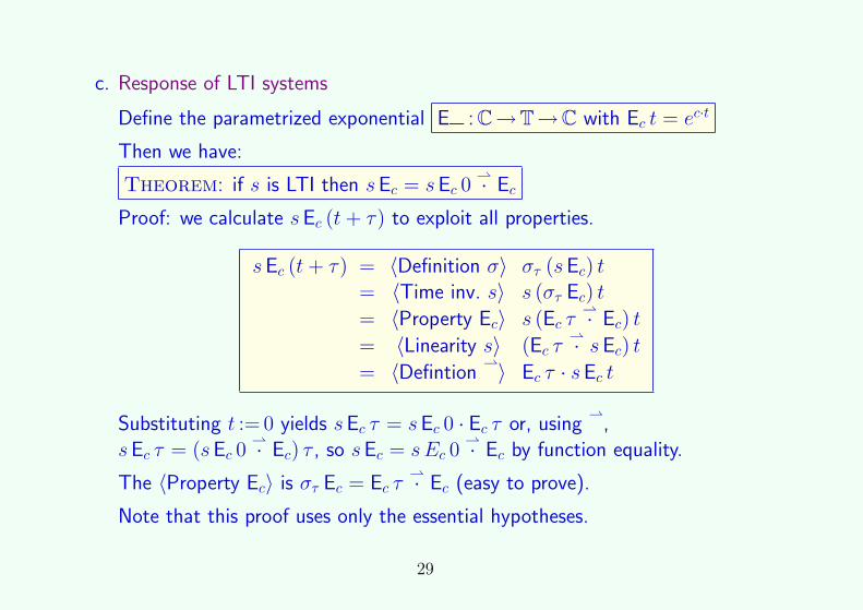
⇀· Ec) τ , so sEc = sEc 0⇀· Ec by function equality.

The 〈Property Ec〉 is στ Ec = Ec τ⇀· Ec (easy to prove).

Note that this proof uses only the essential hypotheses.

29

Next topic

09:00–09:20 0. Motivation: synergy FM-SP; value of defect-free formalismsPart I — Unifying the mathematics of SP and FM

09:20–09:40 1. Review of the basics and outline of the formalism used09:40–10:10 2. Inspiration from SP to FM: functions and functionals

10:10–10:30 3. Calculation with predicates and quantifiers for engineers

10:30–11:00 (Half-hour break)Part II — Application examples to modeling in SP and FM

11:00–11:40 4. Predicate calculus and generic functionals applied to classical SP11:40–11:45 5. Brief intermezzo about endosemantic functions11:45–12:05 6. Modeling programs by program equations12:05–12:25 7. Reasoning about temporal behavior by temporal operators12:25–12:30 8. Final considerations

30

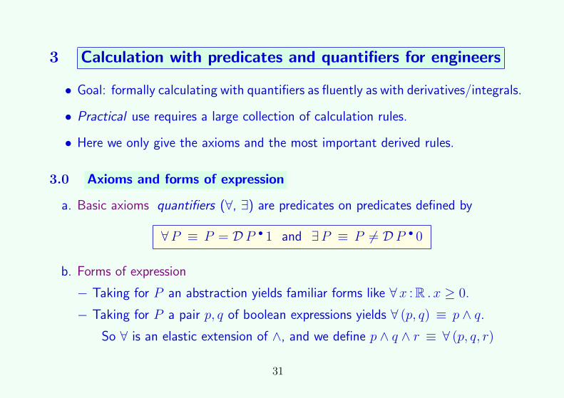
3 Calculation with predicates and quantifiers for engineers

• Goal: formally calculating with quantifiers as fluently as with derivatives/integrals.

• Practical use requires a large collection of calculation rules.

• Here we only give the axioms and the most important derived rules.

3.0 Axioms and forms of expression

a. Basic axioms quantifiers (∀, ∃) are predicates on predicates defined by

∀P ≡ P = D P • 1 and ∃P ≡ P 6= D P • 0

b. Forms of expression

− Taking for P an abstraction yields familiar forms like ∀x : R . x ≥ 0.

− Taking for P a pair p, q of boolean expressions yields ∀ (p, q) ≡ p ∧ q.So ∀ is an elastic extension of ∧, and we define p ∧ q ∧ r ≡ ∀ (p, q, r)

31

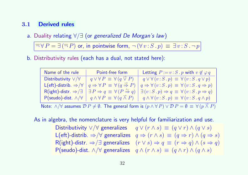
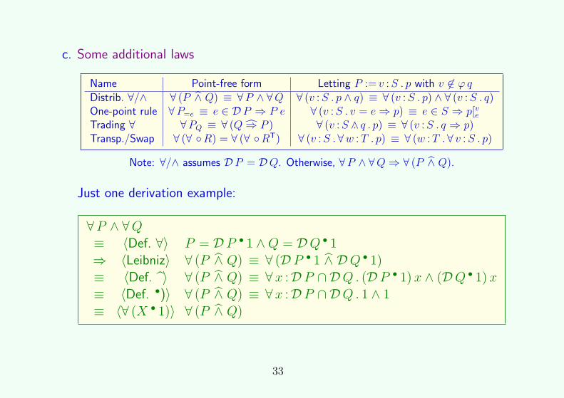
3.1 Derived rules

a. Duality relating ∀/∃ (or generalized De Morgan’s law)

¬∀P = ∃ (¬P ) or, in pointwise form, ¬ (∀ v :S . p) ≡ ∃ v :S .¬ p

b. Distributivity rules (each has a dual, not stated here):

Name of the rule Point-free form Letting P := v :S . p with v 6∈ ϕ qDistributivity ∨/∀ q ∨ ∀P ≡ ∀ (q

⇀∨ P ) q ∨ ∀ (v :S . p) ≡ ∀ (v :S . q ∨ p)L(eft)-distrib. ⇒/∀ q ⇒ ∀P ≡ ∀ (q

⇀⇒ P ) q ⇒ ∀ (v :S . p) ≡ ∀ (v :S . q ⇒ p)

R(ight)-distr. ⇒/∃ ∃P ⇒ q ≡ ∀ (P↼⇒ q) ∃ (v :S . p) ⇒ q ≡ ∀ (v :S . p⇒ q)

P(seudo)-dist. ∧/∀ q ∧ ∀P ≡ ∀ (q⇀∧ P ) q ∧ ∀ (v :S . p) ≡ ∀ (v :S . q ∧ p)

Note: ∧/∀ assumes D P 6= ∅. The general form is (p ∧ ∀P ) ∨ D P = ∅ ≡ ∀ (p⇀∧ P )

As in algebra, the nomenclature is very helpful for familiarization and use.

Distributivity ∨/∀ generalizes q ∨ (r ∧ s) ≡ (q ∨ r) ∧ (q ∨ s)L(eft)-distrib. ⇒/∀ generalizes q ⇒ (r ∧ s) ≡ (q ⇒ r) ∧ (q ⇒ s)R(ight)-distr. ⇒/∃ generalizes (r ∨ s) ⇒ q ≡ (r ⇒ q) ∧ (s⇒ q)P(seudo)-dist. ∧/∀ generalizes q ∧ (r ∧ s) ≡ (q ∧ r) ∧ (q ∧ s)

32

c. Some additional laws

Name Point-free form Letting P := v :S . p with v 6∈ ϕ qDistrib. ∀/∧ ∀ (P ∧ Q) ≡ ∀P ∧ ∀Q ∀ (v :S . p ∧ q) ≡ ∀ (v :S . p) ∧ ∀ (v :S . q)One-point rule ∀P=e ≡ e ∈ D P ⇒ P e ∀ (v :S . v = e⇒ p) ≡ e ∈ S ⇒ p[veTrading ∀ ∀PQ ≡ ∀ (Q ⇒ P ) ∀ (v :S ∧. q . p) ≡ ∀ (v :S . q ⇒ p)Transp./Swap ∀ (∀ ◦R) = ∀ (∀ ◦RT) ∀ (v :S .∀w :T . p) ≡ ∀ (w :T .∀ v :S . p)

Note: ∀/∧ assumes D P = DQ. Otherwise, ∀P ∧ ∀Q⇒ ∀ (P ∧ Q).

Just one derivation example:

∀P ∧ ∀Q≡ 〈Def. ∀〉 P = D P • 1 ∧Q = DQ • 1⇒ 〈Leibniz〉 ∀ (P ∧ Q) ≡ ∀ (D P • 1 ∧ DQ • 1)≡ 〈Def. 〉 ∀ (P ∧ Q) ≡ ∀x :D P ∩ DQ . (D P • 1)x ∧ (DQ • 1)x≡ 〈Def. •)〉 ∀ (P ∧ Q) ≡ ∀x :D P ∩ DQ . 1 ∧ 1≡ 〈∀ (X • 1)〉 ∀ (P ∧ Q)

33

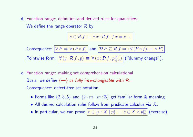
d. Function range: definition and derived rules for quantifiers

We define the range operator R by

e ∈ R f ≡ ∃x :D f . f x = e .

Consequence: ∀P ⇒ ∀ (P ◦ f) and D P ⊆ R f ⇒ (∀ (P ◦ f) ≡ ∀P )

Pointwise form: ∀ (y :R f . p) ≡ ∀ (x :D f . p[yf x) (“dummy change”).

e. Function range: making set comprehension calculational

Basis: we define {—} as fully interchangeable with R.

Consequence: defect-free set notation:

• Forms like {2, 3, 5} and {2 ·m | m : Z} get familiar form & meaning

• All desired calculation rules follow from predicate calculus via R.

• In particular, we can prove e ∈ {v :X | p} ≡ e ∈ X ∧ p[ve (exercise).

34

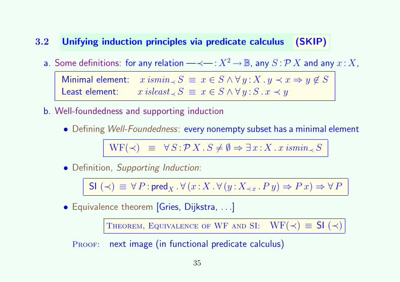
3.2 Unifying induction principles via predicate calculus (SKIP)

a. Some definitions: for any relation —≺— :X2→B, any S :P X and any x :X,

Minimal element: x ismin≺ S ≡ x ∈ S ∧ ∀ y :X . y ≺ x⇒ y 6∈ SLeast element: x isleast≺ S ≡ x ∈ S ∧ ∀ y :S . x ≺ y

b. Well-foundedness and supporting induction

• Defining Well-Foundedness: every nonempty subset has a minimal element

WF(≺) ≡ ∀S :P X .S 6= ∅ ⇒ ∃x :X . x ismin≺ S

• Definition, Supporting Induction:

SI (≺) ≡ ∀P : predX .∀ (x :X .∀ (y :X≺x . P y) ⇒ P x) ⇒ ∀P

• Equivalence theorem [Gries, Dijkstra, . . .]

Theorem, Equivalence of WF and SI: WF(≺) ≡ SI (≺)

Proof: next image (in functional predicate calculus)

35

WF(≺)≡ 〈Definition WF) and S 6= ∅ ≡ ∃x :S . 1〉∀S :P X .∃ (x :S . 1) ⇒ ∃ (x :X . x ismin≺ S)

≡ 〈S = X ∩ S, trading〉∀S :P X .∃ (x :X . x ∈ S) ⇒ ∃ (x :X . x ismin≺ S)

≡ 〈Definition ismin〉∀S :P X .∃ (x :X . x ∈ S) ⇒ ∃ (x :X . x ∈ S ∧ ∀ y :X . y ≺ x⇒ y 6∈ S)

≡ 〈p⇒ q ≡ ¬ q ⇒ ¬ p〉∀S :P X .¬ (∃x :X . x ∈ S ∧ ∀ y :X . y ≺ x⇒ y 6∈ S) ⇒ ¬ (∃x :X . x ∈ S)

≡ 〈Duality ∀/∃, De Morgan〉∀S :P X .∀ (x :X . x 6∈ S ∨ ¬ (∀ y :X . y ≺ x⇒ y 6∈ S)) ⇒ ∀x :X . x 6∈ S

≡ 〈∨ to ⇒, i.e., a ∨ ¬ b ≡ b⇒ a〉∀S :P X .∀ (x :X .∀ (y :X . y ≺ x⇒ y 6∈ S) ⇒ x 6∈ S) ⇒ ∀x :X . x 6∈ S

≡ 〈Dummy change using f : predX →P X with x ∈ f x ≡ ¬ (P x)〉∀P :X→B .∀ (x :X .∀ (y :X . y ≺ x⇒ P y) ⇒ P x) ⇒ ∀x :X .P x

≡ 〈Trading, definition SI 〉SI (≺)

36

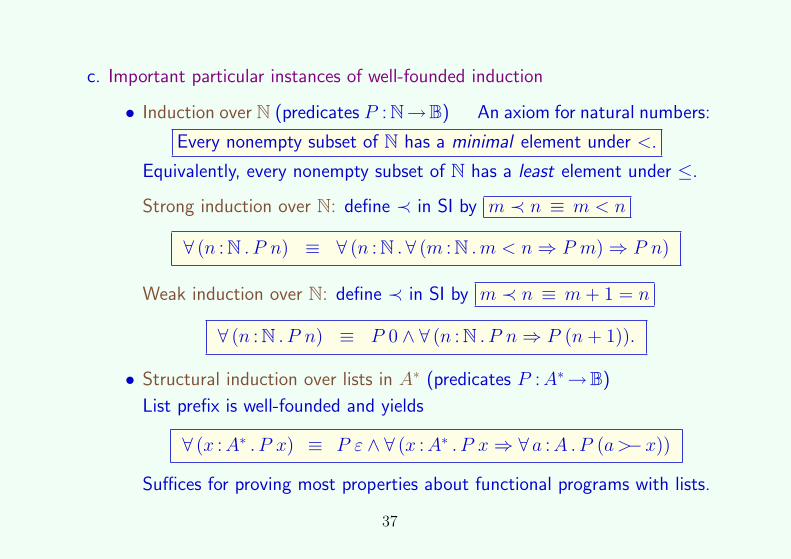
c. Important particular instances of well-founded induction

• Induction over N (predicates P : N→B) An axiom for natural numbers:

Every nonempty subset of N has a minimal element under <.

Equivalently, every nonempty subset of N has a least element under ≤.

Strong induction over N: define ≺ in SI by m ≺ n ≡ m < n

∀ (n : N . P n) ≡ ∀ (n : N .∀ (m : N .m < n⇒ P m) ⇒ P n)

Weak induction over N: define ≺ in SI by m ≺ n ≡ m+ 1 = n

∀ (n : N . P n) ≡ P 0 ∧ ∀ (n : N . P n⇒ P (n+ 1)).

• Structural induction over lists in A∗ (predicates P :A∗→B)

List prefix is well-founded and yields

∀ (x :A∗ . P x) ≡ P ε ∧ ∀ (x :A∗ . P x⇒ ∀ a :A .P (a>−x))

Suffices for proving most properties about functional programs with lists.

37

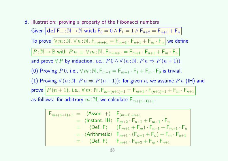
d. Illustration: proving a property of the Fibonacci numbers

Given def F— : N→N with F0 = 0 ∧ F1 = 1 ∧ Fn+2 = Fn+1 + Fn

To prove ∀m : N .∀n : N .Fm+n+1 = Fm+1 · Fn+1 + Fm · Fn we define

P : N→B with P n ≡ ∀m : N .Fm+n+1 = Fm+1 · Fn+1 + Fm · Fn

and prove ∀P by induction, i.e., P 0 ∧ ∀ (n : N . P n⇒ P (n+ 1)).

(0) Proving P 0, i.e., ∀m : N .Fm+1 = Fm+1 · F1 + Fm · F0 is trivial.

(1) Proving ∀ (n : N . P n⇒ P (n+ 1)): for given n, we assume P n (IH) and

prove P (n+ 1), i.e., ∀m : N .Fm+(n+1)+1 = Fm+1 · F(n+1)+1 + Fm · Fn+1

as follows: for arbitrary m : N, we calculate Fm+(n+1)+1.

Fm+(n+1)+1 = 〈Assoc. +〉 F(m+1)+n+1

= 〈Instant. IH〉 Fm+2 · Fn+1 + Fm+1 · Fn

= 〈Def. F〉 (Fm+1 + Fm) · Fn+1 + Fm+1 · Fn

= 〈Arithmetic〉 Fm+1 · (Fn+1 + Fn) + Fm · Fn+1

= 〈Def. F〉 Fm+1 · Fn+2 + Fm · Fn+1

38

Next topic

09:00–09:20 0. Motivation: synergy FM-SP; value of defect-free formalismsPart I — Unifying the mathematics of SP and FM

09:20–09:40 1. Review of the basics and outline of the formalism used09:40–10:10 2. Inspiration from SP to FM: functions and functionals10:10–10:30 3. Calculation with predicates and quantifiers for engineers10:30–11:00 (Half-hour break)

Part II — Application examples to modeling in SP and FM

11:00–11:40 4. Predicate calculus and generic functionals applied to classical SP

11:40–11:45 5. Brief intermezzo about endosemantic functions11:45–12:05 6. Modeling programs by program equations12:05–12:25 7. Reasoning about temporal behavior by temporal operators12:25–12:30 8. Final considerations

39

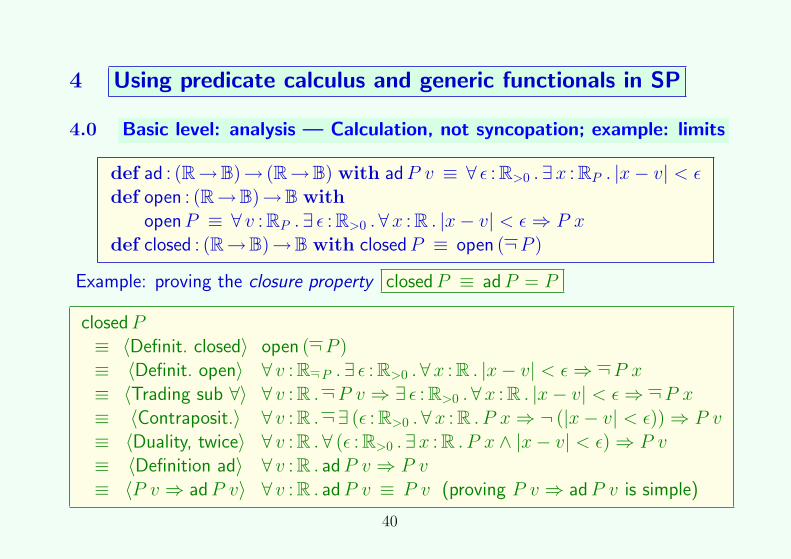
4 Using predicate calculus and generic functionals in SP

4.0 Basic level: analysis — Calculation, not syncopation; example: limits

def ad : (R→B)→ (R→B) with adP v ≡ ∀ ε : R>0 .∃x : RP . |x− v| < ε

def open : (R→B)→B withopenP ≡ ∀ v : RP .∃ ε : R>0 .∀x : R . |x− v| < ε⇒ P x

def closed : (R→B)→B with closedP ≡ open (¬P )

Example: proving the closure property closedP ≡ adP = P

closedP≡ 〈Definit. closed〉 open (¬P )≡ 〈Definit. open〉 ∀ v : R¬P .∃ ε : R>0 .∀x : R . |x− v| < ε⇒ ¬P x≡ 〈Trading sub ∀〉 ∀ v : R .¬P v ⇒ ∃ ε : R>0 .∀x : R . |x− v| < ε⇒ ¬P x≡ 〈Contraposit.〉 ∀ v : R .¬∃ (ε : R>0 .∀x : R . P x⇒ ¬ (|x− v| < ε)) ⇒ P v

≡ 〈Duality, twice〉 ∀ v : R .∀ (ε : R>0 .∃x : R . P x ∧ |x− v| < ε) ⇒ P v

≡ 〈Definition ad〉 ∀ v : R . adP v ⇒ P v

≡ 〈P v ⇒ adP v〉 ∀ v : R . adP v ≡ P v (proving P v ⇒ adP v is simple)

40

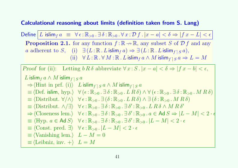
Calculational reasoning about limits (definition taken from S. Lang)

Define L islimf a ≡ ∀ ε : R>0 .∃ δ : R>0 .∀x :D f . |x− a| < δ ⇒ |f x− L| < ε

Proposition 2.1. for any function f : R→/ R, any subset S of D f and anya adherent to S, (i) ∃ (L : R . L islimf a) ⇒ ∃ (L : R . L islimf eS a),

(ii) ∀L : R .∀M : R . L islimf a ∧M islimf eS a⇒ L = M

Proof for (ii): Letting bR δ abbreviate ∀x :S . |x− a| < δ ⇒ |f x− b| < ε,

L islimf a ∧M islimf eS a

⇒〈Hint in prf. (i)〉 L islimf eS a ∧M islimf eS a

≡〈Def. islim, hyp.〉 ∀ (ε : R>0 .∃ δ : R>0 . LR δ) ∧ ∀ (ε : R>0 .∃ δ : R>0 .M R δ)≡ 〈Distribut. ∀/∧〉 ∀ ε : R>0 .∃ (δ : R>0 . LR δ) ∧ ∃ (δ : R>0 .M R δ)≡ 〈Distribut. ∧/∃〉 ∀ ε : R>0 .∃ δ : R>0 .∃ δ′ : R>0 . LR δ ∧M Rδ′

⇒〈Closeness lem.〉 ∀ ε : R>0 .∃ δ : R>0 .∃ δ′ : R>0 . a ∈ AdS ⇒ |L−M | < 2 · ε≡ 〈Hyp. a ∈ AdS〉 ∀ ε : R>0 .∃ δ : R>0 .∃ δ′ : R>0 . |L−M | < 2 · ε≡ 〈Const. pred. ∃〉 ∀ ε : R>0 . |L−M | < 2 · ε≡ 〈Vanishing lem.〉 L−M = 0≡〈Leibniz, inv. +〉 L = M

41

4.1 At the functional level in SP: transforms as functionals

a. The Fourier transform as a functional Note: not F {f(t)} but F f ω

F f ω =

∫ +∞

−∞e−j·ω·t · f t · dt and F ′g t =

1

2 · π·∫ +∞

−∞ej·ω·t · g ω · dω

Clear and unambiguous bindings allow formal calculation.

b. Functional Laplace transform via Fourier transform.

Conditioning function: `— : R→R→R with `σ t = (t < 0) ? 0 e−σ·t

We define the Laplace-transform L f of a function f by:

L f (σ + j · ω) = F (`σ · f)ω

for real σ and ω, with σ such that `σ · f has a Fourier transform.

With s :=σ + j · ω we obtain (exercise)

L f s =

∫ +∞

0f t · e−s·t · dt

42

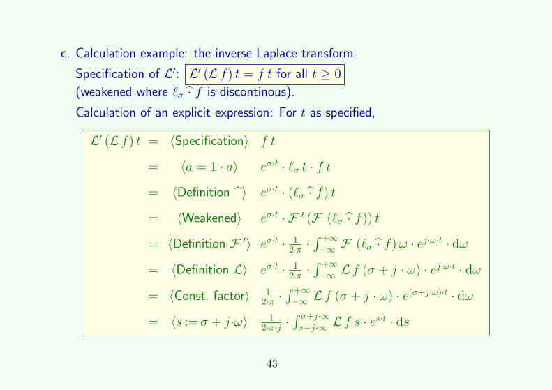
c. Calculation example: the inverse Laplace transform

Specification of L′: L′ (L f) t = f t for all t ≥ 0

(weakened where `σ · f is discontinous).

Calculation of an explicit expression: For t as specified,

L′ (L f) t = 〈Specification〉 f t

= 〈a = 1 · a〉 eσ·t · `σ t · f t

= 〈Definition 〉 eσ·t · (`σ · f) t

= 〈Weakened〉 eσ·t · F ′ (F (`σ · f)) t

= 〈Definition F ′〉 eσ·t · 12·π ·

∫ +∞−∞ F (`σ · f)ω · ej·ω·t · dω

= 〈Definition L〉 eσ·t · 12·π ·

∫ +∞−∞ L f (σ + j · ω) · ej·ω·t · dω

= 〈Const. factor〉 12·π ·

∫ +∞−∞ L f (σ + j · ω) · e(σ+j·ω)·t · dω

= 〈s :=σ + j·ω〉 12·π·j ·

∫ σ+j·∞σ−j·∞ L f s · es·t · ds

43

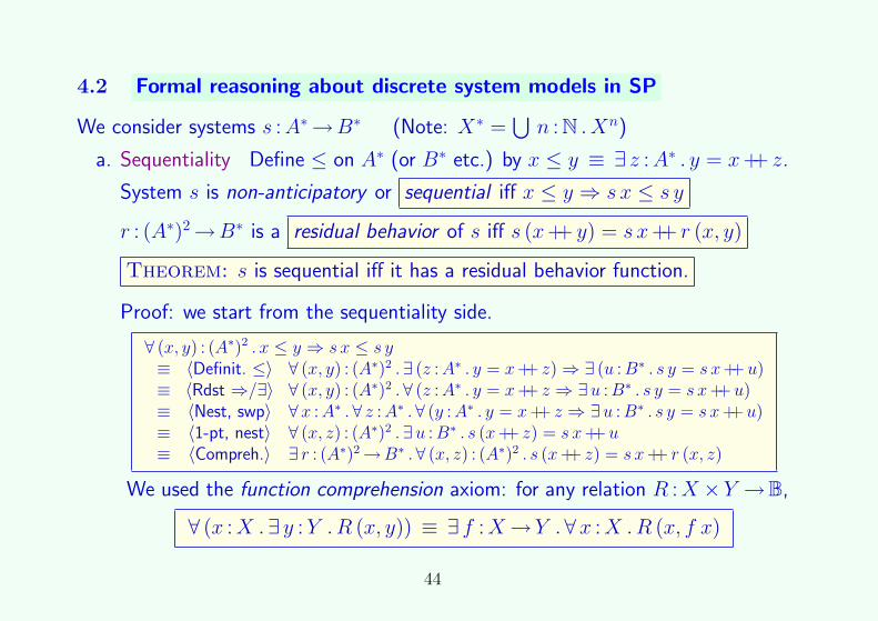
4.2 Formal reasoning about discrete system models in SP

We consider systems s :A∗→B∗ (Note: X∗ =⋃n : N . Xn)

a. Sequentiality Define ≤ on A∗ (or B∗ etc.) by x ≤ y ≡ ∃ z :A∗ . y = x++ z.

System s is non-anticipatory or sequential iff x ≤ y ⇒ s x ≤ s y

r : (A∗)2→B∗ is a residual behavior of s iff s (x++ y) = s x++ r (x, y)

Theorem: s is sequential iff it has a residual behavior function.

Proof: we start from the sequentiality side.

∀ (x, y) : (A∗)2 . x ≤ y ⇒ s x ≤ s y≡ 〈Definit. ≤〉 ∀ (x, y) : (A∗)2 .∃ (z :A∗ . y = x++ z) ⇒ ∃ (u :B∗ . s y = s x++u)≡ 〈Rdst ⇒/∃〉 ∀ (x, y) : (A∗)2 .∀ (z :A∗ . y = x++ z ⇒ ∃u :B∗ . s y = s x++u)≡ 〈Nest, swp〉 ∀x :A∗ .∀ z :A∗ .∀ (y :A∗ . y = x++ z ⇒ ∃u :B∗ . s y = s x++u)≡ 〈1-pt, nest〉 ∀ (x, z) : (A∗)2 .∃u :B∗ . s (x++ z) = s x++u≡ 〈Compreh.〉 ∃ r : (A∗)2→B∗ .∀ (x, z) : (A∗)2 . s (x++ z) = s x++ r (x, z)

We used the function comprehension axiom: for any relation R :X ×Y →B,

∀ (x :X .∃ y :Y .R (x, y)) ≡ ∃ f :X→Y . ∀x :X .R (x, f x)

44

b. Derivatives and primitives The preceding framework leads to the following.

• Observation: An rb function is unique (exercise).

• We define the derivation operator D on sequential systems by

D s ε = ε and D s (x−<a) = s x++ D s (x−<a)

With the rb function r of s, D s (x−<a) = r (x, τ a).

• Primitivation I is defined for any g :A∗→B∗ by

I g ε = ε and I g (x−<a) = I g x++ g (x++ a)

• Properties (note a striking analogy from analysis)

s (x−<a) = s x++ D s (x−<a) s x = s ε++ I (D s)xf (x+ h) ≈ f x+ D f x · h f x = f 0 + I (D f)x

In the second row, D is derivation as in analysis, and I g x =∫ x

0 g y · d y.

• The state space is {y :A∗ . r (x, y) | x :A∗} .

45

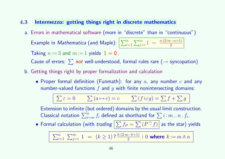
4.3 Intermezzo: getting things right in discrete mathematics

a. Errors in mathematical software (more in “discrete” than in “continuous”)

Example in Mathematica (and Maple):∑n

i=1∑m

j=i 1 = n·(2·m−n+1)2

Taking n := 3 and m := 1 yields 1 = 0 .

Cause of errors:∑

not well-understood, formal rules rare (→ syncopation)

b. Getting things right by proper formalization and calculation

• Proper formal definition (Funmath): for any a, any number c and anynumber-valued functions f and g with finite nonintersecting domains:∑

ε = 0∑

(a 7→ c) = c∑

(f ∪· g) =∑f +

∑g

Extension to infinite (but ordered) domains by the usual limit construction.Classical notation

∑ni=m fi defined as shorthand for

∑i :m ..n . fi.

• Formal calculation (with trading∑fP =

∑(P · f) as the star) yields∑n

i=1∑m

j=i 1 = (k ≥ 1) ? k·(2·m−k+1)2 0 where k :=m∧n

46

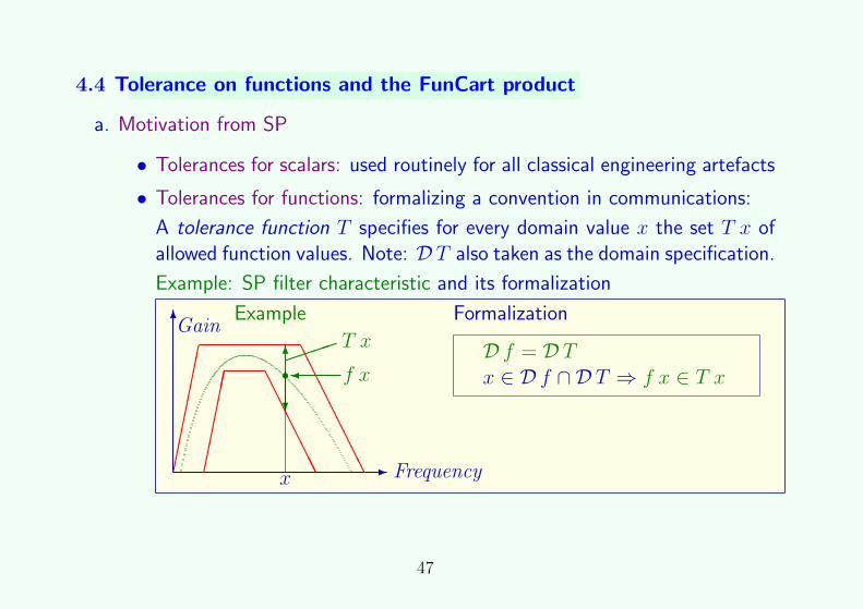
4.4 Tolerance on functions and the FunCart product

a. Motivation from SP

• Tolerances for scalars: used routinely for all classical engineering artefacts

• Tolerances for functions: formalizing a convention in communications:

A tolerance function T specifies for every domain value x the set T x ofallowed function values. Note: D T also taken as the domain specification.

Example: SP filter characteristic and its formalization

6

-

Gain

Frequency��������� A

AAAAAAAA�

������� A

AAAAAAA

6

?

���� T x

� f xs

x

Example Formalization

D f = D T

x ∈ D f ∩ D T ⇒ f x ∈ T x

47

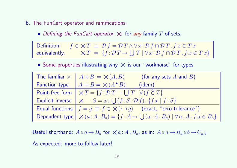
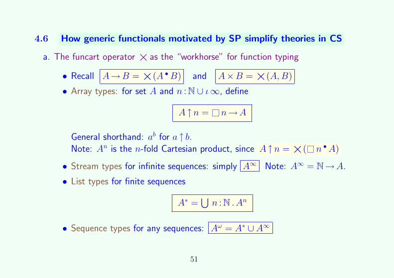
b. The FunCart operator and ramifications

• Defining the FunCart operator ×: for any family T of sets,

Definition: f ∈×T ≡ D f = D T ∧ ∀x :D f ∩ D T . f x ∈ T xequivalently, ×T = {f :D T →

⋃T | ∀x :D f ∩ D T . f x ∈ T x}

• Some properties illustrating why × is our “workhorse” for types

The familiar × A×B =×(A,B) (for any sets A and B)

Function type A→B =×(A •B) (idem)

Point-free form ×T = {f :D T →⋃T | ∀ (f ∈ T}

Explicit inverse ×− S = x :⋃

(f :S .D f) . {f x | f :S}Equal functions f = g ≡ f ∈×(ι ◦ g) (exact, “zero tolerance”)

Dependent type ×(a :A .Ba) = {f :A→⋃

(a :A .Ba) | ∀ a :A . f a ∈ Ba}

Useful shorthand: A 3 a→Ba for ×a :A .Ba, as in: A 3 a→Ba 3 b→Ca,b

As expected: more to follow later!

48

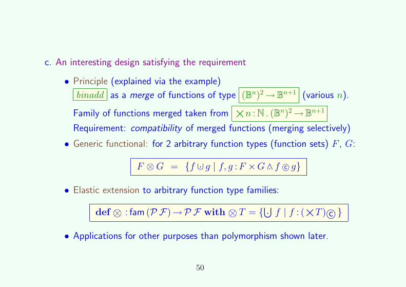
4.5 Generic functionals for overloading and polymorphism (SKIP)

a. Terminology (0) and main issues (1)

(0) Overloading: same identifier designating “different” objects (functions).Polymorphism: different argument types, formally same image definition.

(1) Disambiguation: via argument type. Means: compatibility ( c©)Refined typing: link argument/result type. Means: proper operator

b. Kinds of overloading/polymorphism

• By explicit parametrization Trivial with ×.Example: binary addition function adding two binary words of equal length.

def binadd— :×n : N . (Bn)2→Bn+1 with binaddn (x, y) = . . .

• Without auxiliary parameter (to be designed next)

Requirement: operator ⊗ with properties exemplified for binadd by

def binadd :⊗n : N . (Bn)2→Bn+1 with binadd (x, y) = . . .

49

c. An interesting design satisfying the requirement

• Principle (explained via the example)

binadd as a merge of functions of type (Bn)2→Bn+1 (various n).

Family of functions merged taken from ×n : N . (Bn)2→Bn+1

Requirement: compatibility of merged functions (merging selectively)

• Generic functional: for 2 arbitrary function types (function sets) F , G:

F ⊗G = {f ∪· g | f, g :F ×G∧. f c© g}

• Elastic extension to arbitrary function type families:

def⊗ : fam (P F)→P F with⊗T = {⋃· f | f : (×T ) c©}

• Applications for other purposes than polymorphism shown later.

50

4.6 How generic functionals motivated by SP simplify theories in CS

a. The funcart operator ×as the “workhorse” for function typing

• Recall A→B =×(A •B) and A×B =×(A,B)

• Array types: for set A and n : N ∪ ι∞, define

A ↑n = n→A

General shorthand: ab for a ↑ b.Note: An is the n-fold Cartesian product, since A ↑n =×( n •A)

• Stream types for infinite sequences: simply A∞ Note: A∞ = N→A.

• List types for finite sequences

A∗ =⋃n : N . An

• Sequence types for any sequences: Aω = A∗ ∪ A∞

51

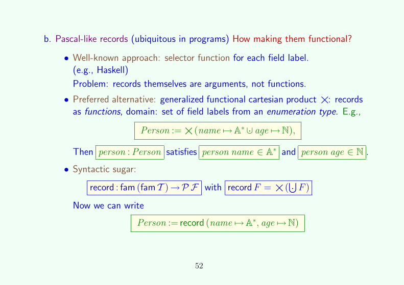
b. Pascal-like records (ubiquitous in programs) How making them functional?

• Well-known approach: selector function for each field label.(e.g., Haskell)

Problem: records themselves are arguments, not functions.

• Preferred alternative: generalized functional cartesian product×: recordsas functions, domain: set of field labels from an enumeration type. E.g.,

Person :=×(name 7→A∗ ∪· age 7→N),

Then person :Person satisfies person name ∈ A∗ and person age ∈ N .

• Syntactic sugar:

record : fam (fam T )→P F with recordF =×(⋃· F )

Now we can write

Person := record (name 7→A∗, age 7→N)

52

c. Relational databases in functional style

Database system = storing information + convenient user interfacePresentation: offering precisely the information wanted as “virtual tables”.

Code Name Instructor Prerequisites

CS100 Basic Mathematics for CS R. Barns noneMA115 Introduction to Probability K. Jason MA100CS300 Formal Methods in Engineering R. Barns CS100, EE150· · · · · · · · ·

Relational database presents the tables as relations.

• Traditional view: rows as tuples (and tuples not seen as functions).Problem: access only by separate indexing function using numbers.Patch: “grafting” attribute names for column headings.Disadvantages: model not purely relational, operators on tables ad hoc.

• Functional view; the table rows as records using recordF =×(⋃· F )

Advantage: embedding in general framework, inheriting algebraic propertiesand generic operators, record field labels supply table headings.

53

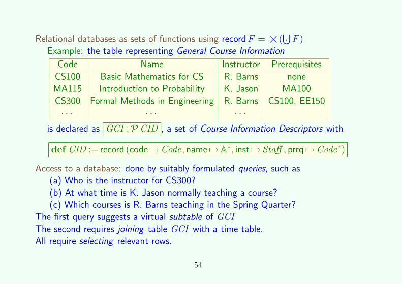
Relational databases as sets of functions using recordF =×(⋃· F )

Example: the table representing General Course Information

Code Name Instructor Prerequisites

CS100 Basic Mathematics for CS R. Barns noneMA115 Introduction to Probability K. Jason MA100CS300 Formal Methods in Engineering R. Barns CS100, EE150· · · · · · · · ·

is declared as GCI :P CID , a set of Course Information Descriptors with

def CID := record (code 7→Code, name 7→A∗, inst 7→ Staff , prrq 7→Code∗)

Access to a database: done by suitably formulated queries, such as(a) Who is the instructor for CS300?(b) At what time is K. Jason normally teaching a course?(c) Which courses is R. Barns teaching in the Spring Quarter?

The first query suggests a virtual subtable of GCIThe second requires joining table GCI with a time table.All require selecting relevant rows.

54

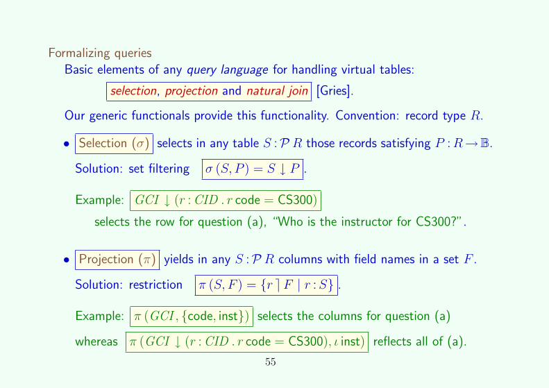
Formalizing queriesBasic elements of any query language for handling virtual tables:

selection, projection and natural join [Gries].

Our generic functionals provide this functionality. Convention: record type R.

• Selection (σ) selects in any table S :P R those records satisfying P :R→B.

Solution: set filtering σ (S, P ) = S ↓ P .

Example: GCI ↓ (r :CID . r code = CS300)

selects the row for question (a), “Who is the instructor for CS300?”.

• Projection (π) yields in any S :P R columns with field names in a set F .

Solution: restriction π (S, F ) = {r eF | r :S} .

Example: π (GCI , {code, inst}) selects the columns for question (a)

whereas π (GCI ↓ (r :CID . r code = CS300), ι inst) reflects all of (a).

55

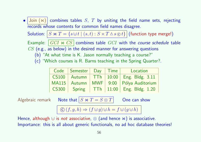
• Join (on) combines tables S, T by uniting the field name sets, rejectingrecords whose contents for common field names disagree.

Solution: S on T = {s∪· t | (s, t) : S×T ∧. s c© t} (function type merge!)

Example: GCI on CS combines table GCI with the course schedule tableCS (e.g., as below) in the desired manner for answering questions

(b) “At what time is K. Jason normally teaching a course?”(c) “Which courses is R. Barns teaching in the Spring Quarter?.

Code Semester Day Time Location

CS100 Autumn TTh 10:00 Eng. Bldg. 3.11MA115 Autumn MWF 9:00 Polya AuditoriumCS300 Spring TTh 11:00 Eng. Bldg. 1.20

Algebraic remark Note that S on T = S ⊗ T One can show

c© (f, g, h) ⇒ (f ∪· g)∪· h = f ∪· (g ∪· h)

Hence, although ∪· is not associative, ⊗ (and hence on) is associative.Importance: this is all about generic functionals, no ad hoc database theories!

56

Next topic

09:00–09:20 0. Motivation: synergy FM-SP; value of defect-free formalismsPart I — Unifying the mathematics of SP and FM

09:20–09:40 1. Review of the basics and outline of the formalism used09:40–10:10 2. Inspiration from SP to FM: functions and functionals10:10–10:30 3. Calculation with predicates and quantifiers for engineers10:30–11:00 (Half-hour break)

Part II — Application examples to modeling in SP and FM11:00–11:40 4. Predicate calculus and generic functionals applied to classical SP

11:40–11:45 5. Brief intermezzo about endosemantic functions11:45–12:05 6. Modeling programs by program equations12:05–12:25 7. Reasoning about temporal behavior by temporal operators12:25–12:30 8. Final considerations

57

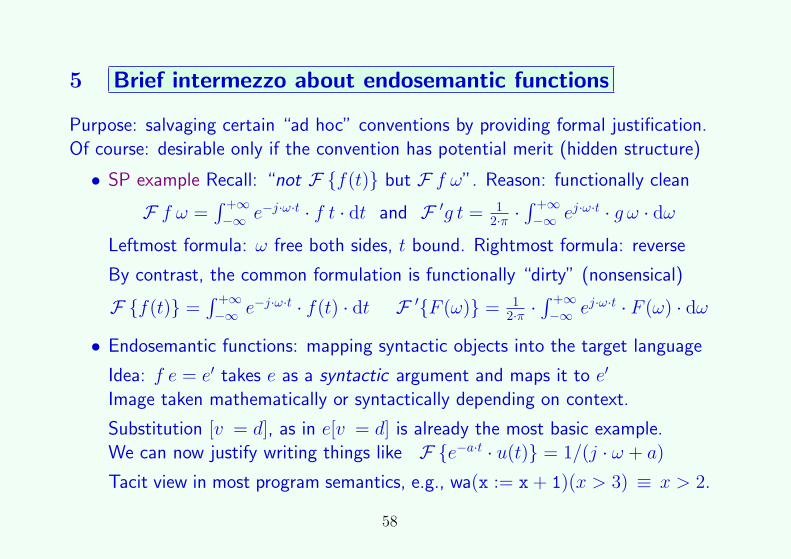
5 Brief intermezzo about endosemantic functions

Purpose: salvaging certain “ad hoc” conventions by providing formal justification.Of course: desirable only if the convention has potential merit (hidden structure)

• SP example Recall: “not F {f(t)} but F f ω”. Reason: functionally clean

F f ω =∫ +∞−∞ e−j·ω·t · f t · dt and F ′g t = 1

2·π ·∫ +∞−∞ ej·ω·t · g ω · dω

Leftmost formula: ω free both sides, t bound. Rightmost formula: reverse

By contrast, the common formulation is functionally “dirty” (nonsensical)

F {f(t)} =∫ +∞−∞ e−j·ω·t · f(t) · dt F ′{F (ω)} = 1

2·π ·∫ +∞−∞ ej·ω·t · F (ω) · dω

• Endosemantic functions: mapping syntactic objects into the target language

Idea: f e = e′ takes e as a syntactic argument and maps it to e′

Image taken mathematically or syntactically depending on context.

Substitution [v = d], as in e[v = d] is already the most basic example.We can now justify writing things like F {e−a·t · u(t)} = 1/(j · ω + a)

Tacit view in most program semantics, e.g., wa(x := x + 1)(x > 3) ≡ x > 2.

58

Next topic

09:00–09:20 0. Motivation: synergy FM-SP; value of defect-free formalismsPart I — Unifying the mathematics of SP and FM

09:20–09:40 1. Review of the basics and outline of the formalism used09:40–10:10 2. Inspiration from SP to FM: functions and functionals10:10–10:30 3. Calculation with predicates and quantifiers for engineers10:30–11:00 (Half-hour break)

Part II — Application examples to modeling in SP and FM11:00–11:40 4. Predicate calculus and generic functionals applied to classical SP11:40–11:45 5. Brief intermezzo about endosemantic functions

11:45–12:05 6. Modeling programs by program equations

12:05–12:25 7. Reasoning about temporal behavior by temporal operators12:25–12:30 8. Final considerations

59

6 Modeling programs by program equations

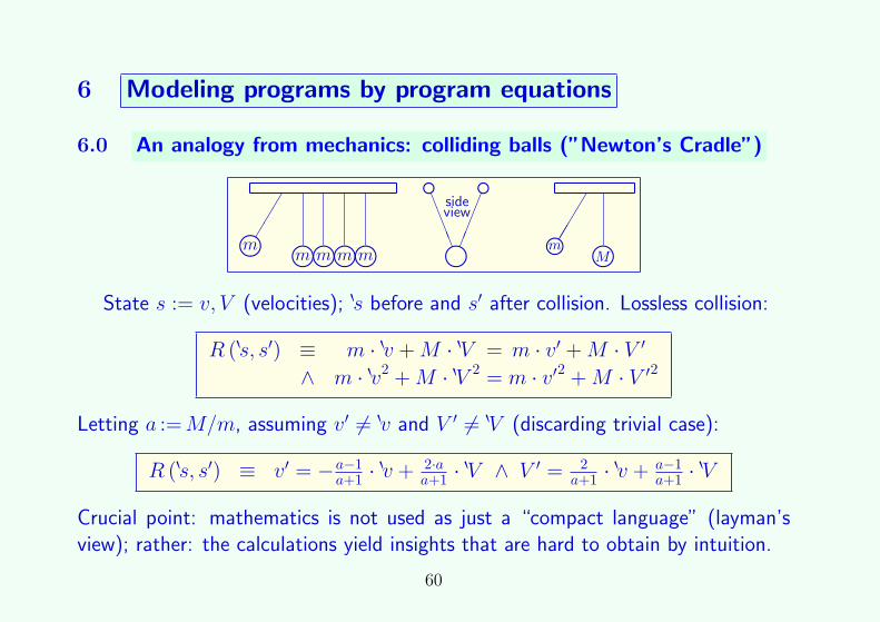
6.0 An analogy from mechanics: colliding balls (”Newton’s Cradle”)

mm�

�� mm mm mm mm

f fm

LLLL

��

��

sideview jm mM

��

��

State s := v, V (velocities); 8s before and s′ after collision. Lossless collision:

R (8s, s′) ≡ m · 8v +M · 8V = m · v′ +M · V ′

∧ m · 8v2 +M · 8V 2 = m · v′2 +M · V ′2

Letting a :=M/m, assuming v′ 6= 8v and V ′ 6= 8V (discarding trivial case):

R (8s, s′) ≡ v′ = −a−1a+1 ·

8v + 2·aa+1 ·

8V ∧ V ′ = 2a+1 ·

8v + a−1a+1 ·

8V

Crucial point: mathematics is not used as just a “compact language” (layman’sview); rather: the calculations yield insights that are hard to obtain by intuition.

60

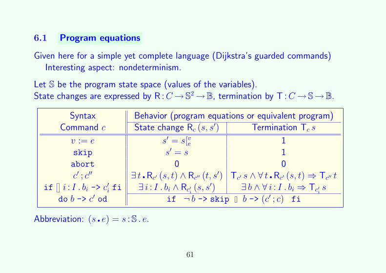
6.1 Program equations

Given here for a simple yet complete language (Dijkstra’s guarded commands)Interesting aspect: nondeterminism.

Let S be the program state space (values of the variables).State changes are expressed by R :C→S2→B, termination by T :C→S→B.

Syntax Behavior (program equations or equivalent program)Command c State change Rc (s, s′) Termination Tc s

v := e s′ = s[ve 1skip s′ = s 1abort 0 0c′ ; c′′ ∃ t • Rc′ (s, t) ∧ Rc′′ (t, s

′) Tc′ s ∧ ∀ t • Rc′ (s, t) ⇒ Tc′′ t

if i : I . bi -> c′i fi ∃ i : I . bi ∧ Rc′i

(s, s′) ∃ b ∧ ∀ i : I . bi ⇒ Tc′is

do b -> c′ od if ¬ b -> skip b -> (c′ ; c) fi

Abbreviation: (s • e) = s : S . e.

61

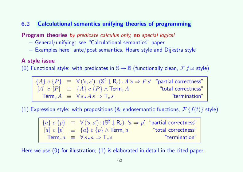
6.2 Calculational semantics unifying theories of programming

Program theories by predicate calculus only, no special logics!− General/unifying: see “Calculational semantics” paper− Examples here: ante/post semantics, Hoare style and Dijkstra style

A style issue(0) Functional style: with predicates in S→B (functionally clean, F f ω style)

{A} c {P} ≡ ∀ (8s, s′) : (S2 ↓ Rc) . A8s⇒ P s′ “partial correctness”

[A] c [P ] ≡ {A} c {P} ∧ TermcA “total correctness”TermcA ≡ ∀ s •As⇒ Tc s “termination”

(1) Expression style: with propositions (& endosemantic functions, F {f(t)} style)

{a} c {p} ≡ ∀ (8s, s′) : (S2 ↓ Rc) .8a⇒ p′ “partial correctness”

[a] c [p] ≡ {a} c {p} ∧ Termc a “total correctness”Termc a ≡ ∀ s • a⇒ Tc s “termination”

Here we use (0) for illustration; (1) is elaborated in detail in the cited paper.

62

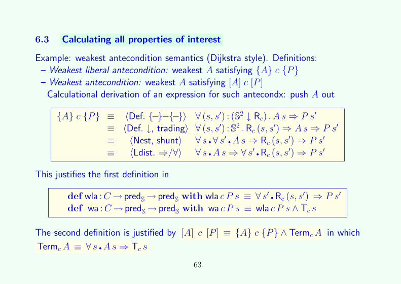
6.3 Calculating all properties of interest

Example: weakest antecondition semantics (Dijkstra style). Definitions:– Weakest liberal antecondition: weakest A satisfying {A} c {P}– Weakest antecondition: weakest A satisfying [A] c [P ]Calculational derivation of an expression for such antecondx: push A out

{A} c {P} ≡ 〈Def. {−}−{−}〉 ∀ (s, s′) : (S2 ↓ Rc) . A s⇒ P s′

≡ 〈Def. ↓, trading〉 ∀ (s, s′) : S2 .Rc (s, s′) ⇒ As⇒ P s′

≡ 〈Nest, shunt〉 ∀ s • ∀ s′ •As⇒ Rc (s, s′) ⇒ P s′

≡ 〈Ldist. ⇒/∀〉 ∀ s •As⇒ ∀ s′ • Rc (s, s′) ⇒ P s′

This justifies the first definition in

def wla :C→ predS→ predS with wla c P s ≡ ∀ s′ • Rc (s, s′) ⇒ P s′

def wa :C→ predS→ predS with wa c P s ≡ wla c P s ∧ Tc s

The second definition is justified by [A] c [P ] ≡ {A} c {P} ∧ TermcA in which

TermcA ≡ ∀ s •As⇒ Tc s

63

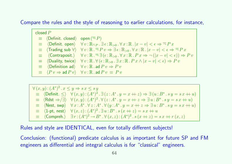
Compare the rules and the style of reasoning to earlier calculations, for instance,

closedP≡ 〈Definit. closed〉 open (¬P )≡ 〈Definit. open〉 ∀ v : R¬P .∃ ε : R>0 .∀x : R . |x− v| < ε⇒ ¬P x≡ 〈Trading sub ∀〉 ∀ v : R .¬P v ⇒ ∃ ε : R>0 .∀x : R . |x− v| < ε⇒ ¬P x≡ 〈Contraposit.〉 ∀ v : R .¬∃ (ε : R>0 .∀x : R . P x⇒ ¬ (|x− v| < ε)) ⇒ P v≡ 〈Duality, twice〉 ∀ v : R .∀ (ε : R>0 .∃x : R . P x ∧ |x− v| < ε) ⇒ P v≡ 〈Definition ad〉 ∀ v : R . adP v ⇒ P v≡ 〈P v ⇒ adP v〉 ∀ v : R . adP v ≡ P v

∀ (x, y) : (A∗)2 . x ≤ y ⇒ s x ≤ s y≡ 〈Definit. ≤〉 ∀ (x, y) : (A∗)2 .∃ (z :A∗ . y = x++ z) ⇒ ∃ (u :B∗ . s y = s x++u)≡ 〈Rdst ⇒/∃〉 ∀ (x, y) : (A∗)2 .∀ (z :A∗ . y = x++ z ⇒ ∃u :B∗ . s y = s x++u)≡ 〈Nest, swp〉 ∀x :A∗ .∀ z :A∗ .∀ (y :A∗ . y = x++ z ⇒ ∃u :B∗ . s y = s x++u)≡ 〈1-pt, nest〉 ∀ (x, z) : (A∗)2 .∃u :B∗ . s (x++ z) = s x++u≡ 〈Compreh.〉 ∃ r : (A∗)2→B∗ .∀ (x, z) : (A∗)2 . s (x++ z) = s x++ r (x, z)

Rules and style are IDENTICAL, even for totally different subjects!

Conclusion: (functional) predicate calculus is as important for future SP and FMengineers as differential and integral calculus is for “classical” engineers.

64

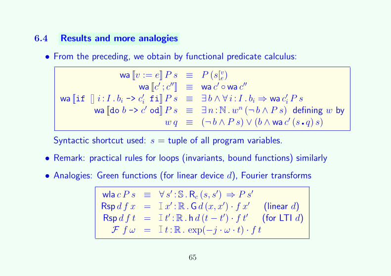
6.4 Results and more analogies

• From the preceding, we obtain by functional predicate calculus:

wa [[v := e]]P s ≡ P (s[ve)wa [[c′ ; c′′]] ≡ wa c′ ◦wa c′′

wa [[if i : I . bi -> c′i fi]]P s ≡ ∃ b ∧ ∀ i : I . bi ⇒ wa c′i P s

wa [[do b -> c′ od]]P s ≡ ∃n : N . wn (¬ b ∧ P s) defining w byw q ≡ (¬ b ∧ P s) ∨ (b ∧ wa c′ (s • q) s)

Syntactic shortcut used: s = tuple of all program variables.

• Remark: practical rules for loops (invariants, bound functions) similarly

• Analogies: Green functions (for linear device d), Fourier transforms

wla c P s ≡ ∀ s′ : S .Rc (s, s′) ⇒ P s′

Rsp d f x = x′ : R .G d (x, x′) · f x′ (linear d)Rsp d f t = t′ : R . h d (t− t′) · f t′ (for LTI d)F f ω = t : R . exp(−j · ω · t) · f t

65

Next topic

09:00–09:20 0. Motivation: synergy FM-SP; value of defect-free formalismsPart I — Unifying the mathematics of SP and FM

09:20–09:40 1. Review of the basics and outline of the formalism used09:40–10:10 2. Inspiration from SP to FM: functions and functionals10:10–10:30 3. Calculation with predicates and quantifiers for engineers10:30–11:00 (Half-hour break)

Part II — Application examples to modeling in SP and FM11:00–11:40 4. Predicate calculus and generic functionals applied to classical SP11:40–11:45 5. Brief intermezzo about endosemantic functions11:45–12:05 6. Modeling programs by program equations

12:05–12:25 7. Reasoning about temporal behavior by temporal operators

12:25–12:30 8. Final considerations

66

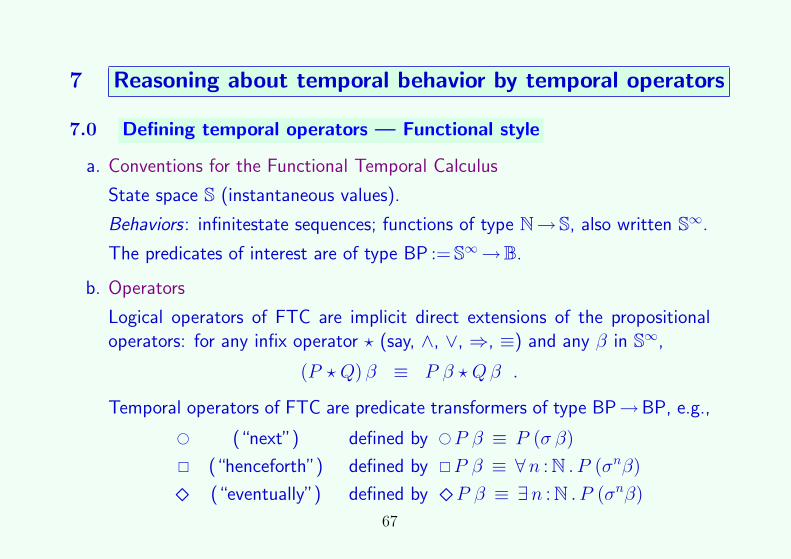
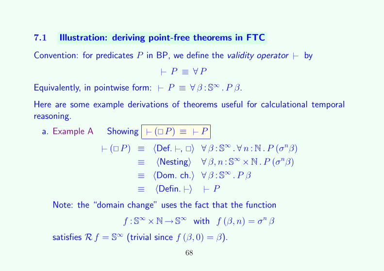
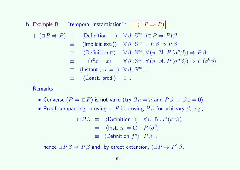
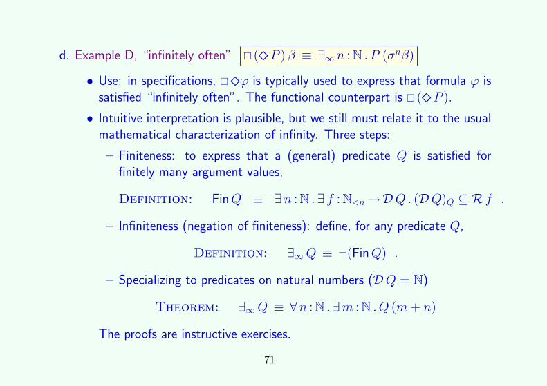
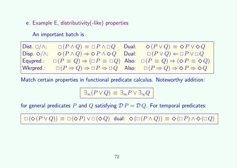
7 Reasoning about temporal behavior by temporal operators

7.0 Defining temporal operators — Functional style

a. Conventions for the Functional Temporal Calculus

State space S (instantaneous values).

Behaviors: infinitestate sequences; functions of type N→S, also written S∞.

The predicates of interest are of type BP := S∞→B.

b. Operators

Logical operators of FTC are implicit direct extensions of the propositionaloperators: for any infix operator ? (say, ∧, ∨, ⇒, ≡) and any β in S∞,

(P ? Q) β ≡ P β ? Qβ .

Temporal operators of FTC are predicate transformers of type BP→BP, e.g.,g (“next”) defined by gP β ≡ P (σ β)

� (“henceforth”) defined by �P β ≡ ∀n : N . P (σnβ)

� (“eventually”) defined by �P β ≡ ∃n : N . P (σnβ)

67

7.1 Illustration: deriving point-free theorems in FTC

Convention: for predicates P in BP, we define the validity operator by

P ≡ ∀P

Equivalently, in pointwise form: P ≡ ∀ β : S∞ . P β.

Here are some example derivations of theorems useful for calculational temporalreasoning.

a. Example A Showing (�P ) ≡ P

(�P ) ≡ 〈Def. , �〉 ∀ β : S∞ .∀n : N . P (σnβ)

≡ 〈Nesting〉 ∀ β, n : S∞×N . P (σnβ)

≡ 〈Dom. ch.〉 ∀ β : S∞ . P β≡ 〈Defin. 〉 P

Note: the “domain change” uses the fact that the function

f : S∞×N→S∞ with f (β, n) = σn β

satisfies R f = S∞ (trivial since f (β, 0) = β).

68

b. Example B “temporal instantiation”: (�P ⇒ P )

(�P ⇒ P ) ≡ 〈Definition 〉 ∀ β : S∞ . (�P ⇒ P ) β

≡ 〈Implicit ext.)〉 ∀ β : S∞ .�P β ⇒ P β

≡ 〈Definition �〉 ∀β : S∞ .∀ (n : N . P (σnβ)) ⇒ P β

≡ 〈f 0x = x〉 ∀ β : S∞ .∀ (n : N . P (σnβ)) ⇒ P (σ0β)

≡ 〈Instant., n := 0〉 ∀ β : S∞ . 1≡ 〈Const. pred.〉 1 .

Remarks

• Converse (P ⇒ �P ) is not valid (try β n = n and P β ≡ β 0 = 0).

• Proof compacting: proving P is proving P β for arbitrary β, e.g.,

�P β ≡ 〈Definition �〉 ∀n : N . P (σnβ)

⇒ 〈Inst. n := 0〉 P (σ0)

≡ 〈Definition fn〉 P β ,

hence �P β ⇒ P β and, by direct extension, (�P ⇒ P ) β.

69

c. Example C: temporal induction (� (P ⇒ gP ) ≡ � (P ⇒ �P )) (STI)

Interest: proof uses a nice generalization of weak induction over N (WIN),called strengthened weak induction (SWIN). For comparison:

∀ (n : N . Qn⇒ Q (n+ 1)) ⇒ Q 0 ⇒ ∀m : N . Qm (WIN)

∀ (n : N . Qn⇒ Q (n+ 1)) ≡ ∀n : N . Qn⇒ ∀m : N . Q (n+m) (SWIN)

Deriving (STI) from (SWIN) is a straightforward exercise.

70

d. Example D, “infinitely often” � (�P ) β ≡ ∃∞ n : N . P (σnβ)

• Use: in specifications, ��ϕ is typically used to express that formula ϕ issatisfied “infinitely often”. The functional counterpart is � (�P ).

• Intuitive interpretation is plausible, but we still must relate it to the usualmathematical characterization of infinity. Three steps:

– Finiteness: to express that a (general) predicate Q is satisfied forfinitely many argument values,

Definition: FinQ ≡ ∃n : N .∃ f : N<n→DQ . (DQ)Q ⊆ R f .

– Infiniteness (negation of finiteness): define, for any predicate Q,

Definition: ∃∞Q ≡ ¬(FinQ) .

– Specializing to predicates on natural numbers (DQ = N)

Theorem: ∃∞Q ≡ ∀n : N .∃m : N . Q (m+ n)

The proofs are instructive exercises.

71

e. Example E, distributivity(-like) properties

An important batch is

Dist. �/∧: � (P ∧Q) ≡ �P ∧ �Q Dual: � (P ∨Q) ≡ �P ∨ �QDisp. �/∧: � (P ∧Q) ⇒ �P ∧ �Q Dual: � (P ∨Q) ⇐ �P ∨ �Q

Equpred.: � (P ≡ Q) ⇒ (�P ≡ �Q) Also: � (P ≡ Q) ⇒ (�P ≡ �Q)Wkrpred.: � (P ⇒ Q) ⇒ �P ⇒ �Q Also: � (P ⇒ Q) ⇒ �P ⇒ �QMatch certain properties in functional predicate calculus. Noteworthy addition:

∃∞(P ∨Q) ≡ ∃∞P ∨ ∃∞Q

for general predicates P and Q satisfying D P = DQ. For temporal predicates:

� (� (P ∨Q)) ≡ � (�P ) ∨ � (�Q) dual: � (� (P ∧Q)) ≡ � (�P ) ∧ � (�Q)

72

Two important observations

• FTC is entirely formulated within functional predicate calculus, without a sep-arate temporal logic language. The operators are predicate transformers.

• FTC captures the essence of temporal logic, and can thereby serve as anarchetype for studying other temporal logics, an issue addressed next.Derivations & results from FTC “carried over”, replacing P β by β ϕ.

Most crucial: FTC “imports” calculational reasoning in temporal logics.

73

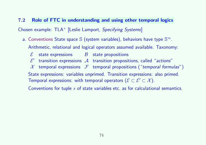
7.2 Role of FTC in understanding and using other temporal logics

Chosen example: TLA+ [Leslie Lamport, Specifying Systems]

a. Conventions State space S (system variables), behaviors have type S∞.

Arithmetic, relational and logical operators assumed available. Taxonomy:

E state expressions B state propositionsE ′ transition expressions A transition propositions, called “actions”X temporal expressions F temporal propositions (“temporal formulas”)

State expressions: variables unprimed. Transition expressions: also primed.Temporal expressions: with temporal operators (E ⊂ E ′ ⊂ X ).

Conventions for tuple s of state variables etc. as for calculational semantics.

74

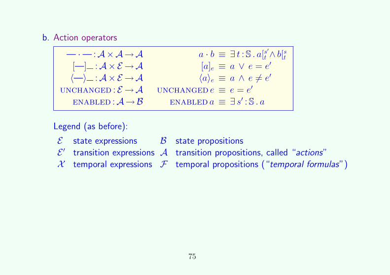
b. Action operators

— ·— :A×A→A a · b ≡ ∃ t : S . a[s′t ∧ b[st[—]— :A×E →A [a]e ≡ a ∨ e = e′

〈—〉— :A×E →A 〈a〉e ≡ a ∧ e 6= e′

unchanged : E →A unchanged e ≡ e = e′

enabled :A→B enabled a ≡ ∃ s′ : S . a

Legend (as before):

E state expressions B state propositionsE ′ transition expressions A transition propositions, called “actions”X temporal expressions F temporal propositions (“temporal formulas”)

75

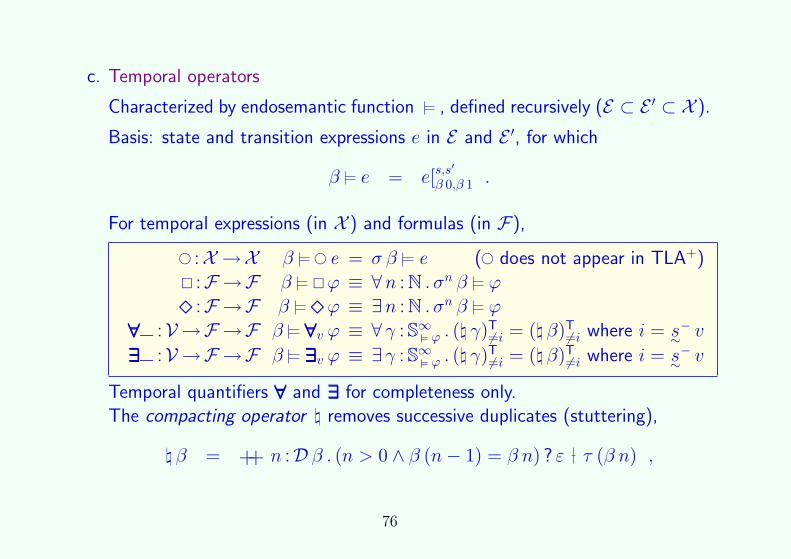
c. Temporal operators

Characterized by endosemantic function , defined recursively (E ⊂ E ′ ⊂ X ).

Basis: state and transition expressions e in E and E ′, for which

β e = e[s,s′

β 0,β 1 .

For temporal expressions (in X ) and formulas (in F),

g:X →X β ge = σ β e ( gdoes not appear in TLA+)

� :F →F β �ϕ ≡ ∀n : N . σn β ϕ

� :F →F β �ϕ ≡ ∃n : N . σn β ϕ

∀∀— :V →F →F β ∀∀v ϕ ≡ ∀ γ : S∞ϕ . (\ γ)T6=i = (\ β)T

6=i where i = ∼s− v

∃∃— :V →F →F β ∃∃v ϕ ≡ ∃ γ : S∞ϕ . (\ γ)T6=i = (\ β)T

6=i where i = ∼s− v

Temporal quantifiers ∀∀ and ∃∃ for completeness only.The compacting operator \ removes successive duplicates (stuttering),

\ β = ++ n :D β . (n > 0 ∧ β (n− 1) = β n) ? ε τ (β n) ,

76

d. Boolean combinations of temporal formulas are defined by distributivity:

β ¬ϕ ≡ ¬ (β ϕ) β ∀ (x :X .ϕ) ≡ ∀x :X . β ϕ

β (ϕ ? ψ) ≡ β ϕ ? β ψ β ∃ (x :X .ϕ) ≡ ∃x :X . β ϕ

Here ? is any infix logical operator in {⇒,≡,≡/ ,⊕,∧,∨}.

Remarks

• To the left of ≡, operators ?, ¬, ∀, ∃ are TLA+; to the right, just logic.

• Because temporal formulas appear only syntactically, we adopt the syntaxof the target language, e.g., optional parentheses: ��ϕ stands for � (�ϕ).

General observation “Proof of the pudding” is not mere survival, but taste.Here this means: elegant calculational reasoning.Experience: approach has replaced semi-formal traditional proofs by formal calcu-lational derivations that are shorter, clearer (structure), and don’t skip steps.

77

Next topic

09:00–09:20 0. Motivation: synergy FM-SP; value of defect-free formalismsPart I — Unifying the mathematics of SP and FM

09:20–09:40 1. Review of the basics and outline of the formalism used09:40–10:10 2. Inspiration from SP to FM: functions and functionals10:10–10:30 3. Calculation with predicates and quantifiers for engineers10:30–11:00 (Half-hour break)

Part II — Application examples to modeling in SP and FM11:00–11:40 4. Predicate calculus and generic functionals applied to classical SP11:40–11:45 5. Brief intermezzo about endosemantic functions11:45–12:05 6. Modeling programs by program equations12:05–12:25 7. Reasoning about temporal behavior by temporal operators

12:25–12:30 8. Final considerations

78

8 Final considerations

• What we have shown

– Notational and methodological unification of CS and classical engineering

– Unification of system modeling and reasoning styles in SP and FM

– Unification also extends to a large part of mathematics

• Ramifications

Generic functionals and (functional) predicate calculus are as important forfuture SP and FM engineers as differential and integral calculus are for“classical” engineers.

79