Formation Evaluation: Carbonate versus SandstoneR. E. (Gene) Ballay and R. (Roy) E. Cox, Consultants
Abstract
The professional geoscientist of today will typically work both sandstone andcarbonate provinces, possibly even simultaneously. Many of the wireline toolsupon which their efforts and results are based, will be the same in bothenvironments, but the utility and underlying physical meaning of the response,may differ between sandstone and carbonate.
By summarizing the key issues, and how the routine open-hole tools respondand are used, one is able to focus their efforts is a more efficient manner. Thereare, of course, exceptions to virtually every rule, which is why experience in aspecific Field is of such value.
Long experience, with many wells successfully drilled, does not of itself eliminatesurprises: Ballay (2001, 2002). In this example, with 120 successful wells (45 ofwhich were cored) drilled, a completely unexpected poor formation wasencountered in an area previously drilled. And so one returns to the value ofunderstanding the basics, and being just as alert with well # 121, as when thefirst well was drilled.
This article summarizes key response attributes and sandstone vs carbonatedifferences for routine open-hole tools. In a later article we plan to examinespecialty tools.
Genesis, Diagenesis and Consequences
The carbonate (ie containing CO3) environment is typically one that has formed‘in place’ via the growth of organisms and / or precipitation. One may alsoencounter evaporates (halite, anhydrite, gypsum) in association with the moreroutine limestone (CaCO3) and dolostone (CaMg(CO3)2 ).
Sandstones (SiO2), on the other hand, are typically clastic in origin and consist offragments of material that were originally deposited elsewhere, broken up andtransported via water or wind, and re-deposited. While carbonates can be clastic,that is much less common than the ‘in place’ origin. In the sandstone world,complications are often associated with ‘clay/shale’, although other issues (suchas feldspar, glauconite) arise in certain provinces.
Clay, silt and shale are the common obstacles present in sandstone formationevaluation. The exact meaning of these terms is sometimes dependent uponlocation, and context, but a general definition is one of grain size, with shalebeing a consolidation of both silt (4 74 um) and clay (< 4 um) sized particles.
Clay usually consists of one (or more) of the following minerals: chlorite, illite,kaolinite and smectite. In contrast to both sand and carbonate, these materialsare electrically conductive, and therein lies one of the fundamental distinctions incarbonate vs sandstone formation evaluation: resistivity will be lowered relativeto the ‘clean sand’ value and thereby give rise to a pessimistic Sw(Archie). Thepresence of clay will also affect the porosity determination, and the compositecorrection for effects on both porosity and saturation is referred to as The ShalySand Problem.
Clay distribution mode, in addition to the volumetric amount, is also an issue -structural, dispersed and laminated – and impacts both the associated electricalcircuit and appropriate adjustment to porosity.
Perhaps surprisingly, the question of dispersed or laminated geometry (poresystems) is also an issue with carbonates (Chris Smart, 2005). In a recentTopical Conference the five most common causes of Low Resistivity Pay inCarbonates were ranked as (most least common):• Dual porosity system (dispersed large and small pores) with the small poresbeing water filled while the larger pores are hydrocarbon charged• Layered formation, in which the large (grainstone, etc) and small (micrite, etc)pore size rock is laminated• Fractures, which may be oil-filled and present in a (small pore) water filledmatrix• Conductive minerals (rare)• Incorrect Rt (excessive invasion, etc) measurement (rare)
Sandstones are then clastic in origin with diagenesis typically limited tocompaction and cementation. Carbonates, which are more soluble in water, haveusually grown in place, and then evolved via cementation, compaction,dolomitization and dissolution (Jerry Lucia, 2004). The importance of dissolutionis immediately apparent in the carbonate outcrops, road cuts and caves of theMidwest USA (Figure 1).
In many regards, the key distinction between sand and carbonate, is thenone of clay effects versus pore size distribution.
SP and Gamma Ray
Spontaneous potential (SP) is the naturally arising voltage difference betweenthe borehole (at a specific depth) and surface, measured in milli-volts (though it isrelative magnitude, and not absolute value, that is important). There will typicallybe Baseline Drift (which should be removed prior to using the data in aquantitative fashion) and a depth-specific Deflection (voltage potential) that is afunction of the difference in Rmf (drilling mud filtrate) Rw (formation brine),and clay content.
In the case of distinctly different Rmf and Rw, and across relatively thick beds,one is often able to use the (baseline straightened) sandstone SP to estimateboth V(Clay) throughout, and formation Rw (in the ‘clean’ intervals).
There is, to our knowledge, no direct, general relation between the magnitude ofSP deflection and the actual value of porosity and / or permeability. It’s rather aV(Clay) indicator, to be fed into the downstream calculations just as otherindicators are.
Carbonates, with their wide range of pore sizes, result in a less well defined SPresponse, and the SP measurement is not even displayed in many CarbonateCountry log suites.
Carbonate versus SandstoneFigure 1
• Carbonate - Diagenesis includes ……...dissolution
• Surface example of how carbonate reservoir rock can be modified.
Natural gamma ray activity arises from three sources: 40K and daughter productsof 232Th and 238U.
In the clastic world, GR activity is often (but not always) a result of clay, andtherefore indicative of a decrease in rock quality. It is for this reason that V(Clay)calculations nearly always include the GR as one estimator (linear as below, orsome other functional form).
Specific clay types have specific relative radioactive components (40K, 232Th,238U), specific GR activities, and can be identified by means of spectral gammaray logs.
When faced with variable clay types, or the possibility of additional radioactivecomponents, it’s a very good idea to supplement the GR V(Shale) estimates withalternatives from the SP and / or Density - Neutron. For example, we have seenshallow horizon clastic intervals (above the expected pay), logged with only GR /SP / Sonic for which there was very little indication of reservoir quality rock by theGR, yet the SP clearly revealed potential (which was validated with production).And in the cleanest of these intervals, Rw(SP) was in agreement withindependently derived values, suggesting that the measurements were valid.
Confusion can arise by failing to clearly distinguish between shale and clay.Bhuyan (1994) found a common error to be the assumption that shales are 100percent clay whereas in fact shales are commonly composed of 50 to 70 percentclay, 25 to 45 percent silt- and clay-sized quartz, and 5 percent other minerals.
In our experience, there is also a tendency to sometimes regard the rock asbeing composed of sand – silt – clay, in the absence of any silt compositionalinformation, and in the face of likely (even verifiable) vertical clay compositionalvariations. We have also found that when the logs are compared to core, arelatively few sedimentary laminations within ‘clean’ sand bodies, can give rise tolog responses that are then interpreted as reflecting a silt interval. One issometimes (but not always) able to work with the more simple sand – shalemodel and develop therefrom 3-D geological models that are just as reasonableas the three component results.
A final word about clastics: KCl mud may be used for borehole stability and willshift the GR upwards: the effect must be accounted for if the GR is to be used forV(Clay).
Uranium-bearing minerals are rare but soluble, transported easily and can beprecipitated far from their source. In carbonates it’s not uncommon to find the GRbeing driven by uranium, in a fashion that is not necessarily indicative of rockquality. The presence of uranium, and the associated higher GR, can signal
stylolites, fractures, super-perm and / or general increases and decreases, inquality (Figure 2). Spectral GR data is particularly useful in the interpretation ofcarbonate GR responses.
In today’s world of highly deviated wells, for which the tools may be pipe-conveyed, one must also be alert for tool-induced GR response (Ballay 1998).The GR module is typically at the top of the string, and when data is acquiredgoing ‘into the hole’, particularly at pipe connection time, the GR response will beaffected by formation activation associated with the other tools (which precedethe GR, in the downwards direction).
Ehrenberg et al (2001) have documented an application of the spectral gammaray in a Barents Sea carbonate.
In many regards, the key distinction between sand and carbonate, is thenthe utility and meaning (or lack thereof) of SP / GR response.
Porosity
Sandstone porosity is normally thought of as consisting of Total and Effective,with the two being related by (or something similar)
• Trend parallel to LS line, but offset• Pef is qualitative, not quantitative• Higher GR corresponds to better qualitylimestone and increase in dolomitization• Black points are invalid data (ie ignore)
•Uranium has been removed!•Limestone generally clean, throughout
•LS GR activity was essentially alluranium
•Dolomite is higher non-uranium GR activity•Did dolomitization occur in rock whichwas depositionally different?
The porosity difference is clay-bound water, which will appear as ‘porosity’ to thelogging tools. Since this ‘water’ is in fact immobile, not to be displaced byhydrocarbon, the associated pore volume is referred to as ineffective.
Common porosity estimators are the density, neutron and sonic, usedindividually, in tandem or all three together.
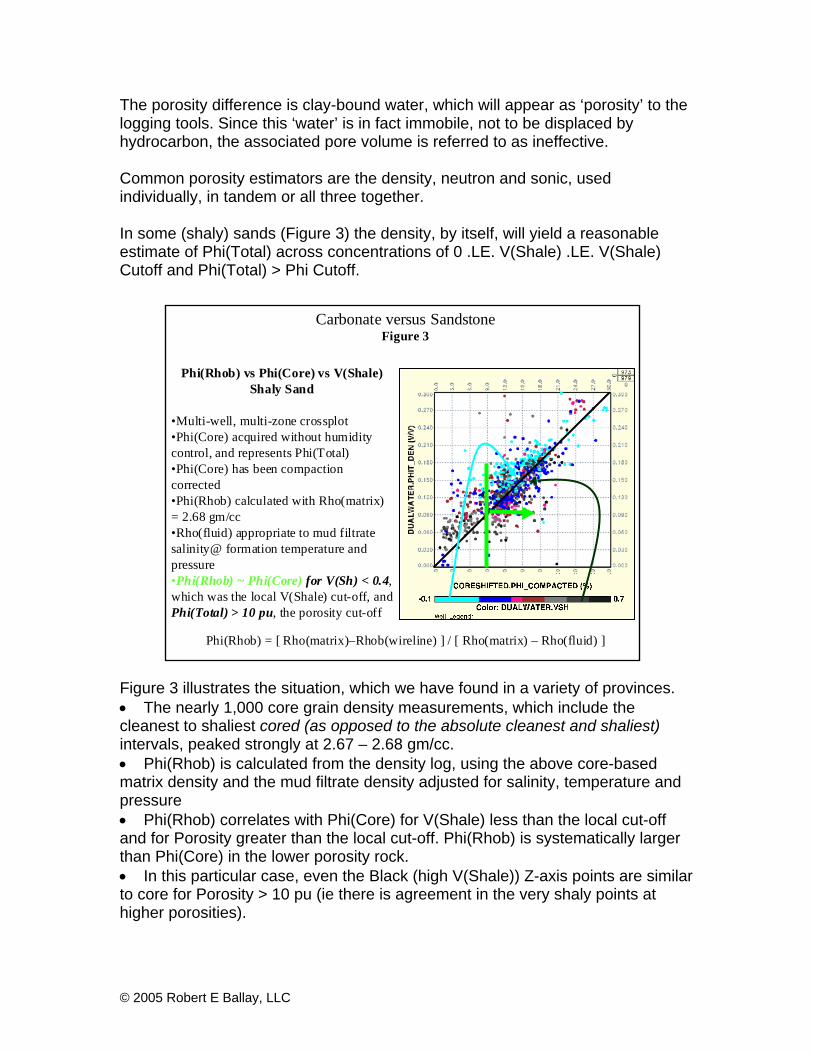
In some (shaly) sands (Figure 3) the density, by itself, will yield a reasonableestimate of Phi(Total) across concentrations of 0 .LE. V(Shale) .LE. V(Shale)Cutoff and Phi(Total) > Phi Cutoff.
Figure 3 illustrates the situation, which we have found in a variety of provinces.• The nearly 1,000 core grain density measurements, which include thecleanest to shaliest cored (as opposed to the absolute cleanest and shaliest)intervals, peaked strongly at 2.67 – 2.68 gm/cc.• Phi(Rhob) is calculated from the density log, using the above core-basedmatrix density and the mud filtrate density adjusted for salinity, temperature andpressure• Phi(Rhob) correlates with Phi(Core) for V(Shale) less than the local cut-offand for Porosity greater than the local cut-off. Phi(Rhob) is systematically largerthan Phi(Core) in the lower porosity rock.• In this particular case, even the Black (high V(Shale)) Z-axis points are similarto core for Porosity > 10 pu (ie there is agreement in the very shaly points athigher porosities).
Phi(Rhob) vs Phi(Core) vs V(Shale)Shaly Sand
•Multi-well, multi-zone crossplot•Phi(Core) acquired without humiditycontrol, and represents Phi(Total)•Phi(Core) has been compactioncorrected•Phi(Rhob) calculated with Rho(matrix)= 2.68 gm/cc•Rho(fluid) appropriate to mud filtratesalinity@ formation temperature andpressure•Phi(Rhob) ~ Phi(Core) for V(Sh) < 0.4,which was the local V(Shale) cut-off, andPhi(Total) > 10 pu, the porosity cut-off
This fortuitous event happens because• Rho(matrix) of sand and shale are locally similar in magnitude (in spite of thesignificant variations reported in various reference summaries), and/or• The ‘limited range of calibration / applicability’ of the method (ie within paycut-offs) has restricted the evaluation to the domain in which the assumption isvalid (which would appear to be the situation in Figure 3.
An alternative porosity estimator is the neutron log, which is subject to manymore environmental corrections (than is the density), in addition to experiencinga relatively larger shale effect and potentially large light hydrocarbonsuppression. If a valid neutron log is available, the density-neutron combinationoffers a common solution to the shaly sand porosity problem.
The third routine porosity estimator is the sonic log, which requires noenvironmental correction, but like the neutron, will often be more sensitive toshale. One should also be aware of the ‘adjustments’ to the acoustical porositythat may be necessary in ‘soft rock’ country: sometimes in country that is notthought of as soft rock.
Per the Schlumberger Principles Manual, and observed in our own experience, ifthe bounding shales have ∆ t > 100 us/ft, both of the common porosity transforms(Wyllie and Field Observation) may require a correction factor. ∆ t (Shale) ~ 90=> 100 us/ft may not be thought of as soft rock country, yet we have encounteredcore – log comparisons which demonstrated the need for the compactionadjustment.
Carbonate porosity (Jerry Lucia, 2004) determination, as contrasted tosandstone, is a completely different issue. Now one is faced with Interparticle(intergrain and intercrystal), and Vuggy porosity. Vuggy porosity is everythingthat is not interparticle, and includes vugs, molds and fractures. Vugs are dividedinto separate and touching.
One sometimes encounters the Phi(Total) / Phi(Effective) terminology in thecarbonate literature, but the meaning of these terms is now related to irreduciblecapillary pressure water saturations, and not clay-bound water. For example,Melas et al (1992) define Phi(Effective) = Phi(Total)*(1-Swi), in their study of theSmackover.
Porosity estimates in the carbonate world must often allow for a mix of minerals -limestone and dolostone with distinctly different grain densities - plus possiblyanhydrite and halite. Determination of component percentages now requiresmultiple measurements and equations: two components require twomeasurements, etc.
The neutron-density combination is the common tool of choice (Figures 4 and 5)
In Figure 4 the z-axis is annotated with water saturation, as a check for lighthydrocarbon effects on the porosity estimate (note that Sw drops to less than10%).
Φ(Rhob/NPhi) vs Φ(Core) vs SwCarbonate
•Multi-well, multi-zone crossplot•Phi(Core) acquired without humiditycontrol, and represents Phi(Total), butthere is no ‘shale’ issue in this reservoir•Phi(Core) has not been compactioncorrected, but that factor is relativelysmall in this ‘hard rock country’• Φ(Rhob/NPhi) ~ Φ(Core) across a widerange of Sw (z axis), thereby verifyingthe absence of light hydrocarbon effects
•Depth orientedsingle well display•Wirelinemineralogy varies inaccordance withcore attributes•Towards the baseof the well, coregrain density &porosity are affectedby incompletecleaning & drying)
Light hydrocarbon effects on the porosity estimate are an issue in bothsandstones and carbonates, and in both environments we have found• The density will be less affected than the neutron (common knowledge)• In single mineral environments, Phi(Rhob) estimated with mud filtrateattributes (ie complete flushing), will match core better than the commonlyreported iterative approach (calculate Phi, calculate Sxo, calculate weightedaverage invaded zone fluid density, re-calculate Phi, etc until the ∆ Porosity periteration reaches some pre-set value.)• Although the iterative correction for light hydrocarbons makes logical sense, itmay be that the different vertical resolutions and depths of investigation of theindependent measurements that go into the iteration have compromised it. In anycase, comparisons to core in both sandstone and carbonate reservoirs haveshown that the simpler (assume complete flushing) Phi(Rhob) estimate is abetter match. If one wishes to implement iteration, they should consider haltingthe iteration at some pre-determined point, but prior to convergence, in whichcase we have been able to achieve matches to core.• If multiple minerals are present, multiple input measurements will be requiredand this ‘simple’ Phi(Rhob) method will not suffice.
In addition to the multiple mineral problem, we have also found LWD Rhobmeasurements, just behind the bit, for which the simple (Rhob) porosity estimatewill not be realistic. Now light hydrocarbon effects that would not be nearly soevident with wireline data, which is acquired relatively longer after bit penetrationand thereby allows more filtrate invasion to take place, can be apparent. In thiscase our preference is a probabilistic approach if the software is available.
The need to distinguish between interparticle and vuggy porosity, will require theintroduction of an additional independent tool (an additional dimension requiresan additional input), and the sonic is often the (routine) tool of choice.
An early documentation of this capability is due to Wyllie (1958), in which heplotted measured dolomite core porosity (intercrystalline, vuggy, fracture) versuscompressional transit time, and observed the intercrystalline response to fallalong the expected time average equation trend line, whereas the other ‘ porositytypes’ were not ‘fully seen’.
Conceptually, the radioactive tools respond to all porosity, while the acousticalwaves are more pore size dependent. John Rasmus (1983) used a comparisonof Phi(Rhob/Nphi) – Phi(Sonic) – Core to illustrate the effect with actual data.
Anselmetti et al (1999) and Eberli et al (2003) have followed-up on this questionto find that “moldic porosity exhibits a range or responses that varies fromintercrystalline - interparticle to intraframe”.
• Not all deviations from the Wyllie time-average equation are caused byseparate-vug porosity• Not all separate-vug pore space causes deviations from the Wyllie curve• Careful testing and calibration with core data will be required for eachcarbonate reservoir
Physically, there is a scattering that takes place in the acoustic waves, similar tothat modeled by John Rasmus et al (1985) in the dielectric log: the contrast ofdielectric and resistivity responses in rock that ranges from intercrystalline /interparticle to vuggy can be used to characterize the porosity type.
The dielectric will ‘see’ the vuggy oomoldic porosity more effectively thanresistivity, since dielectric response does not depend on pore connectivity, butthe contribution is not (initially) 100 % (John Rasmus, 2004) – “The ribs arecaused by the "scattering" effect of the inclusions on the electromagnetic wave.There is a similar effect on sonic waves. Alain Brie has shown that the sonic"sees" approximately 20-30% of the inclusions in addition to the intergranularporosity”.
Whether working in the carbonate or sandstone world, it’s important to be alertfor data integrity issues. In a 41 well carbonate study, drawing upon more than30,000 core measurements, we (Ballay, 1994) found• 22 % of the Sonic Logs Required Adjustment (~ 1 pu)
• This reservoir was generally non-vuggy, interparticle / intercrystallineporosity and pore type did not play a role in the QC
• 51 % of the Density Logs Required Adjustment (~ 1 pu)• Constant Shift Usually Sufficient
• 88 % of the Neutron Logs Required Attention• Usually small (~ 1 pu) shifts at low porosity, but large (4 - 6 pu in 30 purock) in high quality rock. Part of this was light hydrocarbon effect, but themagnitude was far beyond what either of the two sets of Service Companydocuments would have predicted, and was never explainable in aquantitative manner.
Halite, if present, requires that one be aware of how the density measurement isactually accomplished. Most, but not all, elements have an Atomic Number /Atomic Mass ratio of very close to 2.0. Silicon and Oxygen, for example, are 2.01and 2.00 respectively. Salt, on the other hand, does not satisfy this ratio and sothe wireline-measured bulk density departs from the actual.
In certain areas of the world, anhydrite beds are widespread and referenced forlog QC purposes. In doing so, one should realize that ‘chicken wire’ appearingimpurities are not uncommon, are not present in the same concentrations fromone well to the next, and can give rise to genuine variations in log response.
There is, finally, the question of the benchmark for porosity estimation: the core.Although the grain density is typically determined as a part of the lab procedure,it may not be included in the reported tabulations (particularly in the olderreports). When included, its usefulness may not be recognized by the interpreter.
The laboratory measured grain density should be used to quality control both thecore data and the log interpretations. If the reservoir is known to consist oflimestone and dolostone, Rhog(Core) < 2.71 gm/cc should raise a red flag: thecore may not have been completely cleaned or dried (Figure 5). Cleaning is anobvious issue in tar but can present a challenge in lighter oils as well. We havealso found residual salt, in the core plugs, which shifts the measured graindensity downwards.
In many regards, the key distinction between sand and carbonate, is thenone of correcting for clay ‘porosity’ versus allowing for multiple mineralsand pore sizes.
Water Saturation and the Archie Equation
In light of the differences in sandstone and carbonate, per the above discussion,it is perhaps surprising that water saturation can (often) be successfullyestimated with the same equation and (similar) parameters (Figure 6).
From this (Figure 6), and similar, measurements Archie (1947) observed that thecorrelation between Formation Factor (ratio of water saturated rock resistivity tosaturating fluid resistivity) and permeability was weaker than that of FF andporosity, which suggested to him that air permeability and ionic (resistivity) flowwere ‘different’.
Archie’s equation, and the impact of variations in the associated parameters, canbe visualized with a Pickett Plot (Roberto Aguilera 2002, 2004 and Ross Crainon-line at http://www.spec2000.net/ and John Doveton on-line athttp://www.kgs.ku.edu/Gemini/)
Archie’s 1947 Data - Sandstone and Limestone
G E Archie : Electrica l Resistivity as an Aid in Core Analysis Interpretation, AAPG Bulletin 31 (1947): 350-366Schlumberger Technical Review Volume 36 Number 3
Considering, for the moment, ‘clean’ sand and ‘intercrystalline / interparticlecarbonates’, the cementation exponent reflects the tortuosity of the ionicelectrical flow through brine saturated rock. An ‘m’ of 2.0 is commonly used:smaller values correspond to a less tortuous path, with fractures being asomewhat extreme example. Should the path be ‘extra’ tortuous, such as whenthe pore throats are well-cemented, or a portion of the porosity is poorlyconnected vugs, ‘m’ will increase.
Be aware, however, that small pores, by themselves, don’t necessarily meanhigh ‘m’: it is the ‘effectiveness’ of the conduction path.
The cementation exponent of both clean sand and IC/IP carbonates may varywithin a relatively short (vertical) distance, and can assume a multitude of valueswithin a given reservoir. This potential must be recognized, in order to avoidconsolidating data that is in fact ‘different’. These differences may, or may not,correspond to the original depositional environment.
In the words of Jerry Lucia (2004): the foundation of the Lucia petrophysicalclassification is the concept that pore-size distribution controls permeability andsaturation and that pore-size distribution is related to rock fabric. The focus ofthis classification is on petrophysical properties and not genesis. To determinethe relationships between rock fabric and petrophysical parameters, one mustdefine and classify pore space as it exists today in terms of petrophysicalproperties.
Pickett Plot (m=2.5/n=2.0)
0.01
0.10
1.00
0.01 0.10 1.00 10.00 100.00Resistivity
Por
osity Sw=1.00
Sw=0.5Sw=0.3Sw=0.15BVW=0.015BVW=0.03BVW=0.10
Pickett Plot with BVW Grids
•m=2.0 / n=2.0 vs m=2.5 / n=2.0
•‘m’ relates to pore system tortuosity,and as ‘m’ increases, the resistivityof a specific porosity (10 pu in thegraphic) at Sw = 100 % alsoincreases
•Rw @ FT remains the same
•Grids of constant BVW shift
•BVW lines below Sw = 100 % are amathematical extrapolation (for visualreference) and not physically realistic
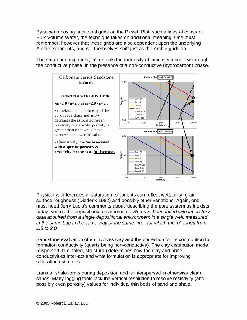
By superimposing additional grids on the Pickett Plot, such a lines of constantBulk Volume Water, the technique takes on additional meaning. One mustremember, however that these grids are also dependent upon the underlyingArchie exponents, and will themselves shift just as the Archie grids do.
The saturation exponent, ‘n’, reflects the tortuosity of ionic electrical flow throughthe conductive phase, in the presence of a non-conductive (hydrocarbon) phase.
Physically, differences in saturation exponents can reflect wettability, grainsurface roughness (Diederix 1982) and possibly other variations. Again, onemust heed Jerry Lucia’s comments about ‘describing the pore system as it existstoday, versus the depositional environment’. We have been faced with laboratorydata acquired from a single depositional environment in a single well, measuredin the same Lab in the same way at the same time, for which the ‘n’ varied from1.5 to 3.0.
Sandstone evaluation often involves clay and the correction for its contribution toformation conductivity (quartz being non-conductive). The clay distribution mode(dispersed, laminated, structural) determines how the clay and brineconductivities inter-act and what formulation is appropriate for improvingsaturation estimates.
Laminar shale forms during deposition and is interspersed in otherwise cleansands. Many logging tools lack the vertical resolution to resolve resistivity (andpossibly even porosity) values for individual thin beds of sand and shale.
Pickett Plot (m=2.0/n=2.5)
0.01
0.10
1.00
0.01 0.10 1.00 10.00 100.00Resistivity
Poro
sity Sw=1.00
Sw=0.5Sw=0.3Sw=0.15BVW=0.015BVW=0.03BVW=0.10
Pickett Plot with BVW Grids
•m=2.0 / n=2.0 vs m=2.0 / n=2.5
•‘n’ relates to the tortuosity of theconductive phase and as Swdecreases the associated rise inresistivity of a specific porosity isgreater than what would haveoccurred at a lower ‘n’ value.
•Alternatively, the Sw associatedwith a specific porosity &resistivity increases as ‘n’ increases
Intervals with dispersed clays are formed during the deposition of individual clayparticles or masses of clay. Dispersed clays can also result from postdepositional processes, such as burrowing and diagenesis. The size differencebetween dispersed clay grains and framework grains allows the dispersed claygrains to line or fill the pore throats between framework grains. When clay coatsthe sand grains, the irreducible water saturation of the formation increases,dramatically lowering resistivity values. If such zones are completed, however,water-free hydrocarbons may be produced.
Structural clays occur when framework grains and fragments of shale or clay,with a grain size equal to or larger than the framework grains are depositedsimultaneously. Alternatively, in the case of selective replacement, diagenesiscan transform framework grains, like feldspar, into clay. Unlike dispersed clays,structural clays act as framework grains without the dramatic altering of reservoirproperties. None (very little) of the pore space is occupied by clay.
Dispersed clay is the most common distribution that we have been faced with(though laminated is certainly a problem in some provinces), and can beaddressed with the Dual Water Model, Waxman-Smits, or several other moreempirical algorithms (Worthington has authored several nice reviews). Thepresence of the clay offers an ‘alternative’ electrical path and therebycompromises the Archie estimates (Archie water saturations will be high). Interms of the Pickett Plot, data points shift to the South West, and so it’s goodpractice to annotate one’s Pickett Plot with SP / GR / Rhob-NPhi / etc in the ‘z’direction.
Roberto Aguilera (1990) developed variations of the shaly sand Pickett Plotwhich offer the option of ‘countering’ the South West shift of data. He found thatall published methods for evaluation of laminar, dispersed and structural clayscould be written as Rt/A_shale = a Rw Phi(effective)^(-m) Sw^(-n) where A_shaleis model dependent (Indonesian, Dual Water, Waxman Smits, etc.....).
If one then displays Rt/A_shale vs Phi(effective), as compared to measuredresistivity vs porosity - Figure 7 & 8, there is a graphical compensation for clayconductivity effects on the resulting (pseudo) Pickett Plot.
As compared to sandstones, the carbonate pore system is less often affected byclay conductivity and one is most commonly faced with variations in the pore sizedistribution / connectivity (Figure 9 and John Rasmus, 1986)
Now the Pickett Plot ‘z’ axis should be annotated with attributes [φ(sonic) vsφ(Rhob/NPhi), etc] that will highlight this characteristic, if present. At the extreme,one may need to supplement the porosity – resistivity evaluation with alternativetechniques (image logs, dielectric log, pulsed neutron log, nuclear magneticresonance, etc).
Schlumberger has published, in their Technical Review / Oilfield Review, threearticles which provide a more in-depth review of Archie’s equation.
• Archie’s Law: Electrical Conduction in Clean, Water-bearing Rock. TheTechnical Review: Volume 36 Number 3• Archie II: Electrical Conduction in Hydrocarbon-Bearing Rock. The TechnicalReview: Volume 36 Number 4• Archie III: Electrical Conduction in Shaly Sands. Oilfield Review: Volume 1Number 3
In many regards, the key distinction between sand and carbonate, is thenone of accounting for clay conductivity ‘short circuits’ versus variations inpore system tortuosity associated with changes from intercrystalline /interparticle to vuggy porosity.
• Unconnected vuggy porespace vs total porosity
• m ~ 2 for interparticleporosity
• m ~ 3 for porosity that is60% vuggy
F J Lucia: Petrophysical Parameters Estimated from Visual Descriptions of Carbonate Rocks: A Field Classification ofCarbonate Pore Space, Journal of Petroleum Technology 35 (1983): 629 - 637Schlumberger Technical Review, Volume 36 Number 3
Development of a single-well evaluation, even one that involves core, is only thebeginning. Formation attributes derived from individual well analyses must fit intothe prevailing geologic framework, well to well: the static model.
Time-lapse monitor logs and production data must be understandable within thecontext of the static model: the fourth dimension.
It’s entirely possibly that the static model will evolve as more wells, and perhapsroutine and special core data, become available, which brings one to an iterativeloop (Ballay, 2000).
Some Companies (Petronas, for example) have a policy of re-examining allFields on a scheduled, rotating basis, taking a fresh look at all (historical andnewly acquired, simultaneously) data. In these time-lapse efforts it’s important torealize that even the routine tools may yield information that was not extractedthe first (or second) time around. Without meaning to discount the value of new,high-tech tools in any way, there are many examples of significant advancesresulting from multi-well studies based upon ‘routine’ tools
In both the sandstone and carbonate worlds, there is tremendous value inmulti-well evaluations and time-lapse comparisons, on a re-occurringschedule.
Summary
Evaluation of sandstones and carbonates typically bring different issues to theforefront. As the geoscientist of today moves from one province to another, it’sworthwhile to summarize those key differences, and thereby focus one’sattention.
This particular contrast has addressed the routine wireline tools. Additional ideasand techniques may be found on-line, at the following links.
We appreciate Roberto Aguilera, Ross Crain, John Doveton, Jerry Lucia, JohnRasmus and Chris Smart’s review of this effort. Roberto’s comments about shalysand Pickett Plots, and Ross’ experience with shaly sand porosity estimatesbrought forward perspectives and ideas that were not in the original version, buthave now been incorporated.
Much of this material was extracted from the Carbonate Petrophysics course thatwas developed, and is taught by, Gene Ballay. He gratefully acknowledges the47 contributors to that effort, who are individually listed in the Introduction Moduleof the Course.
References
• Aguilera, Roberto, 1990, Extensions of Pickett plots for the analysis of shalyformations by well logs: The Log Analyst, v. 31, no. 6, p. 304-313• Aguilera, Roberto , Incorporating capillary pressure, pore throat aperture radii,height above free-water table, and Winland r35 values on Pickett plots. AAPGBulletin, v. 86, no. 4 (April 2002), pp. 605–624• Aguilera, Roberto, Integration of geology, petrophysics, and reservoirengineering for characterization of carbonate reservoirs through Pickett plots.AAPG Bulletin, v. 88, no. 4 (April 2004), pp. 433–446• Anselmetti, Flavio S. et al, The Velocity-Deviation Log: A Tool to Predict PoreType and Permeability Trends in Carbonate Drill Holes from Sonic and Porosityor Density Logs. AAPG Bulletin, V. 83, No. 3 (March 1999), 450–466.• Archie, G E, Electrical Resistivity as an Aid in Core Analysis Interpretation,AAPG Bulletin 31 (1947): 350-366. Schlumberger Technical Review, Volume 36Number 3• Ballay, Gene et al, Porosity Log Quality Control and Interpretation in a HighPorosity Carbonate Reservoir. SPWLA Paper 1994 E• Ballay, Gene et al Up versus Down: Pipe-Conveyed Wireline Data Quality,Dhahran SPE Conference, 1998.• Ballay, Gene, Multi-dimensional Petrophysics in the Reservoir DescriptionDivision. Saudi Aramco Journal of Technology, 2000• Ballay, Gene et al, In the Driver’s Seat with LWD Azimuthal Density Images.SPE 72282, 2001• Ballay, Gene et al, In the Driver’s Seat with LWD Azimuthal Density Images.Saudi Aramco Journal of Technology, 2002 (has more detail than the above SPEpaper)• Bhuyan, K. et al, Clay Estimation from GR and Neutron-Density Logs.SPWLA Thirty-Fifth Annual Logging Symposium, June 19-22, 1994• Diederix, K M, Anomalous Relationships Between Resistivity Index and WaterSaturations in the Rotliegend Sandstone (The Netherlands), Transactions of theSPWLA 23rd Annual Logging Symposium, Corpus Christi, Texas, July 6-9, 1982,Paper X
• Eberli, Gregor P et al, Factors controlling elastic properties in carbonatesediments and rocks. The Leading Edge, July 2003• Ehrenberg, S N et al, Use of spectral gamma-ray signature to interpretstratigraphic surfaces in carbonate strata: An example from the Finnmarkcarbonate platform (Carboniferous–Permian), Barents Sea. AAPG Bulletin, v. 85,no. 2 (February 2001), pp. 295–308• Jennings, James et al. Predicting Permeability From Well Logs in CarbonatesWith a Link to Geology for Interwell Permeability Mapping. SPE 71336. Y2001• Lucia, Jerry Personal communication, 2004• Lucia, Jerry, Rock-Fabric/Petrophysical Classification of Carbonate PoreSpace for Reservoir Characterization. AAPG Bulletin, V. 79, No. 9 (September1995), P. 1275–1300• Lucia, Jerry, Petrophysical parameters estimated from visual description ofcarbonate rocks: a field classification of carbonate pore space: Journal ofPetroleum Technology, March 1983, v. 35, p. 626–637.• Melas, FF et al, Petrophysical Characteristics of the Jurassic Smackover,AAPG V 76 No 1 (Jan 1992)• Pickett, G R, A Review of Current Techniques for Determination of WaterSaturation from Logs," paper SPE 1446, presented at the SPE Rocky MountainRegional Meeting, Denver, Colorado, USA, May 23-24, 1966; SPE Journal ofPetroleum Technology (November 1966): 1425-1435.• Rasmus, John, Personal communication, 2004• Rasmus, John, A Summary of the Effects of Various Pore Geometries andtheir Wettabilities on Measured and In-situ Values of Cementation and SaturationExponents. SPWLA Twenty-seventh Annual Logging Symposium, June 1986• Rasmus, John et al, An Improved Petrophysical Evaluation of OomoldicLansing-Kansas City Formations Utilizing Conductivity and Dielectric LogMeasurements, Transactions of the SPWLA 26th Annual Logging Symposium,Dallas, June 17-20, 1985, Paper V• Rasmus, J C, A Variable Cementation Exponent, m, for FracturedCarbonates, The Log Analyst 24, No 6 (Nov-Dec, 1983):13-23• Schlumberger Oilfield Glossary• Smart, Chris. Personal communication per Topical Conference on LowResistivity Pay in Carbonates, Abu Dhabi, 30th Jan. – 2nd Feb. 2005• Worthington, Paul F, Effect of Variable Saturation Exponent on the Evaluation ofHydrocarbon Saturation, SPE Formation Evaluation, December 1992• Worthington, Paul F, Improved Quantification of Fit-for-Purpose SaturationExponents, August 2004 SPE Reservoir Evaluation & Engineering• Worthington, Paul F, Determination of Fit-for-Purpose Saturation Exponents,paper SPE 71723 presented at the 2001 SPE Annual Technical Conference• Wyllie, M R J et al, An Experimental Investigation of Factors Affecting ElasticWave Velocities in Porous Media. Geophysics (1958) 23,459 - 93