UQ\950-14 Tasmania Department Of Resources and Energy Division of Mines and Mineral Resources - Report 1990/14 Formation water resistivities in the upper Eastern View Group, Bass Basin by P. W Baillie Abstract A regional study of salinity patterns in Eocene sands of the Bass Basin has shown that salinity tends to decrease with depth, possibly related to a decreasing sand/shale ratio down through the Eocene section. INTRODUCTION The purpose of this report is to present the results of a pilot study to determine geological information from conventional wireline log data using a Macintosh microcomputer and MacLog® software. The study investigated regional patterns of water salinity in the Eocene upper Eastern View Group of the Bass Basin. The Bass Basin, a Late Mesozoic-Cainozoic intracratonic basin trending northwest-southeast between Victoria and northern Tasmania, has an area of approximately 65 000 km 2 , and is almost entirely covered by the waters of Bass Strait, mostly between 30 and 90 m deep. Basin-fill consists of up to 16 km of non-marine and marine sediments and volcanics ranging in age from Late Iurassic(?) to Recent (Robinson, 1974; Brown, 1976; Williamson et al., 1985, 1987; Smith, 1986). The main stratigraphic units in the basin are the Upper Iurassic(?)-Lower Cretaceous non-marine Otway Group, the Upper Cretaceous-Upper Eocene non-marine, marginal marine and marine Eastern View Group, the Upper Eocene marginal-marine Demons Bluff Formation, and the Oligocene-Recent marine Torquay Group (Robinson, 1974; Brown, 1976; Smith, 1986; Williamson et al., 1985, 1987; Baillie and Bacon, 1989). The Eastern View Group is up to 8 km thick, consisting of interbedded sandstone, siltstone, mudstone, coal and volcanics. An unconformity of possible regional extent ("M. diversus Unconformity") has been used to informally divide the Group's upper and lower units (Brown, 1976; Nicholas et al., /981; Baillie and Bacon, 1989). The lower unit comprises dominantly finer-grained sediments of Late Cretaceous to Early Eocene (Lower M. diversus Zone) age, while the overlying upper Eastern View Group is rich in coal and more sandy than the lower division (Brown, 1976). The upper Eastern View Group is postulated to have been deposited within a tide-dominated delta, consisting of a complex mixture of distributary channels, strandline sand bars, peat swamps and shallow lagoons (Baillie and Bacon, 1989). METHODS AND DATABASE To date, 27 offshore exploration wells have been drilled in the basin (fig. 1). Digital log data of all wells has been supplied courtesy of Wiltshire Geological Services, Adelaide. The data, supplied as ASCII files*, was either digitised from original paper logs or, in the case of recent wells (1985-86), directly downloaded from Schlumberger Edit Tapes. The study was carried out using MacLog® software (Bowler, 1987) which consists of four stand-alone applications for log evaluation. The LogData application is used to make MacLog files which contain R t and the other logs. Lithoplots, PreEval, and Eval are applications which make petrophysical calculations from the MacLog data files. The data is first converted from ASCII files into files that MacLog® can understand and manipulate. Using the LogData application, the data is converted first into Real Number files, and then into MacLog files following temperature corrections to the Neutron Porosity log: Figure 2 is an example (from the Seal-l well) of a Maclog file output as a data listing and Figure 3 is a graphic plot of data from the same well. Using the LithoPlots application, apparent formation water resistivities (Rwa) are then calculated using the Hingle crossplot method (Asquith, 1982; Helander, 1983). By limiting the study to clean sands known to be non hydrocarbon-bearing, Rwa then becomes Rw, the true formation water resistivity. In more extensive studies than the present pilot study, or in studies of complex lithology, crossplotting of multiple log responses, together with petrographic data from cores or cuttings may be used to establish relationships between log responses and lithotypes. The present study, however, is limited to relatively simple siliciclastic lithotypes. Two types of crossplots in conjunction with the GR and SP logs were used to determine lithology and to identify clean sand zones. Figure 4 is a neutron-density crossplot (RHOB / NPHl) of a sand from the Chat-l (fig. 1) well-note that V clay as determined from the G R log is indicated numerically on the Z-axis (J represents the cleanest sands, shale if present by 9). Figure 5, utilising the Pe curve (photoelectric cross-section), is an example of a MID (Matrix Identification) crossplot of apparent matrix grain density and the apparent matrix volumetric cross-section (RHOmaa / Umaa). In the example illustrated, it is readily apparent that the clean * It should be noted that Imperial units are used throughout this report, because all older and much of the newer petroleum exploration data is presented in Imperial measurements. REPORT 1990/14
Transcript
UQ\950-14
Tasmania Department Of Resources and Energy
Division of Mines and Mineral Resources - Report 1990/14
Formation water resistivities in the upper Eastern View Group, Bass Basin
by P. W Baillie
Abstract
A regional study of salinity patterns in Eocene sands of the Bass Basin has shown that salinity tends to decrease with depth, possibly related to a decreasing sand/shale ratio down through the Eocene section.
INTRODUCTION
The purpose of this report is to present the results of a pilot study to determine geological information from conventional wireline log data using a Macintosh microcomputer and MacLog® software. The study investigated regional patterns of water salinity in the Eocene upper Eastern View Group of the Bass Basin.
The Bass Basin, a Late Mesozoic-Cainozoic intracratonic basin trending northwest-southeast between Victoria and northern Tasmania, has an area of approximately 65 000 km2, and is almost entirely covered by the waters of Bass Strait, mostly between 30 and 90 m deep. Basin-fill consists of up to 16 km of non-marine and marine sediments and volcanics ranging in age from Late Iurassic(?) to Recent (Robinson, 1974; Brown, 1976; Williamson et al., 1985, 1987; Smith, 1986).
The main stratigraphic units in the basin are the Upper Iurassic(?)-Lower Cretaceous non-marine Otway Group, the Upper Cretaceous-Upper Eocene non-marine, marginal marine and marine Eastern View Group, the Upper Eocene marginal-marine Demons Bluff Formation, and the Oligocene-Recent marine Torquay Group (Robinson, 1974; Brown, 1976; Smith, 1986; Williamson et al., 1985, 1987; Baillie and Bacon, 1989).
The Eastern View Group is up to 8 km thick, consisting of interbedded sandstone, siltstone, mudstone, coal and volcanics. An unconformity of possible regional extent ("M. diversus Unconformity") has been used to informally divide the Group's upper and lower units (Brown, 1976; Nicholas et al., /981; Baillie and Bacon, 1989). The lower unit comprises dominantly finer-grained sediments of Late Cretaceous to Early Eocene (Lower M. diversus Zone) age, while the overlying upper Eastern View Group is rich in coal and more sandy than the lower division (Brown, 1976). The upper Eastern View Group is postulated to have been deposited within a tide-dominated delta, consisting of a complex mixture of distributary channels, strandline sand bars, peat swamps and shallow lagoons (Baillie and Bacon, 1989).
METHODS AND DATABASE
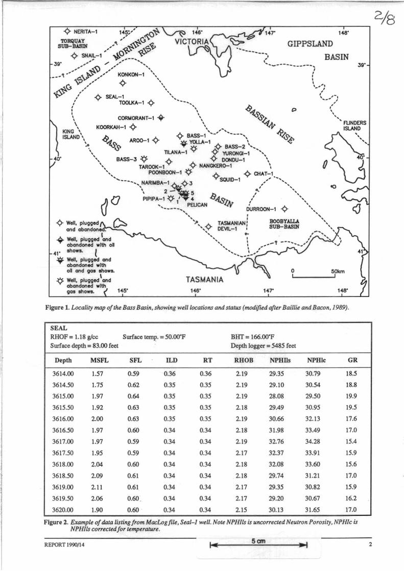
To date, 27 offshore exploration wells have been drilled in the basin (fig. 1). Digital log data of all wells has been supplied courtesy of Wiltshire Geological Services, Adelaide. The data, supplied as ASCII files*, was either digitised from original paper logs or, in the case of recent wells (1985-86), directly downloaded from Schlumberger Edit Tapes. The study was carried out using MacLog® software (Bowler, 1987) which consists of four stand-alone applications for log evaluation. The LogData application is used to make MacLog files which contain R t and the other logs. Lithoplots, PreEval, and Eval are applications which make petrophysical calculations from the MacLog data files.
The data is first converted from ASCII files into files that MacLog® can understand and manipulate. Using the LogData application, the data is converted first into Real Number files, and then into MacLog files following temperature corrections to the Neutron Porosity log: Figure 2 is an example (from the Seal-l well) of a Maclog file output as a data listing and Figure 3 is a graphic plot of data from the same well.
Using the LithoPlots application, apparent formation water resistivities (Rwa) are then calculated using the Hingle crossplot method (Asquith, 1982; Helander, 1983). By limiting the study to clean sands known to be non hydrocarbon-bearing, Rwa then becomes Rw, the true formation water resistivity.
In more extensive studies than the present pilot study, or in studies of complex lithology, crossplotting of multiple log responses, together with petrographic data from cores or cuttings may be used to establish relationships between log responses and lithotypes. The present study, however, is limited to relatively simple siliciclastic lithotypes.
Two types of crossplots in conjunction with the GR and SP logs were used to determine lithology and to identify clean sand zones. Figure 4 is a neutron-density crossplot (RHOB / NPHl) of a sand from the Chat-l (fig. 1) well-note that V clay as determined from the G R log is indicated numerically on the Z-axis (J represents the cleanest sands, shale if present by 9). Figure 5, utilising the Pe curve (photoelectric cross-section), is an example of a MID (Matrix Identification) crossplot of apparent matrix grain density and the apparent matrix volumetric cross-section (RHOmaa / Umaa). In the example illustrated, it is readily apparent that the clean
* It should be noted that Imperial units are used throughout this report, because all older and much of the newer petroleum exploration data is presented in Imperial measurements.
Figure 2. Example of data listing from MacLogfile, Seal-l well. Note NPHlls is uncorrected Neutron Porosity, NPHlc is NPHIIs correctedfor temperature.
REPORT 1990/14 Scm
'"
2
2/8
3270.0 foot
I-----'l-f---+-+---l 3290.0
1-~'--__ -+~_---"'r---l331 0.0
3330.0 ~0'.0~-~~~~-~~2no~0.'o 0.0 100.0 6.0 16.0
45.0 140.00 Sonic 0.0 PEF __
15.0 90.00 5.0
0 .2 MS~1 SFL".". 2000 ..J 0000 _
10 ILD_ 100
Figure 3. Graphic output of data from MacLogflle, Seal-l well.
2.00
2.10
2.20
2.30
2.40
RHOS 2.50
(g lee) 2.60
2.70
2.80
2.90
3.00
•• 0 Sl ~~~~
opal
From: ' ' ll00.0C
~~;n~ \ 120.v .24, .
Chat
to./ k-fol~
/ I' 10
/ ss 0.,
/ I'
,.
c' ,10 i.-~
•
D NPI- (Is I'" V~,
.........
"'-./ . "."
~ / r / ,/'
·mon 7 IV
V ~o .. .. ~" .v,
.... ..
=20.0 GRda,
JD ~ 5
~~; ;/ 40,)1
7~ 1 I' • L mont
,Y 3 V ;/
T . . .. .. kdolir,
mQ~hl' rlto ....
t bad '010" i
=120.0
Figure 4. Example of density-neutron (RHOB-NPHI) plot used to help determine lithology, Chat-l well.
Scm
REPORT 1990/14
-15.0 40.00 10.0
RT_ 1000 -
,4H20
'" ..
. .. .
. ' ."
3
sandstone has good porosity and consists predominantly of quartz and calcite.
Having identified zones of clean sand, apparent formation resistivity was then determined from Hingle Plots (see Asquith, 1982, p.IOI). Figures 6-8 are three Hingle Plots using the same data as Figures 4 and 5 and together indicate that in this case Rwa = 0.04.
RESULTS
In this study, over 60 formation water resistivity determinations were carried out on 17 of the Bass Basin wells. For convenience, the study was confuted to Eocene sands occuring below the Demons Bluff Formation.
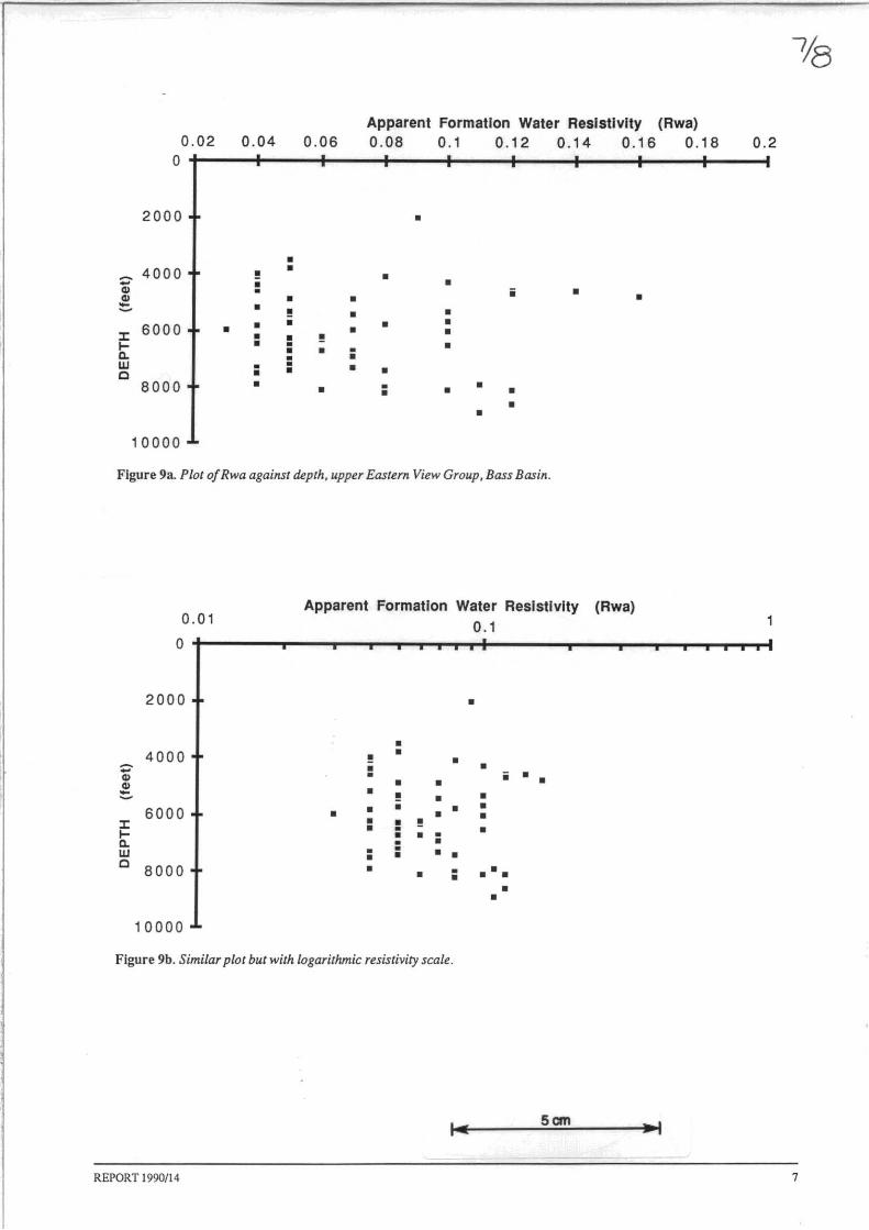
Figure 9a is a plot of apparent formation water resistivity (Rwa) against depth and Figure 9b is a similar plot, but using a logaritlunic scale for resistivity. Because hydrocarbons do not occur in the wells studied, Rwa is equivalent to true formation water resistivity (Rw). Most of the waters are fairly saline, with formation water salinities of between SO ()()() and 100 000 ppm NaCI equivalent, as determined from Schlumberger Chart Gen·' (Schlumberger, 1986).
From Figure 9 it is apparent that there is no obvious correlation between resistivity and depth, but the resistivities have been compared at the individual formation temperatures. As a general rule, there is an inverse relationship between resistivity and temperature (Helander, 1983), and so in a regional study such as this, the results should be normalised in some way to make any comparison meaningful.
The calculated resistivities were normalised to 7Sep using the equations below (derived from Asquith, 1982) - the [lISt equation determines temperature of the formation studied and the second calculates the resistivity at 7YP using the calculated formation temperature:-
T = [(TTO - TS)D T] o TD + S
Where:
TD = fonnation temperature at depth D; TTD = rrtaximum temperature recorded at Total Depth,
TO; TS = average surface temperature (taken as soep for
Bass Strait);
R _ Rwa (To + 6.77) 15 - (75 + 6.77)
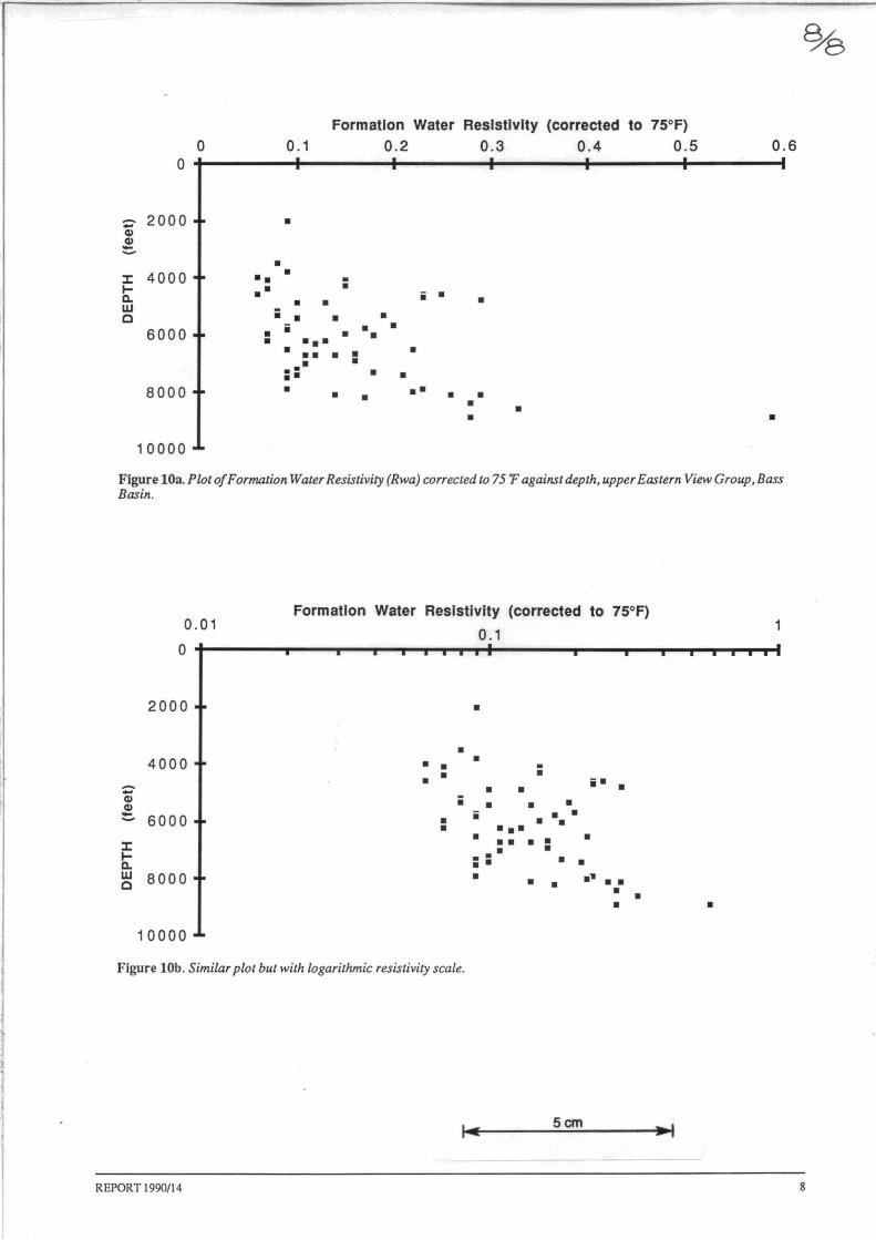
Figure lOa is a plot against depth of corrected resistivities and Figure lOb utilises a log scale for resistivity, similar to Figure 9b- at a constant temperature, the corrected resistivities may be regarded as a simple function of salinity. From Figure 10 it is now apparent qtat there is an increase of salinity with increase in depth (R = 0.21).
DISCUSSION
There are few published studies of variations in resistivity or salinity throughout a sedimentary basin. In many well-explored basins, water resistivity data have been compiled and published by numerous sources, but this data is mainly used for log evaluation purposes. Although no data or references were supplied, Helander (\983) notes that salinity and temperature generally increase with depth.
Production testing of the Pelican-5 well (fig. I) by Amoco Australia Petroleum Company in 1986 showed the presence of freshwater in Paleocene sands immediately underlying
REPORT 1990/1 4
very saline Eocene sands. Freshwater influx has been documented from the offshore Gippsland Basin, where a freshwater wedge infiltrates the upper Latrobe Group sediments in the northern and western parts of the basin (Kuuan et al., 1986). The freshwater is thoughllo be meteoric water which entered the Latrobe Group via an uplifted and exposed area of the onshore extension of the basin.
The present study, based on limited data, has indicated that there is a pattern of decrease in salinity towards the Paleocene section of the Bass Basin. As the Bass Basin sequences do not extend onshore, it is unlikely that freshwater flushing occurs, as is the case in the Gippsland Basin.
The change therefore is probably related to a fundamental geological factor. Brown (1976) notes that the lower Eastern View Group (i.e. lower Eocene and Paleocene) is predominantly shaly, whereas the upper Eastern View Group is more arenaceous. Baillie and Bacon (1989) described a regionally-occuring transgressive sand at the top of the Eastern View Group in the northern sector of the basin. It is possible that the apparent increase in salinity up through the Eocene section corresponds to this overall increase in the sand I shale ratio.
The present study has demonstrated the usefulness of the MacLog® software, and it is proposed to extend the present study to Paleocene and Cretaceous sections of the basin.
REFERENCES
ASQumt, G. B. 1982. Basic well log analysis for geologists. AAPG Methods in Exploration Series: Tulsa, Oklahoma USA.
BAILLIE, P. W.; BACON, C. A. 1989. Integrated sedimentological analysis: The Eocene of the Bass Basin. APEA J. 29(1): 312-327.
BoWLER, J. 1987. Why the Macintosh? A case study. Geobyte November 1987:48-53.
BROWN, B. R. 1976. Bass Basin, some aspects of the petroleum geology, in: LESUE, R. B.; EVANS, H. J.; KNIGlIT, C. L. (ed.). Economic Geology of Australia and Papua New Guinea, 3, Petroleum. M"""gr. Ser. Aust.lnst. Min. Metall. 7:67-82.
HELANDER, O. P. 1983. Fundamentals off ormation evaluation. OGCI Publications: Tulsa.
KtnTAN, K.; KUll.A, J. B.; NEUMANN, R. G. 1986. Freshwater influx in the GippslandBasin: impact on formation evaluation, hydrocarbon volumes and hydrocarbon migration. APEA J. 26(1):242-249.
NtCHOLAS, E.; l.ocKwOOD, K. L.; MARTIN, A. R.; JACKSON, K. S. 1981. Petroleum potential of the Bass Basin. J. Geol. Geophys Bur. Miner. Res. Aust. 6:199-212.
ROBINSON, V. A. 1974. Geological history of the Bass Basin. APEAJ.14:44-49.
SCHLUMBERGER. 1986. Log interpretation charts. Schlumberger Wen Services: USA.
SMITH, G . C. 1986. Bass Basin geology and petroleum exploration. in: GLENIE, R. C. (ed.). Second South· Eastern Australia Oil Exploration Symposium. 257-284.
WIlllAMSON, P. E.; PIGRAM, C. J.; COLWELL, J. B.; SCHER!., A. S.; l.ocKwooD, K. L.; BRANSON, J. C. 1985. Pre-Eocene stratigraphy, structure, and petroleum potential of the Bass Basin. APEA J. 25(1):362-381.
WIlllAMSON, P. E.; PIGRAM, C. J.; COLWELL, J. B.; SCHER!., A. S.; l.ocKwooD, K. L.; BRANSON, J. C. 1987. Review of stratigraphy, structure, and hydrocarbon potential of Bass Basin, Australia. AAPG Bull. 71:253-280.