35
Formulation of Circuit Equations Lecture 2 Alessandra Nardi Thanks to Prof. Sangiovanni-Vincentelli and Prof. Newton
| Date post: | 01-Jan-2016 |
| Category: |
Documents |
| Upload: | deirdre-morrison |
| View: | 225 times |
| Download: | 1 times |

Formulation of Circuit Equations
Lecture 2
Alessandra Nardi
Thanks to Prof. Sangiovanni-Vincentelli and Prof. Newton

219A: Course Overview
• Fundamentals of Circuit Simulation – Approximately 12 lectures
• Analog Circuits Simulation – Approximately 4 lectures
• Digital Systems Verification – Approximately 3 lectures
• Physical Issues Verification – Approximately 6 lectures
E.g.: SPICE, HSPICE,
PSPICE, SPECTRE, ELDO ….

SPICE historyProf. Pederson with “a cast of thousands”
• 1969-70: Prof. Roher and a class project– CANCER: Computer Analysis of Nonlinear Circuits, Excluding Radiation
• 1970-72: Prof. Roher and Nagel– Develop CANCER into a truly public-domain, general-purpose circuit simulator
• 1972: SPICE I released as public domain– SPICE: Simulation Program with Integrated Circuit Emphasis
• 1975: Cohen following Nagel research– SPICE 2A released as public domain
• 1976 SPICE 2D New MOS Models• 1979 SPICE 2E Device Levels (R. Newton appears)• 1980 SPICE 2G Pivoting (ASV appears)

Circuit Simulation
Simulator:Solve dx/dt=f(x) numerically
Input and setup Circuit
Output
Types of analysis:– DC Analysis– DC Transfer curves– Transient Analysis– AC Analysis, Noise, Distorsion, Sensitivity

Program Structure (a closer look)
Numerical Techniques:– Formulation of circuit equations
– Solution of linear equations
– Solution of nonlinear equations
– Solution of ordinary differential equations
Input and setup Models
Output

Formulation of Circuit Equations
Circuit withB branches
N nodes
Simulator
Set ofequations
Set ofunknowns

Formulation of Circuit Equations
• Unknowns– B branch currents (i)– N node voltages (e)– B branch voltages (v)
• Equations– N+B Conservation Laws – B Constitutive Equations

Branch Constitutive Equations (BCE)
• Determined by the mathematical model of the electrical behavior of a component– Example: V=R·I
• In most of circuit simulators this mathematical model is expressed in terms of ideal elements
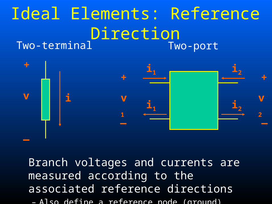
Ideal Elements: Reference Direction
Branch voltages and currents are measured according to the associated reference directions– Also define a reference node (ground)
+
_
v i
Two-terminal
+
_
v1
i1
Two-port
i1
+
_
v2
i2
i2

Branch Constitutive Equations (BCE)
Ideal elementsElement Branch Eqn
Resistor v = R·i
Capacitor i = C·dv/dt
Inductor v = L·di/dt
Voltage Source v = vs, i = ?
Current Source i = is, v = ?
VCVS vs = AV · vc, i = ?
VCCS is = GT · vc, v = ?
CCVS vs = RT · ic, i = ?
CCCS is = AI · ic, v = ?
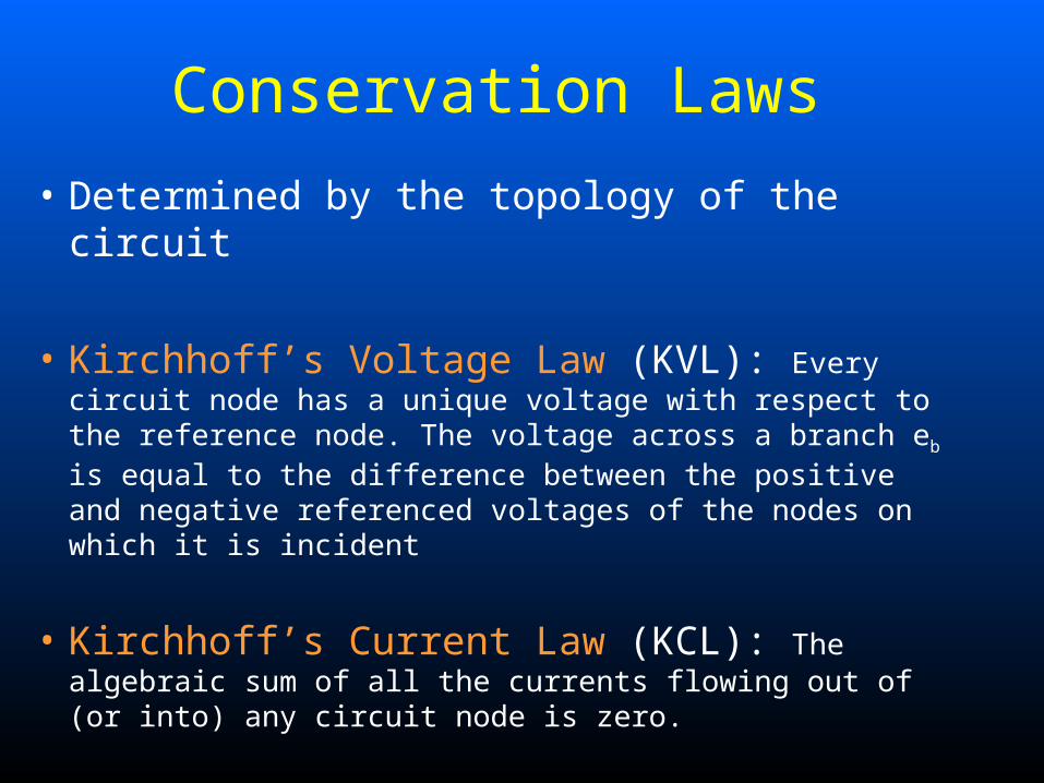
Conservation Laws
• Determined by the topology of the circuit
• Kirchhoff’s Voltage Law (KVL): Every circuit node has a unique voltage with respect to the reference node. The voltage across a branch eb is equal to the difference between the positive and negative referenced voltages of the nodes on which it is incident
• Kirchhoff’s Current Law (KCL): The algebraic sum of all the currents flowing out of (or into) any circuit node is zero.
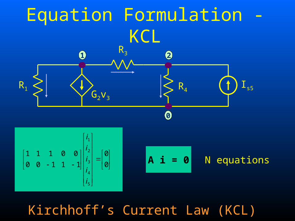
Equation Formulation - KCL
0
1 2
R1G2v3
R3
R4Is5
0
0
11100
00111
5
4
3
2
1
i
i
i
i
i
A i = 0
Kirchhoff’s Current Law (KCL)
N equations

Equation Formulation - KVL
0
1 2
R1G2v3
R3
R4Is5
0
0
0
0
0
10
10
11
01
01
2
1
5
4
3
2
1
e
e
v
v
v
v
v
v - AT e = 0
Kirchhoff’s Voltage Law (KVL)
B equations

Equation Formulation - BCE
0
1 2
R1G2v3
R3
R4Is5
55
4
3
2
1
5
4
3
2
1
4
3
2
1
0
0
0
0
00000
01
000
001
00
0000
00001
sii
i
i
i
i
v
v
v
v
v
R
R
GR
Kvv + i = is B equations

Equation FormulationNode-Branch Incidence Matrix
1 2 3 j B
12
i
N
branches
nodes (+1, -1, 0)
{Aij = +1 if node i is terminal + of branch j-1 if node i is terminal - of branch j0 if node i is not connected to branch j
PROPERTIES•A is unimodular•2 nonzero entries in each column

Equation Assembly (Stamping Procedures)
• Different ways of combining Conservation Laws and Constitutive Equations– Sparse Table Analysis (STA)
• Brayton, Gustavson, Hachtel
– Modified Nodal Analysis (MNA)• McCalla, Nagel, Roher, Ruehli, Ho

Sparse Tableau Analysis (STA)
1. Write KCL: Ai=0 (N eqns)
2. Write KVL: v -ATe=0 (B eqns)
3. Write BCE: Kii + Kvv=S (B eqns)
Se
v
i
KK
AI
A
vi
T 0
0
0
0
00N+2B eqnsN+2B unknowns
N = # nodesB = # branches
Sparse Tableau

Sparse Tableau Analysis (STA)
Advantages• It can be applied to any circuit• Eqns can be assembled directly from input
data• Coefficient Matrix is very sparse
ProblemSophisticated programming techniques and datastructures are required for time and memoryefficiency

Nodal Analysis (NA)
1. Write KCL
A·i=0 (N eqns, B unknowns)
2. Use BCE to relate branch currents to branch voltages
i=f(v) (B unknowns B unknowns)
3. Use KVL to relate branch voltages to node voltages
4. v=h(e) (B unknowns N unknowns)
Yne=ins
N eqnsN unknowns
N = # nodesNodal Matrix

Nodal Analysis - ExampleR3
0
1 2
R1G2v3
R4Is5
1. KCL: Ai=02. BCE: Kvv + i = is i = is - Kvv A Kvv = A is
3. KVL: v = ATe A KvATe = A is
Yne = ins
52
1
433
32
32
10
111
111
sie
e
RRR
RG
RG
R

Nodal Analysis
• Example shows NA may be derived from STA
• Better: Yn may be obtained by direct inspection (stamping procedure)– Each element has an associated stamp
– Yn is the composition of all the elements’ stamps

Spice input format: Rk N+ N- Rkvalue
Nodal Analysis – Resistor “Stamp”
kk
kk
RR
RR11
11N+ N-
N+
N-
N+
N-
iRk
sNNk
others
sNNk
others
ieeR
i
ieeR
i
1
1KCL at node N+
KCL at node N-
What if a resistor is connected to ground?
….Only contributes to the
diagonal
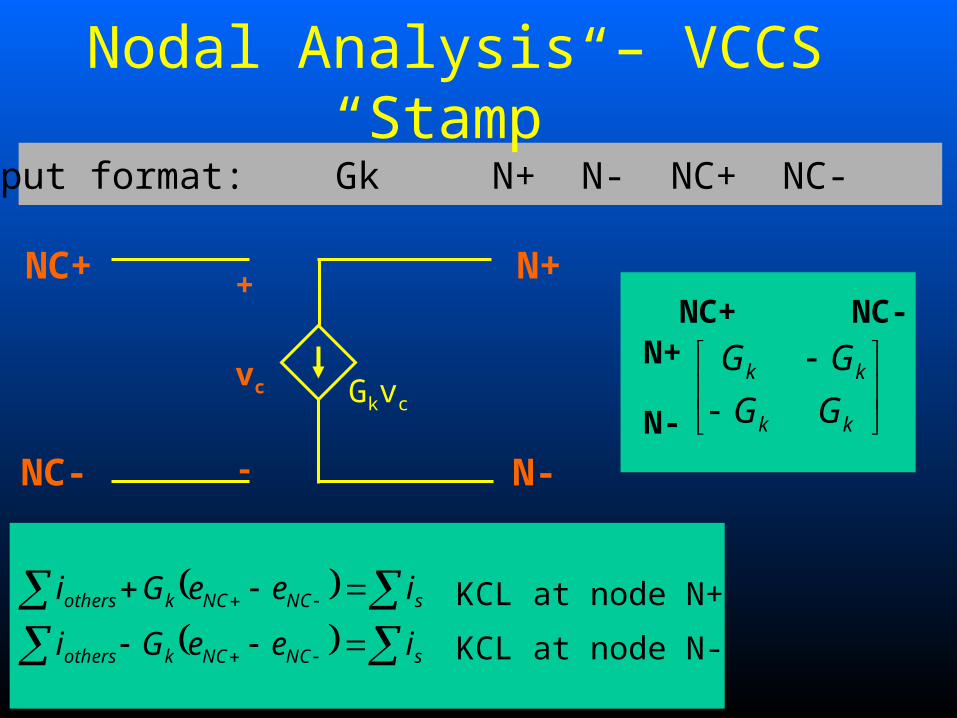
Spice input format: Gk N+ N- NC+ NC- Gkvalue
Nodal Analysis – VCCS “Stamp”
kk
kk
GG
GGNC+ NC-
N+
N-
N+
N-
Gkvc
NC+
NC-
+
vc
-
sNCNCkothers
sNCNCkothers
ieeGi
ieeGi KCL at node N+
KCL at node N-

Spice input format: Ik N+ N- Ikvalue
Nodal Analysis – Current source “Stamp”
k
k
I
IN+ N-
N+
N-
N+
N-
Ik
Nodal Analysis (NA)
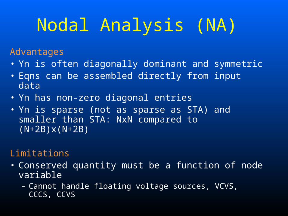
Advantages• Yn is often diagonally dominant and symmetric• Eqns can be assembled directly from input data• Yn has non-zero diagonal entries• Yn is sparse (not as sparse as STA) and smaller than
STA: NxN compared to (N+2B)x(N+2B)
Limitations• Conserved quantity must be a function of node variable
– Cannot handle floating voltage sources, VCVS, CCCS, CCVS

Modified Nodal Analysis (MNA)
• ikl cannot be explicitly expressed in terms of node voltages it has to be added as unknown (new column)
• ek and el are not independent variables anymore a constraint has to be added (new row)
How do we deal with independent voltage sources?
ikl
k l
+ -Ekl
klkl
l
k
Ei
e
e
011
1
1k
l

MNA – Voltage Source “Stamp”
ik
N+ N-
+ -Ek
Spice input format: ESk N+ N- Ekvalue
kE
0
00 0 1
0 0 -1
1 -1 0
N+
N-
Branch k
N+ N- ik RHS

Modified Nodal Analysis (MNA)
How do we deal with independent voltage sources?
Augmented nodal matrix
MSi
e
C
BYn
0
Some branch currents
MSi
e
DC
BYn
In general:

MNA – General rules
• A branch current is always introduced as and additional variable for a voltage source or an inductor
• For current sources, resistors, conductors and capacitors, the branch current is introduced only if:– Any circuit element depends on that branch current– That branch current is requested as output

MNA – CCCS and CCVS “Stamp”

MNA – An example
Step 1: Write KCLi1 + i2 + i3 = 0 (1)-i3 + i4 - i5 - i6 = 0 (2)i6 + i8 = 0 (3)i7 – i8 = 0 (4)
0
1 2
G2v3
R4Is5R1
ES6- +
R8
3
E7v3
- +4

MNA – An exampleStep 2: Use branch equations to eliminate as many branch currents as possible1/R1·v1 + G2 ·v3 + 1/R3·v3 = 0 (1)- 1/R3·v3 + 1/R4·v4 - i6 = is5
(2)i6 + 1/R8·v8 = 0 (3)i7 – 1/R8·v8 = 0 (4)
Step 3: Write down unused branch equationsv6 = ES6 (b6)v7 – E7·v3 = 0
(b7)

MNA – An exampleStep 4: Use KVL to eliminate branch voltages from previous equations1/R1·e1 + G2·(e1-e2) + 1/R3·(e1-e2) = 0 (1)- 1/R3·(e1-e2) + 1/R4·e2 - i6 = is5 (2)i6 + 1/R8·(e3-e4) = 0 (3)i7 – 1/R8·(e3-e4) = 0 (4)(e3-e2) = ES6 (b6)e4 – E7·(e1-e2) = 0 (b7)
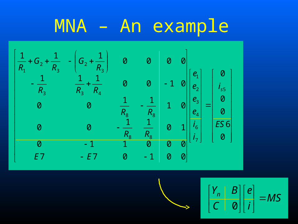
MNA – An example
0
6
0
0
0
001077
000110
1011
00
0111
00
0100111
0000111
5
7
6
4
3
2
1
88
88
433
32
32
1
ES
i
i
i
e
e
e
e
EE
RR
RR
RRR
RG
RG
R
s
MSi
e
C
BYn
0

Modified Nodal Analysis (MNA)
Advantages• MNA can be applied to any circuit• Eqns can be assembled directly from input
data• MNA matrix is close to Yn
Limitations• Sometimes we have zeros on the main
diagonal and principle minors may also be singular.


![[Malik et al 1988] Malik, S., Wang, A., Brayton, R. K ... › ~bryant › pubdir › CMU-CS-92-160.pdf[Malik et al 1988] Malik, S., Wang, A., Brayton, R. K., and Sangiovanni-Vincentelli,](https://static.documents.pub/doc/80x56/5f0cd6787e708231d437611b/malik-et-al-1988-malik-s-wang-a-brayton-r-k-a-bryant-a-pubdir.jpg)


