Foundation Engineering Dr. Priti Maheshwari Department Of Civil Engineering Indian Institute Of Technology, Roorkee Module - 02 Lecture - 05 Lateral Earth Pressure Theories and Retaining Walls - 5 Good afternoon, in the last class, we were discussing about the check for bearing capacity failure, that is how you can find out the factor of safety against bearing capacity failure. In that respect, we found out that, what will be the q maximum and q minimum at the base of the wall that is base slab. So, let us try to see, some of the points that you should take into account, while you carry out further analysis in case of bearing capacity failure. (Refer Slide Time: 01:02) You must always remember that summation V, which was there in that particular table, as I explained you in the last class, it includes the soil weight also. Now, we have found out the value of eccentricity, when this value of eccentricity becomes more than B by 6. In that case, your q minimum becomes negative and as soon as, that q becomes negative, it indicates the development of tensile stress at the end of heel section. Q minimum is occurring at heel, if this q minimum is negative, that gives the development of tensile stress.
Transcript
Foundation Engineering
Dr. Priti Maheshwari
Department Of Civil Engineering
Indian Institute Of Technology, Roorkee
Module - 02
Lecture - 05
Lateral Earth Pressure Theories and Retaining Walls - 5
Good afternoon, in the last class, we were discussing about the check for bearing
capacity failure, that is how you can find out the factor of safety against bearing capacity
failure. In that respect, we found out that, what will be the q maximum and q minimum
at the base of the wall that is base slab. So, let us try to see, some of the points that you
should take into account, while you carry out further analysis in case of bearing capacity
failure.
(Refer Slide Time: 01:02)
You must always remember that summation V, which was there in that particular table,
as I explained you in the last class, it includes the soil weight also. Now, we have found
out the value of eccentricity, when this value of eccentricity becomes more than B by 6.
In that case, your q minimum becomes negative and as soon as, that q becomes negative,
it indicates the development of tensile stress at the end of heel section. Q minimum is
occurring at heel, if this q minimum is negative, that gives the development of tensile
stress.
This stress is not at all desirable, because the tensile strength of the soil is, very, very
small. So, you we must avoid, this kind of situation, so in any case, the eccentricity
should not be greater than B by 6, where B is the width of based slab.
(Refer Slide Time: 02:11)
Now, what happens if, in the analysis by analysing the procedure, this e comes out be
more than B by 6, then in that case, the design should be re-proportioned and calculation
should be redone. So, let us say that, you took a tentative proportioning of the wall, you
carried out the analysis, it worked out to be safe against overturning, it worked out to be
safe against sliding along the base. And then, while you working, while you were
working out, the factor of safety against bearing capacity failure.
And in that process, if you, if the eccentricity of the force comes out to be more than B
by 6, immediately you should stop the analysis, at that particular point of time and you
should re-proportion the whole thing and do the calculation altogether again. Because,
development of any tensile stress is not at all desirable, in case of soil. Then, in the
shallow foundation chapter, you already have studied, that how you can find out the
ultimate bearing capacity of the foundation, which is I am giving you for the reference
purpose, that this way you can find out your q u.
So, q u is equal to c 2 N c F c d F c i plus q N q F q d F q i plus half gamma 2 B time N
gamma F gamma d F gamma i. Now, let us try to see, what are the different terms in this
particular expression.
(Refer Slide Time: 03:46)
Q is gamma 2 into D, B prime is B minus 2 e, e is the eccentricity, that you have to
obtain as explained earlier. F c d, F q d and F gamma d, they are the standard expressions
given by Terzaghi or different other research workers, you can simply pick the standard
values by using these expression, for these. And F c i, F q i, F gamma i, they are the
function of this angle psi, which can be obtained by this particular expression, that is tan
inverse P a cos of alpha by summation of V.
(Refer Slide Time: 04:27)
So, once the, ultimate bearing capacity of the soil has been calculated, the factor of
safety against bearing capacity failure, can be obtained as, factor of safety bearing
capacity is equal to q u by q max. So, this q u, we are calculating using the expression,
either by, given by Terzaghi or any other expression, given by any other research worker
and then, this q max, you have already found out, you remember that, you found out the
q max and q minimum.
So, from there, whatever is the maximum value of q, you simply divide q u by that and
then, you will be getting this factor of safety against bearing capacity. Generally, a factor
of safety of 3 is required, in this case, that is against bearing capacity failure; the ultimate
bearing capacity of shallow foundations occur, at a settlement of about 10% of
foundation width, so that, this aspect also we must take in to account.
(Refer Slide Time: 05:28)
Now, in case of retaining walls, the width B is large and hence, the ultimate load, q u
will occur at fairly large foundation settlement and the factor of safety of 3, against
bearing capacity failure may not ensure, that the settlement will be within tolerable limit.
So, this aspect, we should always keep in our mind and we should have the provision of
further investigation, as for as, this aspect is concerned. As, it is beyond the scope of this
course, so I am not discussing all these things in detail,
But you must always remember this thing, that although the wall is safe against the three
aspects, that is over turning, sliding and bearing capacity failure. However, due to the
large or excessive settlement, the service ability criteria is not satisfied, so in that
condition, we need to take the proper care.
(Refer Slide Time: 06:30)
Now, this was all the theoretical part, that we discussed, now let us try to take an
example, so that, that will give you the feel, that how you can find out the both, factor of
safety against overturning, the factor of safety against sliding along the base of the wall
and the factor of safety against bearing capacity failure, so we will take up an example.
The cross section of a cantilever wall is shown in this figure below, calculate the factors
of safety with respect to overturning, sliding and the bearing capacity.
This is the statement of the, this example, that I am going to solve here, you can see here,
that this is a wall incline back field, which is having an inclination of 10 degree from the
horizontal. This soil is frictionless, c 1 is equal to 0, it is having an angle of internal
friction as 30 degree, the unit weight of this backfill soil is 18 kilonewton per meter
cube, here it is 20 degree and 40 kilonewton per meter square, c 2 value, gamma 2 value
is 19 kilonewton per meter cube, that is the soil, which is lying below the basal slab is
having these properties.
Then, the soil is placed at a depth of 1.5 meter below the ground surface, this, the
tentative dimension, that has been taken here is that, the thickness of the basal slab is 0.7
meter, this height, from this particular point, that is base of the wall up to this much is 6
meters, then here, the part of this heel slab, that is the width of this heel slab is 2.6 meter.
For this one, it is like the thickness of the stem at the base is 0.7 meter and this
dimension is also 1.7 meter.
Then, since it is inclined and we have seen, that this active force will be acting parallel to
this inclined face, so you see, this is the P a, that is the direction of the, this active force
which is acting on the wall, it has been assumed, that the failure is taking place along this
vertical face, it is component, horizontal component is P h, vertical component is P v.
Then, this whole area has been divided, that is the weight of the soil is being represented
by this area 4 and this, by area 5.
However, the weight of the wall is being divided into three sections, that is section 1,
section 2, this is small triangular area and this section 3, which is the area of the base
slab.
(Refer Slide Time: 09:34)
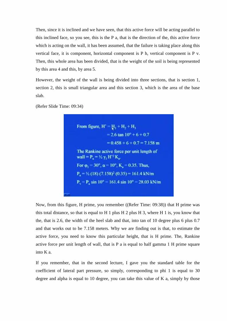
Now, from this figure, H prime, you remember ((Refer Time: 09:38)) that H prime was
this total distance, so that is equal to H 1 plus H 2 plus H 3, where H 1 is, you know that
the, that is 2.6, the width of the heel slab and that, into tan of 10 degree plus 6 plus 0.7
and that works out to be 7.158 meters. Why we are finding out is that, to estimate the
active force, you need to know this particular height, that is H prime. The, Rankine
active force per unit length of wall, that is P a is equal to half gamma 1 H prime square
into K a.
If you remember, that in the second lecture, I gave you the standard table for the
coefficient of lateral part pressure, so simply, corresponding to phi 1 is equal to 30
degree and alpha is equal to 10 degree, you can take this value of K a, simply by those
standard table, so Ka works out to be 0.35. Thus, from this expression, if we substitute
all the values, your P a works out to be 161.4 kilonewton per meter.
Then, vertical component of this particular active force is equal to P a sin of 10 degree,
that works out to be 28.03 kilonewton per meter.
(Refer Slide Time: 11:05)
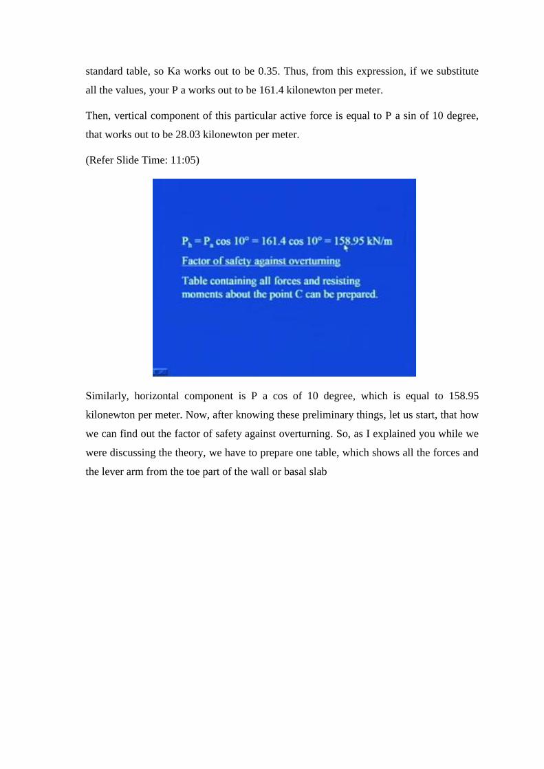
Similarly, horizontal component is P a cos of 10 degree, which is equal to 158.95
kilonewton per meter. Now, after knowing these preliminary things, let us start, that how
we can find out the factor of safety against overturning. So, as I explained you while we
were discussing the theory, we have to prepare one table, which shows all the forces and
the lever arm from the toe part of the wall or basal slab
(Refer Slide Time: 11:39)
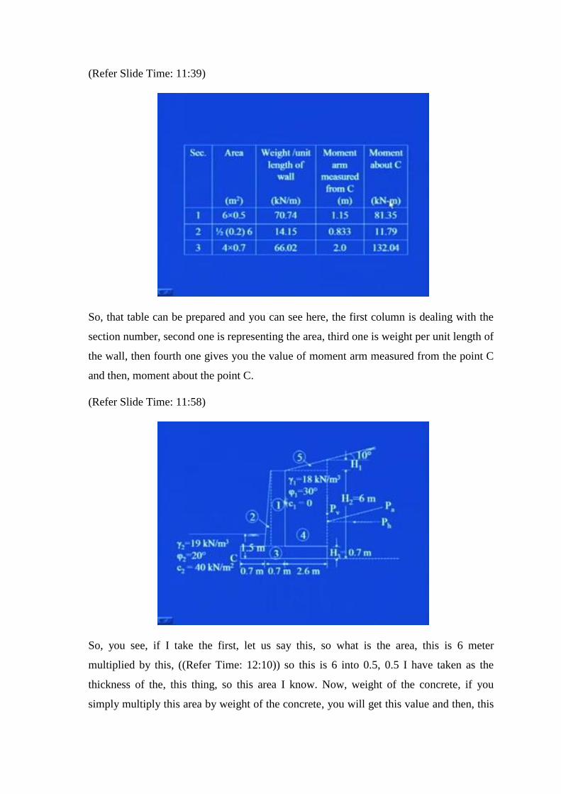
So, that table can be prepared and you can see here, the first column is dealing with the
section number, second one is representing the area, third one is weight per unit length of
the wall, then fourth one gives you the value of moment arm measured from the point C
and then, moment about the point C.
(Refer Slide Time: 11:58)
So, you see, if I take the first, let us say this, so what is the area, this is 6 meter
multiplied by this, ((Refer Time: 12:10)) so this is 6 into 0.5, 0.5 I have taken as the
thickness of the, this thing, so this area I know. Now, weight of the concrete, if you
simply multiply this area by weight of the concrete, you will get this value and then, this
is acting, you see if it is, this is 0.5, so this is half of this is 0.75. So, then you add this
distance to this 0.75, you will be getting, sorry 0.25.
You will be getting the lever arm from this point C, so that is 1.15, you simply multiply
this weight per unit length of the wall by this moment arm, this will give you the moment
about the point C, due to the sectional area 1. Likewise, this sectional area 2, which is
this small triangular part, you simply find out the area of this particular one, that is half
0.2 into 6 and then weight, simply multiplied by unit weight of the concrete, in this area
and you will be getting this weight per unit length of the wall.
Then, the momentum, you can find out, it is 0.833 in this case, you multiply, this weight
per unit length of the wall by this momentum, you will be getting this moment about C.
Similarly, for the third one, see this is 2.6 plus 0.7 plus 0.7 that is 4, multiply by 0.7, this
will give you the area. You multiply by gamma of concrete, you will be getting weight
per unit length of the wall, due to this sectional area 3 and this will be acting at a distance
of 2 meter.
You see here, this momentum is 2 meter, simply multiply by those two values and you
will be getting the moment about the point C.
(Refer Slide Time: 14:08)
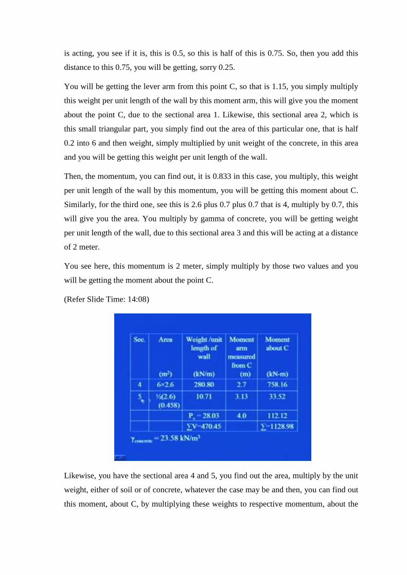
Likewise, you have the sectional area 4 and 5, you find out the area, multiply by the unit
weight, either of soil or of concrete, whatever the case may be and then, you can find out
this moment, about C, by multiplying these weights to respective momentum, about the
point C. In this problem, I have taken this gamma, concrete to be equal to 23.58
kilonewton per meter cube.
Then, this P v, we have found out, that is the vertical component of active force, which
was out to be 28.03 kilonewton per meter and this will be acting at a lever arm of equal
to base width of the slab, which is 4 meter in our case, multiply by these, multiply these
two values and you will be getting here, this moment about C, due to this vertical
component of active force. You simply add, all the values, that is the value of weight of
wall per unit length of the wall, for section 1, 2 , 3, 4 and 5.
And then, this particular P v, you will result in to this amount, that is 470.45 kilonewton
per meter is the total vertical force, which is acting on the wall, due to the weight of wall,
due to the weight of soil, which is lying above the heel and due to the vertical component
of active force and then you take the summation of all the moments, that is, in this
particular column, that moment about the point C, that will result into 1128.98
kilonewton per meter, that is the total resisting moment.
Once this table is complete, now the rest part becomes little simpler, for us.((Refer Time:
16:10)).So, you see here, for all the five sections, that is 1, 2, 3, 4 and 5, we found out the
width, by multiplying it is area to respective unit weight of soil or concrete, say for first
second and third section, we multiply the area by gamma of concrete, that is unit weight
of concrete can be found out the weight per unit length of the wall.
And then, for 4 and 5, we multiply by this gamma 1 that is, 18 kilonewton per meter
cube, to the respective areas to get the weight per unit length of the wall.
(Refer Slide Time: 16:46)
And then, the overturning moment, as you know that, the only overturning, the only
force which was causing the over turning, was the horizontal component of that active
force, which was P h and that was acting at a distance of H prime by 3 from the base of
the wall and it is magnitude, we found out as 158.95 H prime, we have already worked
out and this Mo works out to be 379.25 kilonewton per meter. You have already found
out summation M R, here we calculate it summation Mo.
So, how we can find out your factor of safety against overturning, is that, the ratio of
summation of all resisting moments, to the summation of all the moments, which are
causing the overturning, so you see here, 1128.98 divided by 379.25, which works out to
be 2.98 and I as, I told you, that for overturning, the factor of safety can be considered
between 2 to 3, so this is greater than 2, so the wall is safe against overturning.
So, the factor of, we have to find out the objective was, that we have to find out factor of
safety against overturning, factor of safety against sliding and factor of safety against
bearing capacity failure. So, here, we have found out the first part, which is factor of
safety against overturning and it worked out to be 2.98, which is greater than 2 and
hence, the wall is safe against overturning. Now, let us try to see, that how we can find
out the factor of safety against sliding.
(Refer Slide Time: 18:34)
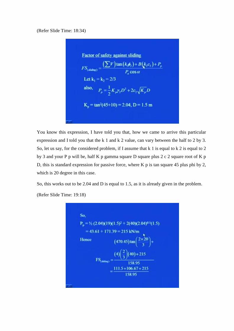
You know this expression, I have told you that, how we came to arrive this particular
expression and I told you that the k 1 and k 2 value, can vary between the half to 2 by 3.
So, let us say, for the considered problem, if I assume that k 1 is equal to k 2 is equal to 2
by 3 and your P p will be, half K p gamma square D square plus 2 c 2 square root of K p
D, this is standard expression for passive force, where K p is tan square 45 plus phi by 2,
which is 20 degree in this case.
So, this works out to be 2.04 and D is equal to 1.5, as it is already given in the problem.
(Refer Slide Time: 19:18)
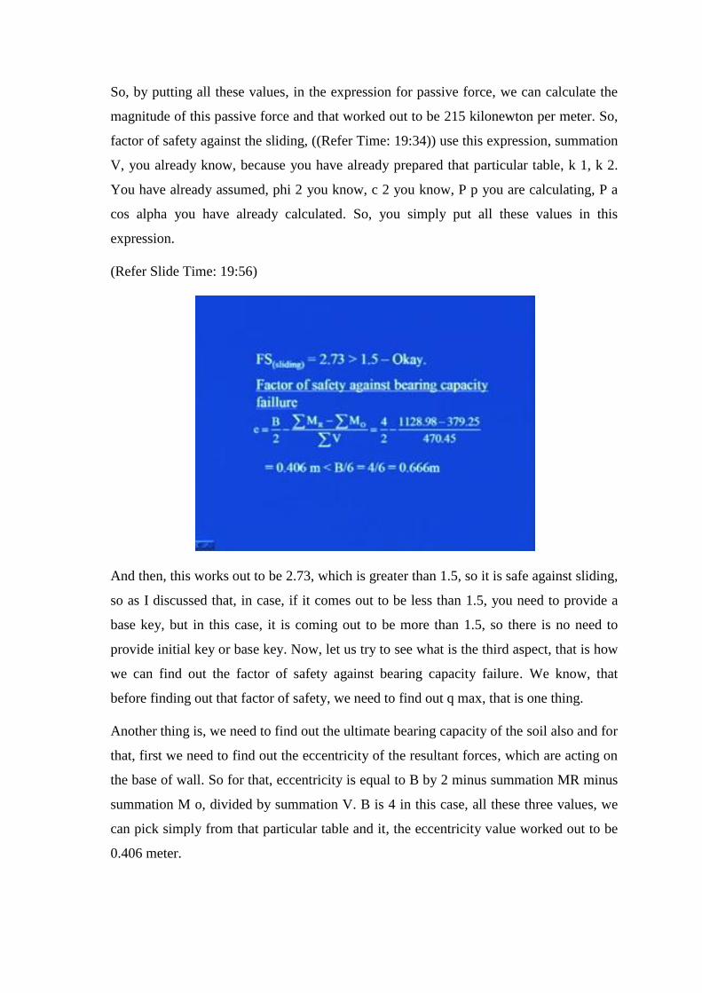
So, by putting all these values, in the expression for passive force, we can calculate the
magnitude of this passive force and that worked out to be 215 kilonewton per meter. So,
factor of safety against the sliding, ((Refer Time: 19:34)) use this expression, summation
V, you already know, because you have already prepared that particular table, k 1, k 2.
You have already assumed, phi 2 you know, c 2 you know, P p you are calculating, P a
cos alpha you have already calculated. So, you simply put all these values in this
expression.
(Refer Slide Time: 19:56)
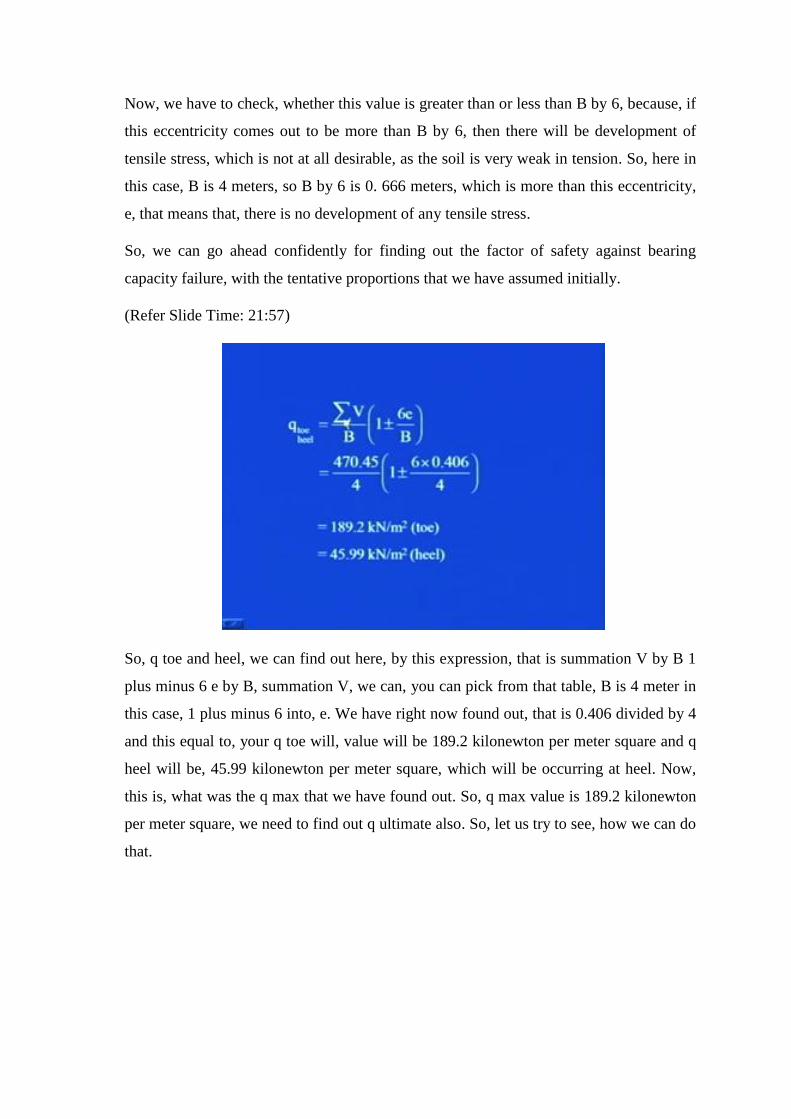
And then, this works out to be 2.73, which is greater than 1.5, so it is safe against sliding,
so as I discussed that, in case, if it comes out to be less than 1.5, you need to provide a
base key, but in this case, it is coming out to be more than 1.5, so there is no need to
provide initial key or base key. Now, let us try to see what is the third aspect, that is how
we can find out the factor of safety against bearing capacity failure. We know, that
before finding out that factor of safety, we need to find out q max, that is one thing.
Another thing is, we need to find out the ultimate bearing capacity of the soil also and for
that, first we need to find out the eccentricity of the resultant forces, which are acting on
the base of wall. So for that, eccentricity is equal to B by 2 minus summation MR minus
summation M o, divided by summation V. B is 4 in this case, all these three values, we
can pick simply from that particular table and it, the eccentricity value worked out to be
0.406 meter.
Now, we have to check, whether this value is greater than or less than B by 6, because, if
this eccentricity comes out to be more than B by 6, then there will be development of
tensile stress, which is not at all desirable, as the soil is very weak in tension. So, here in
this case, B is 4 meters, so B by 6 is 0. 666 meters, which is more than this eccentricity,
e, that means that, there is no development of any tensile stress.
So, we can go ahead confidently for finding out the factor of safety against bearing
capacity failure, with the tentative proportions that we have assumed initially.
(Refer Slide Time: 21:57)
So, q toe and heel, we can find out here, by this expression, that is summation V by B 1
plus minus 6 e by B, summation V, we can, you can pick from that table, B is 4 meter in
this case, 1 plus minus 6 into, e. We have right now found out, that is 0.406 divided by 4
and this equal to, your q toe will, value will be 189.2 kilonewton per meter square and q
heel will be, 45.99 kilonewton per meter square, which will be occurring at heel. Now,
this is, what was the q max that we have found out. So, q max value is 189.2 kilonewton
per meter square, we need to find out q ultimate also. So, let us try to see, how we can do
that.
(Refer Slide Time: 22:52)
So, the ultimate capacity given by this standard equation, you know that, for different
values of phi, you have the standard tables, you can pick the safe factors accordingly,
sorry bearing capacity factors accordingly, which are N c, N q and N gamma. So, simply
these values have been picked from the standard table, q, which is coming here is gamma
2 into D, gamma 2 is 19 into 1.5, which works out to be 28.5 kilonewton per meter
square.
B prime is equal to B minus 2 e, e you have found out as 0.406 meter, B is 4 meter, so
that B prime works out to be 3.188 meter, then F c d, F q d.
(Refer Slide Time: 23:35)
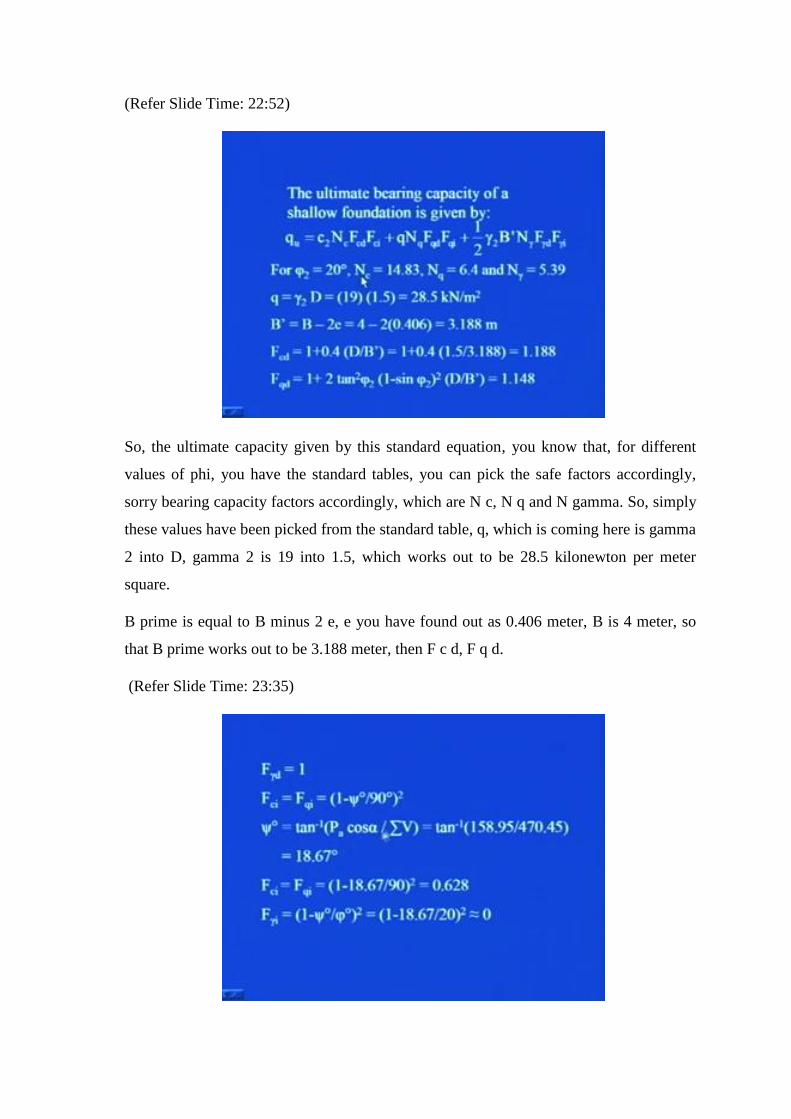
And F gamma d from standard expressions, similarly, F c i, F q i, you require psi degree
and that psi degree is define as tan inverse P a cos alpha by summation V, P a cos alpha
you know, summation V also you know, you can simply pick these values from the table,
that psi degree will become equal to 18.67 degree. Once this psi is known, you can find
out this F c i and F q i, so F c i and F q i, they worked out to be 0.628. However, F
gamma i, which is equal to 1 minus psi degree by phi degree whole square.
That is approximately very less value, so I am taking approximately that to be equal to 0.
(Refer Slide Time: 24:26)
So, q will become, similarly you have the expression, simply put all the values in that
expression and then, this q value will work out to be 574.07 kilonewton per meter
square. Please make, please note it that, since this F gamma i worked out to be 0, that is
why, this third term is coming out to be 0. If, it has some value, you simply put that value
and then you get the corresponding value of q, then factor of safety against bearing
capacity failure, it is equal to q u by q max, q max in this case is equal to q toe.
That you have already worked out and this works out to be 3.03, which is greater than 3,
so the wall is safe against bearing capacity failure also. So, I hope the procedure of
obtaining the factor of safety against overturning, the factor of safety against sliding
along the base, the factor of safety against bearing capacity failure is clear to you. That,
how you can implement all the theoretical things as we discussed in to any practical
problem. Now, this was all about the stability of the wall.
(Refer Slide Time: 25:46)
There are few points or comments, that we must know about the stability of the wall, so
let us try to discuss one by one, that what are those comments related to the stability. So,
when the weak soil layer is located at a shallow depth, that is, within a depth about 1.5
times the width of retaining wall, the bearing capacity of the weak layer should be
carefully investigated. As, you know that, wherever there is a presence of any weak soil
layer, we need to be extra careful.
So, that is what, this first comment tells us, that we need to be extra careful, for the
bearing capacity of weak layer. Then, we have not talked of anything related to the
settlement, but that is an important serviceability criteria, you must always keep in to
mind, that the possibility of excessive settlement also should be considered. It may
happen, that the wall is safe against overturning sliding and bearing capacity failure,
however, the settlement can be to quite high.
So, for that, that possibility we should always keep into our mind, the use of light weight
backfill material behind the wall, may solve stability problem. So, that also, is another
option.
(Refer Slide Time: 27:07)
Then, piles are used to transmit foundation load to the firmer layer, you will be studying
these piles, just for the time being, you can think of that, during your foundation chapter
you have studied for shallow foundation. Piles are kind of deep foundation, we will be
discussing them in some subsequent lectures, but for time being, you just simply think
that, it is a kind of deep foundation. However, often the thrust of the sliding wedge of the
soil, in case of deep shear failure, bends, it bends the pile and eventually causes them to
fail.
So, we need to keep into account, that when the piles are being used, that they should not
bend and should not fail, so careful attention should be given to this possibility when
considering the option of pile foundation for retaining walls. Then, the active earth
coefficient is used to determine the lateral force of the back fill, the active state of
backfill can be established only if wall yields sufficiently, which does not happen in all
the cases.
This aspect we have already discussed, that for any soil to enter in to either active state
or passive state, the wall must move or must yield sufficiently, so that those conditions
are generated. So, usually in all the cases, it is not generated, so we must take in to
account, that whether the active condition or the passive condition is really getting
generated or not. The degree of wall yielding will depend on its height and the section
modulus.
(Refer Slide Time: 28:50)
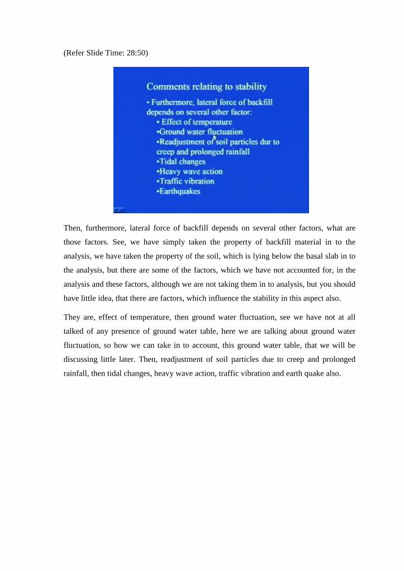
Then, furthermore, lateral force of backfill depends on several other factors, what are
those factors. See, we have simply taken the property of backfill material in to the
analysis, we have taken the property of the soil, which is lying below the basal slab in to
the analysis, but there are some of the factors, which we have not accounted for, in the
analysis and these factors, although we are not taking them in to analysis, but you should
have little idea, that there are factors, which influence the stability in this aspect also.
They are, effect of temperature, then ground water fluctuation, see we have not at all
talked of any presence of ground water table, here we are talking about ground water
fluctuation, so how we can take in to account, this ground water table, that we will be
discussing little later. Then, readjustment of soil particles due to creep and prolonged
rainfall, then tidal changes, heavy wave action, traffic vibration and earth quake also.
(Refer Slide Time: 30:04)
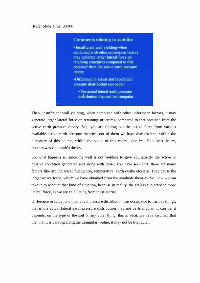
Then, insufficient wall yielding, when combined with other unforeseen factors, it may
generate larger lateral force on retaining structures, compared to that obtained from the
active earth pressure theory. See, you are finding out the active force from various
available active earth pressure theories, out of them we have discussed to, within the
periphery of this course, within the scope of this course, one was Rankine's theory,
another was Coulomb’s theory.
So, what happens is, since the wall is not yielding to give you exactly the active or
passive condition generated and along with those, you have seen that, there are many
factors like ground water fluctuation, temperature, earth quake etcetera. They cause the
larger active force, which we have obtained from the available theories. So, how we can
take in to account that kind of situation, because in reality, the wall is subjected to more
lateral force, as we are calculating from these stories.
Difference in actual and theoretical pressure distribution can occur, due to various things,
that is the actual lateral earth pressure distribution may not be triangular. It can be, it
depends, on the type of the soil or any other thing, this is what, we have assumed that
the, that it is varying along the triangular wedge, it may not be triangular.
(Refer Slide Time: 31:40)
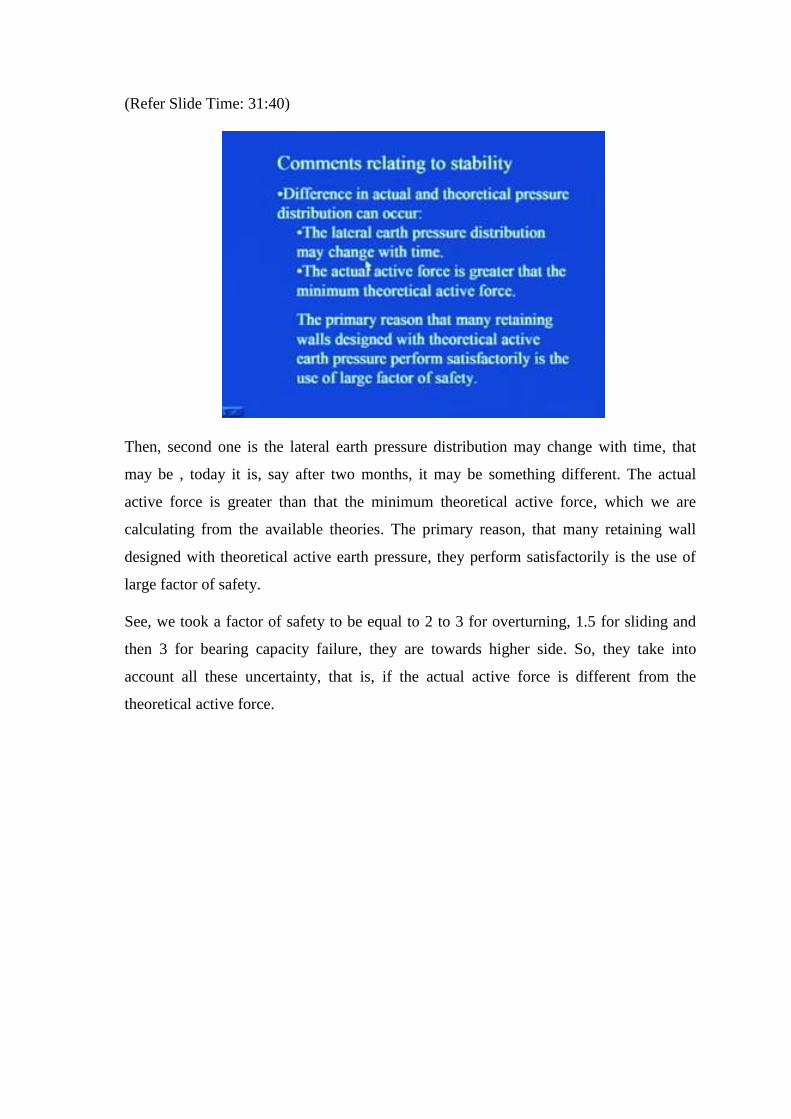
Then, second one is the lateral earth pressure distribution may change with time, that
may be , today it is, say after two months, it may be something different. The actual
active force is greater than that the minimum theoretical active force, which we are
calculating from the available theories. The primary reason, that many retaining wall
designed with theoretical active earth pressure, they perform satisfactorily is the use of
large factor of safety.
See, we took a factor of safety to be equal to 2 to 3 for overturning, 1.5 for sliding and
then 3 for bearing capacity failure, they are towards higher side. So, they take into
account all these uncertainty, that is, if the actual active force is different from the
theoretical active force.
(Refer Slide Time: 32:34)
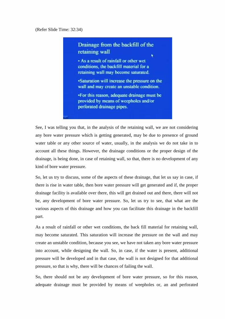
See, I was telling you that, in the analysis of the retaining wall, we are not considering
any bore water pressure which is getting generated, may be due to presence of ground
water table or any other source of water, usually, in the analysis we do not take in to
account all these things. However, the drainage conditions or the proper design of the
drainage, is being done, in case of retaining wall, so that, there is no development of any
kind of bore water pressure.
So, let us try to discuss, some of the aspects of these drainage, that let us say in case, if
there is rise in water table, then bore water pressure will get generated and if, the proper
drainage facility is available over there, this will get drained out and there, there will not
be, any development of bore water pressure. So, let us try to see, that what are the
various aspects of this drainage and how you can facilitate this drainage in the backfill
part.
As a result of rainfall or other wet conditions, the back fill material for retaining wall,
may become saturated. This saturation will increase the pressure on the wall and may
create an unstable condition, because you see, we have not taken any bore water pressure
into account, while designing the wall. So, in case, if the water is present, additional
pressure will be developed and in that case, the wall is not designed for that additional
pressure, so that is why, there will be chances of failing the wall.
So, there should not be any development of bore water pressure, so for this reason,
adequate drainage must be provided by means of weepholes or, an and perforated
drainage pipes. You can either use weepholes or you can use, perforated drainage pipes
or a combination of both.
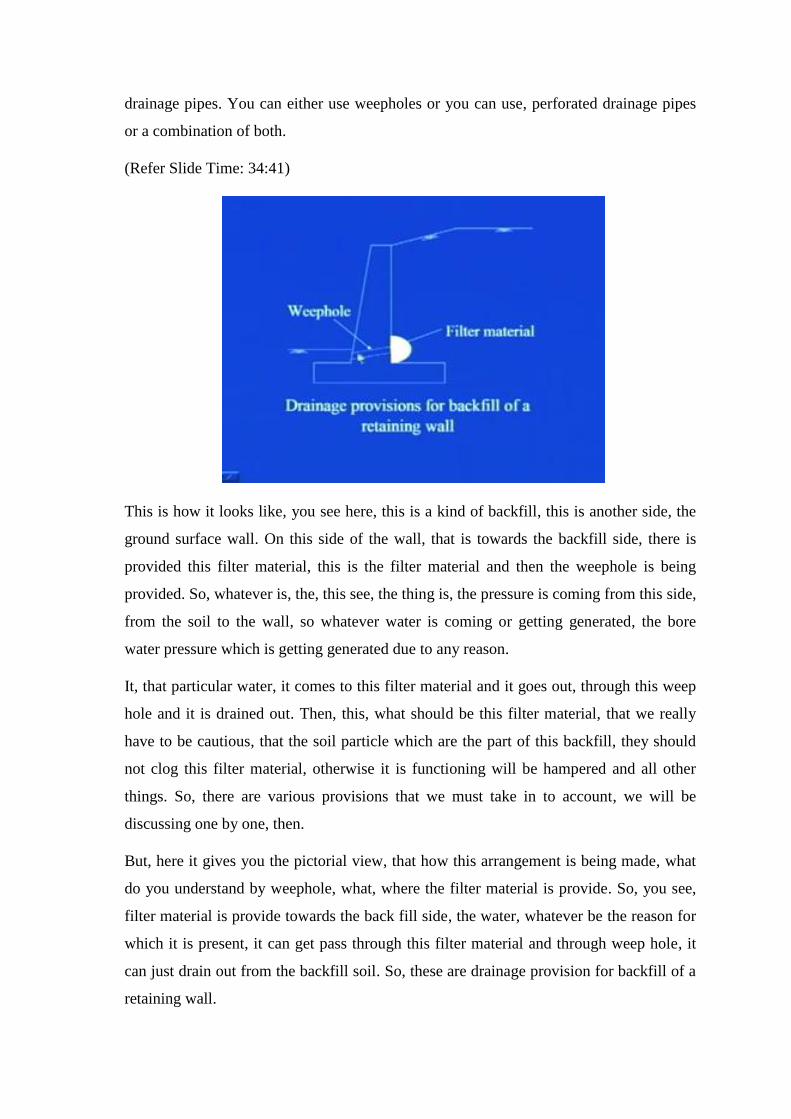
(Refer Slide Time: 34:41)
This is how it looks like, you see here, this is a kind of backfill, this is another side, the
ground surface wall. On this side of the wall, that is towards the backfill side, there is
provided this filter material, this is the filter material and then the weephole is being
provided. So, whatever is, the, this see, the thing is, the pressure is coming from this side,
from the soil to the wall, so whatever water is coming or getting generated, the bore
water pressure which is getting generated due to any reason.
It, that particular water, it comes to this filter material and it goes out, through this weep
hole and it is drained out. Then, this, what should be this filter material, that we really
have to be cautious, that the soil particle which are the part of this backfill, they should
not clog this filter material, otherwise it is functioning will be hampered and all other
things. So, there are various provisions that we must take in to account, we will be
discussing one by one, then.
But, here it gives you the pictorial view, that how this arrangement is being made, what
do you understand by weephole, what, where the filter material is provide. So, you see,
filter material is provide towards the back fill side, the water, whatever be the reason for
which it is present, it can get pass through this filter material and through weep hole, it
can just drain out from the backfill soil. So, these are drainage provision for backfill of a
retaining wall.
(Refer Slide Time: 36:27)
Then, weepholes, if provided, should have a minimum diameter of about 0.1 meter and
be adequately placed. You see, if it is having lesser diameter, what will happen, that it
may happen, that many a times soil particles from backfill, if they are also coming with
water and they may clog the weephole, which will result the insufficient drainage and
will cause the wall to become unstable. There is always a possibility, that the back fill
material may be washed into weep holes or drainage pipes and ultimately, clog them.
Thus, a filter material needs to be placed behind the weep holes or around the drainage
pipes. ((Refer Time: 37:10))You see, this, let us say the water is getting accumulated
here, it has to pass through this weephole, if this filter material is not here, what will
happen, that some of the clay particles or some of the soil particles will come, with the
water, they will come through this weephole and simply, some of them will pass through
the weephole and some of them will be remaining and over a period of time, they will
clog this weephole.
So, that is why, this filter material is provided over here, so that, the first filtering of the
water, from this backfill material is takes place at this particular stage only. So, many of
the soil particles, they get struck up here, they get filter out here and then only water goes
into this weep hole. So, that is what is that, the filter material is placed for that particular
reason.
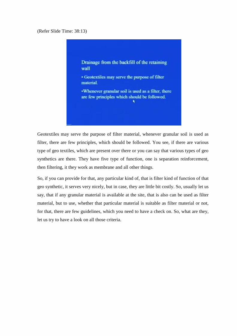
(Refer Slide Time: 38:13)
Geotextiles may serve the purpose of filter material, whenever granular soil is used as
filter, there are few principles, which should be followed. You see, if there are various
type of geo textiles, which are present over there or you can say that various types of geo
synthetics are there. They have five type of function, one is separation reinforcement,
then filtering, it they work as membrane and all other things.
So, if you can provide for that, any particular kind of, that is filter kind of function of that
geo synthetic, it serves very nicely, but in case, they are little bit costly. So, usually let us
say, that if any granular material is available at the site, that is also can be used as filter
material, but to use, whether that particular material is suitable as filter material or not,
for that, there are few guidelines, which you need to have a check on. So, what are they,
let us try to have a look on all those criteria.
(Refer Slide Time: 39:23)
There are mainly two factors, which influence the choice of any filter material, in case of
granular fill. See, now I am talking of this filter criteria with respect to granular fill, in
case, if you are using this granular fill as the filter material, then only this filter criteria
you need to keep in mind. First is, that is the grain size distribution of filter material
should be such that, the soil to be protected is not washed into the filter, that is the soil
which is getting mixed with water, it should remain in the backfill region only.
Then, excessive hydrostatic pressure head is not created in the soil, that has lower
coefficient of permeability, so that also, you must take into account
(Refer Slide Time: 40:14)
So, what the, to satisfy these two criteria, research workers have given some of the
guidelines, that if those guidelines are satisfied, then you can use those particular kind of
granular material as filter, so the preceding conditions can be satisfied, if the following
requirements are met. This is as per Terzaghi and Peck, which they gave in 1967. ((Refer
Time: 40:47)) So, first condition was, that the soil to be protected is not washed in to the
filter, second is excessive hydrostatic pressure head should not be developed.
So, in case, if this D 15 of F, F stands for filter, B stands for backfill material, D 15 of
filter divided by D 15 of B, is should be less than equal to, should be less than 5. If this
condition is getting satisfied, that means, that, the soil is which is to be protected is not
getting washed into the filter. If D 15 of filter divided by D 15 of backfill material, if it is
greater than 4, it satisfies the second condition, that is the excessive hydrostatic pressure
is not developed into the soil.
(Refer Slide Time: 41:43)
Now, in these relation, as I told you that the subscript F and B refer to the filter and the
base material, base material means, the soil which is to be protected, that is the backfill
soil. D 15 and D 85, they refer to the diameters through which, 15 percent and 85 percent
of the soil will pass, that is, in case of filter or the soil, as the case may be.
(Refer Slide Time: 42:09)
.
Then, the US department of navy in 1971, they provide some additional requirement for
filter design to satisfy condition 1, that is, the soil which is to be protected should not get
washed in to the filter, what are those conditions, there are two conditions, which have to
be simultaneously get satisfied. That is, D 50 of filter divided by D 50 of base material,
that is backfill material should be less than 25 and D 15 of filter and D 15 of base
material or backfill, it should be less than 20.
(Refer Slide Time: 42:50)
Now, these were the criteria, let us try to see with the help of an example, that how you
can use such guidelines to suggest, whether the, this particular material is suitable as
filter material or not. So, here I take one problem, that the figure shows the grain size
distribution of a backfill material, determine the range of grain size distribution of the
filter material. So, you see here, this is the grain size, which is in millimetre, this is
percentage finer, this is the grain size distribution of backfill material.
This is D 15 of B, B stands for backfill material, D 50 of B and then D 85 of B.
(Refer Slide Time: 43:37)
Now, let us see, so from the grain size distribution, we can find out D15 B, that is((Refer
Time: 43:44)you simply go here, pick the value 15, pick this value, read here
correspondingly and that will give you, this 0.04 mm, you see here, this is on log scale,
so you simply go to 15, pick this, take here this value and this corresponds to 0. 4 mm.
Similarly, you can find out D 50 that is here, you see this is 40, this is 60, you take this
50 value here, go down here and then read this corresponding value, which is 0.13 in this
case and then D 85 B is 0.25 mm.
Now, conditions for filter, as just now we discussed, that D 15 of filter should be less
than 5 times D 85 of backfill material, which is equal to 0.25. We have found out from
the given grain size distribution curve of backfill, that is 5 into 0.25, which is 1. 25 mm.
(Refer Slide Time: 44:51)
Then, conditions for filter, the second condition was D 15 of filter should be greater than
4 times D 15 of backfill material, ((Refer Time: 45:02)) D 15 of backfill material is
0.4mm, so here, this is 4 into 0.4mm, so that results out to be 0.16 mm. Third one was,
the D 50 F should be less than 25 D 50 of the backfill material, that is 25 into 0.13, 0.13
see, we have found out here, 0.13 is D 50 backfill material, it is given in the problem,
that works out to be 3.2 5 mm.
Fourth condition was, that D15 filter, it should be less than 20 times the D 15 of backfill
material. Now, what is D 15 of backfill material is 0.4mm, so that will be 20 into 0.4,
which is 0.8 mm, so you have seen that Terzaghi and Peck gave two conditions. To
satisfy the conditions given, as that, that the soil should not pass through the filter
material and then the second one was that, additional hydrostatic pressure or extra
hydrostatic pressure should not get developed in the soil.
However, the department of navy in US in 1971, they gave additional two criteria, these
are the additional two criteria. So, all these criteria have to be satisfied, simultaneously
and if you follow this one, you see four criteria, the D 15 F should be less than 1.25 mm,
D 15 F should be greater than 0.16mm, so the range of D 15 F is between 1.25 and 0.16,
so D 15 F should be lying in between 0.16 to 1.25 mm. Then, D 15 F it should be less
than this 0.8 mm also.
(Refer Slide Time: 47:05)
So, you see here by taking into account, all the four conditions, that is you see, four times
D 15 for back fill, four times, sorry five times D 85 of B, 25 times D 15 of B and then 25
times D 50 of B, you have the limiting two curves. You see, one is this, another is this,
so this is the range, in which, you can chose any filter material, so you take any filter
material, get the grain size distribution of that particular material. If, that grain size
distribution fall in between this particular area, then you can go ahead or you can chose
that filter material to protect that or to use that particular material as the filter material.
So, this way, it gives you the range, see there is no hard and fast thing that, this should be
the exact property for any filter material. It usually provides you the rough range, so once
you know the upper limit, once you know the lower limit, if you have any material, let us
say, somebody comes to me, he says that I want to provide a check, whether this material
is good or appropriate for using as filter material or not, for this type of backfill material.
So, that consulting provides me the grain size distribution of backfill material.
I have these four criteria, I can find out, that what is the upper limit and what is the lower
limit, now he has given me the material, which I have to test, whether it is suitable for
filter material or not. From the sieve analysis and other thing, we can find out the grain
size distribution of that filter material, if and then along with that, we know this upper
limit and lower limit also we can find out. Now, if that grain size distribution falls in
between this range, I can simply recommend that particular consultant.
You see, this is lying in between this particular range, so you can go ahead or you can
adopt this particular material as filter material to protect, this backfill material. So, this is
the way you can find out.
(Refer Slide Time: 49:31)
Now, you see these limiting points have been shown in figure, through these points, two
curves can be drawn that are similar in nature to grain size distribution of backfill
material.((Refer Time: 49:44)) See, one thing you should keep in to mind, that you see
here, this you know, this is kind of s shaped curve. I can join, I just have two points here
and then two limiting points here, I can join these two points simply by straight line, I
can join these two points like this, I can join these two points like this, any manner.
I have infinite number of manners, that I can join these two points, but what we keep in
to mind, that whatever is the shape of grain size distribution of this backfill material, one
must follow, try to follow exactly that the same grain size distribution you see that, here
this has been plotted, approximately in the similar manner as the grain size distribution
of this backfill material is it right. So, you do not have to do like this or any other kind of
thing.
Simply follow the pattern, which this backfill materials grain size distribution is
following and you get these two curves. So, through these points, two curves can be
drawn that are similar in nature to grain size distribution of backfill material, these
curves, define the range for the filter material to be used. So, this is what was, about the
filter design criteria, so we were discussing, so many aspects of this lateral earth pressure
theories and retaining wall.
Earlier, we studied, that what are the various lateral earth pressure theories, how this
lateral pressure gets generated on the, on any kind of this structure if you have to widen
any road, then how this comes in to picture and then after that, we saw that, how
important it is, that proper estimation of this lateral force should be done. After that, we
saw, that there are few theories, that this lateral earth pressure can be estimated properly,
the two, Rankine one and the Coulomb’s one.
Then similarly, we saw that, either the wall can be at rest, it can move towards the soil, it
can move away from the soil. If it is moving away from the soil, it creates your passive
condition and in that case, you need to estimate the passive force also and then, after the
subsequently, when we estimated that, we found out the way to estimate the lateral earth
pressure, then we saw, what are the various types of retaining walls and all the things.
Then, we found out, that how we can proportion the retaining wall, be it gravity retaining
wall or be it cantilever retaining wall and then, we saw, that after proportioning how you
can provide the check for the stability, that is the, how you can find out the factor of
safety against overturning, against sliding of the wall and then against, bearing capacity
of the wall. While designing and analysing, retaining walls, we did not even a, see that
what are the.
Let us say, any water table is present over there, we did not take into account that and
that is why, we need to go for proper drainage measures and that is how, we saw that,
what can be the proper drainage measures, that we can take in to account while we
provide the retaining wall in the, at the site. For that, you can use that synthetic as filter
material, you can use any granular material as filter material. In case, if you use any
granular material as filter material, you need to follow some of the criteria, some of the
guideline, which have been provided by the earlier studies.
And that is how, we saw that, there are four conditions and then, with the help of an
example, we saw that, how we can incorporate these to find out whether any particular