Foundation Engineering Prof. Mahendra Singh …textofvideo.nptel.ac.in/105107120/lec39.pdf ·...

Foundation Engineering

Prof. Mahendra Singh

Department of Civil Engineering

Indian Institute of Technology, Roorkee

Module - 03

Lecture - 13

Stability of Slopes

Hello viewers, welcome back to the lectures on Stability of Slopes. In our previous

lectures, we have discussed about the infinite slopes.

(Refer Slide Time: 00:39)

In these slopes, we took the failure surface, parallel to the ground surface and we

consider different cases. Then, we started the finite slopes, these are smaller in extent and

here, we studied the Culmann method, which falls under the category of plane failure.

We took several other cases of plane failure, then we started discussing the circular

failure cases, which are most common. Under this category, there are two procedures

which we discussed.

In the first procedure, which is called as mass procedure, the entire soil mass which is

failing it is taken as a whole and it is equilibrium is considered. In the second method,

which is more popular and more accurate, method of slices, in this case, the mass is

divided into several slices and individually, the forces are considered on the slices, in this

category, we have already discussed the swedish slip circle method. So, up to this, we

have already completed.


And today, we are starting the next case that is ordinary method of slices, in short it is

called as OMS, it is also called as Fellenius method or Swedish method of slices. We had

just started discussing this method last time and if you remember, in swedish slip circle

method it was, which was the first case which we took, it was applicable to phi is equal

to 0 somehow, this particular case is a general case. You can, the phi value can be more

than 0 and c is obviously, more than 0, so it is for c phi soil.

And the basic principle is that, we assume a trial failure surface and we generally assume

a circular failure surface that is the trial, first trial and then, we divide the mass above the

failure surface into vertical slices, it depends on the accuracy required. When we do the

manual calculations may be 8 or 10, slices may be sufficient, if you are using a computer

program, you can write, you can use any number of slices and then, we will be

considering the forces acting on each slice.


And here, this is an important junction, when we consider the forces ((Refer Time:

03:49)) the side forces are assumed to be equal on both sides of the slice and therefore,

they are not considered in analysis to make the problem determinate. Here, I have shown

the case of slope, this is the slope and we have taken a trial circle, center of the circle is

o, r is radius and this c, d, a, this is the failure surface and here, these are the slices we

have taken this is first slice, second slice, third slice and so on.

This is the slice shown individually, the base of the slice, here it is, it is a circular arc, but

we have taken it to be a straight line. So, it is, it is not going to make much difference,

for the sake of computations, we can take it to be a straight line from this point d to c. So,

this particular slice is having weight, it is own weight and then, it will be having

frictional force at the base and this frictional force will depend on the normal force here

and also, it is having water pressure.

This is the created line we have shown and important assumption which I was discussing

was that, here the slide, the side forces will be acting. On the right hand side, there will

be some forces in the vertical direction and there will be some force in the horizontal

direction also. Similarly, here also, it may be acted upon by assuring, this is the force in

the vertical direction, as well as force in the horizontal direction and our assumption, in

this present analysis is that, we are neglecting these forces.

In fact, we are considering these forces to be equal, this force and this force is equal and

the vertical force, which is acting over here and here, they are equal and they will be

opposite in direction, so we are not taking them into consideration.


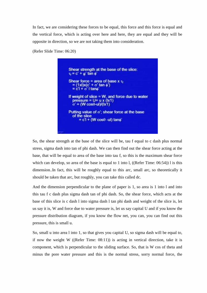
So, the shear strength at the base of the slice will be, tau f equal to c dash plus normal

stress, sigma dash into tan of phi dash. We can then find out the shear force acting at the

base, that will be equal to area of the base into tau f, so this is the maximum shear force

which can develop, so area of the base is equal to 1 into l, ((Refer Time: 06:54)) l is this

dimension..In fact, this will be roughly equal to this arc, small arc, so theoretically it

should be taken that arc, but roughly, you can take this called dc.

And the dimension perpendicular to the plane of paper is 1, so area is 1 into l and into

this tau f c dash plus sigma dash tan of phi dash. So, the shear force, which acts at the

base of this slice is c dash l into sigma dash l tan phi dash and weight of the slice is, let

us say it is, W and force due to water pressure is, let us say capital U and if you know the

pressure distribution diagram, if you know the flow net, you can, you can find out this

pressure, this is small u.

So, small u into area l into 1, so that gives you capital U, so sigma dash will be equal to,

if now the weight W ((Refer Time: 08:11)) is acting in vertical direction, take it is

component, which is perpendicular to the sliding surface. So, that is W cos of theta and

minus the pore water pressure and this is the normal stress, sorry normal force, the

component of the force, which is acting in normal to the failure plane divided by area,

that gives you sigma dash.

So, now, put this value here, in this equation, so putting the value of sigma dash, the

shear force at the base of the slice, will be equal to c dash l plus, here you will be getting

W cos theta minus u l into tan of phi dash. So, this is the another force which is acting on

the slice.


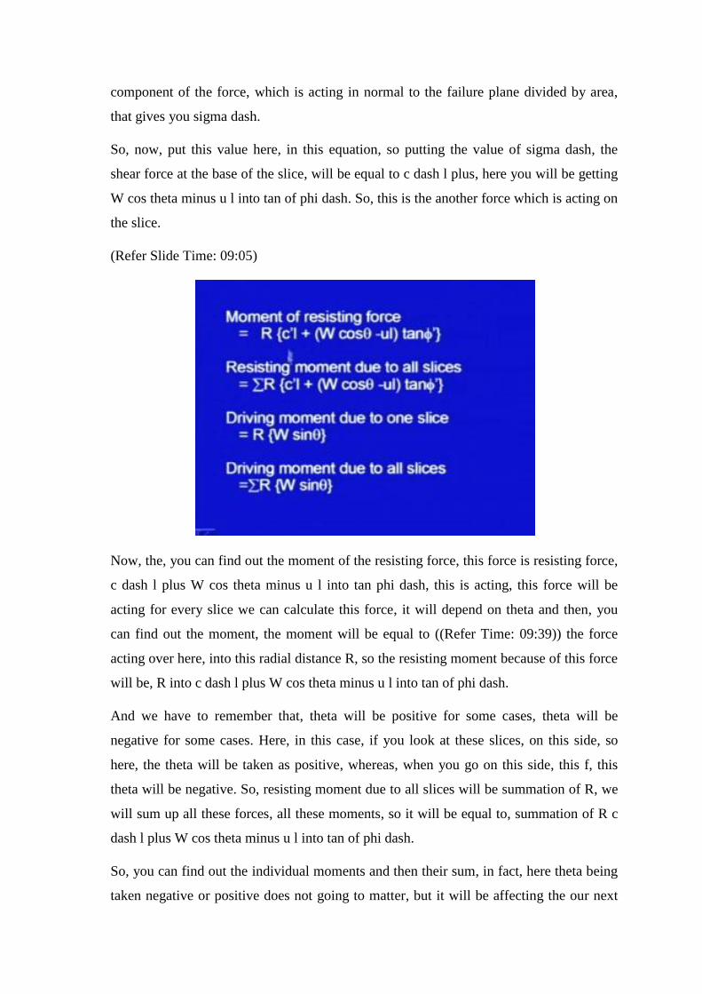
Now, the, you can find out the moment of the resisting force, this force is resisting force,

c dash l plus W cos theta minus u l into tan phi dash, this is acting, this force will be

acting for every slice we can calculate this force, it will depend on theta and then, you

can find out the moment, the moment will be equal to ((Refer Time: 09:39)) the force

acting over here, into this radial distance R, so the resisting moment because of this force

will be, R into c dash l plus W cos theta minus u l into tan of phi dash.

And we have to remember that, theta will be positive for some cases, theta will be

negative for some cases. Here, in this case, if you look at these slices, on this side, so

here, the theta will be taken as positive, whereas, when you go on this side, this f, this

theta will be negative. So, resisting moment due to all slices will be summation of R, we

will sum up all these forces, all these moments, so it will be equal to, summation of R c

dash l plus W cos theta minus u l into tan of phi dash.

So, you can find out the individual moments and then their sum, in fact, here theta being

taken negative or positive does not going to matter, but it will be affecting the our next

point, so here, the driving moment due to one slice, so this was the resisting moment.

Now, let us calculate the driving moment, the another component W sin theta, this is the

component of the weight, which is acting tangentially to the failure plane, so it is, the

moment will be equal to R into sin into theta.

So, here, it will matter, whether you take theta is equal to positive or negative, so for

example, if you take theta here, here it is trying to drive this, it is trying to fail, whereas,

on this side, theta is in this direction, it is trying to stabilize the slope. So, driving

moment due to one slice will be, R is the radius into component of the weight, which is

acting tangentially to the failure plane. So, now, driving moment due to all slices will be

equal to summation of R W sin theta.

So, we will find out W sin theta for each of the slice and then, multiplied by R, take their

sum, that gives you the total driving moment.


And as you know, the factor of safety will be equal to, total driving moment divided by

total, sorry total resisting moment divided by total driving moment. So, when we put it

here in this equation, R being constant, you can take it out from this term, from

numerator, as well as from denominator, so R will cancel and factor of safety, will be

given as summation of c dash l plus W cos theta minus u l tan phi dash upon summation

of W sin theta.

So, what we have to do is, for individual slices, we will be calculating W, we will be

calculating theta, we will be calculating u l and then, we will find out this numerical, this

numerator and also, we will find out denominator and then, by taking this ratio, we will

be able to find out factor of safety. This expression, is in terms of the effective stresses, if

you are working in terms of total stress analysis, then the same expression will be there

will, with little change, it will be, Fs will be equal to c total into l plus W cos theta tan of

phi t.

So, here, we in case of the effective stresses we have taken the pour water pressure

separately. So,(( Refer Time: 13:54)) there it will come in this term, so W cos theta tan

of phi t divided by summation of W sin theta.


Let us demonstrate the applicability of this method through one example, here it is given

that, there is a slope as shown in the figure. Take phi dash for all the three soils as 20

degree, unit weight in kilonewton per meter cube and c dash in kilopascal, are mentioned

in the figure, determine the factor of safety using ordinary method of slices.


So, here it is a slope given to us, so the slope given was, this was the top level and here,

this is the toe and it is not having uniform gradient uniform profile. So, here to here, the

gradient is different, here to here, gradient is flatter, so we have taken first trial circle, I

will be showing only for the first trial circle and then, we draw a circle and then, we have

join these points by straight lines also, so that, is not going to matter much, whether I, we

take the circular surface or the straight line, here.

And for any slice, for example, let us say slice number 7, this is the inclination of the

failure surface with horizontal, which I have denoted here, by angle theta. The soil is not

homogeneous, here it is 17, gamma is 17 kilonewton per meter cube, it is 18 here, 18.5

here, c dash is also different, so it is 40, 80 and 100 kpa. We have divided the slope into

slices, 1, 2, 3, 4, 5, 6, 7, 8, 9, it is as per our convenience and as discussed last time, for

the sake of making the computations simple.

I have taken one slice endings here, where the profile is ending, same way, one slice

should end here, you can have uniform width also and here also, I have taken, this at the

intersection I have taken one slice ending here and here, at the intersection of the failure

surface and where the profile is changing, so I have taken one slice. So that, the idea is

that, I can, the calculations will be simple, this entire material in one slice will be having

one property, this will be having one property.

Theoretically, you can take, as per your convenience any number of the slices and when

we take up the moments, you see that the distance lead ((Refer Time: 07:19)) the, I will

be shown here. This is the centre of the circle and you can see, these slices 4, 5, 6, 7, 8, 9,

these slices are trying to destabilize their forces, their component of the, if I take the

vertical weight and then, it is component parallel to the sliding surface, so the

components will be in this direction, here it will be in this direction, here it will be in this

direction and so on, up to you reach here, so here it will be almost horizontal.

Now, when you go to watch this, then the component tangential to the failure surface is

in this direction. So, they are trying to do opposite, so I have, we have taken d as positive

in this case and d is negative in this case.


So, the solution consist of, take a trial circle as shown in the figure, as I discussed, then

divide the mass into number of slices, as per our convenience. In case of homogeneous

soil mass, equal base width could be taken, you can take even now also equal base width

and you can do the computations, but, there will be little bit more computations. Then,

compute weight of each slice, means W, it is base length means length of the failure

surface for that slice and the inclination, theta at which that base is inclined with the

horizontal.

And also, if water table is present, then compute U, capital U is the force or total

pressure, it will be small u into l, small u you can find out from the flow net and then,

you can multiply it with the base length and you can get capital U.


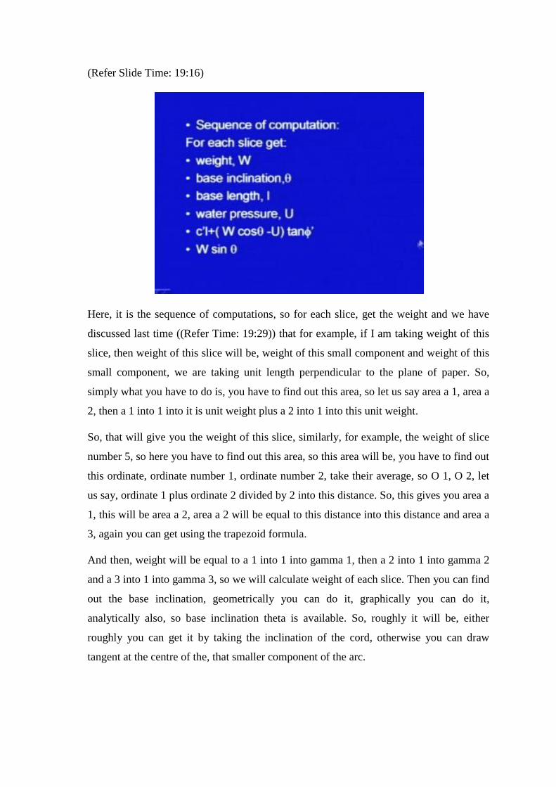
Here, it is the sequence of computations, so for each slice, get the weight and we have

discussed last time ((Refer Time: 19:29)) that for example, if I am taking weight of this

slice, then weight of this slice will be, weight of this small component and weight of this

small component, we are taking unit length perpendicular to the plane of paper. So,

simply what you have to do is, you have to find out this area, so let us say area a 1, area a

2, then a 1 into 1 into it is unit weight plus a 2 into 1 into this unit weight.

So, that will give you the weight of this slice, similarly, for example, the weight of slice

number 5, so here you have to find out this area, so this area will be, you have to find out

this ordinate, ordinate number 1, ordinate number 2, take their average, so O 1, O 2, let

us say, ordinate 1 plus ordinate 2 divided by 2 into this distance. So, this gives you area a

1, this will be area a 2, area a 2 will be equal to this distance into this distance and area a

3, again you can get using the trapezoid formula.

And then, weight will be equal to a 1 into 1 into gamma 1, then a 2 into 1 into gamma 2

and a 3 into 1 into gamma 3, so we will calculate weight of each slice. Then you can find

out the base inclination, geometrically you can do it, graphically you can do it,

analytically also, so base inclination theta is available. So, roughly it will be, either

roughly you can get it by taking the inclination of the cord, otherwise you can draw

tangent at the centre of the, that smaller component of the arc.

So, base inclination theta you can find out, then base length, either circular or cord, you

can take the cord length, then water pressure, is equal to U into l. Then, compute this c

dash l plus W cos theta minus U tan phi dash and compute W sin theta for each of them.


Here, I have shown the computations, this is slice number 1, weight is 714 newton, sorry

kilonewton, then it is base length is 1.5 meter, theta is, here theta, I have taken negative,

this is slice number 1, so theta is negative here. This is the base length, this is c dash, this

is phi dash, this is the numerical, this is the numerator c dash l plus W minus U into this

value ((Refer Time: 22:29)), this value, it is in that column and W sin theta is in this

column.

In this table, this is the base length and in fact, this is the base width of the slice, so you

can calculate all these values, finally what we need is summation of these terms,

summation of c dash l plus, so c dash l plus W cos theta minus U into tan phi dash. These

are these values, in this column and these are W sin theta values, for individual slices and

their sum is 13003 and 5171.


Finally, the factor of safety is, this is the term in the numerator, which we had calculated,

so summation of c dash l plus W cos theta minus u l tan phi dash, it comes out to be

equal to this much, summation of W sin theta is 5171 and factor of safety, then we get

2.51. So, this is the factor of safety for the trial circle, which we have taken in this case

and to get the factor of safety of the slope.

Further trials are required with another circles and we have to take large number of

circles, we have to calculate factor of safety for all of them and minimum has to be

selected, as the factor of safety of the slope and that circle will be the critical circle.


Now, let me discuss the same method, ordinary method of slices, but to solve the

problem graphically, earlier we discussed the analytical method, using which you can

write a computer program. So, graphical method can also be used, basic steps are same,

we assume a trial failure surface, then divide the mass above the failure surface in slices

of equal width, let us say 8 or 10, so it is not necessary you can have unequal widths

also, then consider the force acting on each slice.


So, here, this is the graphical method and we have taken all the slices having same width,

so this is the trial circle, center is O, radius is R and if you take any slice, let us say Nth

slide here, slice, height is h, weight is acting in downward direction, so here it is the

weight, this is the weight of the slice, slice number let us say, 1, 2, 3, this is the third

slice. So, weight is acting in this direction and it is two components, one component will

be normal to the failure surface.

So, this is the normal, normal means it is the radial vector, so straight way you can have

a straight line joining from point O and midpoint of this slice. So, take midpoint of this

slice, draw vertical line here, at mid of this slice and then, join this point on the periphery

and centre and extend it. So, this will have to automatically be, normal to the tangential

surface, sorry the failure surface and a, b, this denotes the weight graphically, so you can

draw it graphically this much.

And from here, from we, draw a line parallel to the tangent here or you can say, normal

to the radial vector, so this angle will be 90, draw a line at 90 degree and get the

intersection point C, so you will be getting N 3, T 3 and this angle will be, let us say

theta. So, you can get N component, you can get T component, same thing is here, join it

with the centre, extend it, but the direction of T now, in this case is opposite. So, you

have to and this W 7 represents the weight of this slice.


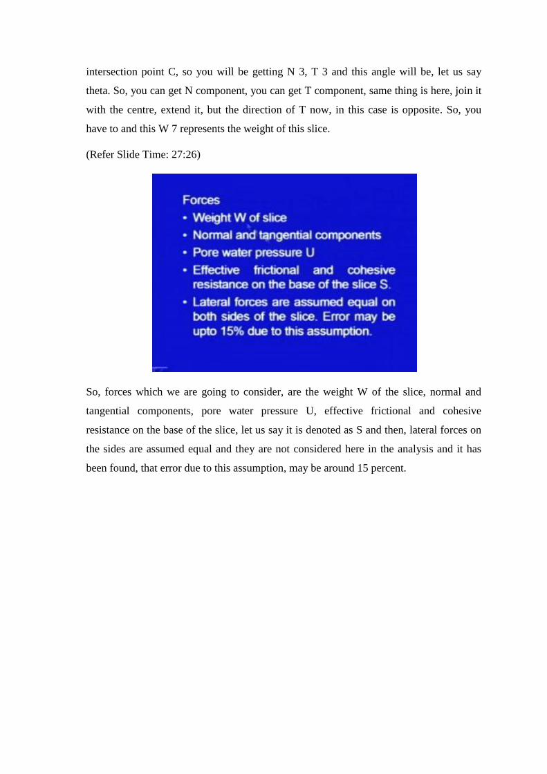
So, forces which we are going to consider, are the weight W of the slice, normal and

tangential components, pore water pressure U, effective frictional and cohesive

resistance on the base of the slice, let us say it is denoted as S and then, lateral forces on

the sides are assumed equal and they are not considered here in the analysis and it has

been found, that error due to this assumption, may be around 15 percent.


This is the pore wet water pressure diagram, so here, it is the circle which is, trial circle

which we have drawn and then you can draw the pore water pressure diagram, the pore

water pressure acting at different points at the centers of the slices, this is for example, U

and l 1, this is U 2 l 2, l is in fact, this distance and then, you can find out, you can draw

this pore water pressure diagram, using which, we will be getting the pore water

pressures.


Now, graphically, to calculate the different forces, let us start with the weight W, so this

is the third slice, which we are taking into consideration, weight will be equal to gamma

into h into b into, h is the average height of the slice, b is width of the slice, so h into b

gives you area, we can, we are considering this arc as a straight line, approximately a

straight line. So, h into b and perpendicular, sorry normal to the plane of paper we are

taking one unit dimension, so volume of this slice will be h into b into 1 and gamma is

the unit weight of soil, so gamma h b is the unit weight.

Now, if we keep the widths of all the slices same and also, if the mass is homogeneous,

then W can be plotted as a vector A B, we can see, here in this case we can directly then

take W as A, W can be calculated as a function of h only, because we are taking b

constant, width is constant, gamma is constant, because it is homogeneous, so gamma

into b will become constant for each slice and only you have to multiply, small h. So,

straight way, we can draw this W 3, straightway h times that constant value, that is

gamma into b.

So, W is plotted here and then A B can be made equal to the height of the slice, as far as

graphical construction is concerned, see we can graphically, simply plot, this W equal to

h only and when we do the calculations, we will multiply it by gamma into b, But

remember, in that case, this should be homogeneous, soil should be homogeneous and

width should be same, for all the slices.

So, we can draw here, h length we can draw and as I told you, you can draw radial vector

and draw here, a line perpendicular to radial vector, then you can get the component N

and component T.


Construct the triangle A B C, construct this triangle and resolve the components and get

N and T, the component T causes the instability. So, this is what we have been

discussing, this component T, which is acting over here, this is causing instability and

this component N, it is going to give the normal stress, will from which, using which the

slice, which will derive it is resistance, shearing resistance.

So, we can now plot the, it is very convenient on a graph paper, you can just plot another

h here, plot radial vector plot, another h here, plot radial vector and so on. Then you can

get the sum of the all components summation of T.


And, if the trial surface is curved upward near it is lower end, T will act in opposite

direction, this point also I have discussed earlier, so here, near the toe, if the, if the slope

is, be the failure surface is dipping in this direction, so T will be in opposite direction, so

it will be negative in this case.


So, get average pressure u acting on the base of any slice, the total pore pressure on the

base of the slice will be u into, u will be, capital U will be equal to small u into l. Then,

effective normal pressure N dash acting on the base of the slice will be equal to N minus

U, the frictional force F dash acting on the base of any slice will be equal to, F equal to N

minus U tan of phi dash.


And also, the cohesive force C dash, opposing the movement of the slice and acting at

the base of the slice will be c dash into l.


So, we will talk in terms of these forces, so this is the slice, it is weight is there and we

have got the N component and T components. So, this is the base of the slice and here it

is the N component and you have got the water pressure, so you, so we subtract it, so out

of N, only N minus U is left. So, what we have to do, to get the frictional component,

make draw a line at phi dash angle, so when you draw it, so this much into tan of phi

dash is this, so this component F dash, this is N minus U tan of phi dash.

So, graphically you can obtain, you can get this ordinate and also, this is the cohesive

component, c dash into l, so c dash into l and plus this, this will be the shear total

resisting force S at the base of the slice. So, this you can do, for the each of the slice, this

component can be obtained.


Now, when you take sum of all the resisting forces, so S will be, S s will be, c dash

summation of l plus tan phi dash, summation of N minus U, C dash is the constant term

and tan phi dash is also constant, here we had assumed that this soil is homogeneous.

The moment of actuating forces will be R into summation T, we have already discussed

T is the actuating component. So, it is moment will be R into summation of T and the

resisting moment will be R into c dash L plus tan phi summation of N minus U.

Here, I have replaced this summation of l by capital L here, capital L is the total length

of the circular arc, so summation of small l will be nothing but capital L. So, the moment

of the resisting forces will be R into this much and moment of actuating force is this

much, R into summation of T, so the factor of safety will be, ratio of this to this, so F s is

equal to c dash into capital L plus tan phi dash into summation of N minus U upon

summation of T.

So, for each slice we are going to get this, tan phi dash into N minus U and then, we can

get the factor of safety.


Here, it is the graphical representation of the factor of safety, to get the factor of safety

graphically, now what we do is, plot this A B, equal to summation of N minus U, you are

getting N minus U for each of the slice. So, from there, you can get total sum, so this is,

A B is representing summation of N minus U and then draw perpendicular line here and

draw a line A D, which is inclined at an angle phi dash, so this D B will become equal to

tan of phi dash into summation of N minus U, so, this much, so D B, BD is equal to that

much.

So, this is the frictional component and then, add here extend it, up to C and D C is equal

to frictional, cohesive component c dash into capital L. So, B into C, that becomes total

numerator of the factor of safety expression and then, divided by B E, so this is another

point which we have drawn, this is taken as equal to summation of T. T also you got for

different slices, so summation of T you can get, draw B E equal to summation of T and

then, factor of safety will be equal to B C upon B E, B C divided by B E, this gives you

the factor of the safety.


Now, again, large number of trial circles are required to be taken, then out of those, then

we will select the minimum factor of safety and that is going to give you critical circle

and the factor of safety. Now here, you have seen that, not only in this graphical method,

but also in analytical method, we have to take large number of trials. So, here is a

procedure, an approximate procedure, which can reduce those large number of trials, to

avoid the large number of trials, the following method is adopted.

Get direction angles alpha A and alpha B, from the table and get point A by drawing

these angles as shown in the figure.


So, first of all, let us say, this is the slope angle 60, 45 and so on, these are the slope in

terms of the ratios and this is a table, suggested table, so you have to get corresponding

to that slope. For example, let us say beta is equal to 45 degree, then direction angle,

alpha A is 28, alpha B is 37, suppose, it is 30 degree, then you have to interpolate

between this and this, so alpha A between this and this, alpha B, then you can take here.

So, using these values then you have to draw this figure.


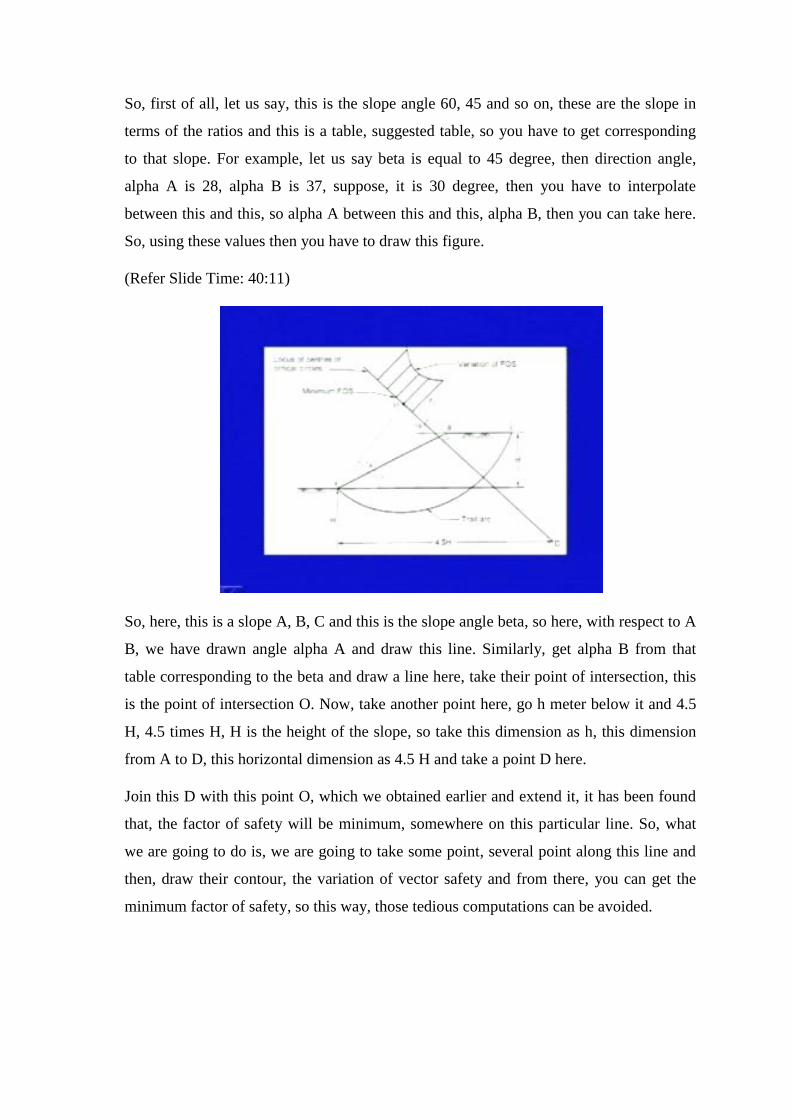
So, here, this is a slope A, B, C and this is the slope angle beta, so here, with respect to A

B, we have drawn angle alpha A and draw this line. Similarly, get alpha B from that

table corresponding to the beta and draw a line here, take their point of intersection, this

is the point of intersection O. Now, take another point here, go h meter below it and 4.5

H, 4.5 times H, H is the height of the slope, so take this dimension as h, this dimension

from A to D, this horizontal dimension as 4.5 H and take a point D here.

Join this D with this point O, which we obtained earlier and extend it, it has been found

that, the factor of safety will be minimum, somewhere on this particular line. So, what

we are going to do is, we are going to take some point, several point along this line and

then, draw their contour, the variation of vector safety and from there, you can get the

minimum factor of safety, so this way, those tedious computations can be avoided.


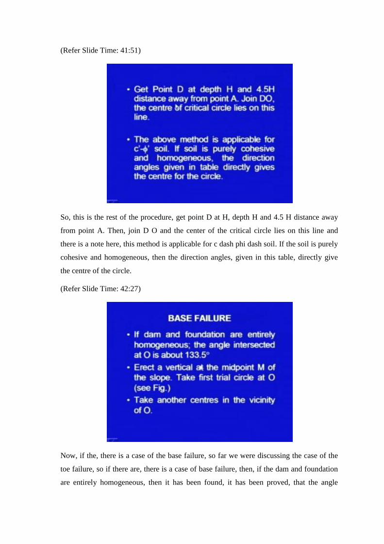
So, this is the rest of the procedure, get point D at H, depth H and 4.5 H distance away

from point A. Then, join D O and the center of the critical circle lies on this line and

there is a note here, this method is applicable for c dash phi dash soil. If the soil is purely

cohesive and homogeneous, then the direction angles, given in this table, directly give

the centre of the circle.


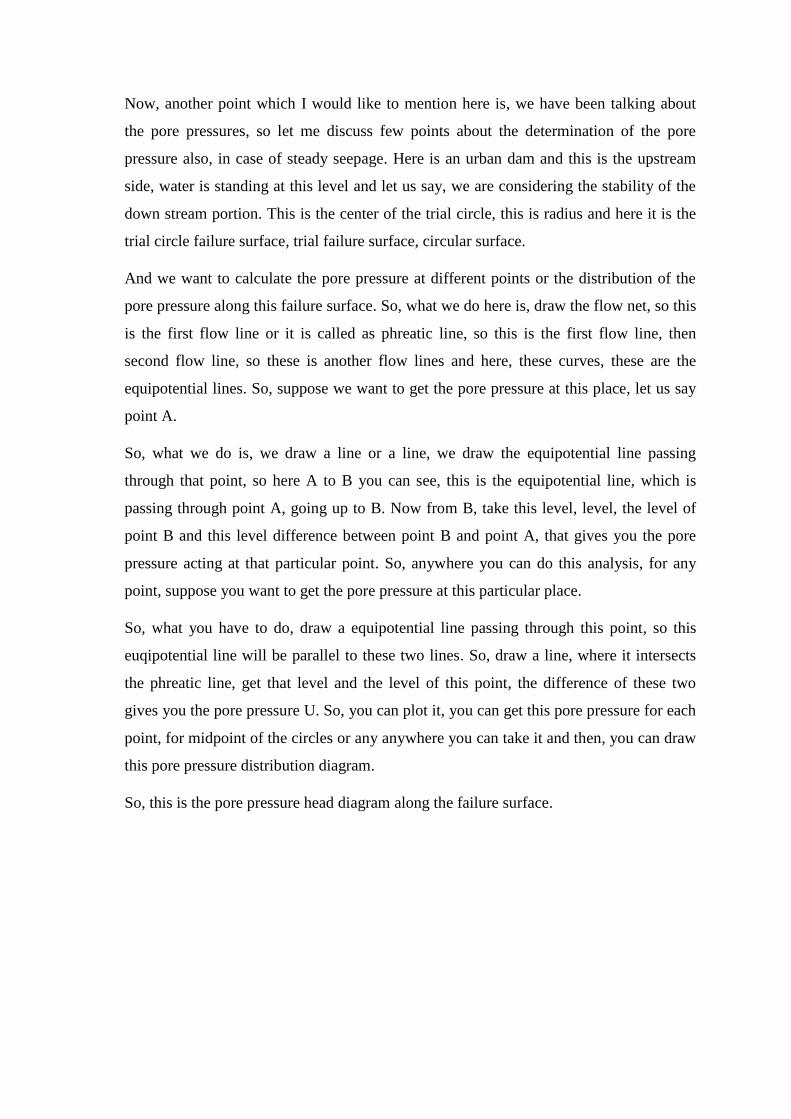
Now, if the, there is a case of the base failure, so far we were discussing the case of the

toe failure, so if there are, there is a case of base failure, then, if the dam and foundation

are entirely homogeneous, then it has been found, it has been proved, that the angle

intersected at the center is about 133.5 degree. So, we use this information, as well as the

information that the center of the critical circle should be above the midpoint, so erect a

vertical at the midpoint M of the slope.


So, here, this is the slope, so what we have done here is, this is the point M, so the

critical circle will be on this line, it is known and then, this angle is 133.5, so this is the

information ((Refer Time: 43:30)) which is quite useful. So, we erect a vertical, take the

trial circle at this, as shown here, so take this 133.5 degree angle and then, take the next

trials, so using this information also, one can reduce the computations.


Now, another point which I would like to mention here is, we have been talking about

the pore pressures, so let me discuss few points about the determination of the pore

pressure also, in case of steady seepage. Here is an urban dam and this is the upstream

side, water is standing at this level and let us say, we are considering the stability of the

down stream portion. This is the center of the trial circle, this is radius and here it is the

trial circle failure surface, trial failure surface, circular surface.

And we want to calculate the pore pressure at different points or the distribution of the

pore pressure along this failure surface. So, what we do here is, draw the flow net, so this

is the first flow line or it is called as phreatic line, so this is the first flow line, then

second flow line, so these is another flow lines and here, these curves, these are the

equipotential lines. So, suppose we want to get the pore pressure at this place, let us say

point A.

So, what we do is, we draw a line or a line, we draw the equipotential line passing

through that point, so here A to B you can see, this is the equipotential line, which is

passing through point A, going up to B. Now from B, take this level, level, the level of

point B and this level difference between point B and point A, that gives you the pore

pressure acting at that particular point. So, anywhere you can do this analysis, for any

point, suppose you want to get the pore pressure at this particular place.

So, what you have to do, draw a equipotential line passing through this point, so this

euqipotential line will be parallel to these two lines. So, draw a line, where it intersects

the phreatic line, get that level and the level of this point, the difference of these two

gives you the pore pressure U. So, you can plot it, you can get this pore pressure for each

point, for midpoint of the circles or any anywhere you can take it and then, you can draw

this pore pressure distribution diagram.

So, this is the pore pressure head diagram along the failure surface.


So, here it is the method, draw the flow net, then to get pressure head at any point a,

draw equipotential line passing through the point a. Get point b, which is the intersection

of equipotential line with the phreatic line and then, elevation difference between a and b

gives the pressure head at point a.


Now, let us come to the most popular method, the Bishop’s simplified method of slices.


Here, it is the, these are the basic concept, again the same slope I have taken a slope,

with some angle here and this is the center of the circle, this is a trial circle which we

have taken and then, we have divided the slices into, sorry the mass into some number of

slices and this is, let us say this slice under consideration. This is the point, joining the

point O, with the midpoint here at the sliding surface, inclination of the base is theta

degree and this slice is shown here.

Now, you can see, in this case now, we are taking the side forces also, so W is acting, the

weight of the slice is acting in downward direction and the, on the right hand side, the

side force along the surface is acting in downward direction. On the left hands vertical

face, this force will be acting in upward direction, let us say, it is T 2 here and T 1 here.

There is a horizontal force even on the right hand side face and on the left hand side face,

the force E 2 is there.

N is the normal force, which is acting normal to the failure surface, N dash, it is the N

dash force and here, it is U, U is the pore water pressure, length of this base is l and as a

whole when you do the analysis, you can it is, the force T 2, you see, it is acting on in

upward direction for this slice. So, T 2, here it is acting in upward direction for this slice,

when we consider the next slice, this one, so the same T 2 will be acting in downward

direction.

So, and similarly here, there will be another force, which will be acting on this slice in

upward direction and on adjoining slice, it will be acting in downward direction. So, as a

whole, when you sum up these forces, these T forces and E forces for the entire mass,

when you sum them up, they should be equal to 0.


.

Now, the forces which we are considering here are, we W is the weight of the slice, N is

the total normal force on the failure surface dc. At the base, U is pore water pressure

equal to u into l, N was the total normal force and N dash will be equal, to the effective

normal force and F R is the shear resistance on the surface d c. Here, ((Refer Time:

51:10)) this is the base and F R is the shear resistance, E 1, E 2 are the normal forces on

the vertical faces of the slice and they will be opposite to each other.

And T 1 and T 2, they will also be opposite to each other, they are shear forces on

vertical faces, so here, T 1, T 2 opposite direction and E 1, E 2.


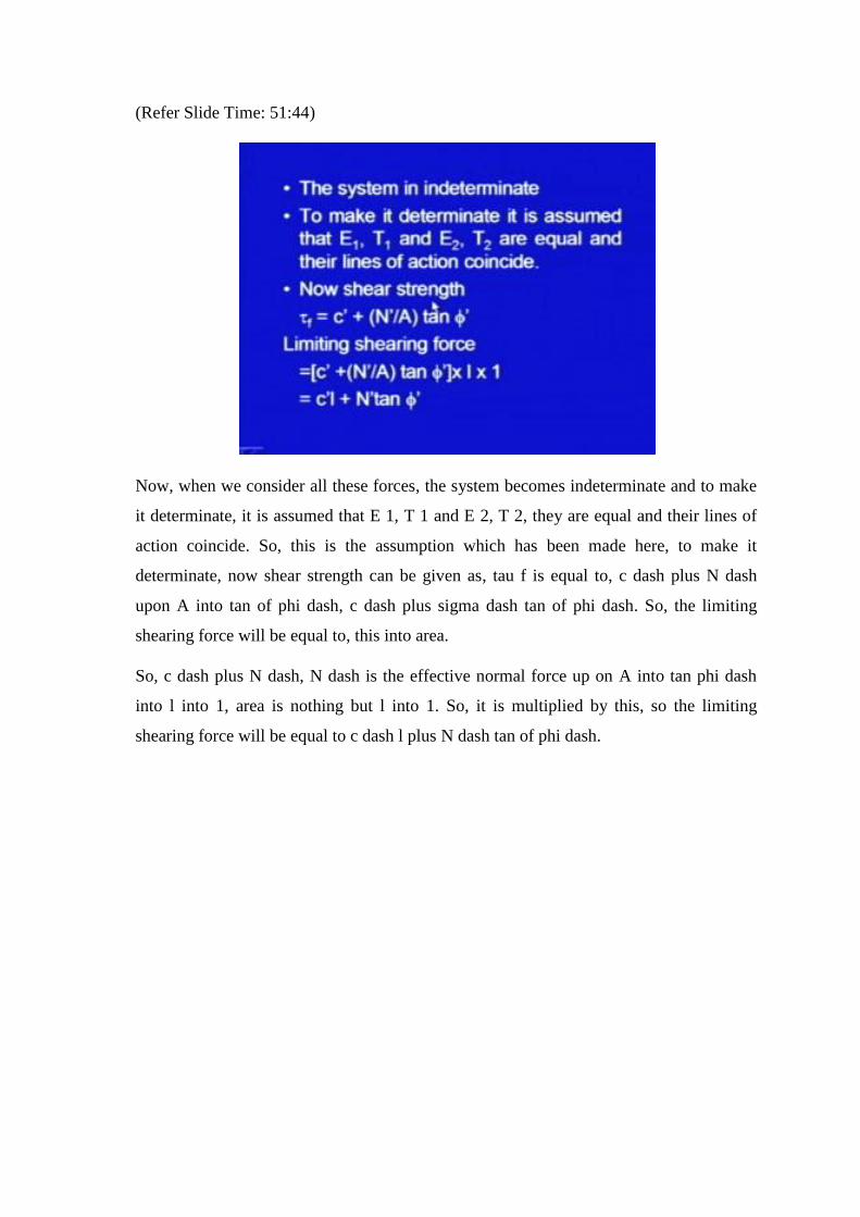
Now, when we consider all these forces, the system becomes indeterminate and to make

it determinate, it is assumed that E 1, T 1 and E 2, T 2, they are equal and their lines of

action coincide. So, this is the assumption which has been made here, to make it

determinate, now shear strength can be given as, tau f is equal to, c dash plus N dash

upon A into tan of phi dash, c dash plus sigma dash tan of phi dash. So, the limiting

shearing force will be equal to, this into area.

So, c dash plus N dash, N dash is the effective normal force up on A into tan phi dash

into l into 1, area is nothing but l into 1. So, it is multiplied by this, so the limiting

shearing force will be equal to c dash l plus N dash tan of phi dash.


And if the factor of safety is F s, then the mobilized shearing resistance at the base of the

slice will be equal to, F R will be equal to c dash l upon F s plus N dash tan of phi dash

upon F s.


Now here, I consider the equilibrium of the vertical forces, so W is acting in downward

direction and T 1, T 2 presently we are taking in into account for general solution, but for

simplified cases, then we will take it to be equal to 0. So, T 1 is acting here, so let us take

a general case, T 1 is there, T 2 is there, E 1 is also there, E 2 is also there and we are

considering the equilibrium of vertical forces, so the horizontal forces will not come into

picture.

So, W plus T 1 minus T 2 and minus this U is acting here, so U cos theta and then

component of F R will also, so vertical component of F R will be F R sin theta and

vertical component of N dash will be N dash cos theta. So, this equation will be there and

total sum should be equal to 0, because we are considering the slice to be in equilibrium.

Now, putting the value of F R which we just now calculated,((Refer Time: 54:47))we

computed previously using this value, when we put F R here and solve this equation.


We get following expression for N dash, so N dash is equal to, W plus delta T, delta T is

T 1 minus T 2 minus U cos theta divided by c dash l upon F s sin theta upon cos theta

plus tan phi dash sin theta upon F s and now here, we will put it again back into the

expression of F R. So, F R is equal to c dash l upon F s plus N dash tan phi dash upon F

s, so we get F R is equal to c dash l upon F s and put this N dash here. So, this becomes,

W minus U cos theta plus delta T minus c dash l upon F s sin theta divided by cos theta

plus tan phi dash sin theta upon F s into tan phi dash upon F s.

So, let me stop here itself and on the next time I will be completing this, today we have

discussed about the method of slices and we have started discussing about the Bishop’s

method and this Bishop’s simplified method is probably the most widely used method

and I have come up to half of the derivation of this method and rest of the things, we will

be doing in the next class.

Thank you.

Date post:	08-Sep-2018
Category:	Documents
Upload:	truongdang
View:	225 times
Download:	0 times

Foundation Engineering Prof. Mahendra Singh …textofvideo.nptel.ac.in/105107120/lec39.pdf ·...

Documents