5-1 THE SETTLEMENT PROBLEM Foundation settlements must be estimated with great care for buildings, bridges, towers, power plants, and similar high-cost structures. For structures such as fills, earth dams, levees, braced sheeting, and retaining walls a greater margin of error in the settlements can usually be tolerated. Except for occasional happy coincidences, soil settlement computations are only best es- timates of the deformation to expect when a load is applied. During settlement the soil tran- sitions from the current body (or self-weight) stress state to a new one under the additional applied load. The stress change Aq from this added load produces a time-dependent accu- mulation of particle rolling, sliding, crushing, and elastic distortions in a limited influence zone beneath the loaded area. The statistical accumulation of movements in the direction of interest is the settlement. In the vertical direction the settlement will be defined as AH. The principal components of AH are particle rolling and sliding, which produce a change in the void ratio, and grain crushing, which alters the material slightly. Only a very small frac- tion of A// is due to elastic deformation of the soil grains. As a consequence, if the applied stress is removed, very little of the settlement AH is recovered. Even though AH has only a very small elastic component, it is convenient to treat the soil as a pseudo-elastic material with "elastic" parameters E 59 G', /i,, and k s to estimate settlements. This would appear reason- able because a stress change causes the settlement, and larger stress changes produce larger settlements. Also experience indicates that this methodology provides satisfactory solutions. There are two major problems with soil settlement analyses: 1. Obtaining reliable values of the "elastic" parameters. Problems of recovering "undis- turbed" soil samples mean that laboratory values are often in error by 50 percent or more. There is now a greater tendency to use in situ tests, but a major drawback is they tend to obtain horizontal values. Anisotropy is a common occurrence, making vertical elastic FOUNDATION SETTLEMENTS CHAPTER 5
Transcript
5-1 THE SETTLEMENT PROBLEM
Foundation settlements must be estimated with great care for buildings, bridges, towers,power plants, and similar high-cost structures. For structures such as fills, earth dams, levees,braced sheeting, and retaining walls a greater margin of error in the settlements can usuallybe tolerated.
Except for occasional happy coincidences, soil settlement computations are only best es-timates of the deformation to expect when a load is applied. During settlement the soil tran-sitions from the current body (or self-weight) stress state to a new one under the additionalapplied load. The stress change Aq from this added load produces a time-dependent accu-mulation of particle rolling, sliding, crushing, and elastic distortions in a limited influencezone beneath the loaded area. The statistical accumulation of movements in the direction ofinterest is the settlement. In the vertical direction the settlement will be defined as AH.
The principal components of AH are particle rolling and sliding, which produce a changein the void ratio, and grain crushing, which alters the material slightly. Only a very small frac-tion of A// is due to elastic deformation of the soil grains. As a consequence, if the appliedstress is removed, very little of the settlement AH is recovered. Even though AH has onlya very small elastic component, it is convenient to treat the soil as a pseudo-elastic materialwith "elastic" parameters E59 G', /i,, and ks to estimate settlements. This would appear reason-able because a stress change causes the settlement, and larger stress changes produce largersettlements. Also experience indicates that this methodology provides satisfactory solutions.
There are two major problems with soil settlement analyses:
1. Obtaining reliable values of the "elastic" parameters. Problems of recovering "undis-turbed" soil samples mean that laboratory values are often in error by 50 percent or more.There is now a greater tendency to use in situ tests, but a major drawback is they tendto obtain horizontal values. Anisotropy is a common occurrence, making vertical elastic
FOUNDATION SETTLEMENTS
CHAPTER
5
values (usually needed) different from horizontal ones. Often the difference is substantial.Because of these problems, correlations are commonly used, particularly for preliminarydesign studies. More than one set of elastic parameters must be obtained (or estimated) ifthere is stratification in the zone of influence H.
2. Obtaining a reliable stress profile from the applied load. We have the problem of com-puting both the correct numerical values and the effective depth H of the influence zone.Theory of Elasticity equations are usually used for the stress computations, with the in-fluence depth H below the loaded area taken from H = 0 to H -» o° (but more correctlyfrom 0 to about AB or 5B). Since the Theory of Elasticity usually assumes an isotropic,homogeneous soil, agreement between computations and reality is often a happy coinci-dence.
The values from these two problem areas are then used in an equation of the general form
AH = \ edHJo
where e = strain = Aq/Es\ but Aq = f(H, load), Es = f(H, soil variation), and H (as pre-viously noted) is the estimated depth of stress change caused by the foundation load. Theprincipal focus in this chapter will be on obtaining Aq, Es and H.
It is not uncommon for the ratio of measured to computed AH to range as 0.5 <— ^mea* —>2. Current methodology tends to minimize "estimation" somewhat so that most ratios are inthe 0.8 to 1.2 range. Note too that a small computed AH of, say, 10 mm, where the measuredvalue is 5 or 20 mm, has a large "error," but most practical structures can tolerate either thepredicted or measured value. What we do not want is an estimate of 25 mm and a subsequentsettlement of 100 mm. If we err in settlement computations it is preferable to have computedvalues larger than the actual (or measured) ones—but we must be careful that the "large"value is not so conservative that expensive (but unneeded) remedial action is required.
Settlements are usually classified as follows:
1. Immediate, or those that take place as the load is applied or within a time period of about7 days.
2. Consolidation, or those that are time-dependent and take months to years to develop. TheLeaning Tower of Pisa in Italy has been undergoing consolidation settlement for over 700years. The lean is caused by the consolidation settlement being greater on one side. This,however, is an extreme case with the principal settlements for most projects occurring in3 to 10 years.
Immediate settlement analyses are used for all fine-grained soils including silts and clayswith a degree of saturation S ^ 90 percent and for all coarse-grained soils with a large coef-ficient of permeability [say, above 10~3 m/s (see Table 2-3)].
Consolidation settlement analyses are used for all saturated, or nearly saturated, fine-grained soils where the consolidation theory of Sec. 2-10 applies. For these soils we wantestimates of both settlement AH and how long a time it will take for most of the settlementto occur.
Both types of settlement analyses are in the form of
AH = eH = V - ^ (i = 1 to n) (5-1)
where the reader may note that the left part of this equation is also Eq. (2-43<z). In practicethe summation form shown on the right may be used where the soil is subdivided into layersof thickness Ht and stresses and properties of that layer used. The total settlement is the sumobtained from all n layers. The reader should also note that Es used in this equation is theconstrained modulus defined from a consolidation test as \/mv or from a triaxial test usingEq. (e) of Sec. 2-14, written as
ts~ mv~ (1 + M ) (1 -2 /1 ) {5la)
where ESyir = triaxial value [also used in Eq. (5-16)]. Note, however, that if the triaxial cellconfining pressure 0-3 approximates that developed in situ when the load is applied, the tri-axial Es will approximate l/mv. In most cases the actual settlements will be somewhere be-tween settlements computed using the equivalent of \/mv as from a consolidation test [see Eq.(5- Ia)] and Es from a triaxial test. Unfortunately the use of Eq. (5- Ia) also requires estimatinga value of Poisson's ratio /JL.
5-2 STRESSES IN SOIL MASS DUETO FOOTING PRESSURE
As we see from Eq. (5-1), we need an estimate of the pressure increase Ag from the appliedload. Several methods can be used to estimate the increased pressure at some depth in thestrata below the loaded area. An early method (not much used at present) is to use a 2 : 1slope as shown in Fig. 5-1. This had a great advantage of simplicity. Others have proposedthe slope angle be anywhere from 30° to 45°. If the stress zone is defined by a 2 : 1 slope, the
Figure 5-1 Approximate methods of obtaining the stress increase qv in the soil at a depth z beneath the footing.
pressure increase qv = Ag at a depth z beneath the loaded area due to base load1 Q is
A * - * - (B + ZXL+ Z) <5-2)
which simplifies for a square base (B X B) to
* = ( B T ^ (5-2a)
where terms are identified on Fig. 5-1. This 2 : 1 method compares reasonably well with moretheoretical methods [see Eq. (5-4)] from z\ = Bio about zi = 4B but should not be used inthe depth zone from z = 0 to B. The average stress increase in a stratum (H = Zi ~ Z\) is
fZ2 O 1 I O \Zl
4*»-I,<BT3S*-*-i?l-sH ^*5-3 THE BOUSSINESQ METHOD FOR qv
One of the most common methods for obtaining qv is the Boussinesq (ca. 1885) equation basedon the Theory of Elasticity. Boussinesq's equation considers a point load on the surface of asemi-infinite, homogeneous, isotropic, weightless, elastic half-space to obtain
qv = 2 ^ 2 c o s 5 0 (5-3)
where symbols are identified on Fig. 5-2a. From this figure we can also write tan0 = r/z,define a new term R2 = r2 + z2, and take cos5 6 — (z/R)5. With these terms inserted in Eq.
Figure 5-2 (a) Intensity of pressure q based on Boussinesq approach; (b) pressure at point of depth z below thecenter of the circular area acted on by intensity of pressure qo.
lrThe vertical base load uses P, V, and Q in this textbook and in the published literature; similarly, stress increasesfrom the base load are qv, Aqv, p, and A/?.
(5-3) we obtain
* = 3S (5-4)which is commonly written as
qv = ^ IAl + (r/z)2]5/2 = I A, (5-5)
Since the A^ term is a function only of the r/z ratio we may tabulate several values as follows:
////These values may be used to compute the vertical stress in the stratum as in the followingtwo examples.
Example 5-1. What is the vertical stress beneath a point load Q = 225 kN at depths of z = Om,0.6 m, 1.2 m, and 3.0 m?
Solution. We may write qv = (Q/z2)Ab = OAllQ/z2 (directly beneath Q we have r/z = 0). Sub-stituting z-values, we obtain the following:
z, m qv = 0.477(225)/z2, in kPa
0 oo
0.6 298 kPa1.2 • 74.53.0 11.9
Example 5-2. What is the vertical stress qv at point A of Fig. E5-2 for the two surface loads Q\and Q2I
Figure E5-2
Chart Methods
The purpose of foundations is to spread loads so that "point" loads with the accompanyingvery high stresses at the contact point (z = 0 of Example 5-1) are avoided. Thus, directuse of the Boussinesq equation is somewhat impractical until z is at a greater depth wherecomputations indicate the point and spread load stress effects converge. We can avoid this byconsidering the contact pressure qo to be applied to a circular area as shown in Fig. 5-2Z? sothe load Q can be written as
(A
Q= qodAJo
The stress on the soil element from the contact pressure qo on the surface area dA of Fig.5-2b is
but dA = 2rrrdr, and Eq. (a) becomes
C f Q 1
* = J0 d?[l+(r/OT*2™* r (b)
Performing the integration and inserting limits, we have
•-'•{"'-[i + oW-} <5-6)This equation can be used to obtain the stress qv directly at depth z for a round footing of radiusY (now r/z is a depth ratio measured along the base center). If we rearrange this equation, solvefor r/z, and take the positive root,
The interpretation of Eq. (c) is that the r/z ratio is also the relative size of a circular bearingarea such that, when loaded, it gives a unique pressure ratio qjqo on the soil element at adepth z in the stratum. If values of the qv/qo ratio are put into the equation, corresponding
Stnliitirtn
sum of stresses from the two loads
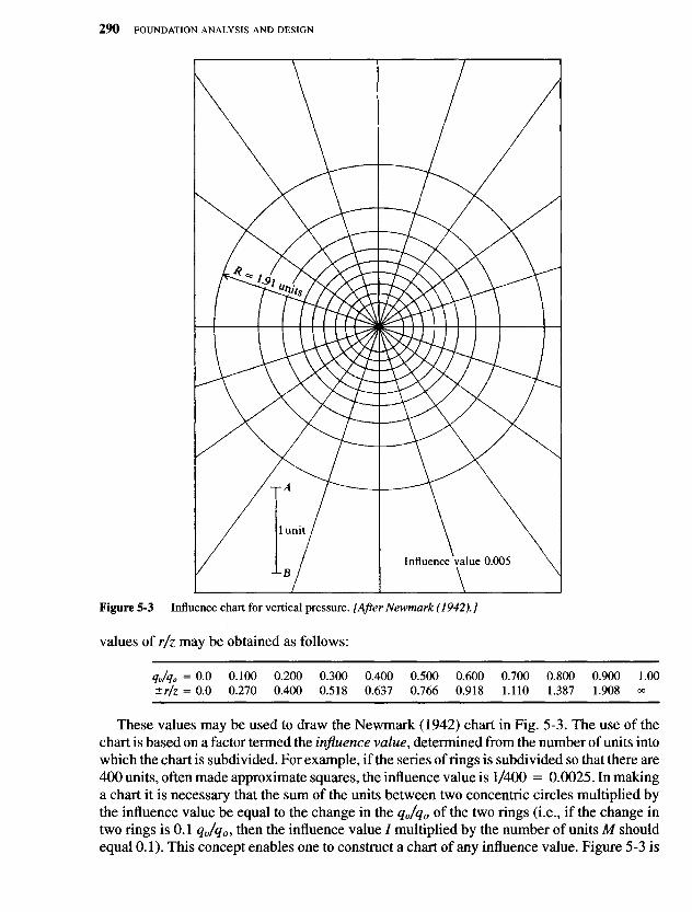
Figure 5-3 Influence chart for vertical pressure. [After Newmark (1942).]
These values may be used to draw the Newmark (1942) chart in Fig. 5-3. The use of thechart is based on a factor termed the influence value, determined from the number of units intowhich the chart is subdivided. For example, if the series of rings is subdivided so that there are400 units, often made approximate squares, the influence value is 1/400 = 0.0025. In makinga chart it is necessary that the sum of the units between two concentric circles multiplied bythe influence value be equal to the change in the qjqo of the two rings (i.e., if the change intwo rings is 0.1 qvlq0, then the influence value / multiplied by the number of units M shouldequal 0.1). This concept enables one to construct a chart of any influence value. Figure 5-3 is
Influence value 0.005
lunit
subdivided into 200 units; therefore, the influence value is 1/200 = 0.005. Smaller influencevalues increase the number of squares and the amount of work involved, since the sum ofthe squares used in a problem is merely a mechanical integration of Eq. (a). It is doubtful ifmuch accuracy is gained using very small influence values, although the amount of work isincreased considerably.
The influence chart may be used to compute the pressure on an element of soil beneath afooting, or from pattern of footings, and for any depth z below the footing. It is only necessaryto draw the footing pattern to a scale of z = length AB of the chart. Thus, if z = 5 m, thelength AB becomes 5 m; if z = 6 m, the length AB becomes 6 m; etc. Now if AB is 20mm, scales of 1 : 250 and 1 : 300, respectively, will be used to draw the footing plans. Thesefooting plans will be placed on the influence chart with the point for which the stress Aq(< qv)is desired at the center of the circles. The units (segments or partial segments) enclosed bythe footing or footings are counted, and the increase in stress at the depth z is computed as
Aq = qoMI (5-7)
where Aq = increased intensity of soil pressure due to foundation loading at depth z inunits of qo
qo = foundation contact pressureM = number of units counted (partial units are estimated)
/ = influence factor of the particular chart used
The influence chart is difficult to use, primarily because the depth z results in using an oddscale factor based on line AB in the figure. It has some value, however, in cases where accessto a computer is not practical and there are several footings with different contact pressuresor where the footing is irregular-shaped and Aq (or qv) is desired for some point.
For single circular footings, a vertical center pressure profile can be efficiently obtainedby using Eq. (5-6) on a personal computer. For square or rectangular footings the conceptof the pressure bulb as shown in Fig. 5-4 is useful. The pressure bulbs are isobars (lines ofconstant pressure) obtained by constructing vertical pressure profiles (using similar to thatof Fig. 1-Ia) at selected points across the footing width B and interpolating points of equalpressure intensity (0.9, 0.8, 0.1qo, etc.).
Numerical Methods for Solving the Boussinesq Equation
There are two readily available methods to obtain a vertical pressure profile using the Boussi-nesq equation and a computer. The first method is that used in program SMBWVP on yourdiskette (also applicable to the Westergaard equation of Sec. 5-5) as follows:
a. The square or rectangular base (for a round base convert to an equivalent square asB = VTrr2 ) with a contact pressure of qo is divided into small square (or unit) areasof side dimension a so a series of "point" loads of Q = qoa
2 can be used. Use side di-mensions a on the order of 0.3 X 0.3 m (1 X 1 ft). Using very small a dimensions doesnot improve the result. The vertical pressure contributions from several bases can beobtained. The pressure at a point beneath a base such as the center, mid-side, or cornercan be obtained from that footing as well as contributions from adjacent footings.
Figure 5-4 Pressure isobars (also called pressure bulbs) based on the Boussinesq equation for square and longfootings. Applicable only along line ab from center to edge of base.
b. Input the location where the vertical pressure is wanted. Usually the x, z coordinates ofthis point are taken as the origin. Other bases (and this one if the point is under it) arereferenced to the point where the vertical pressure is to be computed by distance DIST(see DTWAL of Fig. 11- 19a) to the/ar side of the base and a perpendicular distance DOP[(+) to right side of DIST] to the base edge. Other bases that may contribute pressure aresimilarly referenced but in most cases bases not directly over the point can be treated aspoint loads. The pressures may be computed at any starting input depth Y0; this may beat the ground surface or some point below. You can obtain a pressure profile using equallyspaced depth increments DY or the vertical pressure at a single depth (DY = O). For five
ContinuousSquare
depth increments input number of vertical points NVERT = 6; for 10 input NVERT =11, etc.
c. The program computes the center x, y coordinates of each unit area making up a base. Theprogram recognizes the base dimensions in terms of the number of unit squares in eachdirection NSQL, NSQW that is input for that base. In normal operation you would inputboth DIST and DOP as (+) values along with the side dimensions of the square SIZE andcontact pressure qo (QO). The program then locates the x, z coordinates of the center ofthe first square (farthest from point and to right) and so on. These would be used with apoint load of Q = qoa
2 in Eq. (5-4) to obtain one pressure contribution. There would beNSQW X NSQL total contributions for this footing.
A point load would use a single unit (NSQW = 1; NSQL = 1 ) area of a = 0.3 m.For example, if we have a point load at a distance of z = 1.1m from the pressure point,we would input NSQW = 1,NSQL = 1,DIST = 1.1+0.3/2 = 1.25, and DOP = 0 +0.3/2 = 0.15 m. The program would locate the point load correctly on the DIST line atZ= 1.1m and x = 0.15 — 0.3/2 = 0 using a single unit area (0.3 X 0.3 m). These valuesof 1.1, 0.0, YO and pressure qo = QO = Qact/a
2 would give the vertical pressure at thepoint of interest; i.e.,if Q = 90 kN, input QO = 90/(0.3 X 0.3) = 1000 kPa.
For several contributing footings this process would be repeated as necessary to get thetotal increase in vertical pressure Aq at this depth YO.
d. The depth is incremented if more vertical points are required to a new YO = YO + DY,the process repeated, and so on.
The program has an option to output the pressure (and some checking data) for each depthincrement and to output the pressure profile in compact form. It also gives the average pres-sure increase in the stratum (sum of pressures divided by number of points) for direct use insettlement computations.
Another method that is applicable to square or rectangular bases (and round ones convertedto equivalent squares) is to use the Boussinesq equation integrated over a rectangle of dimen-sions BXL. This is not a simple integration, but it was done by a number of investigatorsin Europe in the 1920s, although the most readily available version is in Newmark (1935)and commonly seen as in the charts by Fadum (1948). The equation given by Newmark—applicable beneath the corner of an area B X L—is
1 \2MN JV V + 1 _! (2MN ^V^
* = *5F[-VTVT— + tan [-V^l (5-8)
D T
w h e r e M = - N = - (qv = q o f o r z = 0 )
V = M2 4- W2 + 1Vx = (MN)2
When Vi > V the tan"1 term is (—) and it is necessary to add IT. In passing, note that sin"1
is an alternate form of Eq. (5-8) (with changes in V) that is sometimes seen. This equationis in program B-3 (SMNMWEST) on your diskette and is generally more convenient to usethan Fadum's charts or Table 5-1, which usually requires interpolation for influence factors.The vertical stress at any depth z can be obtained for any reasonable proximity to or beneaththe base as illustrated in Fig. 5-5 and the following examples.
TABLE 5-1Stress influence values Ia from Eq. (5-8) to use in Eq. (5-Ha) to compute stresses at depthratios M = B/z; N = LIz beneath the corner of a base BxL.M and N are interchangeable.
> \
.1
.2
.3
.4
.5
.6
.7
.8
.91.0
1.11.21.31.41.5
2.02.53.05.0
10.0
.1
.2
.3
.4
.5
.6
.7
.8
.91.0
1.11.21.31.41.5
2.02.53.05.0
10.0
.100
.005
.009
.013
.017
.020
.022
.024
.026
.027
.028
.029
.029
.030
.030
.030
.031
.031
.031
.032
.032
1.100
.029
.056
.082
.104
.124
.140
.154
.165
.174
.181
.186
.191
.195
.198
.200
.207
.209
.211
.212
.212
.200
.009
.018
.026
.033
.039
.043
.047
.050
.053
.055
.056
.057
.058
.059
.059
.061
.062
.062
.062
.062
1.200
.029
.057
.083
.106
.126
.143
.157
.168
.178
.185
.191
.196
.200
.203
.205
.212
.215
.216
.217
.218
.300
.013
.026
.037
.047
.056
.063
.069
.073
.077
.079
.082
.083
.085
.086
.086
.089
.089
.090
.090
.090
1.300
.030
.058
.085
.108
.128
.146
.160
.171
.181
.189
.195
.200
.204
.207
.209
.217
.220
.221
.222
.223
.400
.017
.033
.047
.060
.071
.080
.087
.093
.098
.101
.104
.106
.108
.109
.110
.113
.114
.115
.115
.115
1.400
.030
.059
.086
.109
.130
.147
.162
.174
.184
.191
.198
.203
.207
.210
.213
.221
.224
.225
.226
.227
.500
.020
.039
.056
.071
.084
.095
.103
.110
.116
.120
.124
.126
.128
.130
.131
.135
.136
.137
.137
.137
1.500
.030
.059
.086
.110
.131
.149
.164
.176
.186
.194
.200
.205
.209
.213
.216
.224
.227
.228
.230
.230
.600
.022
.043
.063
.080
.095
.107
.117
.125
.131
.136
.140
.143
.146
.147
.149
.153
.155
.155
.156
.156
2.000
.031
.061
.089
.113
.135
.153
.169
.181
.192
.200
.207
.212
.217
.221
.224
.232
.236
.238
.240
.240
.700
.024
.047
.069
.087
.103
.117
.128
.137
.144
.149
.154
.157
.160
.162
.164
.169
.170
.171
.172
.172
2.500
.031
.062
.089
.114
.136
.155
.170
.183
.194
.202
.209
.215
.220
.224
.227
.236
.240
.242
.244
.244
.800
.026
.050
.073
.093
.110
.125
.137
.146
.154
.160
.165
.168
.171
.174
.176
.181
.183
.184
.185
.185
3.000
.031
.062
.090
.115
.137
.155
.171
.184
.195
.203
.211
.216
.221
.225
.228
.238
.242
.244
.246
.247
.900
.027
.053
.on
.098
.116
.131
.144
.154
.162
.168
.174
.178
.181
.184
.186
.192
.194
.195
.196
.196
5.000
.032
.062
.090
.115
.137
.156
.172
.185
.196
.204
.212
.217
.222
.226
.230
.240
.244
.246
.249
.249
1.000
.028
.055
.079
.101
.120
.136
.149
.160
.168
.175
.181
.185
.189
.191
.194
.200
.202
.203
.204
.205
10.000
.032
.062
.090
.115
.137
.156
.172
.185
.196
.205
.212
.218
.223
.227
.230
.240
.244
.247
.249
.250
Figure 5-5 Method of using Eq. (5-8) to obtain vertical stress at point indicated.
In general use, and as in the following examples, it is convenient to rewrite Eq. (5-8) as
Ag = qotnlo- (5-8fl)
where Ia is all terms to the right of qo in Eq. (5-8) as tabulated for selected values of M andN in Table 5-1.
The Boussinesq method for obtaining the stress increase for foundation loads is verywidely used for all types of soil masses (layered, etc.) despite it being specifically devel-oped for a semi-infinite, isotropic, homogeneous half-space. Computed stresses have beenfound to be in reasonable agreement with those few measured values that have been obtainedto date.
Example 5-3. Find the stress beneath the center (point O) and corner of Fig. 5-5a for the followingdata:
B x 5 = 2 m X 2 m g = 800 kN
At corner z = 2m
At center for z = 0,1,2, 3, and 4 m
Solution. It is possible to use Table 5-1; however, program SMNMWEST (B-3) on your disketteis used here for convenience (Table 5-1 is used to check the programming).
(c) Point outside loaded area = dcfg.For point O: use Obfh — Obce -Oagh + Oade.
(d) For loaded area: kicdgm.For point O: Obce + Oaqf+ Ofml+ Olkj + Ojib - Oade.
{a) Square loaded area = O'ebd.For point O: use 4 x Oabc.For point O'\ use O'ebd.
(b) Rectangle with loaded area = O'gbd.For point O: use Oabc + Ocde + OeO'f+ Ofga.For point 0 ' : use O'gbd.
1. For the corner at z = 2 m
M = 2/2 = N = 1 giving the table factor 0.175 = Ia
800Aq = qom(0.175) = - — - X 1 X 0.175 = 35kPa
.Z X Z,
2. For the center B' = 2/2 = 1; L = 2/2 = 1 and with ra = 4 contributions; for M = N = «use 10.
z M N Aq,kPa
0 oo oo 200 x 0.250 X 4 = 200 kPa*1 1 1 200X0.175X4 = 1402 0.5 0.5 200 X 0.084 X 4 = 673 0.333 0.333 200 X 0.045 X 4 = 364 0.25 0.25 200 X 0.027 X 4 = 22
*at z = 0,Aq = 800/(2 x 2) = 200 kPa////
Example 5-4. Find the stress at point O of Fig. 5-5c if the loaded area is square, with dg = dc =4 m, ad = Im, and ed = 3 m for qo = 400 kPa and depth z = 2 m.
Solution. From the figure the stress /^ is the sum of Ob/7* — Obce — Oagh + Oade, and m = 1.
On occasion the base may be loaded with a triangular or other type of load intensity. A numberof solutions exist in the literature for these cases but should generally be used with cautionif the integration is complicated. The integration to obtain Eq. (5-8) is substantial; however,that equation has been adequately checked (and with numerical integration using programSMBWVP on your program diskette) so it can be taken as correct. Pressure equations fortriangular loadings (both vertical and lateral) are commonly in error so that using numericalprocedures and superposition effects is generally recommended where possible. Equationsfor the cases of Fig. 5-6 have been presented by Vitone and Valsangkar (1986) seem to becorrect since they give the same results as from numerical methods. For Fig. 5-6a we have
Figure 5-6 Special Boussinesq loading cases. Always orient footing for B and L as shown (B may be > or < L).
At point A,
qoL I z Z3 \ Q
^=2^B{YL-WO) (5"9>
At point C,
. qoL\zRD Z B . _ , / BL Yl
For Fig. 5-6i» (there is a limitation on the intermediate corners that q'o = qof2), we have
At points,
A - Io [ L ( Z _ Z3 \ B t Z _ Z3 Yl .....
^q-A^\B\RL R^)+L[Rs R^RJ)] (5"H)
At point C,
a_q0[L (zRD _ z\ B (zRD _ z \ x I BL \]q-4Z[B[l([ R~Lri{-^ RSr2sm [(B2Li + Rlz^)\ (5"12)
where R2B = B2 + z2
R\ = L2 + z2
R2D=B2 + L2 + z2
These equations can be checked by computing the stresses at A and C and summing. Thesum should equal that at any depth z for a rectangular uniformly loaded base. This check isillustrated in Example 5-5.
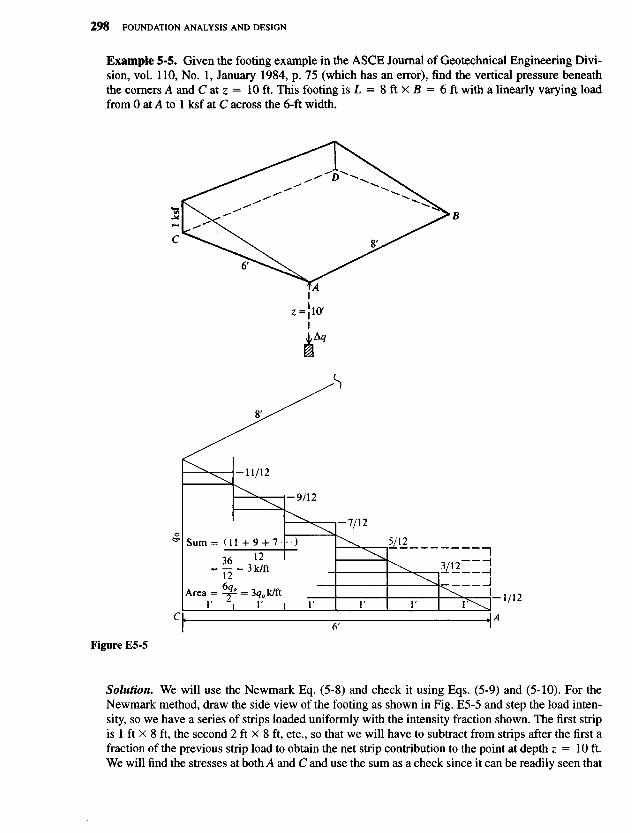
Solution. We will use the Newmark Eq. (5-8) and check it using Eqs. (5-9) and (5-10). For theNewmark method, draw the side view of the footing as shown in Fig. E5-5 and step the load inten-sity, so we have a series of strips loaded uniformly with the intensity fraction shown. The first stripis 1 ft X 8 ft, the second 2 ft X 8 ft, etc., so that we will have to subtract from strips after the first afraction of the previous strip load to obtain the net strip contribution to the point at depth z = 10 ft.We will find the stresses at both A and C and use the sum as a check since it can be readily seen that
Figure E5-5
Example 5-5. Given the footing example in the ASCE Journal of Geotechnical Engineering Divi-sion, vol. 110, No. 1, January 1984, p. 75 (which has an error), find the vertical pressure beneaththe corners A and C at z = 10 ft. This footing is L = 8 ft X B — 6 ft with a linearly varying loadfrom 0 at A to 1 ksf at C across the 6-ft width.
Sum
Area
Summing, we have at A and C = 0.055 56 + 0.069 13 = 0.124 69 ksf. A uniform load of 1 ksf gives Lqa = A#c = 0.1247 ksf basedon Table 5-1 at M = 0.6, N = 0.8. Using Eq. (5-9), we have RD = 14.14;/?| = 136; /?J = 164 and by substitution of values we obtainA^ = 0.055 36 ksf for point A and 0.069 33 ksf for point C.
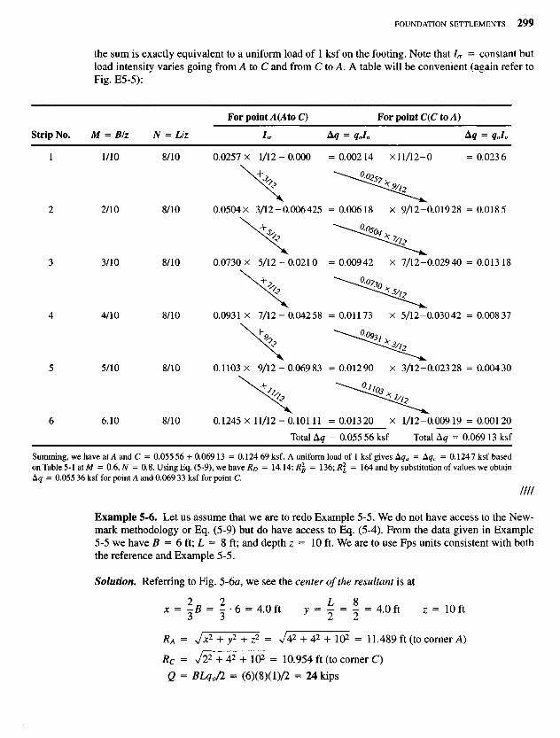
Example 5-6. Let us assume that we are to redo Example 5-5. We do not have access to the New-mark methodology or Eq. (5-9) but do have access to Eq. (5-4). From the data given in Example5-5 we have B = 6 ft; L = 8 ft; and depth z = 10 ft. We are to use Fps units consistent with boththe reference and Example 5-5.
Solution. Referring to Fig. 5-6a, we see the center of the resultant is at
x = \B = \ - 6 = 4.0 ft y = ^ = 5 = 4.0 ft z = 10 ft
RA = Jx1 + v2 + z2 = V42 + 42 + 102 = 11.489 ft (to corner A)
the sum is exactly equivalent to a uniform load of 1 ksf on the footing. Note that Ia = constant butload intensity varies going from A to C and from C to A. A table will be convenient (again refer toFig. E5-5):
1
2
3
4
5
6
1/10
2/10
3/10
4/10
5/10
6.10
8/10
8/10
8/10
8/10
8/10
8/10
Strip No. M = BIz N = Liz
For point A(AtO C) For point C(C to A)
From Eq. (5-4) we have
= 3&L
Separating terms and computing 3QZ3/2TT, we find
3 - 2 ^ 1 0 3 = n 459.129
qvA = 11459.129/11.4895 = 0.0572 ksf
qvC = 11459.129/10.9545 = 0.0727 ksi
The results from Example 5-5 and this example are next compared:
Refer to Table E5-6 for a complete comparison of pressure profiles. For the computationalpurist some of the differences shown in Table E5-6 are substantial, but may be adequate—evenconservative—for design purposes in an engineering office—and certainly the point load equation[Eq. (5-4)] is the easiest of all methods to use.
TABLE E5-6Comparison of stress values from the Boussinesq point loadequation (Eq. 5-4) and Eq. (5-4) converted to a numerical formatusing program SMBWVPRefer to example Fig. E5-5 for location of points A and C.
10.0t 0.0572 0.0727 0.0555 0.069112.0 0.0482 0.0575 0.0463 0.054614.0 0.0401 0.0459 0.0384 0.043716.0 0.0333 0.0371 0.0321 0.035518.0 0.0279 0.0304 0.0270 0.0293*Not from computations but known value.
tDepth used in Examples 5-5 and 5-6.
i SIMPLE METHOD FOR ALL SPECIAL LOADING CASES. Example 5-6 illustrates that/hen the load pattern is difficult (for example, a base covered with an uneven pile of material
producing a nonuniform load), the following procedure is adequate for design:
1. Locate the load resultant as best you can so critical footing locations such as corners, thecenter, and so forth can be located using JC, y coordinates with respect to the load resultant.
2. For the case of depth z = 0, use the computed contact pressure as your best estimate. Youmust do this since z — 0 computes a value of qv = 0 or undefined (o°) in Eq. (5-4).
3. For depth z > 0 compute the value R and use Eq. (5-4). For cases where R < z, Eq. (5-4)will not give very good values but may be about the best you can do. In Example 5-6 notethat R is not much greater than z, but the answers compare quite well with the knownvalues.
4. Consider using Table E5-6 as a guide to increase proportionately your Boussinesq pres-sures, as computed by Eq. (5-4), to approximate more closely the "exact" pressure valuesobtained by the numerical method. For example you actually have an R = 2.11 m (whichcorresponds exactly to the 4.0 ft depth on Table E5-6, so no interpolation is required), andyou have a computed gy,Comp = 9.13 kPa at point A. The "corrected" (or at least morenearly correct) qv can be computed as follows:
_ gu.nmqv — A </i;,comp
<lv,b
where qv,nm = vertical pressure from numerical method (most correct)
qv,b = vertical pressure from Boussinesq Eq. (5-4)
so in our case above, we have
qv = J j ^ X 9.13 = 1.54 x 9.13 = 14.13 kPa
Pressures at other depth points would be similarly scaled. You might note that at the depthof 3.05 m (10 ft) the ratio is 0.0555/0.0572 = 0.970 at point A.
5-5 WESTERGAARD'S METHOD FOR COMPUTINGSOIL PRESSURES
When the soil mass consists of layered strata of fine and coarse materials, as beneath a roadpavement, or alternating layers of clay and sand, some authorities are of the opinion theWestergaard (1938) equations give a better estimate of the stress qv.
The Westergaard equations, unlike those of Boussinesq, include Poisson's ratio /JL, and thefollowing is one of several forms given for a point load Q:
- Q J" << \%\qv
2TTZ2 [a + (r/z)2]3^1 K }
where a = (1 - 2/z,)/(2 - 2/JL) and other terms are the same as in the Boussinesq equation.We can rewrite this equation as
(5-13«)
as done for the Boussinesq equation. For JJL = 0.30 we obtain the following values:
Comparing the Boussinesq values A\, from Eq. (5-5), we see that generally the Westergaardstresses will be larger. This result depends somewhat on Poisson's ratio, however, since /JL =0 and r/z = 0.0 gives Aw = 0.318 (versus Ab = 0.477); for/x = 0.25 and r/z = 0.0 obtainAw = 0.477.
Similarly as for the Boussinesq equation [Eq. (a) and using Fig. 5-2b] we can write
After integration we have the direct solution for round footings analogous to Eq. (5-6):
«-«•('- 7«^;) <5-14)From some rearranging and using the (+) root,
r _ I a 7 ~
z " WO"?/?*)2 a
If this equation is solved for selected values of Poisson's ratio and incremental quantitiesof q/qo, as was done with the Boussinesq equation, values to plot a Westergaard influencechart may be computed. Since the Westergaard equation is not much used, construction of aninfluence chart (done exactly as for the Boussinesq method but for a given value of /x) is leftas an exercise for the reader.
If use of the Westergaard equations is deemed preferable, this is an option programmedinto SMBWVP on your diskette. For programming, the integration of stresses for a rectangleof B X L gives the following equation [used by Fadum (1948) for his stress charts] for thecorner of a rectangular area (and programmed in SMNMWEST) as
where M, Af are previously defined with Eq. (5-8) and a has been defined with Eq. (5-13).The tan"1 term is in radians. This equation can be readily used to obtain a vertical stressprofile as for the Boussinesq equation of Eq. (5-8) for rectangular and round (converted toequivalent square) footings. To check programming, use the following table of values:
M M N Ia
0.45 1.0 1.0 0.18450.45 1.0 0.5 0.1529
At z = 0 we have a discontinuity where we arbitrarily set Ag = qo for any base-on-groundlocation.
5-6 IMMEDIATE SETTLEMENT COMPUTATIONS
The settlement of the corner of a rectangular base of dimensions B' X L' on the surface ofan elastic half-space can be computed from an equation from the Theory of Elasticity [e.g.,Timoshenko and Goodier (1951)] as follows:
A / , ^ i _ ^ ( , + l^,2) ; f 05.1«
where qo = intensity of contact pressure in units of Es
B1 = least lateral dimension of contributing base area in units of AHIi = influence factors, which depend on L'/B\ thickness of stratum H, Poisson's
ratio /i, and base embedment depth DESf /Ji = elastic soil parameters—see Tables 2-7, 2-8, and 5-6
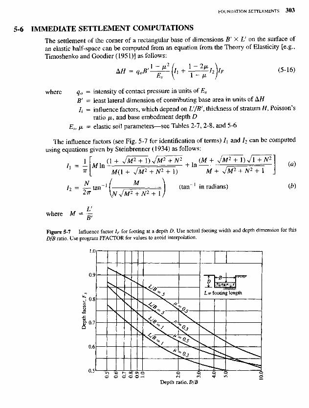
The influence factors (see Fig. 5-7 for identification of terms) h and I2 can be computedusing equations given by Steinbrenner (1934) as follows:
i [ , (i+ JM2+ I)JM2+ N2 _ (M+ VM2 + I )VI+A^ 2 ]Ix = — M In , =— + In - = = = = = = — ya)
IT I M(I + VM2 + W2 + 1) M + VM2 + N2 + 1
I2 = —tan"1 ( M I (tan"1 in radians) (b)2^ \N JM2 + N2 + i /
Vwhere M = -
Figure 5-7 Influence factor IF for footing at a depth D. Use actual footing width and depth dimension for thisDlB ratio. Use program FFACTOR for values to avoid interpolation.
Depth ratio, DfB
Dep
th f
acto
r, F
3 footing length
TABLE 5-2Values of I\ and /2 to compute the Steinbrenner influence factor Is for usein Eq. (5-16a) for several N = HIB' and M = LIB ratios
0.2
0.4
0.6
0.8
1.0
1.5
2.0
3.0
4.0
5.0
6.0
7.0
8.0
9.0
10.0
20.0
500.0
M = 1.0
Z1 = 0.009I2 = 0.041
0.0330.066
0.0660.079
0.1040.083
0.1420.083
0.2240.075
0.2850.064
0.3630.048
0.4080.037
0.4370.031
0.4570.026
0.4710.022
0.4820.020
0.4910.017
0.4980.016
0.5290.008
0.5600.000
1.1
0.0080.042
0.0320.068
0.0640.081
0.1020.087
0.1400.088
0.2240.080
0.2880.069
0.3720.052
0.4210.041
0.4520.034
0.4740.028
0.4900.024
0.5020.022
0.5110.019
0.5190.017
0.5530.009
0.5870.000
1.2
0.0080.042
0.0310.069
0.0630.083
0.1000.090
0.1380.091
0.2240.084
0.2900.074
0.3790.056
0.4310.044
0.4650.036
0.4890.031
0.5060.027
0.5190.023
0.5290.021
0.5370.019
0.5750.010
0.6120.000
1.3
0.0080.042
0.0300.070
0.0610.085
0.0980.093
0.1360.095
0.2230.089
0.2920.078
0.3840.060
0.4400.048
0.4770.039
0.5020.033
0.5200.029
0.5340.025
0.5450.023
0.5540.020
0.5950.010
0.6350.000
1.4
0.0080.042
0.0290.070
0.0600.087
0.0960.095
0.1340.098
0.2220.093
0.2920.083
0.3890.064
0.4480.051
0.4870.042
0.5140.036
0.5330.031
0.5490.027
0.5600.024
0.5700.022
0.6140.011
0.6560.000
1.5
0.0080.042
0.0280.071
0.0590.088
0.0950.097
0.1320.100
0.2200.096
0.2920.086
0.3930.068
0.4550.054
0.4960.045
0.5240.038
0.5450.033
0.5610.029
0.5740.026
0.5840.023
0.6310.012
0.6770.000
1.6
0.0070.043
0.0280.071
0.0580.089
0.0930.098
0.1300.102
0.2190.099
0.2920.090
0.3960.071
0.4600.057
0.5030.048
0.5340.040
0.5560.035
0.5730.031
0.5870.028
0.5970.025
0.6470.013
0.6960.001
1.7
0.0070.043
0.0270,072
0.0570.090
0.0920.100
0.1290.104
0.2170.102
0.2920.094
0.3980.075
0.4650.060
0.5100.050
0.5420.043
0.5660.037
0.5840.033
0.5980.029
0.6100.027
0.6620.013
0.7140.001
1.8
0.0070.043
0.0270.072
0.0560.091
0.0910.101
0.1270.106
0.2160.105
0.2910.097
0.4000.078
0.4690.063
0.5160.053
0.5500.045
0.5750.039
0.5940.035
0.6090.031
0.6210.028
0.6770.014
0.7310.001
1.9
0.0070.043
0.0270.073
0.0560.091
0.0900.102
0.1260.108
0.2140.108
0.2900.100
0.4010.081
0.4730.066
0.5220.055
0.5570.047
0.5830.041
0.6020.036
0.6180.033
0.6310.030
0.6900.015
0.7480.001
2.0
0.0070.043
0.0270.073
0.0550.092
0.0890.103
0.1250.109
0.2130.110
0.2890.102
0.4020.084
0.4760.069
0.5260.058
0.5630.050
0.5900.043
0.6110.038
0.6270.034
0.6410.031
0.7020.016
0.7630.001
TABLE 5-2Values of l\ and h to compute the Steinbrenner influence factor Is for usein Eq. (5-16a) for several N = HIB' and M = LIB ratios (continued)
N
0.2
0.4
0.6
0.8
1.0
1.5
2.0
3.0
4.0
5.0
6.0
7.0
8.0
9.0
10.0
20.0
500.0
M = 2.5
I1 = 0.007I2 = 0.043
0.0260.074
0.0530.094
0.0860.107
0.1210.114
0.2070.118
0.2840.114
0.4020.097
0.4840.082
0.5530.070
0.5850.060
0.6180.053
0.6430.047
0.6630.042
0.6790.038
0.7560.020
0.8320.001
4.0
0.0060.044
0.0240.075
0.0510.097
0.0820.111
0.1150.120
0.1970.130
0.2710.131
0.3920.122
0.4840.110
0.5540.098
0.6090.087
0.6530.078
0.6880.071
0.7160.064
0.7400.059
0.8560.031
0.9770.001
5.0
0.0060.044
0.0240.075
0.0500.097
0.0810.112
0.1130.122
0.1940.134
0.2670.136
0.3860.131
0.4790.121
0.5520.111
0.6100.101
0.6580.092
0.6970.084
0.7300.077
0.7580.071
0.8960.039
1.0460.002
6.0
0.0060.044
0.0240.075
0.0500.098
0.0800.113
0.1120.123
0.1920.136
0.2640.139
0.3820.137
0.4740.129
0.5480.120
0.6080.111
0.6580.103
0.7000.095
0.7360.088
0.7660.082
0.9250.046
1.1020.002
7.0
0.0060.044
0.0240.076
0.0500.098
0.0800.113
0.1120.123
0.1910.137
0.2620.141
0.3780.141
0.4700.135
0.5430.128
0.6040.120
0.6560.112
0.7000.104
0.7370.097
0.7700.091
0.9450.053
1.1500.002
8.0
0.0060.044
0.0240.076
0.0490.098
0.0800.113
0.1120.124
0.1900.138
0.2610.143
0.3760.144
0.4660.139
0.5400.133
0.6010.126
0.6530.119
0.6980.112
0.7360.105
0.7700.099
0.9590.059
1.1910.003
9.0
0.0060.044
0.0240.076
0.0490.098
0.0790.113
0.1110.124
0.1900.138
0.2600.144
0.3740.145
0.4640.142
0.5360.137
0.5980.131
0.6500.125
0.6950.118
0.7350.112
0.7700.106
0.9690.065
1.2270.003
10.0
0.0060.044
0.0240.076
0.0490.098
0.0790.114
0.1110.124
0.1890.139
0.2590.145
0.3730.147
0.4620.145
0.5340.140
0.5950.135
0.6470.129
0.6920.124
0.7320.118
0.7680.112
0.9770.071
1.2590.003
25.0
0.0060.044
0.0240.076
0.0490.098
0.0790.114
0.1100.125
0.1880.140
0.2570.147
0.3680.152
0.4530.154
0.5220.154
0.5790.153
0.6280.152
0.6720.151
0.7100.149
0.7450.147
0.9820.124
1.5320.008
50.0
0.0060.044
0.0240.076
0.0490.098
0.0790.114
0.1100.125
0.1880.140
0.2560.147
0.3670.153
0.4510.155
0.5190.156
0.5760.157
0.6240.157
0.6660.156
0.7040.156
0.7380.156
0.9650.148
1.7210.016
100.0
0.0060.044
0.0240.076
0.0490.098
0.0790.114
0.1100.125
0.1880.140
0.2560.148
0.3670.154
0.4510.156
0.5190.157
0.5750.157
0.6230.158
0.6650.158
0.7020.158
0.7350.158
0.9570.156
1.8790.031
" B'D
B' = — for center; = B for corner /,-
L' = L/2 for center; = L for corner /,-
The influence factor Ip is from the Fox (19482?) equations, which suggest that the set-tlement is reduced when it is placed at some depth in the ground, depending on Poisson'sratio and L/B. Figure 5-7 can be used to approximate Ip. YOU can also use Table 5-2, whichgives a select range of I\ and /2 values, to compute the composite Steinbrenner influencefactor ls as
Is = h + X~f^h (C)1 - IL
Program FFACTOR (option 6) can be used to obtain both Ip and Is directly; you have only toinput appropriate base dimensions (actual L, B for Ip and B', Il for Is) and Poisson's ratio /JL.
Equation (5-16) can be written more compactly as follows:
^H = 4oB' * mlslp (5-16a)
where Is is defined in Eq. (c) and m = number of corners contributing to settlement AH. Atthe footing center m = 4; at a side m = 2, and at a corner m = 1. Not all the rectangles haveto have the same L'/B' ratio, but for any footing, use a constant depth H.
This equation is strictly applicable to flexible bases on the half-space. The half-space mayconsist of either cohesionless materials of any water content or unsaturated cohesive soils.The soils may be either inorganic or organic; however, if organic, the amount of organicmaterial should be very small, because both E5 and /x are markedly affected by high organiccontent. Also, in organic soils the foregoing equation has limited applicability since secondarycompression or "creep" is usually the predominating settlement component.
In practice, most foundations are flexible. Even very thick ones deflect when loaded bythe superstructure loads. Some theory indicates that if the base is rigid the settlement will beuniform (but may tilt), and the settlement factor Is will be about 7 percent less than computedby Eq. (c). On this basis if your base is "rigid" you should reduce the Is factor by about 7percent (that is, Isr = 0.931IS).
Equation (5-16a) is very widely used to compute immediate settlements. These estimates,however, have not agreed well with measured settlements. After analyzing a number of cases,the author concluded that the equation is adequate but the method of using it was incorrect.The equation should be used [see Bowles (1987)] as follows:
1. Make your best estimate of base contact pressure qo.
2. For round bases, convert to an equivalent square.
3. Determine the point where the settlement is to be computed and divide the base (as in theNewmark stress method) so the point is at the corner or common corner of one or up to 4contributing rectangles (see Fig. 5-7).
TABLE 5-3Comparison of computed versus measured settlement for a number of cases provided by the references cited.
Settlement, in.
MeasuredComputed//IsAp9 ksfEn ksfN or qcDIBLIBBJtHJtReference
1.530.8-0.92.48
10.60.273.9
5.30.50
1.500.243.20
0.33
1.450.672.64
11.70.353.9
5.60.50
1.270.243.25
0.75
0.870.751.00.980.60.95
1.00.93
1.01.01.0
0.589
0.8050.7740.500.3490.510.152
0.2550.472
0.1610.4930.483
3.4
3.743.341.564.142.287.2
3.147.0
4.52.754.0
0.33
0.40.30.450.30.30.3
0.30.45
0.30.30.3
1,200
310620350.230110270
39058200
1,1003,900
260
25*
4012065901812*
12-30*
50
0.5
0.78100.10.550.1
00.2
000
1.6
8.84.21.02.21.01.1
11
111
12.5
8.59.8
62872
90
124500
1773220
AB
5B5B5B
B5B0.8 B
901700
150AB3.5B
D'Appoloniaet al.(1968)
Schmertmann(1970)CaselCase 2Case 5Case 6Case 8
Tschebotarioff(1973)Davisson and Salley
(1972)Fischer etal. (1972)Webb and Melvill
(1971)Swiger(1974)Kantey(1965)
Units: Used consistent with references.
*N value, otherwise is qc. Values not shown use other methods for Es.
Source: Bowles (1987).
4. Note that the stratum depth actually causing settlement is not at H/B —> °°, but is at eitherof the following:a. Depth z — 5B where B = least total lateral dimension of base.b. Depth to where a hard stratum is encountered. Take "hard" as that where E8 in the hard
layer is about XQE8 of the adjacent upper layer.
5. Compute the H/B' ratio. For a depth H = z = 5B and for the center of the base we haveH/B1 = 5B/0.5B = 10. For a corner, using the same H, obtain 5B/B = 5. This computa-tion sets the depth H = z = depth to use for all of the contributing rectangles. Do not use,say, H = 5B = 15 m for one rectangle and H = 5B = 10 m for two other contributingrectangles—use 15 m in this case for all.
6. Enter Table 5-2, obtain I\ and /2, with your best estimate for /UL compute I8, and obtain Iffrom Fig. 5-7. Alternatively, use program FFACTOR to compute these factors.
7. Obtain the weighted average E8 in the depth z = H. The weighted average can be com-puted (where, for n layers, H = 2 " Ht) as
H\ES\ H- H2E& + • • • H- HnE8n
Table 5-3 presents a number of cases reanalyzed by the author using the foregoing pro-cedure. It can be seen that quite good settlement estimates can be made. Earlier estimateswere poor owing to two major factors: One was to use a value of E5 just beneath the baseand the other was to use a semi-infinite half-space so that I8 = 0.56 (but the /2 contributionwas usually neglected—i.e., /x = 0.5). A curve-fitting scheme to obtain I8 used by Gazetaset al. (1985) appeared to have much promise for irregular-shaped bases; however, using themethod for some cases in Table 5-3 produced such poor settlement predictions compared withthe suggested method that these equations and computation details are not recommended foruse. Sufficient computations are given in Bowles (1987) to allow the reader to reproduce Es
and AH in this table.This method for immediate settlements was also used to compute estimated loads for a
set of five spread footings [see Briaud and Gibbens (1994)] for purposes of comparison withreported measured values for a settlement of AH = 25 mm. A substantial amount of datawas taken using the test methods described in Chap. 3, including the SPT, CPT, PMT, DMT,and Iowa stepped blade. For this text the author elected to use only the CPT method with qc
obtained by enlarging the plots, estimating the "average" qc by eye for each 3 m (10 ft) ofdepth, and computing a resulting value using
ZH1
It was reported that the sandy base soil was very lightly overconsolidated so the coneconstant was taken as 5.5 for all footings except the 1 X 1 m one where the size was such thatany soil disturbance would be in the zone of influence. Clearly one can play a numbers gameon the coefficient, however, with 3.5 regularly used for normally consolidated soils and from6 to 30 for overconsolidated soils (refer to Table 5-6), any value from 4 to 7 would appearto apply—5.5 is a reasonable average. With these data and using the program FFACTORon your diskette for the IF and I8 (which were all 0.505, because the bases were square and
TABLE 5-4Comparison of computed versus measured spread footing loads for a 25-mm settlement after30 min of load. Poisson's ratio /t = 0.35 for all cases.
T ^ ^ I I ', I ^ Footing load, kNBXB9 ^,average, Cone E8 = ^,average, FOX pressure Atf,
because we used an effective influence depth of 51?) factors, Table 5-4 was developed. Anyneeded Fps values in the original reference were converted to SI.
Example 5-7. Estimate the settlement of the raft (or mat) foundation for the "Savings Bank Build-ing" given by Kay and Cavagnaro (1983) using the author's procedure. Given data are as follows:
qo = 134 kPa B X L = 33.5 X 39.5 m measured AH = about 18 mmSoil is layered clays with one sand seam from ground surface to sandstone bedrock at- 14 m; mat at - 3 m.
Es from 3 to 6 m = 42.5 MPa Es from 6 to 14 m = 60 MPaEs for sandstone > 500 MPa
Solution. For clay, estimate JJL = 0.35 (reference used 0.2). Compute
3 x 42.5 + 8 x 60£s(average) = y. = 55 MFa
From base to sandstone H = 1 4 - 3 = 11m.
B' = Q* = 16.75 m (for center of mat) -* ~ = - ^ - = 0.66 (use 0.7)2 B lo./j
Interpolating in Table 5-2, we obtain Ix = 0.0815; I2 = 0.086:
/, = 0.0815 + 1~_2(^)3
35) (0.0865) = 0.121
f = 3I5 =0.09; use/F =0.95
With four contributing corners m = 4 and Eq. (5-16a) gives
AH = qoB'l--^AIsIF
A// = 134(16.75)} ~ °;^L(4 X 0.121)(0.95)(1000) = 16.5 mm55 X 1000
(The factor 1000 converts MPa to kPa and m to mm.)
This estimate is rather good when compared to the measured value of 18 mm. If this were madefor a semi-infinite elastic half-space (a common practice) we would obtain (using E5 just underthe mat)
AH = 134 [ 1 6 / 7 5 ( ^ ^ ( 4 X 0.56 X 0.95 X 1000)1 = 98.6 mmL \42 5001 J
which is seriously in error. You should study the reference and these computations to appreciatethe great difficulty in making settlement predictions and then later trying to verify them—evenapproximately.
////
5-7 ROTATIONOFBASES
It is sometimes necessary to estimate the rotation of a base. This is more of a problem withbases subjected to rocking moments producing vibrations (considered in more detail in Chap.20), however, for static rotations as when a column applies an overturning moment it may benecessary to make some kind of estimate of the rotation.
A search of the literature produced five different solutions—none of which agreed wellwith any other—for flexible base rotation under moment. On this basis, and because theo-retical solutions require full contact of base with the soil and with overturning often the fullbase area is not in contact, the best estimate would be made using a finite difference solution.The finite difference solution is recommended since the overturning moment can be modeledusing statics to increase the node forces on the pressed side and decrease the node forceson the tension side. The average displacement profile across the base in the direction of theoverturning effort can be used to obtain the angle of rotation. This computer program is B-19in the package of useful programs for Foundation Design noted on your diskette.
Alternatively, the footing rotation can be expressed (see Fig. 5-8) as
tan* = '-if WZ1* (5"17)
where M = overturning moment resisted by base dimension B. Influence values IQ that maybe used for a rigid base were given by Taylor (1967) as in Table 5-5. Values of IQ for a flexiblebase are given by Tettinek and Matl (1953, see also Frolich in this reference p. 362). Theseflexible values are intermediate to those of several other authorities. The rotation spring of
Figure 5-8 Rotation of a footing on an elas-tic base.
TABLE 5-5
Influence factors I6 to compute rotation of a footing
*For circle B = diameter.tThere are several "rigid" values; these are from equations given by Taylor (1967, Fig. 9, p. 227). Theycompare reasonably well with those given by Poulos and Davis (1974, p. 169, Table 7.3).
Table 20-2 may also be used to compute base rotation. Most practical footings are intermedi-ate between "rigid" and "flexible" and require engineering judgment for the computed valueof footing rotation 6.
Using a computer program such as B19 or the influence factors of Table 5-5 gives a nearlylinear displacement profile across the footing length L. This result is approximately correctand will produce the constant pressure distribution of Fig. 4-4a since the soil will behave sim-ilarly to the compression block zone used in concrete beam design using the USD method.In that design the concrete strains are assumed linear but the compression stress block isrectangular. One could actually produce this case using program B19 (FADMATFD) if thenonlinear switch were activated and the correct (or nearly correct) value of maximum lin-ear soil displacement XMAX were used. Enough concrete beam testing has been done todetermine that the maximum linear strain is approximately 0.003. Finding an XMAX thatwould produce an analogous rectangular pressure profile under the pressed part of a footingundergoing rotation would involve trial and error. Making several runs of program B19 witha different XMAX for each trial would eventually produce a reasonable rectangular pressureprofile, but this is seldom of more than academic interest. The only XMAX of interest in thistype of problem is one that gives
q = XMAX -ks^qa
When this is found the resulting average displacement profile can be used to estimate baseand/or superstructure tilt.
Example 5-8.
Given. A rectangular footing with a column moment of 90 kN • m and P = 500 kN. Footing is3 X 2 X 0.5 m thick. The soil parameters are Es = 10000 kPa, ju, = 0.30. The concrete column is0.42 X 0.42 m and has a length of 2.8 m, and Ec = 27.6 X 10⁶ kPa. Estimate the footing rotation
and find the footing moment after rotation assuming the upper end of the column is fixed as shownin Fig. E5-8.
Solution,
I6 = 2.8 (interpolated from Table 5-5, column "Flexible")
1 - /JL2 M T
tane = -wrwih
1 - 0 3 2 90
tan 0 = 0.001 274 rad
6 = 0.073°
From any text on mechanics of materials the relationship between beam rotation and moment(when the far end is fixed, the induced M' = M/2) is
0~4EI
from which the moment to cause a column rotation of 6 is
U = ^L6JLJ
The column moment of inertia is
7 . £ - A £ - 2 . 5 9 3 x ID-m<
Substitution of/, Ec, L, and 6 gives the released column moment of
M = ^27.6x10^(2.593x10-3X1.274x10-3) =
2.8
Since the rotation is equivalent to applying a moment of 130 kN • m opposite to the given M of90 kN • m, the footing moment is reduced to zero and the base 6 < 0.073°. There is also a changein the "far-end" column moment that is not considered here.