Introduction Fundamentals Dynamic Programming Optimal Control Concluding Remarks Foundations of Dynamic Macroeconomic Analysis Ping Wang, Washington University in St. Louis/NBER January 2018
Transcript
Introduction Fundamentals Dynamic Programming Optimal Control Concluding Remarks
Foundations ofDynamic Macroeconomic Analysis
Ping Wang, Washington University in St. Louis/NBER
January 2018
Introduction Fundamentals Dynamic Programming Optimal Control Concluding Remarks
Introduction
This set of lecture notes provides foundations of macroanalysis, focusing particularly on the following issues:
1 Fundamentals of Dynamic General Equilibrium2 Optimal Growth in Discrete Time3 Optimal Growth in Continuous Time
Basic references:
1 Acemoglu (2009): chs. 5-72 Aghion and Howitt (1998): chs. 1-23 Barro and Sala-i-Martin: ch. 2, secs. 4.1-4.34 Ljungqvist and Sargent (2000): chs. 3 and 115 Stokey and Lucas with Prescott (1989): chs. 3-56 Wang (2012), “Endogenous Growth Theory,” Lecture
Notes, Washington University-St. Louis.
Introduction Fundamentals Dynamic Programming Optimal Control Concluding Remarks
Representative Household I
Representative household is valid when the optimizationof individual households can be represented as if therewere a single household making the aggregate decisionsusing a representative preference subject to aggregateconstraints.Consider a particular preferences representation:
max∞
∑t=0
βtu (c (t))
Let the excess demand of the economy be x(p).Key: whether this excess demand function x(p) can beobtained as a solution to the single household optimizationproblem.
Introduction Fundamentals Dynamic Programming Optimal Control Concluding Remarks
Representative Household II
Answer at the first glance: it cannot be so obtained ingeneral as the weak axiom of revealed preferences forindividuals need not hold for the aggregate.
Theorem H1 (Debreu-Mantel-Sonnenschein Theorem) Letε > 0 and N ∈N. Consider a set of pricesPε = p ∈ RN
+ : pj/pj′ ≥ ε for all j and j′ and any continuous
function x : Pε → RN+ that satisfies Walras’s Law and is
homogeneous of degree 0. Then there exists an exchangeeconomy with N commodities and H < ∞ households, wherethe aggregate excess demand is given by x (p) over the set Pε.
To yield a positive answer ensuring the excess demandfunction x(p) to be obtained as a solution to the singlehousehold optimization problem, we need to imposefurther restrictions, in particular, to remove strong incomeeffects.
Introduction Fundamentals Dynamic Programming Optimal Control Concluding Remarks
Representative Household III
A special but useful case for such a representation is tohave linear value (indirect utility) function:
Theorem H2 (Gorman’s Aggregation Theorem) Consider andeconomy with N < ∞ commodities and a setH of households.Suppose that the preferences of each household h ∈ H can berepresented by an indirect utility function of the form
υh(
p, wh)= ah (p) + b (p)wh
and that each household h ∈ H has a positive demand for eachcommodity. Then these preferences can be aggregated andrepresented by those of a representative household, withindirect utility
υ (p, w) = a (p) + b (p)w,
where a (p) ≡∫
h∈H ah (p) dh, and w ≡∫
h∈H whdh is aggregateincome.
Introduction Fundamentals Dynamic Programming Optimal Control Concluding Remarks
Representative Household IV
The class of preferences described in Theorem H-2 isreferred to as “Gorman preferences” (1959 Econometrica).In this class, the Engel curve of each household for eachcommodity is linear and its slope is identical to allindividuals for the same commodity.By Roy’s Identity,
xhj
(p, wh
)= − 1
b (p)∂ah (p)
∂pj− 1
b (p)∂b (p)
∂pjwh
Therefore, for each household, a linear relationship existsbetween demand and income and the slope, − 1
b(p)∂b(p)
∂pj, is
independent of the household’s identity (h).
Introduction Fundamentals Dynamic Programming Optimal Control Concluding Remarks
Representative Household V
Even under class of “Gorman preferences” a representativehousehold exists, typical macro models require furtherrestrictions on:
the abstract of distribution effects from the representativehousehold’s concern (strong representation);the use of the representative household’s preference as thewelfare function of the aggregate economy (normativerepresentation).
Introduction Fundamentals Dynamic Programming Optimal Control Concluding Remarks
Representative Household VI
Normative representation requires convexity, interiorityand price-invariant basic value (o.w., one can transfer εfrom low to high-valuation households for different p):
Theorem H3 (Normative Representation) Consider aneconomy with a finite number N < ∞ of commodities, a setHof households, and a convex aggregate production possibilitiesset Y. Suppose that the preferences of each household h ∈ H isrepresented by υh (p, wh) = ah (p) + b (p)wh withp = (p1, ..., pN) and that each household h ∈ H has a positivedemand for each commodity.1. Then any feasible allocation that maximizes the utility of therepresentative household υ (p, w) = ∑h∈H ah (p) + b (p)w, withw ≡ ∑h∈H wh, is Pareto optimal.2. If ah (p) = ah for all p and all h ∈ H (price-invariant basicvalue), then any Pareto optimal allocation maximizes the utilityof the representative household.
Introduction Fundamentals Dynamic Programming Optimal Control Concluding Remarks
Representative Firm I
Representative firm is valid when the optimization ofindividual firms can be represented as if there were asingle firm making the aggregate decisions using anaggregate production function subject to aggregateconstraints.Consider price and output vectors: p = (p1, ..., pN) andy = (y1, ..., yN), with p · y = ∑N
j=1 pjyj.Let F be the countable set of firms in the economy and
Y ≡
∑f∈F
yf : yf ∈ Yf for each f ∈ F
be the aggregate production possibility set (PPS).
Introduction Fundamentals Dynamic Programming Optimal Control Concluding Remarks
Representative Firm II
When there is no price-dependent fixed cost (ensuredunder perfect competition in the absence of externalities),we have:
Theorem F (Representative Firm Theorem) Consider acompetitive production economy with N ∈N∪ +∞commodities and a countable set F of firms, each with aproduction possibilities set Yf ⊂ RN. Let p ∈ RN
+ be the pricevector in this economy and denote the set of profit-maximizingnet supplies of firm f ∈ F by Yf (p) ⊂ Yf so that for anyyf ∈ Yf (p), we have p · yf ≥ p · yf for all yf ∈ Yf . Then thereexists a representative firm with production possibilities setY ⊂ RN and a set of profit-maximizing net supplies Y (p) suchthat for any p ∈ RN
+, y ∈ Y (p) if and only if y = ∑f∈F yf forsome yf ∈ Yf (p) for each f ∈ F .
Introduction Fundamentals Dynamic Programming Optimal Control Concluding Remarks
Equilibrium
An economy E is described by preferences, endowments,production sets, consumption sets, and allocation ofshares, that is, E ≡ (H,F , U, ω, Y, X, θ).An allocation (x, y) in E , x ∈ X, y ∈ Y, is feasible if∑h∈H xh
j ≤ ∑h∈H ωhj +∑f∈F yf
j for all j ∈N.
Definition E (Competitive Equilibrium) A competitiveequilibrium for economy E ≡ (H,F , U, ω, Y, X, θ) is given by afeasible allocation
(x∗ = xh∗h∈H, y∗ = yf∗f∈F
)and a price
system p∗ such that1. (Firm optimization) For every firm f ∈ F , yf∗ maximizesprofits: p∗ · yf∗ ≥ p∗ · yf for all yf ∈ Yf .2. (Household optimization) For every household h ∈ H, xh∗
maximizes utility: Uh (xh∗) ≥ Uh (xh) for all x such that xh ∈ Xh
and p∗ · xh ≤ p∗(
ωh +∑f∈F θhf yf)
.
Introduction Fundamentals Dynamic Programming Optimal Control Concluding Remarks
Pareto Optimum
The standard concept of optimality is Pareto optimum,though social optimum is often used in macroeconomics.
Definition O (Pareto Optimum) A feasible allocation (x, y) foreconomy E ≡ (H,F , U, ω, Y, X, θ) is Pareto optimal if thereexists no other feasible allocation (x′, y′) such that x′h ∈ Xh forall h ∈ H, y′f ∈ Yf for all f ∈ F , and Uh (x′h) ≥ Uh (xh) for all
h ∈ H with Uh′(
x′h′)> Uh′
(xh′)
for at least one h′ ∈ H.
Introduction Fundamentals Dynamic Programming Optimal Control Concluding Remarks
Welfare Theorems I
Household h ∈ H is locally nonsatiated if, at each xh ∈ Xh,Uh (xh) is strictly increasing in at least one of its argumentsand Uh (xh) < ∞.
Theorem W1 (First Welfare Theorem I) Suppose that(x∗, y∗, p∗) is a competitive equilibrium of economyE ≡ (H,F , U, ω, Y, X, θ) withH finite. Assume continuouspreferences with all households locally nonsatiated. Then(x∗, y∗) is Pareto optimal (PO).Theorem W2 (First Welfare Theorem II) Suppose that(x∗, y∗, p∗) is a competitive equilibrium of economyE ≡ (H,F , U, ω, Y, X, θ) withH countably infinite. Assumecontinuous preferences with all households locally nonsatiatedand
p∗ ·ω∗ ≡ ∑h∈H
∞
∑j=0
p∗j ωhj < ∞.
Then (x∗, y∗, p∗) is Pareto optimal.
Introduction Fundamentals Dynamic Programming Optimal Control Concluding Remarks
Welfare Theorems II
Theorem W3 (Second Welfare Theorem) Consider a Paretooptimal allocation (x∗, y∗) in an economyE ≡ (H,F , U, ω∗, Y, X, θ∗). Suppose that all consumption setsare convex, all production sets are convex cones, all utilityfunctions are continuous and quasi-concave, and interiorityconditions are met such that (i) there exists χ < ∞ such that∑h∈H xh
j,t < χ for all j and t; (ii) 0¯∈ Xh for each h; (iii) for any h
and xh, xh ∈ Xh such that Uh (xh) > Uh (xh), there existsT(h, xh, xh) such that Uh (xh [T]
)> Uh (xh) for all
T ≥ T(h, xh, xh); and (iv) for any f and yf ∈ Yf , there existsT(f , yf ) such that yf [T] ∈ Yf for all T ≥ T(f , yf ). Then thereexists a price vector p∗ and endowment and share allocations(ω∗, θ∗) with ω∗ = ∑h∈H ωh∗, θ∗ = ∑f∈F θf∗, such that:1. for all f ∈ F , p∗ · yf∗ ≥ p∗ · yf for any yf ∈ Yf ;2. for all h ∈ H, if Uh (xh) > Uh (xh∗) for some xh ∈ Xh thenp∗ · xh ≥ p∗ ·wh∗, where wh∗ ≡ ωh∗ +∑f∈F θf∗yf∗.
Introduction Fundamentals Dynamic Programming Optimal Control Concluding Remarks
Welfare Theorems III
The Second Welfare Theorem can be readily used to provethe existence of a competitive equilibrium based onBrouwer/Kakutani.
Theorem W3 (Existence of Competitive Equilibrium)Consider an economy E as described in Theorem W3, ifp∗ ·wh∗ > 0 for each h ∈ H, then there exists a competitiveequilibrium (x∗, y∗, p∗).
Introduction Fundamentals Dynamic Programming Optimal Control Concluding Remarks
Dynamic General Equilibrium I
To generalize the standard Arrow-Debreu-McKenzeigeneral equilibrium (GE) analysis to an infinite-horizondynamic framework (DGE), one needs to impose furtherrestrictions, particularly in the following aspects:
finite value: bounded valuation of households/firmsinfinite dimensional space: Banach Space, Hilbert Space,Polish Space with weak or weak* topology rather thanstandard product topologyinfinite dimensional fixed point: Schauder and othersinteriority in infinite dimensioninformation and Arrow-Debreu trade.
Introduction Fundamentals Dynamic Programming Optimal Control Concluding Remarks
Dynamic General Equilibrium II
In the context of optimal growth, such DGE frameworksare given by
s.t. yt ∈ G(t, xt) ∀t ≥ 0xt+1 = f (t, xt, yt) ∀t ≥ 0x0 > 0 given
Eliminate yt and rewrite the optimization problem:
V∗0 (x0) = supxt∞t=0
∑∞t=0 βtUt(xt, xt+1)
s.t. xt+1 ∈ Gt(t, xt) ∀t ≥ 0x0 > 0 given.
Introduction Fundamentals Dynamic Programming Optimal Control Concluding Remarks
Dynamic Programming II
Under stationarity, Ut = U and Gt = G, yielding thefollowing recursive problem:
V∗(x0) = supxt∞t=0
∑∞t=0 βtU(xt, xt+1)
s.t. xt+1 ∈ G(xt) ∀t ≥ 0x0 given
The functional problem is (Bellman equation):
V(x) = supy∈G(x)
U(x, y) + βV(y) ∀x ∈ X.
Introduction Fundamentals Dynamic Programming Optimal Control Concluding Remarks
Dynamic Programming III
Feasible set:Φ(xt) = xs∞
s=t : xs+1 ∈ G(xs), s = t, t+ 1, ....Let X be a compact subset of RK andXG = (x, y) ∈ X×X : y ∈ G(x).Assumption A1:
(a) G(x) 6= ∅ for all x ∈ X;(b) G is compact-valued and continuous;(c) G is an increasing set s.t. x ≤ x′ ⇒ G(x) ⊂ G(x′).
Assumption A2:(a) ∀ x0 ∈ X and x ∈ Φ(x0),limn→∞ ∑n
t=0 βtU(xt, xt+1) = V∞ < ∞;(b) U : XG → R is continuous;(c) U(x, y) is strictly increasing in the first K elements foreach y ∈ X;(d) U(x, y) is strictly concave in (x, y);(e) U is continuously differentiable over intXG.
Introduction Fundamentals Dynamic Programming Optimal Control Concluding Remarks
Dynamic Programming IV
Applying sandwich theorem, we can show:
Theorem DP1 (Equivalence of Values) Under A1(a) and A2(a),the solution to the recursive problem V∗(x0) is equivalent to thesolution to the functional problem V(x), i.e., V∗(x) = V(x) forall x ∈ X.
By recursive substitution, it is straightforward to obtain:
Theorem DP2 (Principle of Optimality) Under A1(a) andA2(a), consider a feasible plan x∗ ∈ Φ(x0) that attains V∗(x0) inthe recursive problem. Then
V∗(x∗t ) = U(x∗t , x∗t+1) + βV∗(x∗t+1)
for t = 0, 1, ... with x∗0 = x0. Moreover, if any x∗ ∈ Φ(x0) attainsV(x) in the functional problem, then it attains the optimal valuein the recursive problem.
Introduction Fundamentals Dynamic Programming Optimal Control Concluding Remarks
Dynamic Programming V
With continuity as well as compactness of the constraintset, we can apply Beige’s Theorem of Maximum andWeierstrass Theorem to obtain:
Theorem DP3 (Existence of Solutions) Under A1(a,b) andA2(a,b), there exists a unique continuous and boundedfunction V : X→ R that satisfies the Bellman equation.Moreover, for any x0 ∈ X, an optimal plan x∗ ∈ Φ(x0) exists.
With concavity and differentiability, we have:
Theorem DP4 (Differentiability of the Value Function) UnderA1(a,b) and A2(a,b,d,e), consider an optimal plan x∗ and defineπ as the policy function satisfying x∗t+1 = π(x∗t ). Furtherassume that x ∈ intX and π(x) ∈ intG(x). Then V(·) isdifferentiable at x, with gradient DV(x) = DxU(x, π(x)).
Introduction Fundamentals Dynamic Programming Optimal Control Concluding Remarks
Dynamic Programming VI
Let (s, d) be a norm space and T : S→ S be an operatormapping S into itself. If for some β ∈ (0, 1),
d(Tz1, Tz2) ≤ βd(z1, z2) ∀z1, z2 ∈ S
Then T is a contraction mapping (with modulus β).
Theorem DP5 (Contraction Mapping Theorem) Let (s, d) be acomplete norm space and suppose that T : S→ S is acontraction. Then T has a unique fixed point, z, i.e., there existsa unique z ∈ S such that Tz = z.
Introduction Fundamentals Dynamic Programming Optimal Control Concluding Remarks
Dynamic Programming VII
In practice, the following theorem provide sufficientconditions for a contraction map:
Theorem DP6 (Blackwell’s Sufficient Conditions for aContraction) Let X ⊆ Rk, and B(X) be the space of boundedfunctions f : X→ R defined on X equipped with the sup norm|| · ||. Suppose that B′(X) ⊂ B(X), and let T : B′(X)→ B′(X) bean operator satisfying the following two conditions:1. (Monotonicity) For any f , g ∈ B′(X), f (x) ≤ g(x) ∀x ∈ X,(Tf )(x) ≤ (Tg)(x) ∀x ∈ X;2. (Discounting) ∃ β ∈ (0, 1) s.t. [T(f + c)](x) ≤ (Tf )(x) + βc∀f ∈ B(X), c ≥ 0, and x ∈ X.Then T is a contraction (with modulus β) on B′(X).
Introduction Fundamentals Dynamic Programming Optimal Control Concluding Remarks
Dynamic Programming VIII
Applying Contraction Mapping Theorem to the valuefunction V, we can establish its properties:
Theorem DP7 (Value Function Properties) Under A1(a,b,c)and A2(a,b,c,d), V(x) in the Bellman equation is strictlyincreasing in all of its arguments and strictly concave.Theorem DP8 (Necessity and Sufficiency) Under A1(a,b,c)and A2(a,b,c,d,e), a sequence x∗t ∞
t=0 such that x∗t+1 ∈ intG(x∗t ),t = 0, 1..., is optimal for the recursive problem given x0 if andonly if it satisfies the following:1. (Euler Equations) DyU(x, π(x)) + βDxU(π(x), π(π(x))) = 02. (Transversality Conditions) limt→∞ βtDxU(x∗, x∗t+1)x
∗t = 0.
Introduction Fundamentals Dynamic Programming Optimal Control Concluding Remarks
Dynamic Programming IX
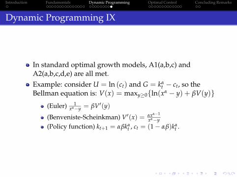
In standard optimal growth models, A1(a,b,c) andA2(a,b,c,d,e) are all met.Example: consider U = ln (ct) and G = kα
t − ct, so theBellman equation is: V(x) = maxy≥0ln(xα − y) + βV(y)
(Euler) 1xα−y = βV′(y)
(Benveniste-Scheinkman) V′(x) = αxα−1
xα−y(Policy function) kt+1 = αβkα
t , ct = (1− αβ)kαt .
Introduction Fundamentals Dynamic Programming Optimal Control Concluding Remarks
Optimal Control I
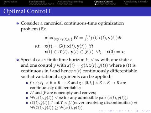
Consider a canonical continuous-time optimizationproblem (P):
Special case: finite time horizon t1 < ∞ with one state xand one control y with ˙x(t) = g(t, x(t), y(t)) where y (t) iscontinuous in t and hence x(t) continuously differentiableso that variational arguments can be applied:
f : [0, t1]× R× R→ R and g : [0, t1]× R× R→ R arecontinuously differentiable;X and Y are nonempty and convex;W(x(t), y(t)) < ∞ for any admissible pair (x(t), y(t));(x(t), y(t)) ∈ intX ×Y (never involving discontinuities)⇒W(x(t), y(t)) ≥ W(x(t), y(t)).
Introduction Fundamentals Dynamic Programming Optimal Control Concluding Remarks
Introduction Fundamentals Dynamic Programming Optimal Control Concluding Remarks
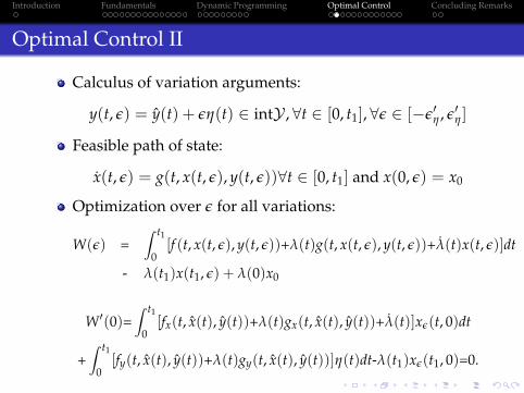
Optimal Control III
Theorem OC1 (Necessary Conditions) Consider the problem(P) with t1 < ∞, one state-one control and f and g continuouslydifferentiable. Suppose that (P) has an interior continuoussolution (x(t), y(t)) ∈ intX ×Y . Then there exists acontinuously differentiable costate function λ(·) defined ont ∈ [0, t1] such that:
(Complementary slackness) λ(t1)(x(t1)− x1) = 0 ifx(t1) ≥ x1, with λ(t1) > 0 if x(t1) = x1.If t1 is given (as is x(t1) = x1), then there is no need forλ(t1) = 0.
Introduction Fundamentals Dynamic Programming Optimal Control Concluding Remarks
Optimal Control IV
Hamiltonian (which is continuously differentiable as well):H(t, x(t), y(t), λ(t)) = f (t, x(t), y(t)) + λ(t)g(t, x(t), y(t)).
Theorem OC2 (Maximum Principle) Consider (P) given inTheorem OC1. Suppose that (P) has an interior continuoussolution (x(t), y(t)) ∈ intX ×Y . Then there exists acontinuously differentiable function λ(t) such that the optimalcontrol y(t) and the corresponding path of the state variablex(t) satisfy the following necessary conditions (NC):
with x(0) = x0 and λ(t1) = 0. Moreover, H(t, x, y, λ) alsosatisfies the Maximum Principle:H(t, x(t), y(t), λ(t)) ≥ H(t, x(t), y, λ(t)), ∀y ∈ Y , ∀t ∈ [0, t1].
Introduction Fundamentals Dynamic Programming Optimal Control Concluding Remarks
Optimal Control V
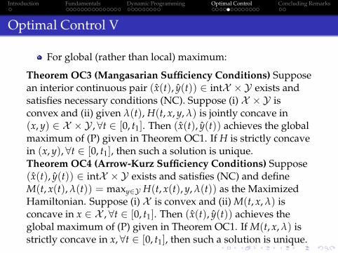
For global (rather than local) maximum:
Theorem OC3 (Mangasarian Sufficiency Conditions) Supposean interior continuous pair (x(t), y(t)) ∈ intX ×Y exists andsatisfies necessary conditions (NC). Suppose (i) X ×Y isconvex and (ii) given λ(t), H(t, x, y, λ) is jointly concave in(x, y) ∈ X ×Y , ∀t ∈ [0, t1]. Then (x(t), y(t)) achieves the globalmaximum of (P) given in Theorem OC1. If H is strictly concavein (x, y), ∀t ∈ [0, t1], then such a solution is unique.Theorem OC4 (Arrow-Kurz Sufficiency Conditions) Suppose(x(t), y(t)) ∈ intX ×Y exists and satisfies (NC) and defineM(t, x(t), λ(t)) = maxy∈Y H(t, x(t), y, λ(t)) as the MaximizedHamiltonian. Suppose (i) X is convex and (ii) M(t, x, λ) isconcave in x ∈ X , ∀t ∈ [0, t1]. Then (x(t), y(t)) achieves theglobal maximum of (P) given in Theorem OC1. If M(t, x, λ) isstrictly concave in x, ∀t ∈ [0, t1], then such a solution is unique.
Introduction Fundamentals Dynamic Programming Optimal Control Concluding Remarks
Optimal Control VI
We now generalize the theorems to the multivariate case:
Theorem OC5 (Maximum Principle) Consider (P) with t1 < ∞and f and g continuously differentiable. Suppose it has aninterior continuous solution (x(t), y(t)) ∈ intX ×Y and defineH(t, x, y, λ) = f (t, x(t), y(t)) + λ(t) ·G(t, x(t), y(t)), λ(t) ∈ RKx .Then (x(t), y(t)) satisfy the following necessary conditions:
If X is convex and M(t, x, λ) = maxy(t)∈Y H(t, x(t), y, λ(t)) isconcave in x ∈ X , ∀t ∈ [0, t1], then (x(t), y(t)) achieves theglobal maximum of (P) given above. If M(t, x, λ) is strictlyconcave in x, ∀t ∈ [0, t1], then such a solution is unique.
Introduction Fundamentals Dynamic Programming Optimal Control Concluding Remarks
Optimal Control VII
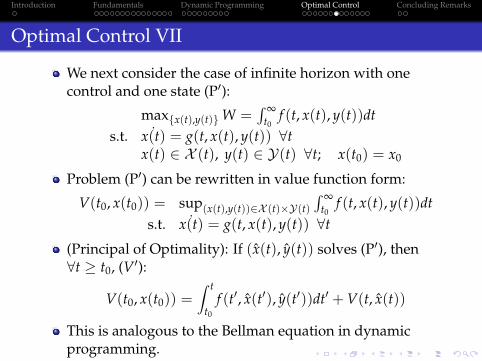
We next consider the case of infinite horizon with onecontrol and one state (P′):
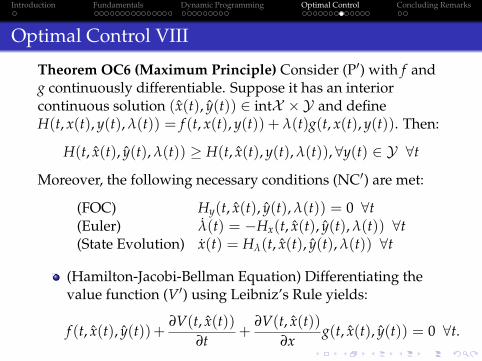
(Hamilton-Jacobi-Bellman Equation) Differentiating thevalue function (V′) using Leibniz’s Rule yields:
f (t, x(t), y(t))+∂V(t, x(t))
∂t+
∂V(t, x(t))∂x
g(t, x(t), y(t)) = 0 ∀t.
Introduction Fundamentals Dynamic Programming Optimal Control Concluding Remarks
Optimal Control IX
Sufficiency conditions ensuring global maximum anduniqueness:
(i) X is a convex;(ii) M(t, x, λ) is strictly concave in x ∈ X ∀t;(iii) limt→∞ λ(t)(x(t)− x(t)) ≤ 0 ∀x(t) associated with anadmissible control path y(t).
(Transversality Condition, TVC) Consider (P′) given inTheorem OC5. Suppose V(t, x(t)) is differentiable in x andt for t sufficiently large and that limt→∞
∂V(t,x(t))∂t = 0. Then
the pair (x(t), y(t)) satisfies the necessary conditions (NC′)and the transversality conditionlimt→∞ H(t, x(t), y(t), λ(t)) = 0.The above TVC is weaker than limt→∞ λ(t) = 0, which iscounterpart of λ(t1) = 0 in finite horizon.
Introduction Fundamentals Dynamic Programming Optimal Control Concluding Remarks
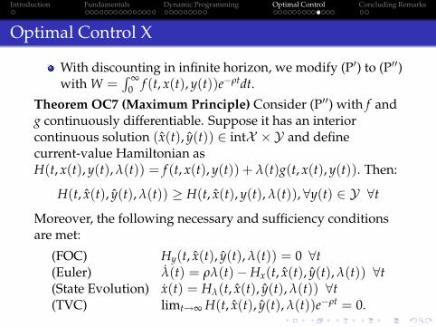
Optimal Control X
With discounting in infinite horizon, we modify (P′) to (P′′)with W =
∫ ∞0 f (t, x(t), y(t))e−ρtdt.
Theorem OC7 (Maximum Principle) Consider (P′′) with f andg continuously differentiable. Suppose it has an interiorcontinuous solution (x(t), y(t)) ∈ intX ×Y and definecurrent-value Hamiltonian asH(t, x(t), y(t), λ(t)) = f (t, x(t), y(t)) + λ(t)g(t, x(t), y(t)). Then:
Introduction Fundamentals Dynamic Programming Optimal Control Concluding Remarks
Optimal Control XI
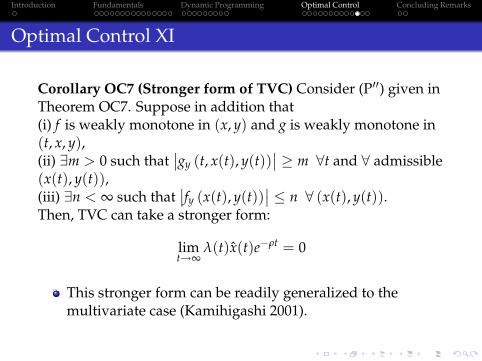
Corollary OC7 (Stronger form of TVC) Consider (P′′) given inTheorem OC7. Suppose in addition that(i) f is weakly monotone in (x, y) and g is weakly monotone in(t, x, y),(ii) ∃m > 0 such that
∣∣gy (t, x(t), y(t))∣∣ ≥ m ∀t and ∀ admissible
(x(t), y(t)),(iii) ∃n < ∞ such that
∣∣fy (x(t), y(t))∣∣ ≤ n ∀ (x(t), y(t)).
Then, TVC can take a stronger form:
limt→∞
λ(t)x(t)e−ρt = 0
This stronger form can be readily generalized to themultivariate case (Kamihigashi 2001).
Introduction Fundamentals Dynamic Programming Optimal Control Concluding Remarks
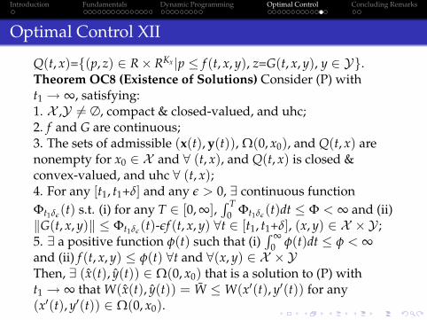
Optimal Control XII
Q(t, x)=(p, z) ∈ R× RKx |p ≤ f (t, x, y), z=G(t, x, y), y ∈ Y.Theorem OC8 (Existence of Solutions) Consider (P) witht1 → ∞, satisfying:1. X ,Y 6= ∅, compact & closed-valued, and uhc;2. f and G are continuous;3. The sets of admissible (x(t), y(t)), Ω(0, x0), and Q(t, x) arenonempty for x0 ∈ X and ∀ (t, x), and Q(t, x) is closed &convex-valued, and uhc ∀ (t, x);4. For any [t1, t1+δ] and any ε > 0, ∃ continuous functionΦt1δε
0 φ(t)dt ≤ φ < ∞and (ii) f (t, x, y) ≤ φ(t) ∀t and ∀(x, y) ∈ X ×YThen, ∃ (x(t), y(t)) ∈ Ω(0, x0) that is a solution to (P) witht1 → ∞ that W(x(t), y(t)) = W ≤ W(x′(t), y′(t)) for any(x′(t), y′(t)) ∈ Ω(0, x0).
Introduction Fundamentals Dynamic Programming Optimal Control Concluding Remarks
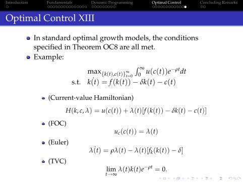
Optimal Control XIII
In standard optimal growth models, the conditionsspecified in Theorem OC8 are all met.Example:
Introduction Fundamentals Dynamic Programming Optimal Control Concluding Remarks
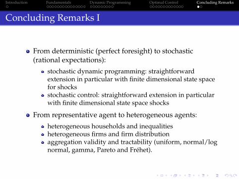
Concluding Remarks I
From deterministic (perfect foresight) to stochastic(rational expectations):
stochastic dynamic programming: straightforwardextension in particular with finite dimensional state spacefor shocksstochastic control: straightforward extension in particularwith finite dimensional state space shocks
From representative agent to heterogeneous agents:
heterogeneous households and inequalitiesheterogeneous firms and firm distributionaggregation validity and tractability (uniform, normal/lognormal, gamma, Pareto and Fréhet).
Introduction Fundamentals Dynamic Programming Optimal Control Concluding Remarks
Concluding Remarks II
From infinite horizon-infinite lifetime to infinitehorizon-finite lifetime overlapping generations (OG):
the prototypical setup is in discrete time (Allais 1947,Samuelson 1958), though there are continuous-time OGwith variational survival (Cass-Yarri 1966, Blanchard 1985)– generalized lifecycle modelswhile the framework is clean, tractable and useful formodeling heterogeneous agents, one must deal carefullywith the following problems:
economy with an infinity of agents (Wilson 1981) and aninfinite of dated goodsgeneric market incompleteness in dated goods trading (noArrow-Debreu securities)generic intergenerational externalities (via preferences ortechnologies)transfer from infinity (Gamow’s Hotel; classic economy;curvature) and lack of market clearing “at infinity” (Cantor)concept of optimality: forward-looking PO andsocial-discounted social welfare maximum.