Page 1
February, 1981
(OSP Number 87272)
FOUNDATIONS OF NONLINEAR NETWORK THEORYPART II: LOSSLESSNESS
J.L. Wyatt, Jr.t, L.O. Chua , J.W. Gannetttt
I.C G tttnar and DN. GreenI.C. Gknar and D.N. Green
Research sponsored by the Office of Naval Research Contract N00014-76-C-0572,the National Science Foundation Grants ENG74-15218 and ECS 8006878, the Inter-
national Business Machines Corporation which supported the third author duringthe 1977-79 academic years with an IBM Fellowship, and the MINNA-JAMES-HEINEMAN-
STIFTUNG, Federal Republic of Germany, under NATO's Senior Scientist Programmewhich supported the fourth author during the 1977-78 academic year.
tDepartment of Electrical Engineering and Computer Science, Room 36-865,
Massachusetts Institute of Technology, Cambridge, MA 02139
ttDepartment of Electrical Engineering and Computer Sciences and the Elec-
tronics Research Laboratory, University of California, Berkeley, CA 94720.
tttBell Laboratories, 600 Mountain Ave., Murray Hill, N.J. 07974.
ttt+Technical University of Istanbul, Turkey.
tttttTRW, Inc., Redondo Beach, California.
Research was partially supported by U.S. Department of Energy under contractET-76-A-01-2295.
� 1�_1�1� 11_11 ______1·_ 1_�____1� � ___�__��_�_ I__�_ ________llllyl__�____ I_.^�
LIDS-P-1068
I
Page 2
4
ABSTRACT
This paper is the second in a two part series [1] which aims to pro-
vide a rigorous foundation in the nonlinear domain for the two energy-based
concepts which are fundamental to network theory: passivity and losslessness.
We hope to clarify the way they enter into both the state-space and the input-
output viewpoints. Our definition of losslessness is inspired by that of
a "conservative system" in classical mechanics, and we use several examples
to compareit with other concepts of losslessness found in the literature.
We show in detail how our definition avoids the anomalies and contradictions
which many current definitions produce. This concept of losslessness has
the desirable property of being preserved under interconnections, and we
extend it to one which is representation independent as well. Applied to
five common classes of n-ports, it allows us to define explicit criteria for
losslessness in terms of the state and output equations. In particular we
give a rigorous justification for the various equivalent criteria in the
linear case. And we give a canonical network realization for a large
class of lossless systems.
-2-
-I -- C I---- -j. ___ ___�'___C-�·I
Page 3
I. Introduction
This paper completes our two-part series [1] on energy-based con-
cepts which are fundamental to nonlinear network theory. Our motivation
for writing this second part is the little recognized fact that lossless-
ness, like passivity, has been given a number of conflicting definitions
[2-4,12,18] in the modern network theory literature. And as before, we
believe that the problem arises from the long period in which "network
theory" meant essentially "linear network theory," since the various
concepts nearly coincide in the linear case.
Unlike its counterpart on passivity [l],this paper differs signifi-
cantly from the theory given in reference [4]. When applied to nonlinear
n-ports, the theory in reference [4] defines losslessness only for pas-
sive n-ports. Other authors [12], [18] would define a lossless n-port
to be a passive In-port which satisfies certain additional conditions.
In this two-part series, we treat passivity and losslessness as indepen-
4ent concepts. As a result of this viewpoint, a more complete theory
emerges. The definition of losslessness given in this paper classifies
a negative linear capacitor as lossless--a very sensible classification--
whereas other approaches are either incapable-of classifying this active
element as lossy or lossless, or they classify it as lossy.
Our definition of losslessness is similar to, but less restrictive
than, the concept of a "conservative system" in classical mechanics [5].
Roughly speaking, we say that a system is lossless if the energy required
to travel between any two points of the state space is independent of
the path taken. This seems to us the most basic doncept possible, and
it is quite different from many definitions found in the literature,
-3-
Page 4
which are based on equations such as
(v(t),i(t)) dt = O (0.)
as in [2], or
'1 tTlim T (v(t),i(t)) dt = 0 (1.2)T+- O
as in [3]. We will show by means of examples that expressions of this
sort must be viewed as criteria for losslessness rather than as defini-
tions of the concept. The relation between the basic definition and
these and other criteria is the subject of Section II.
Notice that the above expressions are purely input-output in charaeL
ter since they involve only the admissible pairs {v(.),i(-)}, whereas
our definition of losslessness relies on a state-space description of the
n-port. This distinction will play a central role in the next two sec-
tions. For example, with losslessness defined as path independence of
the energy, it is clear that an element such as an ideal 1-volt d.c.
voltage source is lossy, at least so long as we view it as a resistive
element. But we could also choose to view it as a nonlinear capacitor
defined by v(q) E 1, and in that case it would of course be lossless.
This raises the disturbing possibility that our concept of losslessness
relies critically on the equations we choose to describe an n-port rather
than reflecting in a straightforward way the physical behavior of the
n-port itself. In fact, we show in Section III that this is not a trivial
anomoly: given any n-port N with a (not necessarily lossless) state
representation S, we can construct a lossless state representation S'
-4-
`1"111111�118�·----··8·- 1-- - - - · _ ,
Page 5
which is equivalent to S. Hence, N always has at least one lossless
state representation. If we say, "a lossless n-port is an n-port with
a lossless state representation," then every n-port is lossless and the
definition means nothing at all. In Section III we show that if there
exists a lossless state representation for N which satisfies a certain
observability requirement, then (essentially) all state representations
for N are lossless. This result allows us to formulate a meaningful
definition of losslessness for an n-port, and it completely resolves the
anomoly described above.
In Section IV we show that the internal energy functional] for a
passive n-port becomes unique in the lossless case. Aid in Section V
we derive explicit criteria for losslessness in terms of the state and
output equations of several special classes of n-ports. In particular
we show that the criteria (1.1) and (1.2) are equivalent to losslessness
in the linear, time-invariant, finite dimensional case, which explains
why they are often invoked as definitions. And Section VI is devoted
to a canonical network realization of lossless n-ports which becomes
possible under certain assumptions.
In this paper, n-ports will be mathematically modeled by state repre-
sentations (a complete list of our technical assumptions and definitions
is given in Section II of [1]). Briefly, a state representation is a
set of state, output, voltage, and current equations
x(t) = f(x(t),u(t)) (1.3)
y(t) = g(x(t),u(t)) (1.4)
v(t) = V(x(t),u(t)) (1.5a)
-5-
11�1__� 11�_______�1� 1��__ �_ �____�L1_·l__ �__�___ _�____·I__ �_____�
Page 6
i(t) = I(x(t),u(t ) ) (1.5b)
where f(.,.), g(.,.), V(.,.), and I(.,.) are all continuous functions
defined on x U C Rm xRn (Z - state space, U set of admissible input
values). The inputs u(-) belong to a set U of functions mapping R =
[O,o) to U. For each input u(-) and each initial state x(O), we assume
the existence and uniqueness of the solution to (1.3) over the time
interval R+. The power input function is defined by (x,u) A (V(x,u),
I(x,u)) , we assume that t + p(x(t),u(t)) is locally L1 for every input-
trajectory pair. The energy consumed by an input-trajectory pair
{u(.),x(.)}J[O,T] is the quantity f p(x(t),u(t))dt--note that this
quantity can be positive, negative, or zero.
We will continue to make the blanket assumption that U is translati6i
invariant and closed under concatenation [1, defs. 6 and 7]; but uikd
[1], we will no longer repeat these assumptions explicitly when a theorem
or lemma requires them.
II. Five N-Port Attributes Associated with Losslessness
Five characteristics of an n-port which are. frequently associated
with losslessness are, in rough order from the most obvious to the most
subtle:
1. zero energy required to drive the state around any closed path,
2. the existence of a scalar function of the state which "tracks"
the energy entering the ports,
3. all the energy which enters the ports can be recovered at the
ports,
4. the total energy entering the ports over the time interval [0,co
-6-
�-"--"-�-� ------ -- --- I- - - --- - - I - -·r`i--·---
Page 7
is always zero, and,
5. the average power entering the ports over the time inverval
[O,T] is always zero in the limit as T + ~.
Note that properties 1 and 2 involve state-space ideas, while 3-5
are purely input-output in character. Although properties 1, 2 4, and
5 have all been used by various authors to define losslessness, only
property 3 means literally "no loss of energy."
We will give a detailed discussion of these properties in subsec-I
tions 2.1 through 2.5, and we will mention here only the major conclu-
sions. It might appear on first reading that these five concepts and
losslessness itself are simply different ways of saying the same thing.
But it is rare in systems theory for input-output and state-space con-
cepts to coincide exactly without restrictive assumptions, and this case
is no exception. The major conclusion which emerges from this section
(indeed, our motivation for writing it) is that not one of these five
notions is known to be strictly equivalent to losslessness, defined as
path-independence of the energy. The first two will turn out equivalent
to losslessness under the additional assumption f complete controllability
[1, def. 13], but the last three will not be unless very restrictive
assumptions are imposed.
Relationships weaker than equivalence certainly do exist, though.
It is not hard to see, for example, that losslessness and complete controlla-
bility imply property 3. And we will present a more stringent set of
assumptions under which property 5 implies losslessness.
The following definition is a rigorous statement of the concept
of losslessness as path independence.
-7-
__ �_�____��_ -- _-�11�_·_�1__
Page 8
Definition 2.1. A state representation S is defined to be lossless if
the following condition1 holds for every pair of states xa, xb in . For
any two input-trajectory pairs {u (.),) } l[O,Tl],{u2 (-) ,x 2(. )} [O ,T2 ]
from x a to xb, the energy consumed [1, def.8 ] by {Ul(-),xl( )}l[O,T1]
equals the energy consumed by {u2(.),x 2(-)l}[0,T 21. A state representa-
tion which is not lossless is defined to be lossy.
Note that Definition 2.1 does not require that there exist two or
more input-trajectory pairs between every pair of states xa and Xb:
there may exist only one input-trajectory pair between xa and Xb, or none
at all. Also, a state representation which has no more than one input-
trajectory pair between every pair of states is lossless by default.
As we discussed inthe introduction, this notion of losslessness is
dependent upon the particular state representation we choose for an
n-port. For this reason we will initially consider losslessness to be
an attribute of a state representation S rather than of an n-port N.
We will show later, in subsection 3.1, that we can rid ourselves of this
dependence on S under certain reasonable assumptions and define lossless-
ness directly as an attribute of N. In the next two subsections we will
discuss the concepts of cyclo-losslessness and conservative potential
energy functions, which suffer from this same dependence on S. In sub-
section 3.2 we will give conditions under which they can be made repre-
sentation independent as well.
1Since U is translation invariant [1, Def. 6] and the state equations are
independent of time, there is no loss of generality in assuming that bothtrajectories pass through a at t = 0. 'And because of our standingassumption [1, Section II] that t -+ p(x(t),u(t)) is locally L1 , theenergy consumed over any finite time interval is always finite.
-8-
�_�_1��1� 1 __ _____ i
Page 9
2.1. Cyclo-Losslessness
We will say that a state representation is cyclo-lossless if the
energy required to drive the system around any closed path in its state-
space is zero. The following definition says this a bit more formally.
Definition 2.2. A state representation S is defined to be cyclo-lossless
if for every input-trajectory pair {u(-),x(-)} and every T > 0 such that
x(O) = x(T), the energy consumed by {u(),x(-)}[[OT] is zero.
This is essentially the definition of a conservative system in
classical mechanics [5], and it is slightly less restrictive than the
definition of cyclo-losslessness given by Hill and Moylan [18].
Like losslessness itself, cyclo-losslessness is not a pure input-
output concept but depends upon the particular state representation we
.choose. The ideal voltage source, for example, is cyclo-lossless when
considered as a capacitor but not when considered as a resistor. To see
that losslessness and cyclo-losslessness are not entirely equivalent
concepts, consider the following example.
Example 2.1. If the current-controlled 2-port in Fig. 1 is given the
obvious state representation in terms of ql and q2, it will be lossy
because of the resistor. But it is cyclo-lossless "by default," because
(ql(0),q 2(0)) = (ql(T),q2(T)) is possible only if we don't excite port
#l over the interval [O0,T].
Nonetheless, there is a very strong relationship between the two
concepts as the following lemma shows.
Lemma 2.1. Let S denote a state representation. Then the following
three statements are true:
-9-
_I __1�1 · _�___ ____ __I_^____�_�__________�___ _
Page 10
a) If S is lossless, then S is cyclo-lossless.
b) If S is completely controllable and if there exists a state
0 E for which every input-trajectory pair {u(-),x()}[ O,T] with
x(O) = x(T) = O consumes zero energy, then S is lossless.
c) If S is cyclo-lossless and completely controllable, then S is
lossless.
Lemma 2.1 is fairly obvious, but a rigorous formal proof is given in
Appendix A. In essence, the lemma says that losslessness and cyclo-
losslessness are equivalent concepts for completely controllable systems.
Statement b) of the lemma will be utilized in our proof of results for
linear systems.
2.2. Conservative Potential Energy Functions
A conservative potential energy function is a scalar function defined
on the state space, which increases along trajectories at the same rate
that energy enters the ports. The following definition just says the
same thing more precisely.
Definition 2.3. A function : + IR is defined to be a conservative
potential energy function for a state representation S if
t 2
(t 2 )) - L(tl)) = J p(x(t),u(t))dt (2.1)t1
for all input-trajectory pairs {u('),x(.)} and all 0 < t < t2 < .
It is evident that every state representation with a conservative
potential energy function is lossless, and that any two conservative
potential energy functions for a given state representation can differ
only by an additive constant on any region of reachable from a given
point x E . Note that any nonnegative conservative potential energy
-10-
------ '-- " I �`----�I�-���--�-'I�-~--------�`--`"I
Page 11
function is also an internal energy function [1, Def. 23].
Like losslessness and cyclo-losslessness, the concept of a con-
servative potential energy function is not purely input-output in
character, but involves the state space in a fundamental way. The ideal
1-volt d.c. voltage source, for example, has the conservative potential
energy function (q) = q if we view it as a capacitor; but there is no
conservative potential energy function for this system if we view it as
a resistor.
In this section we will be content to define conservative potential
energy functions in terms of a given state representation S. In subsection
3.2 we will discuss the conditions under which a conservative potential
energy function can be assigned to an n-port N, independent of our choice
for S.
The following simple lemma shows that under a certain reachability
assumption, every lossless state representation has a conservative
potential energy function. We do not know whether this conclusion holds
W;thout such an assumption.
Lemma 2.2. 'Suppose a state representation S is lossless and that there
exists some state x E Z such that all of is reachable 1, Def. 12] from
x. And let (x) represent the energy required to drive the state from
x to any point x E S. Then :E + IR is a conservative potential energy
function for this state representation.
The proof is in Appendix A. Since the reachability assumption in
Lemma 2.2 is always satisfied by completely controllable systems, it
follows that losslessness, cyclo-losslessness, and the existence of a
conservative potential energy function are all equivalent concepts for
completely controllable state representations.
-11-
II- - I_-----�-----I�_-_-
Page 12
We haven't required or assumed that a conservative potential energy
function be continuous, much less differentiable. But in those cases
where is continuously differentiable, it is possible to rephrase (2.1)
in differential form as follows.
Lemma 2.3. Let S denote a state representation, and suppose that is an
open subset of IRm . Suppose further that U satisfies the following mild
technical assumption: for each u0 E U, there exists an input u(.) E U
such that u(O) = u0 and u(.) is continuous at t 0. Then a C1 function
: 7 + IR is a conservative potential energy function for S v
(Vq(x),f(xu) = p(x,u) (2.1a)
for all (x,u) E x U.
The proof is in Appendix A.
Note carefully that a conservative potential function need not be
differentiable at all. It is an open. question whether * will be dif-
ferentiable even when f(,*) and p(,-) are C . (We have discussed a
related question at length in [1, example 7].) Therefore the existence
of a function satisfying (2.1a) is not known to be anecessary condition
for losslessness, even for completely controllable systems where f(., )
and p(-,.) are C
2.3. Energetically Reversible Systems
A third property associated with losslessness is the property of
being an "ideal energy reservoir," i.e. that all energy pumped into the
system through its ports can be recovered at a later time. This is a
genuine input-output property; therefore, if a state representation for
an n-port N has this property then all state representations for N will
have this property.
__lii_111_1______13I__IIIIL_____C ----- - -- , �I� ,_ ---�.I ----i-- �
Page 13
Definition 2.4. A state representation S is defined to be energetically
reversible if the following condition holds for each x E . For every
admissible pair (v(.),i(.)} with initial state x and every T > 0, there
exists an admissible pair {v'(.),i'(-)} with the same initial state x,
and a T' > T, such that
i) {v(t),i(t)} {v'(t),i'(t)}, Vt E [,T]
ii) (v' (t),i'(t))dt = 0. (2.2)
An n-port is defined to be energetically reversible if it has an
energetically reversible state representation.
Condition i) and the requirement that {y(),i()} and {v'(-),i'(.)}
have the same initial state imply that {y'(-),i'()}(T,) is a develop-
ment of the port voltages and currents in time which remains possible
for N at the moment T, after the waveforms {v(.),i(.)}j[0,T] have been
observed. In the light of this observation, (2.2) means that all the
energy deposited in N over the interval [0,T] can be recovered over some
interval (T,T'].
An n-port is energetically reversible if, from the viewpoint of the
outside world, no energy can ever disappear or be lost inside it. For
this reason we were once tempted to adopt Def. 2.4 as our definition of
losslessness. But we have decided to define losslessness as path
independence of the energy instead, since the latter concept corresponds
more closely to the standard electrical engineering usage of the term.
While it may seem natural to associate energetic reversibility with
losslessness, the former property is neither a necessary nor a sufficient
condition for the latter. For example, a 2-terminal resistor whose
constitutive relation (v-i curve) contains points in both the first and
second quadrants is a lossy element which is energetically reversible.
-13-
Page 14
And the -port in the following example is lossless but tot energetically
reversible.
Example 2.2. The 1-port in Fig. 2 has the following state representation:
4 = 12 (i+jil)
if i > O,
Ti, if i < 0.
This -port is clearly lossless, but it is not energetically reversible
because of the ideal diode in series with the capacitor. (Note that this
example violates our technical assumptions because the port voltage is
not a continuous function of q and i. This violation does not arise if
one makes the artificial (but permissible) restriction i > O.)
In spite of Example 2.2, there is a strong connection between the
state dependent property of losslessness and the input-output property
of energetic reversibility, as the following'lemma shows.
Lemma 2.4. Suppose that a state representation S is lossless and
completely controllable. Then it is energetically reversible.
The proof is in Appendix A.
2.4. The Zero Total Energy Property
The zero total energy property is the term we have adopted to
express conditions of the type
p(x(t),u(t)dt = 0 (2.3)
where appropriate restrictions may be placed on the input-trajectory
pairs {u('),x(.)} for which (2.3) is required to hold. The zero energy
-14-.
- -- "-� -- - --- ---- --- _ �
Page 15
idea is rather appealing in the usual case that u(') and y(-) are a
hybrid pair [1, Def. 3. For then (2.3) becomes
J (u(t),y(t))dt = 0 (2.4)
and has the straightforward geometric interpretation that u(') and y(.)
are orthogonal in the Hilbert space L2(R+ +IRn). In other words, if U
and V are contained in L2, then (2.4) says that the n-port acts as an
operator which maps each input waveform u(-) into the subspace of L
orthogonal to u(-). In this guise the zero total energy property appears
as a generalization to function spaces of the idea of a nonenergic
n-port [6], one for which v(t) and i(t) are orthogonal vectors in IR
at each instant t.
There are many possible versions of the zero total energy property,
depending upon the conditions we place on u(-) and x(-) or u(·) and
y(-). Since no single version is really definitive for our purposes,
we will describe some of the most significant variations and their
relation to losslessness.
A version of the zero tptal energy property was proposed in [2] as
the definition of losslessness in both the linear and the nonlinear case.
In the language of this paper, the definition in [2] can be paraphrased
as follows. "An n-port N is lossless if
f(v(t),i(t))dt = 0 (2.5)
holds for all admissible pairs {v( ),i(-)} in L2(R+ >R n) so long as
there is no energy stored in N at T = O." This conception of losslessness
is adequate as a criterion in the linear theory, but the following
example shows that it is inappropriate for nonlinear systems.
-15-
------ �1111 -- _1..� 1_��_111�_1 _ _
Page 16
Example 2.3. Consider the 1-port capacitor with the constitutive relation
f q, q< O
v(q) = sin q, 0 < q < f
0 , q> r
shown in Fig. 3a. If we give it the usual state representation for a
capacitor, with q as the state variable, then it is clearly lossless
(Def. 2.1). In fact, it has properties 1), 2), and 3) listed at the beginning
of this section, and property 5 holds also if {v(),i(-)} is bounded. But to
see that it doesn't satisfy the definition in [2], consider the following signal
pair, shown in Fig. 3b:
1, 0 < t < in(t) 0 < t < i(t) = <---- v(t) =
0, otherwise , otherwise.
This is an admissible pair if the initial state is q(O) = 0, and it is
clearly in L . The "stored energy" is initially zero in this case, but
the total energy entering the ports is 2 joules. Thus the definition in
[2] would have to classify this capacitor as lossy, which is contrary
to the intuitive view that a l-port charge-controlled capacitor with
a continuous constitutive relation ought to be lossless.
Nonetheless, the following two lemmas show that there is a definite
relation between losslessness, as we define it, and certain versions of
the zero total energy property.
Lemma 2.5. Suppose a state representation S is lossless and completely
controllable. Then S has a conservative potential energy function 4,
and we suppose further that is continuous. Under these conditions,
lim f (v(t),i(t))dt = 0 (2.6)T4- 0
'416,
I� _r � � _ X
Page 17
for all (not necessarily L2) admissible pairs {v() = V((.),u()) ,i()
I((x('),u(')) } such that lim x(t) = x(O). Furthermore, (2.5) holds
2 t-ofor all L admissible pairs such that lim x(t) = x(O).
The proof is in Appendix A. The difference between equations (2.5)
and (2.6) is a technical point based on the definition of the Lebesgue
integral [7]. Because of our standing assumption that t + (v(t),i(t))
is locally L1, the integral in (2.6) will necessarily exist for each
finite value of T. But the integral in (2.5) exists only if the positive
and negative parts of (y(.),i(-)) individually yield finite values when
+integrated over all of JR , a mathematically stronger assumption which
explains our requirement that in that case v(-), i(-) E L (R +lR ).
Lemma 2.6. Suppose that a state representation S is lossless. Then
- T
f p(x(t),u(t))dt = 0
for all input-trajectory pairs {u(-),x(.)} such that x(-) is a periodic
function with period T, and for each integer n > 0.
Lemma 2.6 follows immediately from statement a) of Lemma 2.1.
Note that the versions of the zero total energy property invoked
in these two particular lemmas are not purely input-output in character
since they include restrictions on the state-space trajectory x().
2.5. The Zero Average Power Property
Definition 2.5. A state representation is defined to have the zero
average power property if
lim. (v(t),i(t))dt = 0 (2.7)T-+ 0
-17-
�-� �-`��--�-� �1------�--- --� �- ---- �--"- I I-"------------------- --
Page 18
for every admissible pair {v(),{(.)} such that v(.) and i() are
bounded functions. An n-port is defined to have the zero average power
property if it has a state representation with the zero average power
property.
Since Definition 2.5 involves only the admissible pairs of a'system,
it is purely input-output in character. Therefore if an n-port N has the
zero average power property, then all state representations for N have
the zero average power property.
This property and variations on it have been commonly associated with
losslessness in the literature on linear network theory. It has even
been proposed as a definition of losslessness for nonlinear algebraic
n-ports [3]. But we shall present examples, admittedly somewhat contrived,
which show that the zero average power property is neither a necessary
nor a sufficient condition for losslessness in general.
Our stipulation that (2.7) need only hold when v(-) and i(.) are
bounded requires some explanation. In keeping with the traditions of
linear circuit theory, we would certainly want to say that a 1-farad
capacitor, for example, has the zero average power property. But (2.7)
doesn't hold for all admissible pairs of a 1-farad capacitor, as we can
see by considering the admissible pair {i(t) = 1, v(t) = t}. We could
eliminate this particular admissible pair from consideration by requiring
that v(.), or the state-space trajectory x(-) = q(-), or both be bounded.
It turns out that a sensible general theory emerges only if we require
boundedness of v() and i() but not of x(.). A detailed discussion of
this point is given in Appendix B.
Exple 2.4.
To produce a voltage-controlled state representation for the 1-port
in Fig. 4, we define f by
-18-
Page 19
v-vc v > vf(v,) =c
c e , V < .
Then f is continuous, and the voltage-controlled state equations are
Vc = f(v ,v), i = f(vc,v). Since we are only interested in bJ inded
admissible pairs, we can take U = L (IR -R).. It is easy to see that
this is a lossy state representation.
To show that Example 2.4 has the zero average power property, let
{v(.),i(-)} be any bounded admissible pair. Then there exists a finite
constant M > 0 such that v(t)J < M and i(t)I < M for all t. Since
f(vc,v) > 0 always, it follows that i(t) > 0 for all t and v C.) is
monotonically increasing. If vc(t) = Vc(0) for all t, then i(t) = 0 for
a.a.t E R+ and (2.7) is trivially satisfied. Now suppose that Vc() is
not constant. Then it is obvious from the circuit shown in Fig. 4 that
v¢(t) < M for all t E R + . To prove this assertion rigorously, suppose
1
that vC(t ) > M for some t o E IR- . Define a.A sup{t > t: v(t) > M}.
4y the continuity of vc(.), a > t; and by the definition of a, vc(t) > M
for all t E [to,a). But whenever vc(t) > M, it.must be constant (because
f(v (t),v,v()) = 0; i.e., no current can flow through the ideal diode).
Thus vc( ) is constant on the interval [to,a). If a < , then, by
continuity, Vc(a) = lim vc(t) = vc(t0) > M, and so there exists an > 0
·t<asuch that Vc (a+c) > M, which contradicts the definition of a. Therefore
vc(') is constant on the interval [to,), and a similar argument shows
that vc() is constant on the interval [O,t0]. These facts contradict
the assumption that vc(.) is not constant; hence, v(t) < M for all t.
Now
-19-
_ �_
Page 20
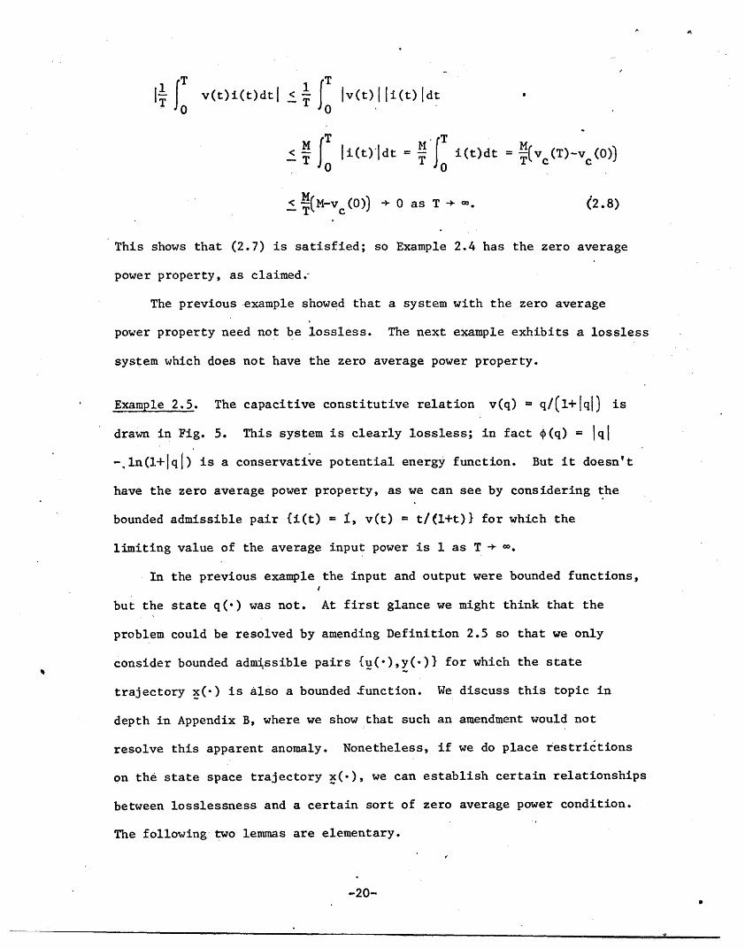
M | VI(t) dt| T Iv(t) I i(t) dtT T v(t)i(t)dtl II 0
0 0
M Ii(t) T | i(t)dt = (vc (T)-v c(O ))li(t)Ildt M 0
M(M-vc( 0) ) + 0 as T + . (2.8)
This shows that (2.7) is satisfied; so Example 2.4 has the zero average
power property, as claimed.-
The previous example showed that a system with the zero average
power property need not be lossless. The next example exhibits a lossless
system which does not have the zero average power property.
Example 2.5. The capacitive constitutive relation v(q) = q/(l+Iql) is
drawn in Fig. 5. This system is clearly lossless; in fact (q) = q
-ln(l+lql) is a conservative potential energy function. But it doesn't
have the zero average power property, as we can see by considering the
bounded admissible pair {i(t) = , v(t) = t/(l+t)} for which the
limiting value of the average input power is 1 as T + a.
In the previous example the input and output were bounded functions,
but the state q(') was not. At first glance we might think that the
problem could be resolved by amending Definition 2.5 so that we only
consider bounded admissible pairs {u('),y(-)} for which the state
trajectory x() is also a bounded Function. We discuss this topic in
depth in Appendix B, where we show that such an amendment would not
resolve this apparent anomaly. Nonetheless, if we do place restrictions
on the state space trajectory x(), we can establish certain relationships
between losslessness and a certain sort of zero average power condition.
The following two lemmas are elementary.
-20-
-- .�-- �----- �-�� -·---·-·-------�.���---� ..�-.--·-��.1���-` .- ��- ·1
9.
Page 21
Lemma 2.7. Suppose the state representation S is lossless and completely
controllable, and that its state space is all of R . Then S has a
conservative potential energy function , and we suppose further that
4 is continuous. Under these conditions, (2.7) holds for all admissible
pairs {v(.),i(.)} = {V(x()),()) x(-),u())} such that xfo) is bounded.
The proof is given in Appendix A.
Lemma 2.8. If a state representation S is lossless, then (2.7) holds
for all admissible pairs fv( ),i((.)} -, such
that x() is a periodic function.
The proof is given in Appendix A.
These two lemmas do not yet show a relationship between losslessness
and the zero average power property as in Definition 2.5, because they
require additional information about the state trajectory x(). Can we
find a connection between losslessness and the purely input-output
statement of the zero average power property, one which holds for non-
linear n-ports and nonperiodic inputs and trajectories? Examples 2.4
and 2.5 place rather restrictive bounds on possible theorems in this
area, but Lemma 2.8 suggests that we might have some success if we could
find a way to reduce the general case to the periodic case. In linear
circuit theory the Fourier transform does exactly that, but we must
find another approach for nonlinear systems. First, we need the following
technical definition, the terms of which are illustrated in Fig. 6.
Definition 2.6. Given u(.) :IR+ - R n, we let u(.)l[O,T) denote the
restriction of u(.) to the interval [O,T), T > 0. Given u(-) and T > 0
+ nwe say that w() R + IRn is the periodic extension of u(-)l[0,T) if
for each .t E R , w(t) (t-nT), where n is that unique nonnegative
integer such that t-nT e [0,T). (See Fig. 6.) Finally, we say that U
-21-
_
Page 22
is closed under periodic extension if for each u() C U and each T > 0,
the periodic extension of u(.)j[O,T) is also an element of U.
Although "closure under periodic extension" bears a superficial
Resemblance to "closure under concatenation" [1,Def.7], it is actually a
quite different concept. The essential difference is that closure under con-
catenation means one can piece together two (and hence any finite number)
of different waveforms, whereas closure under periodic extension means
one can piece together a segment of any single waveform an infinite number
of times with itself. Consider Fig. 6 again. The waveform u() in
Fig. 6a belongs to all the spaces LP(R +IR), 1 < p < a, since it is
bounded and vanishes outside some finite interval. On. the other hand
the periodic extension of u(.)j[O,T), shown in Fig. 6c, is in L but not
in Lr, 1 < r < . Thus while all the LP spaces are closed under con-
catenation, only L is closed under periodic extension.
The following theorem gives the relation between the input-output
property of zero average power and the state-space property of losslessness.
Theorem 2.1. We are given an n-port N with state representation S
satisfying the following assumptions:
i) S is completely controllable,
ii) U is closed under periodic extension,
iii) each waveform in U is bounded on every compact interval [O,T],
and
iv) V(-,.) and I(-,-) are bounded on every bounded subset of x U.
Under these conditions, if S has the zero average power property then S
is lossless.
Remark. Assumptions iii) and iv) are rather technical and not very
restrictive. For example if U contains only piecewise-continuous waveforms
-22-
_ ___�_ __���_ ______I_______/_____bsll__�l_____l_ � �_�_ _.__I I
Page 23
then iii) is satisfied automatically, and if = IRm and U n then
iv) is satisfied automatically because we have assumed that V(,.) and
I(.,-) are continuous [1, section II]. Assumptions i) and ii), on the
other hand, are essential. The theorem fails without assumption i), as
we see from Example 2.4, Fig. 4. It also fails without assumption ii),
for consider the (admittedly artificial) example of a 1 ohm resistor
2 +with u = i where we make the very special choice U L (R 1R). This is
a lossy system, ut it has the zero average power property as a result
of U being L2 , a space which is not closed under periodic extension.
Proof of Theorem 2.1. The proof proceeds by contradiction. We will
assume the system has the zero average power property and satisfies
assumptions i)-iv) but is lossy. A contradiction will emerge.
If it is lossy, then there exist two states x , xb in Z and two
input-trajectory pairs {u1( ),x 1(.)}[O,T1], {u2 (.),x 2()}1[ 0,T2] from
Xa to Xb such that E1l E2, where E1 is the energy consumed by
{Ul(-),Xl(.)}I[O,T1] and E2 is the energy consumed by {u2 ('),x 2 ([)}[0,T 2 ]
[1, Def. 8]. (See Fig. 7.)
Since the system is completely controllable, there is an input-
trajectory pair {u3(-),x 3 ()}1I[0,T 3] from xb to X , and we let E3 be-3 -3 3 _b -a3
the energy consumed by {u3(.),x 3(-)}f[0,T3]. And since E1 E2, either
EI+E 3 0, or E2+E 3 0, or both. For definiteness, suppose E+E 3 O0.
Let u4 () consist of u1 (-) followed by u3 (-), i.e.
u(t) = 0l(t), < t< T
U3(t-T1)' t > T1
Since U is closed under concatenation, u4 ( ) E U. And since the state
equations are time-invariant, {u4(.),X 4(-)1 is an input-trajectory pair,
where
-23-
I �I�___ _ ��____1_______1__1_1�_� 1--
Page 24
x4(t) - (t) Ot<Tl, 0 < t < T3(t-T1), t > T1
(Note that x(T) = x3 (0)). Then x4(T1) = xb and x4() = (T+T 3) = xa,
so x4 () passes once around a loop. And the energy consumed by
{U4(. X4( )}I[0,T+T3] is E+E 3 O0.
To complete the construction of a contradiction,we just drive x around
the loop forever. More formally, let a4 (-) be the periodic extension of
U4(.)I[0,T1+T3). Since U is closed under periodic extension, 4(-) E U.
And since the state equations are time invariant, {4 (),x 4(*)} is a valid
input-trajectory pair if X4(.) is the periodic extension of x4 (.)![0,Ti+T3).
This furnishes our contradiction, since
n(T+T 3) n(1+E 3)
n (TT ) 0 p(x4 (t), 4(t))dt = n(T+T 3)
E1+E3
T1+T 3
for every positive integer n. In order to prove that (2.9) genuinely
contradicts our assumption that the system has the zero average power
property, as in Def. 2.5, we must verify that V(x4( ),u4( )) and
It(),u4() ~are bounded. Since X4 (*) is continuous and periodic it
is bounded. And U4(.) is bounded by assumption iii), since it is also
periodic. Therefore V(x4( ),u4( )) and I(x4( ),u4 ( )) are bounded by
assumption iv). n
Corollary. If a system satisfies the assumptions of Theorem 2.1 and
has the zero average power property, then it is energetically reversible.
This follows from Theorem 2.1 and the fact that a lossless, completely
controllable state representation is energetically reversible (Lemma 2.4).
-24-
_ _I__ _ _ __ _1 __~~~~~~~~~~~1____1___1_11_______~~~~~~~~~~~ -·-·- _.l__·_-·C-·~~~~~~~~~~~-~~~_l~~_ I____ _~~~~~ __.____ __~~~~~
Page 25
III. Representation Independence and Closure
In subsection 3.1 we define the term "total observability" for
state representations, a concept which is essentially the same as the
usual "complete observability" in system theory. Our main result is
to prove that losslessness is a genuine physical property of anr n-port,
independent of the particular state representation we choose for it, so
long as we restrict ourselves to totally observable state representations.
In subsection 3.? we give related results for cyclo-losslessness and
conservative potential energy functions. And in subsection 3.3 we will
make precise the idea that an interconnection of lossless n-ports is
itself lossless.
3.1. Losslessness, Total Observability, and Equivalent State
Representations
The example of a d.c. voltage source, which is lossless when viewed
as a capacitor but lossy when viewed as a resistor, raises a serious
question about the physical significance of our definition of losslessness.
Is losslessness a genuine physical property of an n-port, or is it merely
an artifact of the particular state representation we choose for it? The
following example shows how pervasive an issue this is.
Example 3.1. Given any n-port N with a state representation S consisting
of the equations x = f(x,u), y = g(x,u) and some specification for U, U
and , it is possible to create a lossless state representation S' for N
as follows. We augment the state space by one dimension, defining
Z' _ x R, and then we add an artificial state variable e(t) which
measures the total energy which has entered the ports over the interval
[O,T]. The state of the new system is (x,e), and its equations are
-25-
I__lll___a_____L�I_________l��___l__ _
Page 26
(: G p(x,u)
y g(X,).
The new state representation S' is obviously lossless because the
energy required to travel between two states is now just the difference
in their last coordinate. But S' is definitely peculiar because the
artificial state variable e is not directly represented in the output
y, which depends on x and it alone. The state representation of a d.c.
voltage source as a capacitor has this same peculiarity-- its "charge"
doesn't affect its output. By weeding out these "unobservable" state
representations, we will be able to attach a definite physical meaning
to losslessness after all.
Definition 3.1. Let S and S be two (not necessarily distinct) state
representations. State x of S and state x of S are defined to be
equivalent if the set of admissible pairs of S with initial state x is
identical to the set of admissible pairs of S with initial state x.
S is defined to be state-observable if the equivalence of any two states
x1 and x2 of S implies that x1 = x2.
In other words, S is state-observable if and only if the following
condition is satisfied: if xl Z x2, then xl and x2 are not equivalent.
State-observability as defined above is essentially the standard notion
of (complete) observability from system theory [11], the only difference
being that it is stated in terms of admissible pairs, rather than input-
output pairs. We have given it the name "state-observability" in order
to distinguish it from the concept of "inp.ut-observability," which will
be defined shortly. First, however, some discussion on equivalent state
-26-
- �--�X------r�-� --� -------- - -------------·----·-- ---
i
Page 27
a
representations is in order.
Definition 3.2. Two state representations, S and S , are defined to be
equivalent if for any state x of S there exists an equivalent state x.
of S , and conversely, for any state x of S there exists an equivalent
state x of S.
This is essentially the definition of equivalence given by Desoer
[11]. Definition 3.2 is less restrictive than the definition of equi-
valence.given in Part I of this series [1, Def. 19, p. 29]. The reasonI
we are changing our definition of equivalence is to clear up a vague
point in Part I. We consider two state representations to be (equally
valid) mathematical models for the same n-port if and only if they are
equivalent according to Def. 3.2: this is implicit from the discussion
throughout this paper and its counterpart on passivity. An illustration
is afforded by our recurrent example of a 1-volt d.c. source, which has
both resistive and capacitive state representations. Definition 3.2
properly classifies these state representations as equivalent, whereas
Definition 19 in [1] does not. The same comment applies to the two state
representations S and S' in Example 3.1.
Another vague point in Part I was that we never explicitly stated
how we view an n-port within the framework of our theory. This situation
is rectified by the following statement: An n-port is identified with an
equivalence class [7] of state representations, where the equivalence
relation is given by Definition 3.2. When we say that an n-port N "has"
a state representation S (or that S is a state representation "for" N),
we mean that S is an element of the equivalence class which is identified
with N.
When we say that a property is representation independent, we mean
that if a state representation S has that property, then all state
-27-
�I�
Page 28
representations equivalent to S have that property also. It is easy to
see that the theorem for representation independence of passivity
[1, Theorem 8] remains valid with the less restrictive form of equi-
valence given in Definition 3.2. In Part I we defined an n-port to be
passive if it has a passive state representation; thus, by representation
independence, all state representations for a passive n-port are passive.
Although a new form of equivalence has been introduced in Definition
3.2, the concept'of equivalence given in Part I [1, Def. 19] will continue
to be of interest to us. In order to avoid confusion, we shall henceforth
refer to it as "bijective equivalence." Formally, ,we have the following
definition.
Definition 3.3. Two state representations, S1 and S2, are defined to be
bijectively equivalent if there exists a bijective map b Z: + - such that
for each x E E1, the class of admissible pairs of S1 with initial state x
is identical to the class of admissible pairs of S2 with initial state
b(x).
Lemma 3.1. Suppose S1 and S2 are bijectively equivalent state
representations. Then S1 is state-observable S2 is state-observable.
The proof is given in Appendix A.
Definition 3.4. A state representation S is input-observable if the
following condition holds for any two input-trajectory pairs
(U l(),Xl()}, {u2(w)x2()} with a common initial state xl(O)- x2(0).
If ul(t') u2 (t') at some time t' > 0, then {(l(t),ul(t)), I(xl(t),ul(t)) }
{ y{(X2(t),2 (t))x2(t),u2(t))} for some t [0, t'].
Input observability means that to any admissible pair v(-),i(')}
with a given initial state x0, there corresponds exactly one input
-28-
�--l�i-�11 I(l�-------L-·---··-·---··-)·1�-··�···I�
Page 29
waveform u(-). In conjunction with our assumption that solutions are
unique, it implies that to any admissible pair {v(-),i(.)} with given
initial state x0 there corresponds a unique input-trajectory pair
{u(-),x(-)}. We have defined this concept only in order to state our
lemmas and theorems in a rigorously correct way; it is always satisfied
in any practical case. For example, all hybrid and transmission
representations are automatically input-observable because the inputs are
a subset of the port voltages and currents. In these gases, the inequality
in Definition 3.4 will be satisfied at t t'.
If we make the modest technical assumption that for each ug E U there
exists a u(.) E U such that u(O) = u, then input obsertability implies
that the mapping u + {V(x,u),I(x,u)} from U to IRn x IRn is injective for
each fixed x E . We do not know whether this condition is sufficient
for: input observability.
Definition 3.5. A state representation is defined to be totally
observable if it is both state-observable and input-observable.
Before proceeding to the next lemma, a few technical comments are
in order. Let S1 and S2 be two equivalent state representations, and
suppose that S2 is state-observable. Then, by the definition of
equivalence, for each state of S1 there exists a state 2 of S2 which
is equivalent to S1; moreover, because S2 is state-observable, x2 is
unique. Thus there exists a unique map a Z1 + Z2 such that for each
state x1 of S1, ((xl) is the unique state of S2 which is equivalent to
x1. If, in addition, S1 and S2 are input-observable, then the map a(-)
"matches up" the entire state trajectories of those input-trajectory
pairs which produce identical port voltage and current waveforms in the
two systems. This is stated precisely in the following lemma.
-29-
I --C --�- ·-�-�I*�---·�·II-·�-3·* -�--I--
Page 30
4
Lenma 3.2. Let S and S be equivalent state representations, with S11 21
input-observable and S2 totally observable. Let : C 1 + E2 denote the
unique map such that for each state x of S1, a(x) is the (necessarily
unique) state of S2 which is equivalent to x. Let T > 0 be any time and
let {ul(),l(-)}I[0,T] and {u2(.)x2 (.)}j[0,T] be any input-trajectory
pairs of S1 and S2, respectively, such that {Vl(x l(t),u l (t)),
Ii(xl(t)ul(t))} = {V2(x2(t),u 2(t)),I2(X2(t),u2(t))} for all t E [O,T],
where V1(;,-), I(.,.) are the readout maps for S1, and V2( -,), I2(,)
are the readout maps for S2. Under these conditions, if x2(0) = c(xl(0)),
then x2(t)= Ct(x(t)) for all t E [0,T].
The proof is given in Appendix A.
Theorem 3.1. Let S1 and S2 be equivalent state representations, with
S1 input-observable and S2 totally observable. Under these conditions,
if S2 is lossless, then S1 is lossless.
Proof. We will prove the equivalent statement S1 lossy ~ S2 lossy.
Assume S1 is lossy. Then there exist two states xa, xb in Y1' two times
T', T'.'T" > 0, and two admissible pairs {v'(.),i'()} = {VlX 1 ,u
I (x('),u'())} and {v"(),i()}- =v.,x, < ,,. ")( "(- )
of S1 such that x(0) = x(0) - x, x'(T') = (T") = xb and E' E",
where E' is the energy consumed [1, Def. 8] by {u'(),x'(.)}l[O,T'] and
E" is the energy consumed by {u"(-),xl(')}l[0O,T"] (see Fig. 8).
Now let a: 1 + 2 be the unique map which is defined in Lemma 3.2.
Then {v' (),i' (.)} and {v"(-),i"()} are admissible pairs of S2 with
initial state (xa). So there exist input-trajectory pairs-a
~{u·' X()} and {u(), x(.)}of S2 such that {v' (),i'()},2 ( ),x2 ,2 2 2.2
V2 2" -12( ())'2 2(u'())} and {v"(),(-)} = {V,, ),
I2(),u2(-))}. By Lemma 3.2, x2(T') c(x(T')) = a(xb) and2 -2 -2~~~~~~~~~~~
-30-
� � _. ___ �_rr�� ____I__II___I__1____ ___.·__ 11_1_�
Page 31
7*
,C(T")= (x(T"))= Thus ] and {u(. )x2()}|
[O,T"] are input-trajectory pairs of S2 from c(xa) to a(Xb). Since the
energy consumed by the former is E' and the energy consumed by the latter
is E" E', S2 is lossy.
Corollary. Let S1 and S2 be equivalent, totally observable state
representations. Under these conditions, S1 is lossless ~* S2 is lossless.
If we restrict ourselves to totally observable state representations,
the corollary tells us that losslessness is representation independent.
If an n-port N has a lossy state representation which satisfies
the trivial requirement of input-observability, then N cannot have a
lossless, totally observable state representation. This follows immediately
from Theorem 3.1, and it allows us to formulate a meaningful definition
of losslessness for an n-port.
Definition 3.6. An n-port N is lossless if there exists for N a totally
observable state representation S which is lossless by Definition 2.1.
An n-port which is not lossless is lossy.
Note that according to Definition 3.6, a nonzero ideal d.c. voltage
source is a lossy 1-port. (To prove that this conclusion follows rigorously
from Definition 3.6, suppose there existed a lossless totally observable
state representation for such an ideal voltage source. Since an ideal
voltage source is a resistor, the state space can contain at most a
single point if the state representation is to be state-observable. Such
a system is lossless only if power never enters or leaves the port. For
a voltage source, this implies v = 0.)
Lemma 3.3. If an n-port N is lossless, then every input-observable state
representation for N is lossless.
(Note, however, that if N is lossy, it does not follow that every input-
observable state representation for N is lossy. The ideal 1 volt source is a
good example.) -31-
_1� _1_________1_��_111_______�·XI�---·��--�
Page 32
&A
Proof. This follows immediately from Definition 3.6 and Theorem 3.1.
3.2. Representation Independence for Cyclo-Losslessness and Conservative
Potential Energy Functions
In Example 3.1, we showed that any n-port N with a state representation
S has another state representation S' which is lossless (and non-observable).
From its definition, it is easy to see that S' is cyclo-lossless as well and has
a conservative potential energy function. Consequently, if-we said "a
cyclo-lossless n-port is an n-port with a cyclo-lossless state
representation," then all n-ports would be cyclo-lossless and the definition
would be meaningless. Analogous comments apply regarding the existence
of a state representation for N which has a conservative potential energy
function. In this subsection we exploit Lemma 3.2 to determine a way
in which these properties can be viewed as being characteristic of the
n-port itself. The results of this subsection show that cyclo-losslessness
and the existence of conservative potential energy functions are
representation independent properties when we restrict ourselves to
totally observable state representations.
Lemma 3.4. Let S1 and S2 be equivalent state representations, with S
input-observable and S2 totally observable. Under these conditions, if
S2 is cyclo-lossless, then S1 is cyclo-lossless.
The proof is given in Appendix A.
According to Lemma 3.4, if N has a totally observable cyclo-lossless
state representation, then all state representations for Nare cyclo-
lossless, provided they satisfy the trivial requirement of input-
observability. This justifies the following definition.
-32-
I' ' - - -------·--- --- -- --- -- ---
Page 33
Definition 3.7. An n-port N is defined to be cyclo-lossless if there
exists for N a totally observable state representation S which is cyclo-
lossless by Definition 2.2.
Lemma 3.5. Let S1 and S2 be equivalent state representations, with S1
input-observable and S2 totally observable. Let a: Z1 + 2Z denote the
unique map defined in Lemma 3.2. Under these conditions, if p2(.) is a
conservative potential energy function for S2, then A1() A ( 2*)(.) is
a conservative potential energy function for S1.
The proof is given in Appendix A.
Lemma 3.5 says that if an n-port N has a totally observable state
representation with a conservative potential energy function, then all
input-observable state representations for N will have a conservative
potential energy function. This justifies the following definition.
Definition 3.8. An n-port N is defined to be a conservative potential
energy n-port if there exists for N a totally observable state represen-
tation with a conservative potential energy function (Def. 2.3).
As for the other properties which were given formal definitions
in Section II, we have already defined what it means for an n-port to be
energetically reversible (Def. 2.4) or to have the zero average power
property (Def. 2.5).
3.3. The Interconnection of Lossless N-Ports-
Suppose N1,. .. ,Nk are lossless n-ports and N is created by inter-
connecting N,...,Nk. Will N necessarily be lossless? If so, we would
say that losslessness possesses the attribute of closure, a concept we
have discussed in [1, subsection 5.3].
-33-
��__�______I___^____·__ __ICIIIII_______________r �
Page 34
We would certainly expect an interconnection of lossless n-ports
to be lossless, but a difficulty arises when we attempt a completely
general proof. The problem is that N may not have a totally observable
state representation (or any state representation at all, for that
matter), even though N1 ,...,N k do. We will not address that problem
here, but in its absence the closure property is almost immediate.
Lemma 3.6. Suppose N1 ,.. .,Nk are n-ports with lossless state represen-
tations S,...,Sk as in Delfinition 2.1. Suppose N, created by inter-
connecting N,...,Nk, has a state representation S with a state space
Z which is any subset of Z1 X... xk. Then S is lossless.
Moreover, if S is totally observable, then N is lossless. The
proof of Lemma 3.6 is given in Appendix A.
3.4. Distinct N-Ports Made from a Multiterminal Element
Distinct n-ports made from the same multiterminal element by the
use of Excitation-Observation-Mode-Transformation of Type 1 (EOMT 1) and
of Type 2 (EOMT 2), the concept of EOMT equivalence were introduced and
discussed in [1, Section 5.2]; it was also shown there that passivity is
preserved under EOMT equivalence. In the following we.will show that
similar results hold for losslessness as well, i.e. assuming {u(.),y()}
is an hybrid pair we will show that losslessness is also preserved when
the roles of the inputs and outputs are reversed. But first we will need
two technical lemmas which are very much similar in spirit to Lemmas 3.1
and 3.2.
-34-
�1_1_1 �___ __ _ _ __
Page 35
Lemma 3.7. Let N with state representation S be EOMT equivalent to
with state representation S. Then S is state observable v S is tate
observable.
Proof.
(e) Let S be state observable, xa and xb two distinct states in E, Ca
and Cb the classes of input-output pairs with initial states xa and xb
respectively and, Ca and Cb the classes of input-output pairs with
initial states xa and b respectively where xa = b(xa) and x b().
As b is the bijection in the definition of EOMT equivalence x xb
-a -b X Ca Cb' The last implication being true since S is state
observable. Ca b b implies one or both of the following two statements.
(i) 3{ga(.),Ya()} E C such that {u (),y ( )} Cb
(ii) {b(.-),b()} E b such that b(-)b(O) } Ca
Suppose (i) holds and let {u a(),Ya(.)} be the input-output pair
with initial state xa which is EOMT related to u a(-),a(-)} as required
by (iii) of EOMT equivalence. Clearly {ua( -),ya(.) E Ca. Moreover
{ua(),ya( )} g Cb because otherwise, {ua(-),ya(.)} would be in Cb by
(iii) of EOMT equivalence and since both EOMT are nonsingular
transformations. So, if (i) holds then S is state-observable. The proof
in case (ii) holds is similar.
(9) Same proof as for ().
Lemma 3.8. Let N with state representation S be totally state-observable
and EOMT equivalent to N with S. Then the input-output pair {i(),y)}
of is from x E Z to b E the EOMT related input-output pair
-35-
11�·-·1·1---------�,�
Page 36
{u(.),y(')} of N is from x Z to E Z where x b(xa ) b(b)-a b a -a.
and b is the bijection in the definition of EOMT equivalence.
Proof. S is totally state-observable implies S is totally state observable
by Lemma 3.7. Hence the lemma becomes symmetric in both directions.
Therefore the proof will be done only in one direction.
() Let {u(),y()} be from xa to xb and let C, Cb , C be respectively
the sets of input-output pairs with initial states x, xb, x and Ca, Cb'
Cc with xa, Xb, c. Then {u(),y(-)} E Ca by (iii) of EOMT equivalence.
All there remains to show is that the final state of {u( ),y()} is
b(b) = b . Suppose not, i.e. let the final state of {0(.),()} be
Xc ~ x. Then, since S is state-observable, there exists an input-output
pair {u (' ),y ( ) } E C~ such that {u ),c( ) b If pai G) C -C C ' .
is the EOMT related input-output pair of N to {uc(.),Yc()}, then by (iii)
of EOMT equivalence {u c(),yc() } 9 Cb. Therefore the concatenation of
{u(-),y()} with {u (),yc(')} is not in C whereas the concatenation of-c ~ a
{u(),y()} with {ic( ),yc()} is in Ca; this contradicts the fact that
N and N are EOMT equivalent.
Theorem 3.2. Let N with state representation S be totally state-
observable and EOMT equivalent to k with state representation S. Then
N is lossless * k is lossless.
Proof. As S is state-observable * S is state-observable by Lemma 3.7
the proof is symmetric for both directions.
(~) Let xa and xb be any pair of states in of S, {ui (.),yi( )} for
i E {1,21 two input-output pairs from xa to and Ei the energy consumed
-36-
_ · �I �_�I�_�_lll
Page 37
*
by the pair {ui(),i(.)} for i E {1,2}. By Lemma 3.8 and by EOMT
equivalence there exists two states xa and in of S such that
a = b(Xa), b =b(Xb) and two input-output pairs {ui ( ),y i( )} for
i E {1,2} which are EOMT related to {i( )' ,yi(.) }' If Ei is the energy
consumed by {ui( ),( ) } for i E {1,21 then E1 = E2 since N is lossless.
It was shown in [1, Theorem 9] that for EONT related input-output pairs
( 1 (t),y (t)) = (u (t),y.(t)) for all t > 0A A Ai -1-
which impliesI
E E E E1 E1 E2 - E2
proving that N is lossless.
The following corollaries can be proved in exactly the same manner
as Corollaries A, B, C to Theorem 9 in [1].
Corollary A. Suppose that the n-port N is a new orientation (partial or
complete) of the n-port N which is totally state-observable and that N
1s EOMT equivalent to A. Then, N is lossless v N is lossless.
Corollary B. Suppose that the n-port N is obtained from N through a
generalized datum-node transformation and that N is totally state-observable.
Then, N is lossless N is lossless.
Corollary C. Let the n-port N be totally state-observable and suppose
that Nk is obtained from N by successive applications of EOMT producing
each time equivalent n-ports. Then, N is lossless Nk is lossless.
IV. Passive Lossless N-Ports
We showed by example in [1, Section VI] that the internal energy
function [1, Def. 23] for a passive state representation is not uniquely
-37-
_ ________1__1____1_11__11_·1^11_�_· ______
Page 38
determined in general, not even to within an additive constant. But
lossless passive state representations do not have this indeterminacy
at least provided we impose a controllability requirement. The following
lemma was originally due to Willems [4].
Lemma 4.1. Let N denote an n-port which is losslessand passive, and let
S denote an input-observable, completely controllable state representation
for N. Then any internal energy function El(') for S is also a con-
servative potential energy function for S.
In other words, the inequality in (6.1) of [1] becomes an equality
for passive lossless systems. Since the conservative potential energy
function is unique up to an additive constant, the internal energy is
also unique to within an additive constant for these systems. Since
Willems doesn't really prove this lemma, we have provided a rigorous
proof in Appendix A.
Corollary. In addition to the assumptions of Lemma 4.1, suppose that
N is strongly passive and x E is a relaxed state of S. Let ERx*(X)
represent the energy required to reach any state x from x , as in
[1, Def. 24-]. Then EA(x) = ERx*(X) for all x E , and S has exactly one
internal energy function EI() such that EI(x*) = 0, namely EI(-) = EA(-)
T ERx*,(- )
The corollary results from Lemma 4.1, the fact that EA() and ERx*()
are themselves internal energy functions, the uniqueness of conservative
potential energy functions to within an additive constant, and the fact
that EA(x*) = ERx*(x*) = 0. The equality E(-) = EA() has the natural
interpretation that for these lossless passive systems, all the internal
energy is available at the ports.
-38-
_II��I_�I �I__IIC�a�l �I�_ ____ _ �_
Page 39
It may be tempting to suppose the converse, i.e. that if the state
representation for a strongly passive n-port satisfies EA(.) = E()
ERx*(.) so that all its internal energy is available at the ports, then
it must be lossless. But the 1-port in Fig.lO of [1] is a counterexample
when G = 0. It is still lossy in that case, but all the energy stored in
the capacitor is available at the ports in the limit of infinitely small
input currents and infinitely long times. Lossy n-ports of this sort
are of independent interest. They include as a specia4 case the systems
studied in classical thermodynamics [9].
V. Necessary and Sufficient Conditions for Losslessness of Several
Classes of N-Ports
For the same classes of n-ports we studied in [1, Section IV], it
is possible to find necessary and sufficient conditions for losslessness
in terms of the state and output equations alone. With the exception
of the first-order n-ports discussed in subsection 5.5, the basic
assumption will be that u and y are a hybrid pair [1, Def. 3] so that
the instantaneous input power is (u,Y}, i.e. p(x,u) = (u,g(x,u)>. State
representations of this sort are automatically input-observable, so
total observability reduces to state-observability in this case.
5.1. Resistive N-Ports
We define a resistive state representation to be a state represen-
tation of the form
x~= 0 . (5.1)g(u)
nwhere and y form a hybrid pair, U is a nonempty subset of IR U is
the class of all functions u() : R + U such that t + (u(t),(u(t)))
is locally L and is any nonempty subset of R . By definition, ais loc yL
1'
-39-
_ __ 1 _I�
Page 40
resistive n-port is an n-port with a resistive state representation.
Thus, a resistive n-port is completely characterized by the instantaneous
relation y(t) = g(u(t)) between the input u(.) and the output y().
Since the class of admissible pairs of a resistive state representation
is independent of the initial state, the following lemma is obvious.
Lemma 5.1. Let S denote a resistive state representation. Then S is
state-observable * the state space of S consists of exactly one point.
The next lemma gives losslessness criteria for resistive state
representations and n-ports. Note :that the criterion for the losslessness
of an n-port applies regardless of whether the given state representation
is state-observable.
Lemma 5.2. Let N denote a resistive n-port, and let S'denote any resistive
state representation for N. Then the following statements are true.
a) S is lossless v (u,(u) a 0 for all u E U.
b) N is lossless v S is lossless.
The proof is given in Appendix A. Note that a lossless resistive
n-port is passive; in fact, ,it is nonenergic [6].
5.2. Generalized Capacitive/Inductive N-Ports
By definition, a generalized capacitive/inductive (GCI) state
representation is one of the form
_ U..(5.2)(5.2)
y g(x)
where u and y form a hybrid pair, Z = U = Rn L , andloc
g: ]Rn -+ Rn is continuous. We define a GCI n-port to be an n-port with
2a GCI state representation.
2Note that our recurrent example of a 1-volt d.c. source is both aresistive 1-port and a GCI 1-port.
-40-
Page 41
Lemma 5.3. Let S denote a GCI state representation. Then S is state-
observable v for any two distinct states xl,x2 E Z = R n , there exists a
vector w E R such that g(xl+w) g(x2+w).
In particular, a state representation of this form will not be state-
observable if g(') is a constant (this includes the case of a capacitive
state representation for a 1-volt d.c. source). The proof is given in
Appendix A.
Lemma 5.4. Let N denote an n-port with a GCI state representation S.
Then the following statements are true.
a) S is lossless v
g V, (5.3)
where 4: Z + ]R is a C1 scalar function.
b)- If N is lossless, then S is lossless.
c) If S is lossless and state-observable,.then N is lossless.
The proof is given in Appendix A. Unlike Lemma 5.2, state-
observability plays a genuine role in this case. The example of a
capacitive state representation i, v = 1 for a -volt d.c. source
satisfies (5.3) with (q) = q, but such a 1-port is not lossless.
The difference between statement a) of Lemma 5.4 and Theorem 4 of
[1] is simply that 4 need not be bounded from below in the present case.
Therefore the following two corollaries are immediate.
Corollary. A passive GCI state representation is lossless.
Corollary. Let S denote a capacitive or inductive state representation
in which (.) is C1. If S is lossless, then S is reciprocal.
-41-
�I�C __l___ll________I____________
Page 42
5.3. Generalized N-Port Memristors
We define a generalizedmemristive state representation to be one of
the form
_x=~~~~~~~ _U~~ ~ ~(5.4)y R(x)u
where u and y form a hybrid pair, = U = IR , R: IR n + R nX is
continuou and U = 2 n)continuous, and - L (]R+ R). An n-port with such a state represent-
loc
tation is, by definition, a generalized n-port memristor.
Lermna 55. Let S denote a generalized memristive state representation.I
Then S is state-observable X for any two distinct states xl,X2 E ,
there exists a vector w E R such that R(xl+w) R(x2+w).
In particular, R(-) cannot be constant in a state-observable state
representation.of this kind. The proof is given in Appendix A.
Lemma 5.6. Let N denote an n-port with a generalized memristive
state representation S. Then the following statements are true.
a) S is lossless * R(x) is antisymmetric at each point x E R n.
b) If N is lossless, then S is lossless.
c) If S is lossless and state-observable, then N is lossless.
It follows that a lossless generalized n-port memristor is nonenergic
[6]. The proof of Lemma 5.6 is given in Appendix A.
If we enlarge the class of mathematical representations for n-ports to include
dynamical systems 11], then the converse of statement b) is true. The proof
proceeds by partitioning the state space Z of S into equivalence classes,
where the equivalence relation is given by Definition 3.1. Each equivalence
class in becomes the state for a new, totally observable dynamical system
representation SO for N 119, Lemma 5.1.6]. (The states of SO are not points
in IRm, but rather subsets of m; thus, S is not a state representation
in the sense of [1, Def. 1], but it is a dynamical system.) Since
-42-
_ s��ll� 1�L�
Page 43
all input-trajectory pairs of S consume zero energy over every time
interval, S is lossless; thus, N is lossless.
5.4. Linear N-Ports
By definition, a linear (time-invariant, finite dimensional, r
state representation is one of-the form
i= Ax + Bu (5.5a)
y = Cx + Du (5.5b)
where u and y form a hybrid pair; U = R n and Z = Rm; A, B, C, and D are
,real constant matrices of appropriate dimension; and U = Ll ( ++ n)
An n-port is defined to be linear if it has a linear state representation.
In the following theorem, the superscript "T" denotes the transpose
of a matrix, i.e., MT is the transpose of the matrix M. The symbol X(A)
will denote the set of eigeivalues of the mxm matrix A, i.e.,
X(A) ({s E : det(sI-A) = O}.
Theorem 5.1. Let S denote a linear state representation as in (5.5).
Let i) through vii) denote the following statements:
i) S is lossless.
ii) The,hybrid matrix transfer function of S,
H(s) A C(sI-A) B + D,
satisfies H(jw) = -HT(-jw) for all w E R such that jw A X(A).
iii) The hybrid matrix transfer function of S satisfies H(s) = -H (-s)
for all s E C \ X(A).
iv) (v(t),i(t)) dt = for all L2 admissible pairs of S with zero
initial state.
v) lim~ j (v(t),i(t))dt = 0 for all bounded admissible pairs of S.
vi) D = -DT (i.e., D is antisymmetric) and there exists a symmetric
Tmatrix K such that KA = -A K (i.e., KA is antisymmetric) and
TKB = CT
-43-
�I� ��-·��------.�--- ---� __II�
Page 44
vii) S has a quadratic conservative potential energy function :E + JR.
Then the following conclusions are valid:
a) vi) vii) i) ii) iii) iv)
b) If S is completely controllable, then statements i) through vii) are
equivalent.
The proof is given in Appendix C. Statement ii) is less restrictive
than the traditional losslessness criterion for the hybrid matrix transfer
function [4,12]. The traditional criterion is derived under the assumption
that the state representation is passive, as well as lossless, and it
includes the following additional conditions: *) all poles of H(-) lie on
the imaginary axis, and **) the poles of H(') are simple and the residue
matrix at those poles is Hermitian and positive semidefinite. The hybrid
,scalar transfer function H(s) = (s4+s2 -)/(s5 s3) does not satisfy *) or
**), but it does satisfy statement iii). therefore it is the transfer
function of a completely controllable state representation of the form
(5.5) which is lossless, but not passive.
The simple example k = x, y = x satisfies statement ii) but is not
lossless; therefore, ii) does' not imply i) in the absence of complete
controllability. This example also satisfies statement v); therefore,
v) does not imply i) in the absence of complete controllability. We
simply do not know whether i) implies v) in the absence of complete
controllability. Likewise, we do not know whether i) implies vii) in the
absence of complete controllability.
Lemma 5.7. Suppose that an n-port N has a completely controllable linear
state representation S of the form (5.5). Then N is lossless v S is
lossless.
The proof is given in Appendix C.
-44-
_·_ __ � � _I _ __
Page 45
5.5. First-Order N-Ports
A first-order state representation is one for which C R.
An n-port which has a first-order state representation is called a first-
order -port.
For any state representation S, a state x0 is called a singular
state if f(xo,u) 0 for all u E U. A state which is not singular is
called a nonsingular state. If S is completely. controllable, then all
states of S are nonsingular.
Lemma 5.8. Suppose that an n-port N has a first-order state representation
S. Under these conditions, the following statements are true.
a) S is lossless v there exists a function h : + JR (which is necessarily
continuous at each nonsingular state) such that p(x,u) = h(x) f(x,u)
for all (x,u) E x U.
b) If N is lossless and S is input-observable, then S is lossless.
c) If S is lossless and totally observable, then N is lossless.
The proof is given in Appendix A.
Let S be a lossless, completely controllable first-order state
representation, and let h: + R denote the function in statement a) of
Lemma 5.8. Define 4 -Z + R by (x) A h(x')dx', where x is any fixed
point in Z. Then p() is a C function wRich satisfies p(x,u)
d (x) f(x,u) for all (x,u) E x U. Hence, the existence of a C1dx
conservative potential energy function is a necessary and sufficient
losslessness condition for completely controllable' first-order systems
(cf. Lemma 2.3 and the remarks following it).
-45-
Page 46
VI. The Realization of Lossless N-Ports and a Canonical Algebraic Form
6.1. Lossless Realizations
Our treatment will be based on the use of a C conservative potential
energy function, and will parallel quite closely the passive realization
theory given in [1, section VII].
Consider the n-port N in Fig. 9 formed by connecting the capacitive m-port C to
the resistive (n+m) -port R. It is assumed that C is charge-controlled and losslesst
thus, by lemma 5.4, there exists a C1 function :R m + R such that
e = V(q). The constitutive relation of R is assumed to be defined by the
continuous functions :IRm x IR n IRm and : m x ] n R n as follows:
j = f(e,v) (6.1)
i g(e,v).
Substituting the equation 4 = j and the constitutive relation of C into
(6;1), we obtain a state representation S for N with the following state
and output equations:
f((q),y) (6.2)
i = g(V*(q),v).
Techiical Assumptions
We assume throughout the remainder of this subsection that U = R ,
Z = R m , and that U satisfies the mild technical assumptions given in
lemma 2.3. Also the phrase "R is lossless" will mean that R is lossless
when its inputs are restricted to V[IRm ] x ]Rn C R m x R n.
Lemma 6.1. The function i() is a conservative potential energy function
for the state representation S defined above v R is lossless.
To see this, recall from Definition 2.3 and lemma 2.3 that 4() is a
conservative potential energy function for this system if and only if
(V(q),f(V vg(q),v)) = (g((q),v)) (6.3)
for all q,v E R m x ]Rn Since V - e, we can rewrite (6.3) as_~~~~~~
-46-_
Page 47
(v,g(e,v)) + (e,-f(e,v)) (v,i) - (e,j) 0,
which is equivalent to the losslessness of R once the reference direction
for j is taken into account.
Definition 6.1. The n-port N in Fig. 9 is a realization of the state
representat ion
f (,v)(6.4)
i g(x,v).
with the technical assumptions listed above if
f(xv) = 1 f(V (x),vJ (6.5)
(xvj = $l(VX~), V(Xv) E R m x IRn
It is a lossless realization if R and C are both lossless.
We view the multiports R and C as given quantities -- we are not
concerned with the difficult and unsolved problem of synthesizing these
nonlinear multiports. It is clear that any voltage-controlled state
representation S has a realization in which C is lossless and linear: if
each port of C is a 1-farad capacitor, then VT(g) = q and we obtain a
Ralization by choosing f(,-) = f(-,-) and g(-,-) = g(.,.); in general,
however, the resistive (m+n)-port R will not be lossless for such a ;.
realization.
The following theorem is an immediate consequence of the preceding
lemma and definition.
Theorem 6.1. Suppose the state representation S, given in (6.4) along with
the technical assumptions, is lossless and further that we have found a C1
conservative potential energy function : Rm I+ such that (6.5) holds.
Then the n-port in Fig. 9 is a lossless realization of S.
Since C is clearly lossless under these conditions, the point of
theorem 6;1 is that R is lossless as well, precisely because (-) is a
conservative potential energy function. The problem with theorem 6.1 is
-47-
1�·-··1�·�-·11�----_·--·-·-� _ __
Page 48
A
of course that we do not generally know how to find f(.,.) and g(, )
satisfying (6.5); we do not even know in general when they exist. The
following corollary gives us one special case in which these problems do
not arise.
Corollary. Suppose the state representation S, given in (6.4) along with
the technical assumptions, is lossless and that there exists a C conservative
potential energy function ~ : R m + R such that V: IRm + Rm is 1-1. Then
S has a lossless realization as in Fig. 9.
In this case we can simply construct f(-,.) and g(.,.) as follows:
f(fV(x),v) -f [(V)-l V(x)),v]
'(v(X)'V) = g[(v)- o((x)) v]
For simplicity, we have discussed only voltage-controlled state represen-
tations in this subsection. Actually, analogous results hold for any state
representation in which u and y form a hybrid pair.
Theorem 6.1 and its corollary. show that the recovery of a C con-
servative potential energy function from a given lossless state represen-
tation S is an important first step toward obtaining a lossless realization
of S.
6.2. A General Algebraic Form for the State Equations of Lossless Systems
The lossless realization of Theorem 6.1 and Fig. 9 suggests a more
explicit general algebraic form for. the state and output equations of
a lossless n-port. Our attention will focus on the resistive (n+m)-port
R. In-lemma5.2itwas shown that every lossless resistive k-portisnonenergic.
And two of the authors have shown in [6] that there is a certain canonical
form for the constitutive relation of nonenergic resistive elements:
k kxkdif u,y E R are a hybrid pair and we let ]R denote the class of all
real kxk antisymmetric matrices, then the constitutive relation y = g(u)
_ ___ �
Page 49
of a nonenergic k-port resistor can be written [6] in the form
Y = [A(u)]u, (6.6)
k kxkwhere A(-) R R+ RA '
Since y A (-j,i) and u A (e,v) are a hybrid pair for R, the cqn-
stitutive relation (6.1) can be' written in the form of (6.6). Partitioning
the antisymmetric matrix A into blocks corresponding to the partitioning
of u and y, we have
* f.-A(e,v) -B(e,v)i e
B (e,v) I C(e,v)J< /or, upon eliminating the minus sign from j,
· ~ -} -------- ------- (6.7)\iI B (e,v) C(e,v) v /
wh-n AXt) m+n mnxf m+n mxnwhere A(): IR IRA , C(-) :IR + IRA , B(-):R R
Equation (6.7) is an explicit form in which (6.1) can
always be expanded, so long as R is nonenergic. Substituting this
expansion into (6.4) and (6.5), we have the following form of state and
output equations for a voltage-controlled lossless n-port:
x- [A(VYp(x),v)](Vp(x)) + [B(Vi(x),v) (v) (6.8)(6.8)
i [BT(Vi(x),v)'](Vy(x)) + [C(V(x),v)](v)
where A, B, and C are matrix-valued functions whose dimensions are given
beneath (6.7), and A and C are antisymmetric. In order to have a compact
statement of this result which repeats all the necessary assumptions.
involved, we summarize this development as a theorem.
Theorem 6.2. Suppose the voltage-controlled state representation S,
given in (6.4) along with the technical assumptions, is lossless and
-49-
~~_ _~~~~~_ _ _ _ ~ ~ ~ ~ ~ _ _ I_ ~ ~ ~ ~ ~ l l~~~~ d _1~~~~~1~~~~_____ ___ I___·____ __~~~~~~~~~~---- ��------ .------------- �
A
Page 50
further that we have found a C conservative potential energy function
:Rm + IR for S such that (6.5) holds. Then the equations (6.4) can
always be written in the form given in (6.8).
There is an obvious extension of theorem 6.2 to the case in which
S is not necessarily voltage-controlled but u and y are any hybrid pair.
The following example illustrates the recovery and the use of the
conservative potential energy function in realizing an n-port.
Example 6.1.
Consider a 1-port with state equations
41 X2
22X2 = -xlX2 - 2vl (6.9)
i1 - -2X2
Note that this 1-port is uncontrollable since .(-) > 0. For any input-
output pair from x to x the energy consumed can be obtained as follows
2 '2 2 2. 2() d [x2 (T) + X1 (T)X2 () ]X2 (T)dT = X2X 2 + XlXl)dt
0 0
3 - 3 3 3
O T
where x A [x10lx 20 ] and x(.) A Ixl(),x2(')] is the state trajectory
corresponding to the 'input vl(.). Thus, the conservative potential energy
function can be taken as p(x) x2/3+ x/3 with V(x) - [xx 2] and
now, rewriting the state eqs. (6.9) in the form of (6.8) yields:
i L [0-2] 2
-50-
_ _ · _ _ �I � � �I _ _ __ II_
Page 51
In accordance with equations (6.1) and (6.2), the constitutive relation
of the capacitive 2-port is characterized by Vex and the constitutive
relation of the algebraic 3-port can be obtained from (6.10) as
] Fe2 O[e 22 + 1
l =[O -2] e
Allowing a hybrid formulation for the resistive 3-port, another realization
can be given as shown in Fig. 10. Two comments are in order; although
VY is not bijective it is still possible to recover the constitutive
relation of the algebraic (n+m)-port, which shows why the assumption
that V is bijective has not been made in Theorem 6.1 and, as is not
bounded from below, any realization of this n-port has to be active
[1, Theorem 4].
-51-
Page 52
REFERENCES
[1] J. L. Wyatt, Jr., L. 0. Chua, J. W. Gannett, I. C. Gknar, and
D. N. Green, "Foundations of Nonlinear Network Theory. Part I:
Passivity," Memorandum UCB/ERL M78/76, Electronics Research Labor~-
tory, College of Engineering, U.C. Berkeley, Berkeley, Ca. 94720.
A later abridged version appeared as "Energy Concepts in the State-Space Theory
of Nonlinear n-Ports. Part I: Passivity", IEEE Trans. Circuits and Systems, vol
CAS-28, no. 1, pp. 48-61, Jan. 1981.
[2] E. S. Kuh and R. A. Rohrer, Theory of Linear Active Networks, Holden-
Day, San Francisco, 1967.
[3] L. 0. Chua and Y. F. Lam, "A Theory of Algebraic n-Ports," IEEE Trans.
on Circuit Theory, vol. CT-20, no. 4, pp. 370-382, July, 1973.
[4] J. C. Willems, "Dissipative Dynamical Systems - Part I: General
Theory," Arch. Ration. Mech. Anal., vol. 45, no. 5, pp. 321-351, and
"Dissipative Dynamical Systems - Part II: Linear Systems with
Quadratic Supply Rates," Arch. Ration. Mech. Anal., vol. 45, no. 5,
pp. 352-393, 1972.
[5] H. Goldstein, Classical Mechanics, Addison-Wesley, Reading, MA, 1950.
[6] J. L. Wyatt and L. 0. Chua, "A Theory of Nonenergic n-Ports,"
International Journal of Circuit Theory and Applications, vol. 5,
pp. 181-208, 1977.
[7] H. L. Royden, Real Analysis, 2nd. ed., MacMillan, New York, 1968.
[8] C. A. Desoer and M. Vidyasagar, Feedback Systems: Input-Output
Properties, Academic Press, New York, 1975.
[9] H. B. Callen, Thermodynamics, Wiley, New York, 1960.
[10] W. L. Fleming, Functions of Several Variables, Addison-Wesley, New York,
1965.
[11] C. A. Desoer, Notes for a Second Course on Linear Systems, Van Nostrand,
__11_____1___11__________q________l_____ _1 C
Page 53
.New York, 1970.
[12] B. D. . Anderson and S. Vongpanitlerd, Network Analysis and Synthesis,
Prentice-Hall, Englewood Cliffs, NJ, 1973.
[13] J. W. Gannett and L. 0. Chua, "Frequency Domain Passivity Conditions
for Linear Time-Invariant Lumped Networks," Memorandum M78/21, Electonics
Research Laboratory, College of Engineering, University of California,
Berkeley, May 1978.
[14] W. Rudin, Real and Complex Analysis, 2nd ed., McGraw-Hill, New York,
1974.
[15] E. C. Titchmarsh, Introduction to the Theory of Fourier Integrals,
2nd ed., Clarendon Press, Oxford, Eng., 1948.
[16] R. Hermann and A. J. Krener, "Nonlinear Controllability and Oberv-
ability," IEEE Trans. Auto. Control, vol. AC-22, no. 5, pp. 728-740,
October 1977.
[17] R. G. Bartle, The Elements of Real Analysis, 2nd ed., John Wiley,
New York, 1976.
[18] D. J. Hill and P. J. Moylan, "Cyclo-Dissipativeness, Dissipativeness
and Losslessness for Nonlinear Dynamical Systems," Dept. Elec. Eng.,
Univ. Newcastle, New South Wales, Australia, Tech. Rep. EE-7526,
Nov. 1975.
[19] J. W. Gannett, "Energy-Related Concepts for Nonlinear Time-Varying
N-Port Electrical Networks: Passivity and Losslessness," Ph.D.
Dissertation, University of California, Berkeley, CA, 94720, December1980.
[20] J Warga, Optimal Control of Differential and Functional Equations,
Academic Press, New York, 1972.
-53-
��_____� �__1__1�
Page 54
ACKNOWIEDGEMENT
The authors would like to thank Professor Ruey-Wen-Liu of Notre Dame
University for his valuable discussions.
The first author would like to thank Eustice.and Mary Peaco Todd. Eustice's
dogged encouragement kept us from drowning in a river of theorems, and Mary kept
me laughing all the way through the. proofs.
a
� ___�_ _____I__ �� _I_���I_��_I� C I� I _^_I _
Page 55
APPENDICES
Appendix A - Proofs of Lemmas
Proof of Lemma 2.1.
Proof of a). To prove statement a), we assume that S is lossless. To
show cyclo-losslessness, let x* be any state in X, T > 0 any time and
{u(.),x()}[0O,T] any input-trajectory pair from x* to x*, i.e. such that
x(O) = x(T) = x*. Then {u(),x( -)}1[0,0] is also [1, Def. 8] an input-
trajectory pair from x* to x*, and the energy consumed by {u(-),x()}j[0,O]
is zero. Therefore the energy consumed by {u(-),x(-)}l[0,T] must also
be zero, since the system is lossless.
Proof of b) and c). First it will be shown that the hypotheses of
statement b) imply that S is cyclo-lossless.. The proof will then be
.completed by showing that statement c) is true.
Hence, assume the hypotheses of b). Let {u(.),x(.)}l[0,T] be any
input-trajectory pair with x(O) = x(T), and let E denote the energy
consumed by {u(-),x()}t[0,,T ]. Define x'Ax(O) = (T). By complete con-
trollability, there exist input-trajectory pairs {ul(.),xl(.)}[0T,T 1] and
{2(.)'X2(-)}1 [0,T2] from x0 to x' and from x' to x, respectively, where
xO is the state mentioned in statement b). Let E1 and E2 denote the energy
consumed by {u1(-),x ()}1[0,T 1] and {u2(.),x2 (-)} [,T 2, respectively.
Define u3( -) by
(t) (t), 0 t < T1
- t g 2(t-T1) t > T1
Then u3(.) E U, since U is closed under concatenation. Define x3(-) by
l(t), 0_< t < T
x3(t)- t > TQX2(tT) t , T1
-A. 1-
Page 56
Since the state equations are time-invariant and xl(T1) x2(0), {U3(.),
x3(*)} is a valid input-trajectory pair. Note that the energy consumed
by u3(-),x 3 (-.)}[0,T1+T2] is E1+ E2; moreover, x3 (0) x3(T+T 2) = xO.
Thus, E1 + E2 = 0. Now define
u (t), 0 < t < r
u4(t) A u(t-T1 ), T1 < t < T1 + T
u2(t T1-T ), t > T + T.
Then u () E U, since U is closed under concatenation. Define x4 (.) by4 -4
TI+T
T1 +T.
Then {u4(.),x 4(.)} is a valid input-trajectory pair. The energy consumed
by {u4 (-),x 4(.)}j[0,T1+T2+T] is E1 + E2 + E;.moreover, x4 (0) = x4 (Ti+T2 +T)
x . Thus E1 + E2 + E = O. But it has already been shown that E + E2
= 0; hence, E = 0. This shows that S is cyclo-lossless.
It only remains to prove statement c). Assume that S is cyclo-loss-
less and completely controllable. We will show that a contradiction
emerges if S is not lossless. If it isn't lossless, then there exist two
states Xa, Xfb two admissible pairs {u5(-),x 5()}, {u6(.),x6(-)}, and
two times T5, T6 > 0 such that {u5 (-),x 5(.)}I[0,T5] and {u6
x6(.)}[O,T6] are input-trajectory pairs from xa to xb but E5 ~ E6, where
E5 is the energy consumed by {u5(.),x5(-)}J[0,T5] and E6 is the energy
consumed by {u6 (-),x 6(.)}I[0,T6]. Since the system is completely con-
trollable, there exists an input-trajectory pair {u7(.),x7(.)}3[O,T7]
from xb to xa. We let E7 be the energy consumed by.{u7(.),x7(.)}j[O,T7].-b -a- 7 -7 -. -777
__________1__^____1__ ____ _ _C� I C_
T1
(t) A44
Page 57
Since E5 4 E6, either E5 + E7 O or E + E7 O0 or both. For definite-
ness, suppose E5 + E7 0. We define u8() by
(t), 0 < t < T5
-8t A= (t-T5) t> T5 .
Then u8() E U since U is closed under concatenation. We define
x8(.) by
5(t), 0 < t < T5
x 8(t) a IQ7 (t-T5), t > T5.
Since the state equations are time-invariant, {u8(.),x8( )} is a valid
input-trajectory pair. And the energy consumed by {u8(.), 8(-)}I [0,T 5+T 7]
is E + E 7 O Since x8() = x8(T+T) xa, the system is not cyclo-
lossless, contradicting our assumption. M
Proof. of Lemma 2.2. Since is reachable from x, () is defined on all
of i. And since t -- p(t) is assumed to be locally L1 [1, Def. 5 and
standing asspt. #4], (x) is finite at each x E I.
Given any two points x1, x2 of I, the energy consumed by an input-
trajectory pair from xl to x2 is a function of xl and x2 only, since S
is lossless, and can be written E(xl,x2 ). To show that p(-) is a conser-
vative potential energy function, we must show thatE(xlX ) = - (x ) for
any two points xl, x2 such that x2 is reachable from x1 (see Fig. A.1).
Let {ul( -),x)l( )}l [0,T 1] be an input-trajectory pair from to xl,
{u)2( )x2()} [O,T 2 ] an input-trajectory pair from x to x2, and {U3(-),
x3( )}[O0,T 3 ] an input-trajectory pair from xl to x2. Let E1, E2 and
E3 be the energy consumed by these input-trajectory pairs, respectively.3
Page 58
Then E1 - (X), E2= (x2) and E 3 E(Xl 2) Let 4( and 4 be
defined by
(u4 (t), 0 < t < T1 xl (t), < t T
3(t-T1), t > T x(t-T t > T
Then u4 (.) C U since U is closed under concatenation, and {u 4 ( -), x 4 ( ) }
is an input-trajectory pair of S because the state equations are time-
invariant. The energy consumed by {u4 (-),x 4 (-)}I[0,T 1+T 3] is E1 + E3
= (Xl) + E(xl,x2 ). Since ' {u4(.),x4(.)}1 [0,Ti+T3 ] is an input-trajectory
pair from to x2, this must equal i(x2), i.e. (x1) ,+ E(X1,X2) = *(x2).
Rearranging this equation yields E(xl,x2) = (x2) - (xl), as
claimed.
Proof of Lemma 2.3
(~) If we integrate (2.1a) along any input-trajectory pair {u(.),x()},
the result is (2.1).
(~) Let (x OU O) be an arbitrary point of C x U, and {u(-),x(-)} be aninput-trajectory pair such that x(O) xO, u(O) = uO, and u(.) is con-
tinuous at t = 0. Then since 4(.) is C, u() is continuous at t = 0,
and x(.) is C1 at t = 0, we have
d+(x(t))
(vXO) ' (XO') dtt=O
i(x(t))-(x(0O)) 1lim lim p(x(t),u(t))dt = (xo,u0)
t-Sa+ t+O+ Ot t
Since x0 and u0 were arbitrary, this concludes the proof. n
Proof of Lemma 2.4. Suppose we are given an arbitrary admissible pair
_ · ----- ---·--------- ·------ ------- -- - -- '----
Page 59
{v(.),i()} with some initial state x and an arbitrary time T > Q. Then
there exists an input-trajectory pair {u(-),x(-)}I[O,T] such that x(O) = x
and {v(.),i(.)}[O,T] = {V(x(-),u(.)),I(x(-),u(.))}[0O,T]. Since S is com-
pletely controllable, there exists a return path from x(T) to x(O) = x,
i.e., a time T1 and an input-trajectory pair {ul(.),xl(-)}j[O,T1 ] from
x(T) to x(O). Since U is closed under concatenation, the input u()
given by
u(t) 0 < t < Tu' (t) ),
u l(t-T), t T
is in U. Let {u'(-),x'(.)} be the input-trajectory pair such that
x' (O) = x(O) = x. Then x' (T) = x(T) and, since the state equation is time
invariant, x'(T+T1 ) = x(O) = x. Define T' A T + T1 and {v'(-),i'()}1[0,Tt]
{V(x'(. ),u'(-)) ,I(x'(.),U'(.))}I[O,T']. Then, since x'(T') = x'(O) and
every lossless state representation is cyclo-lossless,
Tv' (t),i' (t)) dt = 0.0O
Since {v'(.),i'(-) = {v(-),i(-)} on [0,T] by construction, this con-
cludes the proof. n
Proof of Lemma 2.5. By Definition 2.3,
,Tf (v(t),i(t)) dt (x(T)) - (x(O)).
Since ~(-) is continuous and lim 'x(t) = x(O) by assumption,
lim{~(x(T))-+(x(O))} = (lim x(T))-+(x(O)) = (x(O)) - (x()) = 0,T+
-A. 5-
I _ _ _� _
Page 60
which proves the first assertion.
In the second part we assume v(.),i(.) E L, which implies that
(v(-),i(.)) E L1 and hence that the integral in (2.5) exists. For each
integer n > 1, define h :R + R byn
v(t),i(t)) , < t < n,h(t) A
0, t > n.
Since (v(t),i(t)) = lim h (t) for all t, the Lebesgue Dominated Conver-n-co
gence theorem [7, p.88] can be applied to obtain
v(t),i(t)} dt = hn(t)dt lim (v(t),i(t)) dt = 0.O no>- O no O n
Proof of Lemma 2.7. Since is continuous, it is bounded on every
bounded subset of A. Since x(.) is bounded on R1, it follows that
t + f(x(t)) is bounded on R+. If M is an upper bound on ¢(x(t)), then
~((t1)) - (x(t2) )[ < 2M, V t, t2 R . Therefore
1 T =1p(x(t),u(t))dt (x(t))- (x(O)) < T as T n
Proof of Lemma 2.8. Let T > 0 denote the period of x(.), i.e., for
any nonnegative integer k, x(t+kT0) = x(t) for all t E +. Consider the
continuous function E :IR +R defined by
E(t) A (v(T),i(T)) dT.
Since S is lossless, it is cyclo-lossless (Lemma 2.1); therefore,
t+kTOE(t+kT)-E(t) = (v(Tr),i(T) ' d = 0
-A. 6-
- ------ I �- � --. ..1. ---. -·----I --------I--------- -- ----- l-x�.�---·l--·-I--- --�-D---I"-----·-·�--� �^-··�"-·-·"-·-··-·I- ·- I
Page 61
for all t E R+. This shows that E() is periodic with period T; since
E(-) is also continuous, there must exist a finite number E > 0 such
that IE(t) I < E for all t ER+. Thus
(v(t),i(t)) dt = E(T) < 0 as T
Proof of Lemma 3.1.
(v) Suppose S2 s state-observable, and let b: Cl> 2 be the bijection
which appears in;the definition of bijective equivalence. Let x a and xb
be any two distinct states in I Let Cla be the class of admissible
pairs of S1 with initial state xa , Clb the admissible pairs of S1 with
initial state Xb, C2a the pairs of S2 with initial state b(x), and C2b
the pairs of S2 with initial state b(xb).
Since xa k xb and b is a bijection, b(xa) b(b). And since S2 is
state observable, this implies C2a C2b. But by the definition of
bijective -equivalence, Cla C2a and Clb = C2b. Therefore Cla k Clb,
and since xa and x were arbitrary, this implies that S 1 is state
observable.
() The assumptions are completely symmetric in S1 and S2. n
Proof of Lemma 3.2. The proof proceeds by contradiction. We will assume
that there exist input-trajectory pairs {ul(),xl()} of S1 and {u2(-),
X2(.)} of S2 such that {V1(x (t),Ul(t)),I1(xl(t ul( ())} = {V2(x 2(t),
u2(t)),I2(x(t),u2(t))} for all t [0,T], and x2(0 ) = (xl(0)), but
x2(t') a(xl(t')) for some t' (0,T] (see Fig. A.2). Then we will show
that a contradiction emerges.
Suppose x2(t') a(x l (t')), as shown in the figure. Since S2 is
_ I _�__ �I�_
Page 62
state-observable, the class of admissible pairs o S2 with initial state
x2 (t') is not identical to the class of admissible pairs of S2 with
initial state c(xl(t')). There are two ways this can happen. We
discuss them separately below and show that a contradiction emerges in
either case. For later use we define {v(-),i(.)}[O,, t'] = {Vl(xl(),
Ul( )),I(Xl()l(. ))}l[O, t'] -I V2(X2(-)'U2())2(X2( -)'U2(.))}I [O,t'
Then {v(.),i(.)}l[O, t'] is an admissible pair of S1 with initial state,
xl(0) and an admissible pair of S2 with initial state x2(0) - a(xl(0)).
Case 1. There exists an admissible pair {v (-),i (.)} of S2 with initial
state x2(t') which is not an admissible pair of S 2 with initial state
1(Xl (t' )).
Define {v (-),i (.)} by
*{v(t),i(t)}, O < t < t'
TV* (t), i*(t) -(A. =
{v(t-t'),i* (t-t')), t > t'.
We claim that {v (.),i (.)} is an admissible pair of S2 with initial
state a(xl(O)). To see this, first note that there exists an input-
trajectory pair {u2(-),x2(.)} of S2 with initial state x2(0)= x2(t')
such that {v(-),iT ( 2(.), 2 (.)),I (x2 (.),u2 (')). Define
u2(.) by
* (.(t) ° t < t,
u2(t ) = < t (A.2)
u2(t- t), t t,
(we defined u2() in the statement of Lemma 3.2). Let x2(-) be the state-
space trajectory of S2.such that {2(),2 ( ')} is an input-trajectory
pair of S2 with initial state x (2 (0 ) = (x 1(0 ) ). Then v(.),
i()} = {V2(x2(-),u2(-)),I2(x2(-),u2())}, which proves our claim that
_ ��____�1 _I1__I______CI·________l__l______ ·-·-�--�- ril
Page 63
{v*(-),i (.)} defined in (A.1) is an admissible pair of S2 with initial
state a(x (O)).
By the definition of ca(), {v (-),i (.)} is also an admissible pair
of S1 with initial state xl(O), so there exists an input-trajectory pair
{l(),l(.) of S1 with initial state l (0) Xl(O) such that
(v{V 1 l(.),,1i 1 (A.3)
Since {v (t),i (t)} = {v(t),i(t)} for all t [0, t') and since S is
input-observable, it follows that ul(t) = u(t) for all t E [0,t'). And
by our assumption [1, Section II] of unique solutions, xl(t) - xl(t) for all
t E [0, t'). Finally, since Xl() and xi(-) are continuous on [0,t'] and
are equal on [O,t'), they must be equal, at t'as well, i.e.
xl )(t (t' ) . 4)= L:1W). -(A.4)
We have already shown that {v (),i ()} is an admissible pair of
S1 with initial state xl(0), and from (A.3) and (A.4) we can conclude
that its state at time t' is -x(t'). Referring to (A.1) and remembering
that the class of admissible pairs is translation invariant by our
assumptions, we see that {v*( ),i (.)} must be an admissible pair of S
with initial state Xl(t'). So by the definition of C(-), {v (.)i ()}
must also be an admissible pair of S2 with initial state (x (t')), con-
trary to the assumption with which we began Case 1.
Case 2. The other alternative is that there exists an admissible pair
{v (-),i (.)} of S2 with initial state c(xl(t')) which is not an
admissible pair of S2 with initial state x2 (t').
By the definition of a(-), v (-),i (.)} is also an admissible
�-II-�-�-----
Page 64
pair of S1 with initial state xl(t'). Define {v (),i ()} by
vA(t),i(t), 0 < t < t'
v (t'i (t-t')}, t > t'.
We claim that {v (),i (-)} is an admissible pair of S with initial
state xi(O). In case 1 we made a similar claim. about (A.1), but concern-
ing S2, and provided a proof in the subsequent paragraph. The proof is
entirely analogous here, so we will omit it.
By the definition ofSa(.), {v (.),i ()} is also an admissible
pair of S2 with initial state a(x1(0)). So there is an input-trajectory
pair {u2 ( ),x (')} of S 2 with initial state x2 (0) (0) = a(xl(O))pair -2 2 22 2 2 ,Qc 1(0))
such that {v(,i ())} = {V22 (),u 2 ()), 2 2 2 (.))}. And
since S2 is input-observable, u 2 (t) = u2(t), t E [O,t'). As in Case 1,
we can conclude from the uniqueness of solutions and the continuity of
trajectories that x2 (t') = x2(t'). Therefore {v ),i2 ()} is an
admissible pair of S 2 with initial state x2 (t'), contrary to
assumption.
Proof of Lemma 3.4. Suppose S2 is cyclo-lossless. Let T > 0 be any time,
x E 1 any state, and {ul(.),xl(.)}J[0,T] any input-trajectory pair of
S1 from x to x . Define {v(.),i(.)}[0,T] = {V ( ),()), (
Ul(-)) } [O ,T ], where V(.,.) and I(.,.) are the readout maps of S1. Let
: 1 + 2 be the mapping which is defined in Lemma 3.2; hence,there
exists an input-trajectory pair {u2(-),x2(.)}[0,T] of S2 with initial
state x2(0) = (xl(O)) = a(x) such that {v(),i(-)}|[O,T] = {V2(x2( ) ,
u2(.)) I 2x2(.) u2())}[0,T]. By Lemma 3.2 x2(T) = a(xl(T)), so
{x2(),u 2( )}l[0,T] is an input-trajectory'pair from a(x ) to (x ).
-A. 10-
�I __________________1_I__CIII_�_I__�� -I�- I II
Page 65
Since S2 is cyclo-lossless, the energy consumed by {x2 (.),u2 ( )} [O,T ] is
zero. And since (xl(-),ul(.)l} [O,T] produces the same port voltages and
currents, it must also consume zero energy. n
Proof of Lemma 3.5. Let T > 0 be any time and {u (),x ()} any input-
trajectory pair of S1. Define {v(-),i( )}[0O,T]] - {V(Xl(.),Ul(.))
Il (x l( ), uI ( .) ) } [0O,T ]. By the definition of a(.), there exists an input-
trajectory pair {u2(-),x2(*)} of S2 with initial state x2(0) = a(xl(0))
such that {v(.),i(.)}1[0,T = V2(x2 (.),u2 (.)),I2(x2 (-),u 2 (.))I [0,T].
And by lemma 3.2, x2(T) = a(Xl(T)). Since ~2(. ) is a conservative poten-
tial energy function for S2, the energy consumed by {u2( ),x2 ()} [0,T] is
+2(2(T)) - 02(2(()) = ¢2((xl(T)) - 2(a(l(0))) Since {U()
Xl()}J[0,T] produces the same port voltages and currents as {u2(),
x2(-)}|[0,T], the energy it consumes must also equal 02[a l(T)))
- 42(~(xi(O)))
Proof of Lemma 3.6. Let x = (x , ... ,xka) and xb - (xlb,...,xkb) be
any two states in , {u'(.),x'(.)}j[O,T'] and {u"(.),x"(.)}j[0,T"] any
two input-trajectory pairs of S from xa to x, and E' and E" the energy
consumed by {u'(.),x'(-)}[0O,T'] and {u"(-),x"(. )}j[0,T"], respectively.
Let E be the energy which enters the ports of N. while S. traverses
the path x(.) in j, and E'.' be the energy which enters its ports while it
traverses x ().
k kThen E' = r E! and E" = I E by Tellegen's theorem. And
j=1 j=l j
E = E"', 1 < j < k, because S. is a lossless state representation for
Nk and {xj(.)}[, T'] and {xj'(-)}[0,T"] have the same endpoints.. There-
fore E' = E". n
-A.11-
_CI� _
4
Page 66
Proof of Lemma 4.1. Since N is passive, S is passive. Since N is loss-
less and S is input-observable, S is lossless as well (Lemma 3.3). Let
a and xb be any two states in i. By complete controllability, there
exists an input-trajectory pair of S from xa to xb. Since S is lossless,
the energy consumed by an input-trajectory pair from xa to xb is a
function of xa and b only: we write it as Ec(xa,xb). By Def.23 of
[1], an internal energy function E(.) must satisfy EI(xb) - EI(xa) <
Ec(xa,xb). Since U is closed under concatenation and every lossless
n-port is cyclo-lossless, Ec(xa,Xb) = - Ec(XX ). Interchanging the
roles of xa and xb in the definition of an internal energy function, we
must have E(xa ) - EI(xb ) < E(XbXa ) = - Ec(X b) or EI(Xb ) - E (x)
> E(xa,Xb). These two inequalities imply that EI(xb) - EI(xa) = Ec(xa,xb)
for all Xa,Xb E , which is just the definition of a conservative poten-
tial energy function.
Proof of Lemma 5.2.
Proof of a).
(*) Suppose S is lossless. For every (xo,u0) E x U, {u0,xO} is an
input-trajectory pair of S. Since the state trajectory is constant,
{uo,O}1[O,T] must consume zero energy for all T > O. But this energy is
Tjust (UO,g(u0 )) dt = (u0 ,g(u0 ) ) T. Thus (u0 ,g(u0)) = O.
(~) If (u,g(u)) = 0 for all u E U, then the energy consumed by all input-
trajectory pairs is the same over every time interval; namely, zero. Thus
S is lossless.
Proof of b).
(X) This follows from Lemma 3.3.
-A. 12-
I _ __ _ ___I__ --- ·-� ·----------- .-- �.-�-·--·--··-�-··-�IIII)---Cl�iPII�
Page 67
(~) Suppose S is lossless. Then S is equivalent (Def. 3.2) to a resis-
tive state representation S whose state space consists of a single point;
thus, S is state-observable (Lemma 5.1). The function g(-) is the same
for both S and S; it follows from statement a) that S is lossless. We
have constructed a lossless, state-observable and hence totally observable)
state representation S for N; by Def. 3.6, N is lossless. n
Proof of Lemma 5.3.
i() Given any two distinct. states xl x2, and given w such that
g(Xl~w) $ g(x2+w), consider the input-trajectory pairs {u(t) w , x(t)
- xl + wt}, {u(t) E w, x(t) = x2 + wt} and the corresponding input-output
pairs [1, def. 9] {u(t) w,Yl(t) g(xlSft)}, {u(t) w,y2(t)
= g(x2+)} Then Yl(1) ¥ Y2(1), and since for hybrid representations
the map: (u,y) -+ (v,i) is i - 1, we conclude that the class of admissible
pairs of S with initial state x1 is distinct from the class of admissible.
pairs of S with initial state x2. So x1 and 'x2 are not equivalent (Def.
3.1); and since they were arbitrary, S is state-observable as claimed.
(*) If S is state-observable, then for any two distinct states x , x2
the class of admissible pairs of S with initial state xis distinct from
the class of admissible pairs of S with initial state x 2 . And since for
hybrid representations the map : (u,y) + (v,i) is a bijection, the class
of input-output pairs of S with initial state x1 must be distinct from
the class of input-output pairs with initial state x2. Therefore there
exists some u*(-) E U such that {u*(-),yl(.)} is an input-output pair of
S with initial state x, {u*(.),y2(.)} is an input-output pair of S with
initial state x2, but Yl(t') Y2(t') for some t' > 0. Define w*E Rn by
-A.13-
�I� __ � �1_1 _Is�s_ I___I______1__ ��
Page 68
w* A u* (t)dt.
Then g(xl~w*) = Y1(t') k2 (t') = g(x2+*). =
Proof of Lemma 5.4.
Proof of a).
(4) In this case ~ is a conservative potential energy function for S.
(X) If g were the gradient of some scalar function, then that function
must be C because g is continuous. The alternative is that g is not
the gradient of any scalar function. It follows [10, Theorem 7, p. 82]
that there exists a point x E n and a piecewise C1 curve y: [0,1] + 1 n
such that y(O) = y(l) = x and
I1 (y(t),g(y(t))) dt 0.
Then {y(.),y(.)}I[,l] is an input-trajectory pair from x to x, and
the energy consumed by {y(.),y(-)}J[0,l] is nonzero. We have shown that
S is not cyclo-lossless; hence, S is not lossless (Lemma 2.1).
Proof of b).
This follows from lemma 3.3 and the fact that S is input-observable by assumption.,
Proof of c).
This is just Def. 3.6. n
Proof of Lemma 5.5.
(v) Given any two distinct states x1, x2, then for some integers 1 < i,j <n
and some w E n we have Rij (l ) Rij. (x2). Let c. E n be
-the j-th element in the standard ordered basis for n . We define the
input waveform u*(.) E U by
-A. 14-
_ �llsfC_��I� II1�___1I .�____�_·_�·--��--i�-. 1-^11_
Page 69
W, 0 < t <1u*(t) =
j, t >1.
Let xl(.) and x2(.) be the state space trajectories which result from
applying the input'u*(.) with initial states xl and x2 respectively, and
Yl(' ) and y2(. ) the corresponding outputs. Then for all t > 1, Yl(t) is
just the j-th column of [R(x(t))] and y2(t) is the j-th column of
[R(x2(t))]. Since R(), x(), and ) are all continuous,lim x(t)
= x + w, lim x(t) = x2 + w, and Rij(x 2 ), it follows thatt2l ~ t' '* ~l~ ~
(Yl(t))i X (y2 (t))i for all t in some interval (1,1+E). Therefore xl and
2 are not equivalent. And since they were arbitrary, S is state-
observable.
(=) If S is state-observable, then, as we argued in the proof of Lemma
5.3, for any two distinct states x1, x2 in there exists an input
u*(,) such that {u*(-),y l (-)} is an input-trajectory pair with initial
state x1, {u*(.),y2(-)} is an input-trajectory pair with initial state
x2, but yl(t') 4 Y2(t') for some t' > 0. Let x() and x(.) be the
corresponding state-space trajectories. Since [R(x{(t'))]u*(t') = yl(t')
N y2(t') = [R(x(t'))Ju*(t'), it follows that R(xl(t')) .R(x2(t')). If
we define w* E R by
w* A fu*(t)dt,
then R(x1+w) = R(x(t')) 4 R(X(t')) = -2
Proof of Lemma 5.6.
Proof of a).
(") If R(x) is always antisymmetric, then uT(t)R(x(t))u(t) is always
zero. Therefore the energy consumed along any trajectory depends only
-A.15-
I__�_
Page 70
on the endpoints because it is always zero.
(X) Suppose S is lossless but for some x* E , (R(x*)+ RT (x*)) 0.
Then there is a vector u E Rn such that u [R(x*)]u = c 4 0, and'since
R(-) is continuous there is an > 0 such that x - x*l < c * u[R(x u
*u0- c < cl/2. Define u'(-) by u'(t) j cos t and x'(.) by x'(t)
Cu0= x* + r sin t. Then {u'(),x'(.)}1[0,27] is an input-trajectory pair
from x* to x*, and lix'(t)-x*ll < . So the energy consumed by {u'(),
x'(.)}1[0,2T] is
(T2 r (x(t) uo)cos2t dt 0,
Ilu II 2 0
so the system is not cyclo-lossless and hence not lossless.
Proof of b).
This is just Lemma 3.3.
Proof of c).
This is just Def. 3.6.
Proof of Lemma 5.8.
Proof of a).
First we shall prove that a function h : -*+JR which satisfies
p(x,u) = h(x)f (x,u) everywhere is continuous at each nonsingular state.. If a
state x is nonsingular, then there exists an input value u and a
neighborhood N(x0) of x such that f(x,u)k 0 for all x E N(x0 ). Thus
h(x) = p(x,u0)/f(x,u0) for all x E N(x0), which shows that h(-) is
continuous at x, since p and f are continuous by assumption.
(X) Suppose that S is lossless. Let D A {(x,u) E x U f(x,u) ~ 0}
and define h: D -+ R by
-A. 16-
_ __ I i--
Page 71
p(x,u)h(x,u) A f(xu)
f(X,U)
We begin by proving that h(x,u) depends only on the first variable x.
To obtain a contradiction, suppose that there exist (x,l), (xo0 u2 ) E D
such that h(O0,u) $ h(x0 ,u2 ). Then two cases arise.
Case 1. sgn(f(x0,u)) = sgn(f(x0 ,u2)).3 Assume that f(xu 1) > 0
and f(x,u 2) > 0 (similar arguments apply in the other case). By con-
tinuity, there exists a 6 > 0 such that
f(x,ul) > Vx E [x0Ox 0+6]
f(x,u2) > 0 Vx E [x0,x0+6]
h(x,u l ) # h(x,u 2 ) Vx E [ 0 o,x+6].
Let {u1,xl(.)} l[0,T1] be an input-trajectory pair from x0 to x0 + 6, then
-P(x1(t) 1 (t)dtp(x ( t ) u ) d t = T-l x ( t ) d t
1 '
0 x0= J h(Xl(t>,Ul)Xl(t)dt = I h(x ul)dx. (A6)
The use of the Change of Variables theorem [17] is justified because
x1 : [O,T1 ] + R is C1 and the mapping x + h(x,ul) is defined and continu-
ous on xl([O,T1 ]). Similarly, let {u2,x2(.)}i[0,T2] denote an input-
trajectory pair from x to x + 6, then
T xo+6 (A.7)
P2()u2) h(x,u2 )dx.
3The function sgn :R -+R is defined by sgn(x) A I if x > O, A - 1 if x < 0,
A 0 if x 0.
-A.17-
�1____1 _� ___I�_
.
Page 72
Since x t+ h(x,u) and x h(x,u 2) are continuous and unequal everywhere in
A A A A
[X(),x+], either h(x,ul)>h(x,u 2) or else h(x,ul)<h(x,u2) everywhere in
txO,xO+6]. In either case the integrals on the right hand side of (A.6) and
(A.7) are unequal, violating the assumption of losslessness.
Case 2. sgn(f(x0,u)) =- sgn(f(x0,u2)). For definiteness, assume
that f(xO,ul) > 0 and f(xo,u2) < 0. By continuity, there exists a 6 > 0
such that
f(x,ul) > 0 Vx E [x0,xo+6]
f(x,u2 ) < 0 Vx [x0 ,x0 +6]2 0 0
h(x,ul ) h(xu) x Vx E [xO,x 0 +6].
Let {u(.),x(.)}[0O,T2] be an input-trajectory pair from x0 to x with the
following property: -I T1 E (O,T2) such that u(t) = u1 for t E [0,T 1],
u(t) = u2 for t E (T1,T2], and x(T1) = xO + 6. Thus
Ip(x(t)u(t))dt = P(t) dt + X(t)u2dt
x+6 x
= I h(x,ul)dx + h(x,u2 )dx
x +6
O [h(x,ul)-h(x,u2 )]dx. (A.8)x0
Since the integrand on the right-hand side of (A.8) is continuous and
nonzero at every point of the interval [x0,x0+6], it follows that the
integral is nonzero. This violates the assumption of losslessness.
Thus h(x,u) depends only on x. Let pr (D) denote the projection of
D onto , i.e. pr(D) = {xElf(x,u) 0 for some uU}. And let u:pr (D)+U
assign to each x in pr (D) any value u(x) such that f(x,u(x)) A 0. Then
define h(x) - ~(x,u(x)), and note that
- A.18-
-------------- ---·- ·----- ----------------- ·-··--·----- --------- - - - - O' 4. am., ----
Page 73
p (x,u)h(x) = h(x,u) f(xu) for all (x,u) D.
Note that pr (D) is precisely the set of all nonsingular states. We shall
define h(.) arbitrarily at the singular states. In order to show that
p(x,u) = h(x)f(x,u) at all (x,u) E I x U, it only remains to show that
f(x,u) = 0 1 p(x,u) - 0. Thus, let (x0,uO) E x U be such that f(x0,u0)
= O0. Then {u0,x0 }l[O,T] is a valid input-trajectory pair for all T > 0.
By losslessness,.
0 = J p(x0,u0 )dt = p(x 0 u)T
for all T > 0. Thus p(xO,u0 ) = 0.
() Suppose that there exists a function h: +R such that p(x,u)
= h(x)f(x,u) for all (x,u) E x U. Let {ul('),xl()}l[0,T1] and {u2(),
x2( )}I[O,T 2] be any input-trajectory pairs for which x(0) = x2(0) a
and x1(T1) = x2(A) b. We will show that S is lossless by showing that
the energy consumed by {u1(-),x1 (.)}1 [0,T 1] equals the energy consumed
by u2 (.),x 2(.)}![0,T2]. There are three cases which arise.
Case 1. a is singular. Then a = b and both state trajectories are
constant. We have
T T
| p(Xl(t),ul(t))dt = h(a)xl(t)dt = 0
T T 2
20 PX 2(t),u2(t) dt = f h(a)x2(t)dt = 0
since xl(t ) 2(t) 0.
Case 2. a and b are nonsingular. It follows that xl(t) is nonsingu-
lar for all t [O,T1] (otherwise, the condition x1(T1) = b would be
-A. 19-
)�
Page 74
impossible). Thus
T T
I P(xl(t),u (t))dt h(xl(t))xi(t)dt h(x)dx.
The use of the Change of Variables formula is justified because
x1 : [0,T 1] -+ R is absolutely continuous and h() is continuous on xl([O,T1])
[20, pp. 95-96, Theorem .4.42]. Likewise,
T2 bp(x2(t),U-2(t))=dt { h(x)dx.
0 a
Case 3. a is nonsingular but b is singular. Assume b > a (similar
arguments apply when b < a). Suppose without loss of generality that
Xl(t) # b for t E [0,T 1). Then
T1 T
f p(xl(t),ul(t))dt= lim f P(xl(t) ul(t))dt
T<T1
x (T)
lim |a h(x)dx
T+T1
T<T1
= lim h(x)dx.z-+b a.
z<b
The first step follows since the integral is continuous on [O,T1]. The
second step follows from Case 2. The last step follows since xl(T) + b
as T T1. Similarly,
T2 z
p(x2 (t),u 2(t))dt lib a h(x)dx
z<b
----------------------- --
Page 75
Hence, in all three cases,
T1 T2
I P(Xl(t) Ul(t))dt =
Proof of b).
·This is just Lemma 3.3.
Proof of c).
This is just Def. 3.6.
P'(x2 (t),u 2 (t))dt.
-A.21-
__ ___ _II~~~~~~~~~~~~~~~~~~~~~~~~~~~~~~~~~~~~~~------
Page 76
Appendix B - Defining the "Zero Average Power Property": What Shouldbe Bounded?
In Def. 2.5 we have chosen to require that v(.) and i(-) be bounded
before applying the criterion in (2.7), but we placed no such require-
ment of boundedness on the state space trajectory x(). The purpose of
this Appendix is to explain and defend this choice by considering the
alternatives.
RB.). TwLo Alternative Definitions of the Zero Average Power PropertyI
The two most obvious modifications of Def. (2.5) would be to require
that (2.7) hold only when x(.) is bounded, or else only when x(,), v(.)
and i(.) are all bounded. These modifications are formalized in the
following alternative definitions.
Definition 2.5A. A state representation S is said to have version A of
the zero average power property if (2.7) holds for all admissible pairs
{v(.) = V(x(.),u(.)),i(.) - I(x(.),u(.))} such that x(.) is bounded.
Definition 2.5B. A state representation S is said to have version B of
the zero average power property if (2.7) holds. for all admissible pairs
{v() = V(x(.), u()),i(.) Itx(),u())} such that v(-),i(.) and x(-) are
bounded.
Note that the requirements of Def. 2.5B are weaker than those of
Defs. 2.5 and 2.5A, since the class of admissible pairs to which we apply
the limit test of (2.7) is smaller in Def. 2.5B than in the other two. In
other words, if a system has the zero average power property as defined in
either Def. 2.5 or 2.5A,. then it automatically has that property as defined
in Def. 2.5B.
-A. 22-
- - i- --
Page 77
B.2). Three Objections to These Two Alternatives
Both alternative definitions produce anomalies which do not arise
with Def. 2.5 itself, and there are three separate reasons we have rejected
Defs. 2.5A and 2.5B in favor of Def. 2.5.
Objection #1. Our first reason for choosing Def. 2.5 over the others is
that only Def. 2.5 makes the zero average power property representation
independent. It -is clear that Def. 2.5 does have this, property, since it is
stated solely in terms of admissible pairs. To see that Defs. 2.5A and 2.5B
do not, consider the following example.
Example B.1. Reconsider the capacitor in Fig. 5, which we discussed in
Example 2.5. The natural state representation would be S1, shown below;
but the other state representation shown below, S2, is an equally valid
mathematical model for Fig. 5. In fact, we shall show later that S and
S2 are bijectively equivalent (Def. 3.3).
S1 S 2
W (1-lww) i
v = q v = w
C1 R H = (-1,1) CIR
The main point here is that C2 is bounded but 1 is not. This
Appendix concludes with a formal proof that S1 and S2 are bijectively
equivalent, but the basic argument is quite simple. We obtained S2 from
S1 by the following change of coordinates on;the state space: q w
= q/(l+jql). This explains the line v = w, and the line w = (1-1w)2i
aw a wfollows from the chain rule application = q with written in trms
~~~~I--~~~~~~~~~ - ---------~~~~~~~~~~~~~~~~~~~~~~~~~~------
Page 78
of w rather than q. And for technical completeness we suppose that
lo( + R) for both S1 and S2.
Although they are equivalent, S1 has versions A and B of the zero
average power property while S2 has neither.
For S1, the reader can easily verify that (q) = JIq - ln(l+lql)
is a conservative potential energy function. And since
oTv(t)i(t)dt = (q(T)) - q(O))
Iand c() is bounded on any bounded subset of R, it follows that
lim1 vt)i(t)dt 1(qlim y I v(t)i(t)dt = lim q(T))-~[q() = 0T-o 0 T->
so long as q(.) is bounded. Therefore S1 satisfies both versions A and
B of the zero average power property, as claimed.
For S2, consider the input-trajectory pair i(t) l,w(t) = t/(l+t)}
with output v(t) = t/(l+t). The reader can quickly verify that w(t)
- t/(l+t) is in fact a solution of the state equation of S2 when i(t) ,
as we claim. Since i(.), v(.) and w(.) are all bounded, the criteria
of versions A and B are met. And since i(t).v(t) + 1 as t + a, the
limiting value of the average power is 1 as T + a. Therefore S2 has
neither version A nor version B of the zero average power property.
But S and S2 are equivalent; hence, versions A and B are not repre-
sentation independent.
Objection #2. Our second objection to Defs. 2.5A and 2.5B is that under
these definitions, those systems for which every trajectory is unbounded
would gain the zero average power property by default. The following example
shows. how this can occur.
_ ______1_1 _____ _------·---011�··11111�-··11�
Page 79
Example B.2. Consider the following state representation for a current-
controlled 1-port:
2x =i2+ 1
v = arctan(x)
= 1R,
where we can let U = Lloc ( R + t), although other choices for U wouldn'tloc
alter our conclusions. The point of this example is that x > 1 for all
time, so every trajectory is unbounded. Therefore the system has versions
A and B of the zero average power property by default, since the class of
admissible pairs for which we get to apply the test in (2.7) is empty. To
see that this would be a bizarre classification for this system, consider
the admissible pair {i(t) E l,v(t) = arctan(2t)}, for which i(t)'v(t) + r/2
as t a. In contrast, this system does not have the zero average power
property of Def. 2.5, as a result of the admissible pair mentioned above.
Objection #3. Our final reason for rejecting Defs. 2.5A and B is that
they bring us the two problems mentioned above without offering a resolu-
tion of the major anomaly which arises from Def. 2.5: the fact that loss-
lessness the zero average power property. We show below that this
anomaly persists in all three definitions.
Example B.3. Consider again the state representation S2 in example B.1.
It is easy to verify that it is lossless, since (w)= X + n(l-Iwl)
is a conservative potential energy function for this system. But we
showed in Example B.1 that it doesn't satisfy Def. 2.5A or 2.5B. Since
Def. 2.5B is strictly weaker than Def. 2.5, S2 doesn't satisfy Def. 2.5
eithe r.
-A. 25 -
"�··---·�-il-··----^--·---------·I----�� __II. x�----�-�-
Page 80
Thlerefore losslessness does not imply the zero average power property
as represented in any of these three definitions. It has become unmis-
takably clear that this "anomaly" is fundamental to nonlinear circuit
theory and doesn't arise from any defect in our definitions.
B.3). Proof that S and S in Example B.1 are Bijectively Equivalent1 2
In order to prove that S1 and S2 are bijectively equivalent (Def.
3.3), we must exhibit the bijection b: 1' + 2 and show that for any
q E 1 the class of admissible pairs of S1 with initial state q is identi-
cal to the class of admissible pairs of S2 with initial state w = b(q).
The function we propose is of course b :q + w = q/(l+lql). The
reader can easily verify the following facts about b(.), and we will use
them without comment in the subsequent argument. First of all, b :R
+'(-1,1) bijectively, and its inverse is given by q = b-l(w) = w/(l-Iwj).
Furthermore, despite the fact that x -+ Ix] is not differentiable at. the
origin, b(-) and b 1 ( ) are bth C1 (although not C2 ) everywhere, b'(q)
- 1/(l+lq1) 2, and (b-1 )'(w) = l/(l-Iwl)2.
Let q(0) be any state in 1 and {il (.),v1(.)} be any admissible pair
of S1 with initial state q(0). In order to prove that {i1( ),vl( )} is
also an admissible pair of S2 with initial state w1(0) = b(q1 (O)), we must
exhibit a state space trajectory wl(.) of S2 such that
i) wl(0) = b(ql(O)), i.e. the initial state is correct,
ii) vl(t) = wl(t), Vt > 0, i.e. the output of S2 is correct,
iii) wl(t) = (1-1lj(t)l)2il(t), i.e. wl(-) satisfies the state equation of
S2 with input i1(.).
Requirement ii) uniquely determines our choice: wl(.) = Vl(). And
then requirement ii) is satisfied trivially. Since the output equation
-A.26-
·__· ___ __ �I�I�CY _
Page 81
of S1 happens to be of the form v = b(q), it is immediate that this choice
of Wl(' ) satisfies requirement i) as well.
avTo check requirement iii), we first calculate that wl = l = a q1 1ql1(l+q 2 i1. Upon substituting q = Wl/(1-1wll) into this last expres-
sion, we have wl = (1-Wl1) 2il as desired. The proof that every admis-
sible pair of S2 with initial state w(O) is also an admissible pair of S1
with initial state q(0) = b-l(w 1 (O)) is similar and will be omitted. m
-A.27-
*Il�···llp···------·------�··--·------·. ·C- --- - LII� - __ �_
Page 82
Appendix C - Proofs of the Results for Linear Systems
Even when it is applied to linear systems, the definition of loss-
lessness given in this paper is less restrictive than the usual definition
given in the linear systems theory literature [4,12]. For this reason we
are providing complete, rigorous proofs for the results in subsection 5.4.
First, however, it is necessary to define some terms and prove some pre-
liminary lemmas.
C.1. Definitions. If w E ¢Pxq and if w = u + jv, where u,v R then,
by definition, Re w A u and Im w A v. The complex conjugate of w is
H -Tdenoted by w Au - jv, andw w.
Let S denote a linear state representation (5.5), where u and y are
a hybrid pair, U = R , a = loc( + En). The complexification
of S, denoted S, is the state representation with the same state and output
equations as S, but with U = n, = Cm, and U = Loc(R+-*). Thus S is
obtained from S simply by allowing the components of the input, output,
and state to be complex-valued. If {v('),i()} is an admissible pair
of S with initial state x0, then, clearly, {Re v(-),Re i(.)} (resp.,
{Im v(.),Im i(-)}) is an admissible pair of S with initial state Re x0
(resp., Im x0). The use of S instead of S; i.e., the use of complex-
valued inputs,4 outputs, and states; will greatly simplify the mathemati-
cal notation in the following proofs.
The energy consumed by an input-trajectory pair {u( ),x()}J[[O,T] of
S is defined to be the quantity
A phrase such as "complex-valued input" is intended to mean "an input
with complex-valued components." Such phrases will be used for brevity:
their meaning should be clear.
_ _I I I_ _ _� 1�-�-------·111�
Page 83
TRe vH(t)i(t)dt, (C.1)
0
where v(.),i(.)} is the admissible pair corresponding to {u(.),x(.)}.
The state representation S is defined to be lossless if it satisfies
Def. 2.1, with the energy consumed by an input-trajectory pair given by
(C.1).
C.2 Lenmma. S is lossless ~ S is lossless.
Proof.
(41 Obvious, since the behavior of S when the input and initial state
are real is the same as the behavior of S.
() Let {vl('),il(.)} [O,T 1 ] be an admissible pair of S from xa to b
(i.e.,. the corresponding state trajectory x() satisfies xl(0) = xa and
Xl(T1) = xb) and let {v2(.)i 2 (.)}J[0OT2] be another admissible pair ofA
S from xa to . Then for k = 1,2, {Re vk(),Re ik(.)}[O,Tk] is an
gdmissible pair of S from Re xa to Re b , and {Im vk(.), Im ik()}[0,T k]
is an admissible pair of S from Im x to Im b . Note that Re v H
= Re v Re i + Im v Im i. The losslessness of implies that
T 1 TRe v l i(t)il (t)dt = Re v(t)Re i(t)dt
T+ i m vt)m it)dt
02
Re v(t)Re i2 (t)dt
+ T2 t+ | Im v (t)Im i(t)dt
0i
-A.29-
_ I __� I__________________________I__________
Page 84
T
= Re v2(t)i2(t)dt; (C.2)
therefore S is lossless. n
C.3. Lemma. S satisfies Statement iv) of Theorem 5.1
__ f H 2* Re v (t)i(t)dt = 0 for all L admissible pairs of S with zero
initial state.
Proof.I
(') Obvious.
(~) Let {v(-),i(.)} be an L admissible pair of S with zero initial state._ .2
Then {Re v(.), Re i()} and {Im v(-),Im i(.)} are L2 admissible pairs of
S with zero initial state; thus
Re f v(t)i(t)dt0
= Re vT(Re i(t)dt + Im vT(t)Im v(t)dt = 0 . #
C.4 Lemma. A completely controllable linear state representation S = {A,
B,C,D} is equivalent to a minimal5 linear state representation S = {A,m -m
Bm,C ,D} (which has the same input and output variables as S); moreover,-m -m
there exists a matrix P such that if x is any state of S, then x A Px-m ---
is the (necessarily unique) state of S which is equivalent to the state
x of S. (Equivalent states were defined in Def. 3.1; equivalent state
representations were defined in Def. 3.2.)
Proof. The lemma follows from standard results in linear system
5Recall that a linear state representation S is defined to be minimal ifno linear state representation with the same transfer function as Shas a state space of lower dimension than that of S. Equivalently, S isminimal if it is both completely controllable and completely observable[11, p. 181].
-A.30-
_ I � I_ � �II�
Page 85
theory [11, Chap. 7,Theorem 7].
Proof of Assertion a) of Theorem 5.1. vi) vii). Define : Rm - R by
4(x) A (x,Kx) , where K is the matrix in statement vi). Then, for any
input-trajectory pair {u(),x()} and any T > 0, we have
T d(x(t))p(x(T)) - f(x(0)) Jo t) dt
_= T xT(t)K(t)tdt = (t)K tfTW fI T (t)K((t)+Bu(t))dt
_JT xT(t)cTu(t)dt= (t)t) [C x(t)+D(t)dt
o o
uT(t)y(t)dt
0
where y(-) is the output corresponding to {u(-),x(-)}. Therefore q() is
a conservative potential energy function for S (Def. 2.3).
vii) * vi). By assumption, there exists a matrix Q such that
(x) A <x,Qx is a conservative potential energy function for S. Define
AK (Q+QT); then K is symmetric and (x) = Let u),x(-)}
be any input-trajectory pair for S; then, for all t > 0,
(x(t)) - t(0(o)) = UT(T)[Cx(T)+D(T)]d-. (C.3)0
Differentiating both sides of (C. 3) and rearranging, one obtains for almost all t > 0,
T T T)t Tx (t)KAx(t) + t)K-CT (t)- u (t)Du(t)= 0.
(C.4)
It is not hard to see that (C.4) will be satisfied for all
input-trajectory pairs if and only if D is antisymmetric, KA is anti-
symmetric, and KB = CT
-A.31-
- �--- 1* ··I · Ilbblll�
Page 86
vii) i). This follows because every state representation with a
conservative potential energy function is lossless (subsection 2.2).
i) * ii). Let S be lossless. By Lemma C.2, S is lossless. Let
W0 EIR be such that jO A(A), let w E ¢n, let the input to S bejw0t
u(t) = w e for t > 0, and let the state of S at time zero be x(O)
= (jw0I-A) Bw. It is easy to verify [13] that the corresponding state
trajectory x(-) is
-1 ji 0 tx(t)(jw0 -A) Bw e , t > O; (C.5)
moreover, the output is y(t) = H(jw )w e for t > . Eq. (C.5)
shows that the state trajectory is periodic with period T, where
T = 27r/w 0 if 0 0, or T is any positive number if w0 = 0. Note that
Re w1 H(jw )w]T Re { w H (jw0)w dt
Re uH(t)y(t)dt = 0, (C.6)
0O
where the last step follows from assertion a) of Lemma 2.1. Since T > 0,
(C.6) shows that 0 = Re[wHH(jw0)w] = 1 w [H(jo ) + H (jo)]w; from which
it follows that H(j 0) + HH(jwO) = O because w E ¢n is arbitrary. Note
that H(-jw0) = (jw0) because A, B, C, and D are real matrices. Thus
HI(jw 0) = - H (-j ).
ii) iii). The mapping s + H(s) + HT(-s) is a matrix-valued function
whose elements are holomorphic in C \ (A); moreover, it vanishes on the
set {s E :Re[s] = 0 and s X(A)}. From a standard result in complex
analysis [14, Theorem 10.18], it follows that H(s) + H T(-s) = 0 for all
s E ¢ \ X(A).
iii) iv). Let {v(.),i(.)} be an L2 admissible pair of S with zero
-A. 32-
_ ---�11_·--·1^-·-----·--·�
Page 87
initial state, and let {u(),y(.)} be the corresponding input-output
pair of S. From standard results in the theory of Fourier integrals in
the complex domain [15), it follows that u(-) and y() are Laplace trans-
formable in the open right-half complex plane; moreover, their Laplace
transforms, denoted U() and Y(.) respectively, are holomorphic there.
For real a and w, define U(jw) A lim U(+jw): this limit exists foroy~O+ ~
almost all u E R, and the function + U(jw) is the L2-Fourier transform
of u(.). [15]. Likewise, w + Y(jw) A lim Y(a+jw) is the L 2-Fourier trans-I ~+0 +
form of y(). If all poles of H() are in the open left-half plane, set
o0 = 0; otherwise, let a0 be the maximum real part of the poles of H(-).
It follows from the time-domain relation between u(.) and y(-) that
Y(s) = H(s)U(s) for Re[s] > a0. Since s -* H(s)U(s) is meromorphic in the
open right-half plane and equal to the holomorphic function s -+ Y(s) for
Re[s] > 60, it follows that Y(s) H(s)U(s) for all s where H(s) is
defined in the open right-half plane [14]. Thus Y(jw) = H(jw)U(jw) for
almost all real w. Parseval's theorem [15] gives
(v(t),i(t)> dt = (u(t),y(t)) dt
1 _ (U(jw),Y(jw)) dw
= J-2w U (jw)H(jw)U(jw)dw00
= - Re u (jw)H(jw)U(jw)dw
= 1f UH( j)[H(jw)+lH(j) ]U(jw)dw 0.
6Hence, the assumption that u(.) and y(-) belong to L2 implies that thepoles of H(.) in the open right-half plane' (if any.) are cancelled whenthe product H(.)U() is formed.
-A. 33-
� _____11__1_____11___L_1______�I
Page 88
The last step follows since H(jw) + H (j) = H(jw).+ HT(-w) = 0.
iv) ii). Assume ii) is not satisfied. We shall show that iv) is
not satisfied. If ii) is not satisfied, then there exists an w E IR sucho
that jw X(A) and H(jwo) + H(jwo) # O. Choose w E ¢ such that
wH [H(j ) + H (jw )] w 0. The elements of H(-) are continuous at jW
(because jo i X(A)); hence, there exists, a Aw E (0,1) such that jw g A(A)
and wH[H(jw) + HH(jw)]w 0 for all w E [wo- A, W +Aw]. Define o A /1-(Aw)
Let pl,P2 ,.,Pk denote the poles of H(.) which lie in the closed right-
half plane (if there are any), let m. denote the multiplicity of Pi, and.
let M be any integer such that M > X mi (if H(') has no poles in thei=l
closed right-half plane, set mi = 0 for all i). Let the input to S be
m mA d d d tu(t) A P2)-p.. ( p 2 () exp[-(ao -jw)t]w~ for
(s-p1) (s- 2) ...(s-pk)U(s) = w+. If y(.) denotes the output of
Mfi
to be
mi 2 i k
- (s (s-Pl) (s-p 2) H (s-Pk)Y(s) -d H(s)w. (C.7)
(S+oo jo +)
The numerator on the right-hand side of (C.7) cancels any poles of H() in
the closed right-half plane7; thus, () E L +(E^:n) If {v(),i(.)}
denotes the admissible pair of S corresponding to the input-output pair
{u( ),y( )}, then an application of Parseval's theorem [15] yields
Re vH(t) i(t)dt = Re J u H(t) y(t)dt
= 1 Re JH(j) H(jw) O(j)d
And, by construction, H() has no poles at infinity.
-A. 3m
_I___·______C___I____·1_______111__1_11_ ·--- - ill -- -- ._
Page 89
= 1 [(jW) H[(jw) + HH(j)u(jI)d
= 4 f wH[H(jw) + HH(jw)]w00
2m 2m 2mkIj~_pii m P 1 2. . I j2mp 2mK
j .-p2 . . . pkM+i2 2]
[a +(w- o) 0 0
dw.
(C.8)
Define r: R -+ R by
. _ 1 H~ 2) +II12m 2 2mr(w) Aw EHi(jw) + (jco)]w Jm-p I 2.. , ~ ~L L*J 2. e. eke (c.9)
By the ichoceofw , w, and Aw, r() is continuous on the interval
J A [wo-Aw,o+Aw] and r(w) i 0 for all w E J; thus, r(.) is sign-definite
2 2on J. Substituting (C.9) and = 1 - (AW) into (C.8), one obtains
b -Aw
Re ' vH(t)i(t)dt = 4 I .4I 9T-OM+l
t1-(A) -+(-W ) ]
+ +r (w)dwo - + 1 + r ()dw40 j X +Ao 2 20
o fl-(L~~~w) +(u'uo) o - AO [i_(aoo) + (oo)]
Note that the denominator of the integrand in the first two integrals in
(C.10) is greater than 1, thus the Lebesgue Dominated Convergence Theorem
[14] shows that the first two integrals approach zero as M + a. The
denominator of the integrand in the last integral is less than 1 (but
positive), and the numerator is sign-definite; hence, the magnitude of
the last integral increases without bound as M + a. Evidently, if M is
chosen large enough, then {v(),( .)} is an L2 admissible pair of S with
zero initial state such that Re J vH(t)i(t)dt # 0. It follows from0
Lemma C. 3 that iv) is not satisfied.
Proof of assertion b) of theorem 5.1
First, assume that S is completely controllable and statement ii) is
true. Under these conditions, S is lossless. To see this, let T > 0,
(C.10)
"P1I1----�------ -- - --------·-----�II·--r� ··�·-- a�-F--·�i l-�--nas·r��l-�a I-------------- ----- -------�--r�--·-···�-r�··ll�·r�-·--r�� -�---·-r�-- ·-·----- �---
Page 90
let (*(), x(. )} [O, I c iny inp lut-trajectory paJr of '; wth x*(O)
= x*(T) O0, and let y*(') denote the corresponding output. Define an
input u(-) as follows:
u*(t), t [O,T]
O , t > T.
Note that u() E L2( IR I). Let y() denote the output generated by u(-)
when the initial state of S is zero. Thus
y*(t), t [0O,T]y(t) =
O , t > T
(note that y(t) = 0 for t > T because both the input and the state are zero
for t > T). Since u(.), y(.) E L2+(R +2 IR n), Parseval's theorem [15] can
be applied with the following result:
(u*(t),y(t) )dt = (u(t),y(t))dt
0
- U(jW) H(jw) U(jw)dw
1 Re { UH(jw) LI(jo) U(jw)dw
1 H TI UH(jw)[U(jw) + HT (-jw)] U(jw)dw
-- O.= 0.
Thus any input-trajectory pair {u*(-),x*(.)}f[0,T] with x*(O) = x*(T) = 0
consumes zero energy: by assertion b) of lemma 2.1, S is lossless. What
has been shown is that ii) " i) when S is completely controllable. This
fact, combined with assertion a) of theorem 5.1, shows that statements
i) through iv) are equivalent when S is completely controllable.
Now suppose that S is completely controllable and lossless; under
-A.36-
· �__�__ ----�_-�I___-·----�ICI_---L-·� -_IC-�-CI�-
Page 91
these conditions, statement vii) is true. To prove this assertion, let
S = {A ,B Cm,D} denote a minimal state representation which is equivalentm -m -m ~-
to S - {A,B,C,D} (lemma C.4). Since S and Sm are linear and equivalent,
they are zero-state equivalent. Thus S satisfies statement iii), becausem
S does. This implies that Sm is lossless, because it has already been
shown that statements i) through iv) are equivalent under the assumption
of complete controllability. The next step of the proof is to show that
statement vi) is true when applied to Sm. To see this, note that Sm m
satisfies statement iii) because it is lossless; thereforeI
-l T TI - T TC (sI-A )-B + D = B(sI+A) C D (C.11)-m - -m -m - m -m -
for all s E \(A). Letting s + X in (C,11), we obtain D -DT; and so
-1 T T - TCm(sI-Am) B = B (sI+A) C (C.12).. ~m ~M ~m ~m -
for all s E ¢ \ X(A). It follows from (C.12) that {Am, Bm, Cm } and
{-A ,C Bm are both minimal realizations of the transfer function~m -m -m
Cm(sI-Am) B . From a result in linear system theory [11, theorem 9,-m
p. 184], there exists a unique invertible matrix Q such that -A A 1-
T Te reader can easily verify that the equaions~m = Qm' andQ-m --in ~ m -~~
in vi) will be satisfied for Sm by choosing K = Q. To complete the proof
that statement vi) is true when applied to Sm it must be shown that Q
is symmetric. The reader can easily verify that Q satisfies these three
eqs. if and only if QT does. Since the solution Q is also unique, it
follows that Q = QT. Since statement vi) is true when applied to
-A.37-
"BD-------------------�-�-�-----LIUI·-ra ---·------
-6
Page 92
Sm, it follows from assertion a) and its proof that Q,m(Xm) = (X Kx )
is a conservative potential energy function for Sm. Let {u(.),x(.)}
be an input-trajectory pair of S; from lemma 3.2, the corresponding (unique)
input-trajectory pair of S is {u(),Px(.)} where P is the matrix in
lemma C.4. Thus, for any T > 0, the energy consumed by u(.),x(-)}l[O,T]
is ¢m(Px(t))-¢ (Px(O)); this implies that 4(x) 2 (x,PTKPx) is a con-
servative potential energy function for S. What has been shown is that
i) X vii) when S is completely controllable. This fact, combined with
assertion a), shows that statements i), vi), and vii) are equivalent
when S is completely controllable.
It remains to show the equivalence of statements i) and v) when S
is completely controllable, so assume the latter. Theorem 2.1 will be
utilized to prove v) * i), but note that theorem 2.1 cannot be applied
directly to S because not every u(.) E U = L2 (R *R ) isboundedonloc
every compact subset of .R+ Let S denote a state representation which
is identical to S except that the set of admissible input functions of S ,
denoted U , is the set of piecewise continuous functions mapping R + to
n *R . Theorem 2.1 shows that for S , v) j i). The proof that i) * ii)
from assertion a) applies equally well to S . Thds we have the following
relations: S satisfies v) S satisfies v) S satisfies i) S
satisfies ii) S satisfies ii) S satisfies i). This shows that if S
is completely controllable and satisfies statement v), then S is lossless.
Now suppose that S is lossless and completely controllable. Let
S = {A ,B ,C ,D} denote a miminal linear state representation which ism -m -m-
equivalent to S = {A,B,C,D} (lemma C.4). Let {u(.),y(.)} be a bounded input-
output pair of S; then, by equivalence, u(),y(.)} is also an input-output
pair of S. and x (.) will denote the corresponding (unique) statem -m
trajectory of Sm. Choose At > 0, and define
-A.38-
_ I �I�
Page 93
A. .-
At As A sM(At) A e cCmem ds. (C.14)
~ ~m~bt) ~~dt A s -m-m
Since Sm is completely observable, N(At) is nonsingular [11, p. 176,
theorem 5]; thus
x (t) = [N (At) ]N (At)Xm(t)-m -m -m -m
[t ATs T A s= [(At)] e C C e xm(t)ds. (C.15)
Note that
As t+s A (t+s-T)C e x = y(t+s) C= y-Du(t+s) . (C.16)-"Im ~ m -m-
t
Define
MA sup [u(t) < m (C.17a)t>0
M2 sup Py(t)l < m (C.17b)t>O
A sM3(At) A sup iCmem B <m (C.17c)
O<s<At
m T M4(At) A sup 11e C T[ < . (C.17d)
O<s<At
From (C.16) and (C.17), it follows that
A s
Cem xm(t)I < M2 + M1M3(At)t +M1 DI I < (C.18)
for all (t,s) such that t > 0 and 0 < s < At. Combining (C.15), (C.17d),
and (C.18), one obtains
Px (t) < I[Nm(At)] li [M2+M1M3(At)At+.M 1IDIIM4(At)At (C.19)
for all t > 0. Thus xm(-) is bounded. Now, since Sm is minimal and
lossless, it has a continuous (in fact, quadratic) conservative potential
energy function. If {v(),i(.)} denotes the, admissible pair corresponding
-A.39-
" CCII-------~~~~~~'---' ^. ~~~~-----~~~ ~-I_~~~_ _~~_ _ . _ -__.~~~-I_·~~~^r_..-.---
Page 94
to {u(.),y(.)}, then it follows from lemma 2.7 that
lim n (v(t),i(t) )dt = lim T (u(t),y(t )dt = 0. nT->r 0 T-o 05
Proof of Lemma 5.7
(X) This follows immediately from lemma 3.3.
(¢) Suppose S is lossless. Then, since S is controllable, it is
equivalent to a minimal linear state representation Sm (lemma C.4). By
theorem 5.1, Sm is lossless. The minimal state representation Sm is
completely observable [ll];'therefore, it is state-observable (Def. 3.1).
In summary, Sm is a lossless, state-observable hybrid state representation
for N; therefore, N is lossless (Def. 3.6). i
-A.40-
_ ·� __ I _1_1 � _111_____11______1_____I�F-�-�l_ _._1 . ·_).·.._......- ..
Page 95
a, -t4
FIGURE CAPTIONS
Fig. 1. A current-controlled 2-port which is cyclo-lossless but not
lossless.
Fig. 2. A lossless 1-port which is not energetically reversible. Because
of the diode in series with the capacitor, it "traps" all the
energy which enters it.
Fig. 3. a. The constitutive relation of a nonlinear capacitor which is
lossless and has properties 1, 2, 3 and 5 listed at the beginning
of section II. t
b. An L2 admissible pair for this system for which the total
energy is nonzero.
Fig. 4. A 1-port which has the zero average power property but is never-
theless lossy.
Fig. 5. This nonlinear capacitor is a lossless system which does not have
the zero average power property.
Fig. 6. An illustration of def. 2.6 in the case that U is 1-dimensional.
a. A typical waveform u(.).
b. The restriction u(.)I[O,T).
c. The periodic extension of u(.)I[O,T).
Fig. 7. Figure for the proof of theorm 2.1. the trajectories x1( ) and
x2() require different amounts of energy, i.e. E1 # E2. The
existence of a return path x3( ) is guaranteed by our assumption
of complete controllability.
Fig. 8. Figure for the proof of theorem 3.1.
Fig. 9. Every voltage-controlled state representation has a realization of
this form in which C is lossless. IfS and C are both lossless we
call it a lossless realization.
Fig. 10. A realization of the 1-port in example 6.1.
I ___ �I_ �__ C�__�__�
Page 96
Appendices
Fig. A.1.
Fig. A.2.
Figure for the proof of lemma 2.2. The trajectory x4()
consists of xl(.) followed by x3(.).
Figure for the proof of lemma 3.2. We initially assume that
a(Xl(t)) # x2 (t'). The other trajectories are then used to
show that this assumption results in a contradiction.
_ __ __ --- ·II I r I
Page 97
1~I ~ IIDEAL I
i I DIODEft . A. -..
I4.+ ~~~~i
I 4
II 1 .1
I
l . i , .
- 4 -
II +
Ir i V_ 4,r- I V_
IIII
I , II II
Fig. 1
r I1III�-- 1 II�.,.__...
: 15
I ~ · I A
· . ·
7- i
·
Page 98
+
V
.1
LIL
IDEALi DIODE
- r-_ I
r-
I
l
-IIIIIII
I.I
III
le
Fig. 2
iP -~ - S -- - I I Il _
- i i
i - I -- -- - -- - I - · --
/
N
. I --
Page 99
00.4,
J
md
i( )
y V(-)
I_ 1
IT
(b)
Fig. 3
V
I1
(a)
AI
1
t
T - ~ ~ v¸
- i y- . . . . . . . -----
p- - -ftCrP··-�asp�r�isp�sl------- , · " -1. - �`----D�----------L------------3-
I
ib
-I�� _�_ _��� ��___
Page 100
- - - - - - - - - -. - I
I IDEAL DIODE I
II. fl- It
I+ I
V I V''
I +' :v -~~~~~~~~~\
I VC -
I
I'.clll I 0
II
I .' , ''II
I:. .S IIq. . I
Iq'11 I - -- I-. I I
I
I. I
_ II III I…II I
I _, _ _. _
Fig. 4.
_ CI_ ____ _ _ __ ___ I
Page 101
V
q
Fig. 5
��- �--`--�---..�-- I"- ---·--------------_-- _. -.---��
Page 102
t
t
%
I
IC - I -- - - - - - __ �I �II -- -
F - w
f
Page 103
Xa
Fig. 7
_� 1____1__1____1�_1____�--�
Page 104
-
tJ z
.o
"Z4PR4
__II_� _�_ ____I� _� I _ ---_I_- - _ ------ � 1_1111_11�-- -- -�I_ 1 _�__--__·_^1__·_1_11s_-_ -·-------�-�1�_1
Page 105
I Ic~I I~~~~~~~~a
I I~~~~~~~~3
I I~~~~~~
g I~~~~~~~~~~~~~~~~1
I I>
1 -
III
l'
I1.II
. 1I
IIII
+ II I
* -
- I
-I
IIII
4
.CVc I
I- -
_ I
i 4
+}4M0 4
|~ Ei _ I
I~~~~~~~~~~~~~~~~~~~~~~~~~~~~~~~~~~~~~~~~~. c ~~~~~~~~r-~~T -- ------
0 0 0-_ _ _ _ _ _ _ _ _ _I
p~
i)
+ I
E
- @
II
IIIIIIIl II
I X
1 ;Z4~~~~~~r..
I
1IIII
I III
I --
_et _m~ _er_* J
* C+> I
,%- , < c-n ZII II
-'" '-Z- IN U - -
0? >
I
I I---
�I---�------�---�--�-�'�I� �1 -- �---------·-·------------------
Page 106
Ni< .<
|l II
I t/ ...
4
. 4N
9
1 ~~~~4qL~~~~
Cr Crit al
I \-- !
TZ2 l
+ I1 > '4
0
Eo,-4rk1
to 4
. - 0)
o L.o
0!Z
t4 CV Nte
I I
I I'0 0-
I °JI * N rV >a~~~'
- _ __ l I
I IIII I IIII III i I I
----· --------- ------ --- ----------- ---- · -- --- - --- ��_� _____�
I
-1
0
I
Page 107
I
A
Fig. Ai
_ ___�_______111__1___IXIX1--�- -�----.(�11.._�1_.� __.__ ..1111_1___ .�·___111�--·-----�.-_��-- ..��._-_I _ _ 1__�__1_�___1�_
Page 108
ta
j
.-Ifo
--�- - I I ---- - ---------- i�-----�-